Data-Driven Koopman Controller Synthesis
Based on the Extended $\mathcal{H}_{2}$ Norm Characterization

Abstract

This paper presents a new data-driven controller synthesis based on the Koopman operator and the extended $\mathcal{H}_{2}$ norm characterization of discrete-time linear systems. We model dynamical systems as polytope sets which are derived from multiple data-driven linear models obtained by the finite approximation of the Koopman operator and then used to design robust feedback controllers combined with the $\mathcal{H}_{2}$ norm characterization. The use of the $\mathcal{H}_{2}$ norm characterization is aimed to deal with the model uncertainty that arises due to the nature of the data-driven setting of the problem. The effectiveness of the proposed controller synthesis is investigated through numerical simulations.

I INTRODUCTION

The Koopman operator is an infinite-dimensional linear operator describing the evolution of so-called observable functions of underlying dynamical systems. Recently several data-driven techniques [1, 2, 3, 4, 5] which estimate the spectral properties of the Koopman operator have gained popularity in various fields. The data-driven Koopman operator framework can lift a nonlinear system to a linear setting in a data-driven manner. On the other hand the Koopman operator is infinite dimensional, and it is often necessary for engineering and scientific applications to approximate it by a finite dimensional one. There has been considerable effort to design appropriate observable functions that enable to numerically approximate the Koopman operator [6, 7, 8, 9]. These studies offered promising techniques to design observable functions using several useful concepts in other fields such as machine learning. Although they advanced the progress of the data-driven Koopman operator theory, it is still a grand challenge to design observable functions which have the high accuracy of prediction for a long period of time with moderate computational costs and complexity.

Design of observable functions is an important issue also for the Koopman operator-based controller design. It is necessary for better data-driven controllers to specify observable functions so that data-driven control models can reconstruct the behavior of underlying dynamical systems with high accuracy while remaining the moderate degrees and complexity. While the Koopman operator theory was originally developed in the context of autonomous systems, it can be also extended to non autonomous settings, where systems have inputs[10, 11, 12]. On the basis of these formulations, problems on the data-driven controller design have been investigated by several studies[13, 14, 15, 16, 17, 18]. Promising mehods have been proposed to construct data-driven linear models via the Koopman operator, which were followed by the model predictive control (MPC) design[14, 15]. In [16] an alternative approach with low dimensional switched-systems was developed in order to reduce the data requirement, which was further extended to include continuous inputs by interpolation[17]. Many of these studies are based on Extended Dynamic Mode Decomposition (EDMD)[5] to obtain data-driven linear models. In addition to these efforts there is also another research direction, eigenfunction control[18], where the Koopman eigenfunctions estimated from data are directly used to design controllers in a linear fashion.

In the data-driven Koopman controller synthesis, linear control models completely reconstruct the behavior of the underlying nonlinear systems if we can design appropriate observable functions and collect a sufficient amount of data required for approximating the Koopman operator. However it is often the case in real situations that we have difficulty finding such ideal observable functions and face some limitation on collecting data, which leads to the model uncertainty in our data-driven control models.

In this paper, we explicitly deal with this model uncertainty utilizing the extended $\mathcal{H}_{2}$ norm characterization of discrete-time linear time-invariant systems[19]. It is shown that the linear robust control theory can be easily incorporated with the data-driven nonlinear systems control since the data-driven Koopman operator framework reduces underlying nonlinear systems to linear ones in a data-driven manner. Specifically we form a polytope set as a control model by utilizing multiple data-driven models obtained via the EDMD algorithm, and design a robust feedback controller based on the linear matrix inequality (LMI) conditions of the extended $\mathcal{H}_{2}$ norm.

This paper is organized as follows. In Section II we outline the data-driven Koopman operator theory in the context of controller synthesis. Section III proposes a new controller synthesis based on the extended $\mathcal{H}_{2}$ norm condition of the data-driven model constructed in the previous section. Numerical examples are shown in Section IV.

II KOOPMAN OPERATOR FRAMEWORK FOR THE CONTROLLER SYNTHESIS

II-A Koopman Operator for Systems with Inputs

First we outline the data-driven Koopman operator theory for systems with input signals. Consider a nonlinear dynamical system described as follows:

$$\dot{\bm{x}}=\bm{f}(\bm{x},\bm{u}),\ \ \ \bm{x}\in\mathcal{X}\subset\mathbb{R}^{n},\ \ \bm{u}\in\mathcal{U}\subset\mathbb{R}^{p},\vspace*{-2mm}$$ (1)

where $\bm{x}$ and $\bm{u}$ denote the state and the input, respectively. Discretizing the system with a fixed time interval $\Delta t$ leads to a discrete-time system:

$$\bm{x}_{k+1}=\bm{F}(\bm{x}_{k},\bm{u}_{k}),\ \left(\bm{x}_{k}=\bm{x}(k\Delta t),\bm{u}_{k}=\bm{u}(k\Delta t)\right).$$ (2)

In this paper it is assumed that we have no explicit knowledge about the underlying equations of the system ((1) and (2)). Instead a data-driven controller synthesis, which constructs a linear model from data, is developed by utilizing the Koopman operator. Let $g$ denote an observable function in some function space $\mathcal{G}$ s.t.

$$g:\mathcal{X}\times\mathcal{U}\rightarrow\mathbb{R},\ \ \ g\in\mathcal{G}.$$ (3)

The Koopman operator $\mathcal{K}:\mathcal{G}\rightarrow\mathcal{G}$ corresponding to $\bm{F}$ is defined as follows:

$$(\mathcal{K}g)(\bm{x}_{k},\bm{u}_{k})=g(\bm{F}(\bm{x}_{k}),\bm{u}_{k+1})=g(\bm{x}_{k+1},\bm{u}_{k+1}).$$ (4)

The physical and intuitive meanings of the Koopman operator may slightly change according to how the evolution of the input $\bm{u}_{k}$ is governed, e.g. exogenous random variables, closed loop signals, and so on[11].

Let $g_{i}\in\mathcal{G}$ for $i=1,\cdots N$. We consider to approximate the infinite dimensional Koopman operator $\mathcal{K}$ by the finite dimensional one $\bm{\mathcal{K}}\in\mathbb{R}^{N\times N}$ that is derived from $g_{i}$:

$$[\left(\mathcal{K}g_{1}\right)(\bm{x}_{k},\bm{u}_{k})\cdots\left(\mathcal{K}g_{N}\right)(\bm{x}_{k},\bm{u}_{k})]^{\mathsf{T}}$$

$$\hskip 93.89409pt=\bm{\mathcal{K}}\bm{g}(\bm{x}_{k},\bm{u}_{k})+\bm{r}(\bm{x}_{k},\bm{u}_{k}),$$ (5)

where $\bm{r}(\bm{x}_{k},\bm{u}_{k})\in\mathbb{R}^{N}$ represents the residual and $\bm{g}$ denotes a vector-valued observable function defined as:

$$\bm{g}(\bm{x}_{k},\bm{u}_{k}):= [g_{1}(\bm{x}_{k},\bm{u}_{k})\cdots g_{N}(\bm{x}_{k},\bm{u}_{k})]^{\mathsf{T}}.$$ (6)

We deal with a problem to control nonlinear systems via the observable functions $g_{i}$ and the finite dimensional Koopman operator $\bm{\mathcal{K}}$. A data-driven procedure is adopted to obtain linear models for controller synthesis. Observable functions may be either physical measurements (outputs), the state itself, or functions which were designed by users.

II-B Construction of Linear Models via Extended Dynamic Mode Decomposition

In the context of the data-driven Koopman operator framework, our proposed controller synthesis constructs linear control models purely from data in the same way developed in [14]. In order to obtain finite-dimensional linear systems represented by matrices we impose the linearity on inputs, i.e., observable functions are of the form:

$$\bm{g}(\bm{x}_{k},\bm{u}_{k})=[g_{1}(\bm{x}_{k})\cdots g_{N}(\bm{x}_{k})\ \bm{u}_{k}^{\mathsf{T}}]^{\mathsf{T}},$$ (7)

where $g_{i}:\mathcal{X}\rightarrow\mathbb{R}$ (for $i=1,\cdots,N$) denote observable functions defined on the state space $\mathcal{X}$. On the basis of this formulation a discrete-time linear model in the form:

$$\bm{g}(\bm{x}_{k+1})= \bm{A}\bm{g}(\bm{x}_{k})+\bm{B}\bm{u}_{k},$$ (8)

where $\bm{g}(\bm{x}_{k}):=[g_{1}(\bm{x}_{k})\cdots g_{N}(\bm{x}_{k})]^{\mathsf{T}},$ is sought as follows. First consider a data set:

$$D:=\{\bm{x}_{k},\bm{u}_{k}\}_{k=1}^{M+1},$$ (9)

$$\bm{x}_{k+1}=\bm{F}(\bm{x}_{k},\bm{u}_{k})\ \text{for }k=1,\cdots,M.$$ (10)

Next define the matrices:

$$\bm{G}:= [\bm{g}(\bm{x}_{1})\cdots\bm{g}(\bm{x}_{M})]\in\mathbb{R}^{N\times M},$$ (11)

$$\bm{\hat{G}}:= [\bm{g}(\bm{x}_{2})\cdots\bm{g}(\bm{x}_{M+1})]\in\mathbb{R}^{N\times M},$$ (12)

$$\bm{U}:= [\bm{u}_{1}\cdots\bm{u}_{M}]\in\mathbb{R}^{p\times M}.$$ (13)

By these notations the observable functions are represented as follows:

$$[\bm{g}(\bm{x}_{1},\bm{u}_{1})\cdots\bm{g}(\bm{x}_{M},\bm{u}_{M})]= \left[\begin{array}[]{c}\bm{G}\\ \bm{U}\end{array}\right].$$ (16)

Then the relationship corresponding to (5) is expressed as:

$$\bm{\hat{G}}= \bm{\hat{\mathcal{K}}}\left[\begin{array}[]{c}\bm{G}\\ \bm{U}\end{array}\right]+[\bm{r}(\bm{x}_{1},\bm{u}_{1})\cdots\bm{r}(\bm{x}_{M},\bm{u}_{M})],$$ (19)

where $\bm{\hat{\mathcal{K}}}\in\mathbb{R}^{N\times(N+p)}$. Note that the last $p$ rows of $\bm{\mathcal{K}}$ in (5) are disregarded and instead $\bm{\hat{\mathcal{K}}}$ is introduced since we are only interested in the prediction of the observable functions $g_{i}$. Minimizing the residual we seek a solution of a least-squares problem:

$$\underset{\bm{\hat{\mathcal{K}}}}{\text{min}}\left\|[\bm{r}(\bm{x}_{1},\bm{u}_{1})\cdots\bm{r}(\bm{x}_{M},\bm{u}_{M})]\right\|_{F}^{2}.$$ (20)

The analytical expression of the solution to this problem can be described as follows:

$$[\bm{A}\ \bm{B}]:=\bm{\hat{\mathcal{K}}}=\bm{\hat{G}}\left[\begin{array}[]{c}\bm{G}\\ \bm{U}\end{array}\right]^{\dagger},$$ (23)

where $\dagger$ denotes pseudoinverse, and the matrices $\bm{A}$ and $\bm{B}$ correspond to those in (8).

III CONTOLLER SYNTHESIS USING THE $\mathcal{H}_{2}$ NORM CONDITION

In the proposed method, we design a static feedback controller gain $\bm{S}$ s.t.

$$\bm{u}_{k}=\bm{T}(\bm{x}_{k})=\bm{S}\bm{g}(\bm{x}_{k}),\ \left(\bm{T}:\mathcal{X}\rightarrow\mathcal{U},\ \bm{S}\in\mathbb{R}^{p\times N}\right).$$ (24)

Note that the controller may have a nonlinear structure in terms of the original state $\bm{x}_{k}$ while it is a linear feedback controller in terms of the observable functions $\bm{g}(\bm{x}_{k})$. We design controllers in the observable functions domain, which allows us to make use of the linear control theory in nonlinear control problems.

III-A Model Uncertainty of the Data-Driven Control Models

The predictive accuracy of the linear control models obtained in Section II depends on the norm of the residual $\bm{r}$ in (19), and the models capture the behavior of the underlying systems with no errors if $\bm{r}\equiv\bm{0}$. Nevertheless this does not hold in general due to the nature of the data-driven setting, i.e., it is difficult in real applications to satisfy the condition $\bm{r}\equiv\bm{0}$ by controlling several factors related to the data-driven procedure: the choice of observable functions, the amount of collected data, and so on. As a result the prediction error of the linear control model (8) may lower the performance of data-driven controllers. In this paper we explicitly deal with this model uncertainty by incorporating the parameter $\bm{\rho}$ into the system matrices:

$$\bm{g}(\bm{x}_{k+1})=\bm{A}(\bm{\rho})\bm{g}(\bm{x}_{k})+\bm{B}(\bm{\rho})\bm{u}_{k},$$ (25)

where $\bm{A}(\bm{\rho})$ and $\bm{B}(\bm{\rho})$ depend on $\bm{\rho}$, which represents the variation of the property of the model due to the variation of the factors related to the data-driven procedure in Section II. We treat the parameter $\bm{\rho}$ not explicitly but implicitly through data sets we collect. As an example, suppose that we deal with a dynamical system and have a data set $D_{1}$. Using $D_{1}$ we can construct a data-driven model $(\bm{A}_{1},\bm{B}_{1})$, to which some value of $\bm{\rho}=\bm{\rho}_{1}$ corresponds, or $\bm{A}_{1}=\bm{A}(\bm{\rho}_{1}),\ \bm{B}_{1}=\bm{B}(\bm{\rho}_{1})$. Then if we collect another data set $D_{2}$ another data-driven model $(\bm{A}_{2},\bm{B}_{2})$, to which some value of $\bm{\rho}=\bm{\rho}_{2}$ corresponds, can be constructed, where $\bm{A}_{2}=\bm{A}(\bm{\rho}_{2}),\ \bm{B}_{2}=\bm{B}(\bm{\rho}_{2})$. Note that in many cases $\bm{\rho_{1}}\neq\bm{\rho_{2}}$ due to the model uncertainty caused by the factors related to the data-driven setting. In this way we implicitly deal with the parameter $\bm{\rho}$ by constructing multiple control models (8) from multiple data sets. It is emphasized that we have no access to the parameter $\bm{\rho}$ online, while the model (25) has an structure which is equivalent to linear parameter-varying (LPV) systems[20], where the parameter $\bm{\rho}$ can usually be measured online. Also note that there is a study which aims to identify the Koopman operator of unforced systems in the presence of actuation based on the concept of LPV-modeling[21], while the purpose of our proposed method is to design data-driven controllers.

In addition to the model uncertainty derived from the parameter $\bm{\rho}$, we account for the effect of the disturbance $\bm{w}_{k}$ to the system by introducing an additional term:

$$\bm{g}(\bm{x}_{k+1})=\bm{A}(\bm{\rho})\bm{g}(\bm{x}_{k})+\bm{B}(\bm{\rho})\bm{u}_{k}+\bm{B}_{w}(\bm{\rho})\bm{w}_{k}.$$ (26)

If we have access to the trajectory of $\bm{w}_{k}$, $\bm{B}_{w}(\bm{\rho})$ can also be estimated by the slight modification to the procedure in Section II [14]. When we have no access to the measurement of $\bm{w}_{k}$, other estimation techniques[22, 23] may be used to estimate $\bm{B}_{w}(\bm{\rho})$ from data. For simplicity we set $\bm{B}_{w}(\bm{\rho})\equiv[1\cdots 1]^{\mathsf{T}}$ in all numerical examples in Section IV.

III-B Construction of Polytope Sets

Using the representation (26) we model our system as a polytope set which consists of $N_{p}$ vertices:

$$\left[\bm{A}(\bm{\rho})\ \bm{B}(\bm{\rho})\ \bm{B}_{w}(\bm{\rho})\right]=\sum_{i=1}^{N_{p}}\alpha_{i}\left[\bm{\tilde{A}}_{i}\ \bm{\tilde{B}}_{i}\ \bm{\tilde{B}}_{wi}\right],$$ (27)

where $\alpha_{i}\geq 0$, $\sum_{i=1}^{N_{p}}\alpha_{i}=1$. The main motivation for interpolating the system by a polytope set is that robust controllers for nonlinear systems can be designed by convex optimization on the basis of LMI conditions, which is described in Section III-E. Specifically this polytope set is formed by multiple data-driven linear models (26) as follows. First we collect $N_{D}$ data sets $\{D_{l}\}_{l=1}^{N_{D}}$, which are then used to construct the same number of data-driven models $\{(\bm{A}_{l},\bm{B}_{l},\bm{B}_{wl})\}_{l=1}^{N_{D}}$. The polytope set (27) is formed by searching for the maximum and minimum values of each entry of $\bm{A}_{l}$, $\bm{B}_{l}$, and $\bm{B}_{wl}$. As a simple example suppose that we have $\bm{A}_{l}=(a_{ij}^{l})\in\mathbb{R}^{2\times 2}$, where $a_{11}^{l}\in[a_{\text{min}},a_{\text{max}}]$, $a_{\text{min}}:=\underset{1\leq l\leq N_{D}}{\text{min}}a_{11}^{l}$, $a_{\text{max}}:=\underset{1\leq l\leq N_{D}}{\text{max}}a_{11}^{l}$, $a_{12}^{l}\equiv b$, $a_{21}^{l}\in[c_{\text{min}},c_{\text{max}}]$, $c_{\text{min}}:=\underset{1\leq l\leq N_{D}}{\text{min}}a_{21}^{l}$, $c_{\text{max}}:=\underset{1\leq l\leq N_{D}}{\text{max}}a_{21}^{l}$, and $a_{22}^{l}\equiv d$. Noticing that

$$a_{11}^{l}\in[a_{\text{min}},a_{\text{max}}],\ \ a_{21}^{l}\in[c_{\text{min}},c_{\text{max}}]$$

$$\Leftrightarrow\ \left\{\begin{array}[]{l}a_{11}^{l}=\beta_{1}a_{\text{min}}+\beta_{2}a_{\text{max}},\ \beta_{i}\geq 0,\ \beta_{1}+\beta_{2}=1,\\ a_{21}^{l}=\gamma_{1}c_{\text{min}}+\gamma_{2}c_{\text{max}},\ \gamma_{i}\geq 0,\ \gamma_{1}+\gamma_{2}=1,\end{array}\right.$$ (30)

it is shown that

$$a_{11}^{l} =\left(\beta_{1}a_{\text{min}}+\beta_{2}a_{\text{max}}\right)\left(\gamma_{1}+\gamma_{2}\right)$$

$$=\underset{=:\alpha_{1}}{\underline{\beta_{1}\gamma_{1}}}a_{\text{min}}+\underset{=:\alpha_{2}}{\underline{\beta_{1}\gamma_{2}}}a_{\text{min}}+\underset{=:\alpha_{3}}{\underline{\beta_{2}\gamma_{1}}}a_{\text{max}}+\underset{=:\alpha_{4}}{\underline{\beta_{2}\gamma_{2}}}a_{\text{max}}$$

$$=\alpha_{1}a_{\text{min}}+\alpha_{2}a_{\text{min}}+\alpha_{3}a_{\text{max}}+\alpha_{4}a_{\text{max}},$$ (31)

$$a_{21}^{l} =\alpha_{1}c_{\text{min}}+\alpha_{2}c_{\text{min}}+\alpha_{3}c_{\text{max}}+\alpha_{4}c_{\text{max}},$$ (32)

$$\alpha_{1} +\alpha_{2}+\alpha_{3}+\alpha_{4}=\left(\beta_{1}+\beta_{2}\right)\left(\gamma_{1}+\gamma_{2}\right)=1.$$ (33)

$\therefore$ A polytope set is derived as:

$$\bm{A}(\bm{\rho})=\left[\begin{array}[]{lr}\rho_{1}&b\\ \rho_{2}&d\end{array}\right]=\sum_{i=1}^{4}\alpha_{i}\bm{\tilde{A}}_{i},\ \ \bm{\tilde{A}}_{1}:=\left[\begin{array}[]{lr}a_{\text{max}}&b\\ c_{\text{max}}&d\end{array}\right],$$ (38)

$$\bm{\tilde{A}}_{2}:=\left[\begin{array}[]{lr}a_{\text{max}}&b\\ c_{\text{min}}&d\end{array}\right],\bm{\tilde{A}}_{3}:=\left[\begin{array}[]{lr}a_{\text{min}}&b\\ c_{\text{min}}&d\end{array}\right],\bm{\tilde{A}}_{4}:=\left[\begin{array}[]{lr}a_{\text{min}}&b\\ c_{\text{max}}&d\end{array}\right],$$ (45)

which means that the model represents all the plants in a rectangle in the parameter space as shown in Fig. 1.

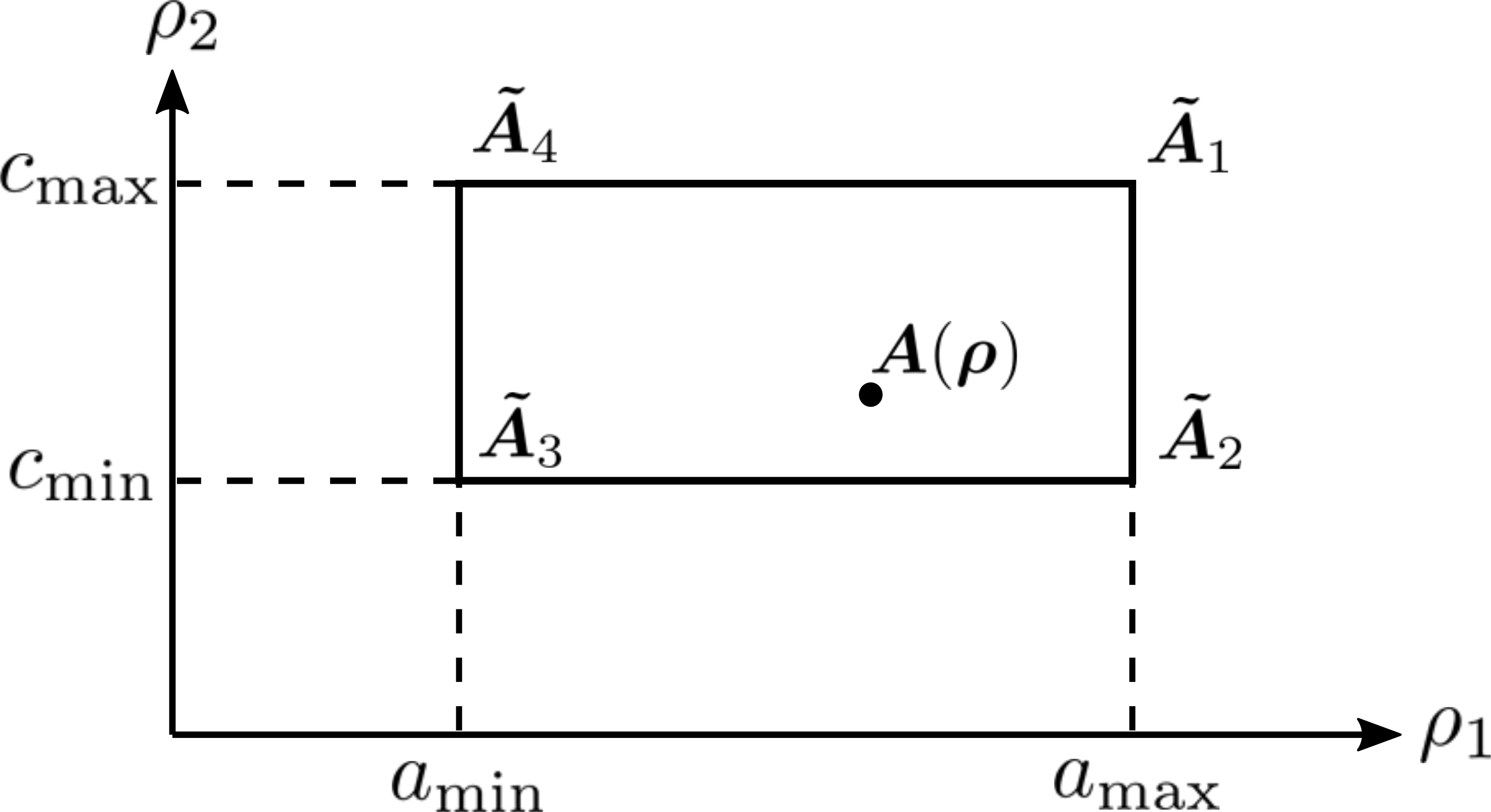
Figure 1: Polytope set represented in the parameter space.

Other matrices $\bm{\tilde{B}}_{l}$ and $\bm{\tilde{B}}_{wl}$ are formed in the same way. Note that it is important to use a sufficient number of observable functions with appropriate design to avoid ill-conditioning which leads to an extremely large size of the polytope.

III-C Construction with a Threshold Algorithm

In a practical point of view the construction of a polytope set (27) may require prohibitively high computational storage since it is necessary to evaluate $2^{N^{2}}$ vertices. Thus in order to construct a polytope set with a moderate number of vertices we apply a threshold algorithm described in Algorithm 1. We generate $2^{h}$ vertices considering not all entries but only $h$ entries whose variations within the data sets are larger than others, which are fixed to the mean values.

III-D Extended $\mathcal{H}_{2}$ Norm Characterization

With respect to the data-driven model (26), we define the controlled output $\bm{z}_{k}\in\mathbb{R}^{d}$ as follows:

$$\bm{z}_{k}=\bm{C}_{z}\bm{g}(\bm{x}_{k})+\bm{D}_{zu}\bm{u}_{k}.$$ (46)

In the proposed controller synthesis, the cost function $J_{\text{obj}}$ to be minimized is defined as:

$$J_{\text{obj}}:=\sum_{k=1}^{\infty}\bm{z}_{k}^{\mathsf{T}}\bm{z}_{k},$$ (47)

whose expected value is equivalent to the $\mathcal{H}_{2}$ norm of the model provided $\bm{w}_{k}$ is the white noise. Then the extended $\mathcal{H}_{2}$ norm characterization of the generalized plant ((26), (46)) is described as follows[19].

Theorem 1

$$\hskip 19.91692pt\left\|\mathcal{H}_{wz}\right\|_{2}^{2}<\mu\ \ \Leftrightarrow\ \ \exists\bm{P},\,\bm{W},\,\bm{X},\,\bm{L}\ \text{s.t.}$$

$$\text{tr}(\bm{W})<\mu,$$ (48)

$$\bm{M}_{1}:=\left[\begin{array}[]{cc}\bm{W}&\bm{C}_{z}\bm{X}+\bm{D}_{zu}\bm{L}\\ &\bm{X}+\bm{X}^{\mathsf{T}}-\bm{P}\end{array}\right]>0,$$ (51)

$$\bm{M}_{2}:=\left[\begin{array}[]{ccc}\bm{P}&\bm{A}(\bm{\rho})\bm{X}+\bm{B}(\bm{\rho})\bm{L}&\bm{B}_{w}(\bm{\rho})\\ &\bm{X}+\bm{X}^{\mathsf{T}}-\bm{P}&\bm{0}\\ &*&\bm{I}\end{array}\right]>0,$$ (55)

where $\bm{P}$ and $\bm{W}$ are symmetric, and $\left\|\mathcal{H}_{wz}\right\|_{2}$ denotes the $\mathcal{H}_{2}$ norm from $\bm{w}_{k}$ to $\bm{z}_{k}$.

With variables satisfying this theorem, a static feedback controller of the form (24) that guarantees the stability of the closed system and satisfies $\left\|\mathcal{H}_{wz}\right\|_{2}^{2}<\mu$ can be obtained as $\bm{S}=\bm{L}\bm{X}^{-1}$ [19].

Algorithm 1 Construction of a polytope set

Matrices $\{\bm{A}_{l}\}_{l=1}^{N_{D}}$ and the threshold number $h\in\mathbb{N}$

A set $\{\bm{\tilde{A}}_{i}\}_{i=1}^{2^{h}}$ of a polytope set

$\bm{A}_{\text{max}}(i,j)\leftarrow\underset{1\leq l\leq N_{D}}{\text{max}}[\bm{A}_{l}(i,j)]$ for $\forall$ $i,j$

$\bm{A}_{\text{min}}(i,j)\leftarrow\underset{1\leq l\leq N_{D}}{\text{min}}[\bm{A}_{l}(i,j)]$ for $\forall$ $i,j$

$\bm{A}_{\text{mean}}(i,j)\leftarrow\frac{1}{N_{D}}\sum_{l=1}^{N_{D}}\bm{A}_{l}(i,j)$ for $\forall$ $i,j$

$\bm{\tilde{A}}_{1}\leftarrow\bm{A}_{\text{mean}}$

$\bm{\tilde{A}}_{2}\leftarrow\bm{A}_{\text{mean}}$

for $p=1:h$ do

      $(s,t)\leftarrow$ index of the $p$-th largest entry of $\bm{A}_{\text{max}}-\bm{A}_{\text{min}}$

     for $k=1:2^{p-1}$ do

         $\bm{\tilde{A}}_{2^{p-1}+k}\leftarrow\bm{\tilde{A}}_{k}$

         $\bm{\tilde{A}}_{k}(s,t)\leftarrow\bm{A}_{\text{max}}(s,t)$

         $\bm{\tilde{A}}_{2^{p-1}+k}(s,t)\leftarrow\bm{A}_{\text{min}}(s,t)$

     end for

end for

III-E Robust Controller Synthesis

Using the vertex matrices $\{\bm{\tilde{A}}_{i},\bm{\tilde{B}}_{i},\bm{\tilde{B}}_{wi}\}$ of the polytope set (27) and the controlled output (46), we solve the following problem to design a robust controller that accounts for the model uncertainty due to the the data-driven procedure.

Problem 1

(Proposed Controller Synthesis)  
Given vertex matrices $\{\bm{\tilde{A}}_{i},\bm{\tilde{B}}_{i},\bm{\tilde{B}}_{wi}\}_{i=1}^{2^{h}}$, $\bm{C}_{z}$, and $\bm{D}_{zu}$, solve the following problem:

$$\text{inf tr}(\bm{W}_{i})\ \text{ subject to }$$

$$\bm{M}_{1}(\bm{P},\bm{W},\bm{X},\bm{L};\ \bm{C}_{z},\bm{D}_{zu})>0,$$

$$\bm{M}_{2}(\bm{P},\bm{X},\bm{L};\ \bm{\tilde{A}}_{i},\bm{\tilde{B}}_{i},\bm{\tilde{B}}_{wi})>0,\ \ \ \text{for }i=1,\cdots,2^{h},$$

and define $J_{\text{syn}}:=\underset{1\leq i\leq 2^{h}}{\text{max}}\{\text{tr}(\bm{W}_{i})\}$ and $\bm{S}:=\bm{L}\bm{X}^{-1}$.

We also define the following problem for evaluating the bound $J(\bm{\rho})$ for the $\mathcal{H}_{2}$ norm.

Problem 2

(Evaluation of the $\mathcal{H}_{2}$ norm)  
Given system matrices $\bm{A}(\bm{\rho})$, $\bm{B}(\bm{\rho})$, $\bm{B}_{w}(\bm{\rho})$, $\bm{C}_{z}$, $\bm{D}_{zu}$, and a feedback gain $\bm{S}$, solve the following problem:

$$\text{inf tr}(\bm{W})\ \text{ subject to }$$ (56)

$$\bm{M}_{3}:=\left[\begin{array}[]{cc}\bm{W}&\left(\bm{C}_{z}+\bm{D}_{zu}\bm{S}\right)\bm{X}\\ &\bm{X}+\bm{X}^{\mathsf{T}}-\bm{P}\end{array}\right]>0,$$ (59)

$$\bm{M}_{4}:=\left[\begin{array}[]{ccc}\bm{P}&\left(\bm{A}(\bm{\rho})+\bm{B}(\bm{\rho})\bm{S}\right)\bm{X}&\bm{B}_{w}(\bm{\rho})\\ &\bm{X}+\bm{X}^{\mathsf{T}}-\bm{P}&\bm{0}\\ &*&\bm{I}\end{array}\right]>0,$$ (63)

and define $J(\bm{\rho}):=\text{tr}(\bm{W})$.

Corollary 1

If we solve Problem 2 using a feedback gain $\bm{S}$ determined by Problem 1, then $J(\bm{\rho})\leq J_{\text{syn}}$ for $\forall\bm{\rho}$.

Proof:

It is easy to prove the proposition, and the proof is omitted due to lack of space. ∎

By Corollary 1 it is confirmed that the proposed controller guarantees that for all the plants in the polytope set (27) the $\mathcal{H}_{2}$ norm is bounded by $J_{\text{syn}}$.

III-F Relation Between the Model Uncertainty and the $\mathcal{H}_{2}$ Norm

We can relate the model uncertainty of the model, which corresponds to the parameter $\bm{\rho}$, and the bound for the $\mathcal{H}_{2}$ norm as follows.

Theorem 2

Let $\bm{A}(\bm{\rho})$, $\bm{B}(\bm{\rho})$, and $\bm{B}_{w}(\bm{\rho})$ be system matrices. Consider two sets $\mathcal{O}:=\{\bm{\rho}\}$ and $\mathcal{O}^{\prime}:=\{\bm{\rho}^{\prime}\}$ of parameters, where $J_{\text{syn}}$ and $J_{\text{syn}}^{\prime}$ denote the corresponding bounds for the $\mathcal{H}_{2}$ norm determined by Problem 1, respectively. If $\mathcal{O}\subseteq\mathcal{O}^{\prime}$, then $J_{\text{syn}}\leq J_{\text{syn}}^{\prime}$.

Proof:

It is easily shown that if $\mathcal{O}\subseteq\mathcal{O}^{\prime}$,

$$\left\{\left[\bm{A}(\bm{\rho})\bm{B}(\bm{\rho})\bm{B}_{w}(\bm{\rho})\right]\right\}\subseteq\left\{\left[\bm{A}(\bm{\rho}^{\prime})\bm{B}(\bm{\rho}^{\prime})\bm{B}_{w}(\bm{\rho}^{\prime})\right]\right\},$$ (64)

for all $\bm{\rho}$ and $\bm{\rho}^{\prime}$. Let $\Sigma:=\{[\bm{\tilde{A}}_{i}\,\bm{\tilde{B}}_{i}\,\bm{\tilde{B}}_{wi}]\}$ and $\Sigma^{\prime}:=\{[\bm{\tilde{A}}_{i}^{\prime}\,\bm{\tilde{B}}_{i}^{\prime}\,\bm{\tilde{B}}_{wi}^{\prime}]\}$ be vertex matrices that correspond to $\mathcal{O}$ and $\mathcal{O}^{\prime}$, respectively. By (64) and Corollary 1 it is shown that for any $\bm{\rho}\in\mathcal{O}$,

$$J(\bm{\rho})\leq J_{\text{syn}}^{\prime},$$ (65)

where $J_{\text{syn}}^{\prime}$ denotes the bound determined by Problem 1 with the vertices $\Sigma^{\prime}$. On the other hand, by Corollary 1 there exists $\bm{\rho}_{I}\in\mathcal{O}$ s.t. $\bm{\rho}_{I}$ corresponds to one of the vertices $\Sigma$ and

$$J(\bm{\rho}_{I})=J_{\text{syn}},$$ (66)

where $J_{\text{syn}}$ denotes the bound determined by Problem 1 with the vertices $\Sigma$. Substituting $\bm{\rho}=\bm{\rho}_{I}$ into (65),

$$J_{\text{syn}}=J(\bm{\rho}_{I})\leq J_{\text{syn}}^{\prime}\ \Leftrightarrow\ J_{\text{syn}}\leq J_{\text{syn}}^{\prime}.$$ (67)

∎

Theorem 2 states that the worst case $\mathcal{H}_{2}$ norm, which corresponds to $J_{\text{syn}}$, becomes greater if the model uncertainty becomes greater. On the other hand, it is emphasized that there may be a gap between $J_{\text{syn}}$ and $J(\bm{\rho})$, i.e., the worst case $\mathcal{H}_{2}$ norm and the actual $\mathcal{H}_{2}$ norm.

IV NUMERICAL EXAMPLES

In this section we provide simulation results of the proposed controller synthesis applied to nonlinear systems. In addition to the proposed controller we design two other controllers for comparison. One is the LQR regulator designed for a single data-driven model (26), and the other is the nominal $\mathcal{H}_{2}$ feedback controller, which we design for a single data-driven model (26) by solving the following problem:

Problem 3

(Nominal Controller Synthesis)

$$\text{inf. }\ \ \text{tr}(\bm{W})\ \text{ subject to }$$

$$\bm{M}_{1}(\bm{P},\bm{W},\bm{X},\bm{L};\ \bm{C}_{z},\bm{D}_{zu})>0,$$

$$\bm{M}_{2}(\bm{P},\bm{X},\bm{L};\ \bm{A}(\bm{\rho}),\bm{B}(\bm{\rho}),\bm{B}_{w}(\bm{\rho}))>0.$$ (68)

IV-A Duffing Oscillator

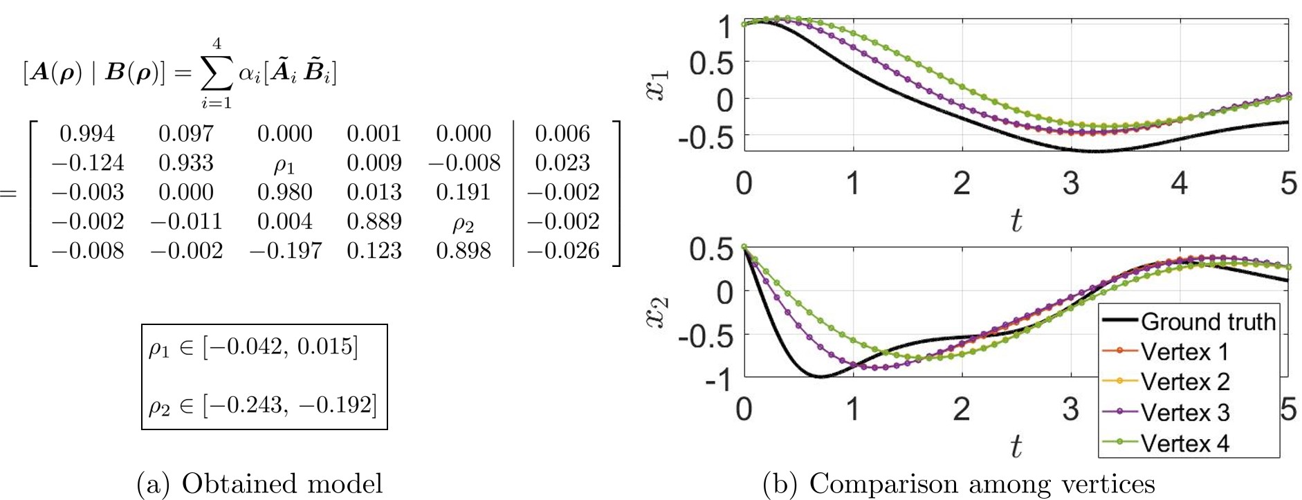
Figure 2: Data-driven model of the duffing oscillator.

As the first example we consider the forced duffing oscillator:

$$\ddot{x}+0.5\dot{x}-x+4x^{3}=u(t),$$ (69)

where $u(t)$ represents the input to the system. We assume that the trajectory of the states $\bm{x}=[x_{1}\ x_{2}]^{\mathsf{T}}$ ($x_{1}:=x,\ x_{2}:=\dot{x}$) is available as data while we have no knowledge about the governing equation. In the simulation, measurement noise $w\sim\mathcal{N}(w\mid 0,0.01)$ is added to the states. We specify the observable functions as monomials up to the second order:

$$\bm{g}(\bm{x})=[x_{1}\ \ x_{2}\ \ x_{1}^{2}\ \ x_{2}^{2}\ \ x_{1}x_{2}]^{\mathsf{T}}.$$ (70)

For the proposed controller synthesis we collect four data sets $\{D_{l}\}_{l=1}^{4}$ with the sampling interval $\Delta t=0.1$. Each data set consists of 150 pairs $(\bm{F}(\bm{x},u),\bm{x},u)$ of one-step trajectories, where $\bm{x}$ and $u$ are sampled from the uniform distribution over $[-1,1]$. In order to stabilize the states while saving the input energy we define the controlled output as $\bm{z}=\bm{C}_{z}\bm{g}(\bm{x})+\bm{D}_{zu}u=[10x_{1}\ x_{2}\ u]^{\mathsf{T}}$, where

$$\bm{C}_{z}=\left[\begin{array}[]{c}\begin{array}[]{cc}\begin{array}[]{cc}10&0\\ 0&1\end{array}&\bm{0}_{2,3}\end{array}\\ \bm{0}_{1,5}\end{array}\right],\bm{D}_{zu}=\left[\begin{array}[]{c}0\\ 0\\ 1\end{array}\right].$$ (79)

Figure 2 shows the data-driven model obtained by the proposed method and the comparison of the prediction errors among the vertices of the polytope. Note that we ignored the dependence of $\bm{\rho}$ on $\bm{B}(\bm{\rho})$ since all the variations of $\bm{B}(\bm{\rho})$ were negligibly small, and we set the threshold number $h=2$ for $\bm{A}(\bm{\rho})$.

The LQR regulator and the nominal $\mathcal{H}_{2}$ controller are designed with the single data set $D_{1}$. We select the weight matrices for the LQR regulator so that the cost function:

$$J_{LQR}=\sum_{k=1}^{\infty}\left(\bm{g}(\bm{x}_{k})^{\mathsf{T}}\bm{Q}\bm{g}(\bm{x}_{k})+\bm{u}_{k}^{\mathsf{T}}\bm{R}\bm{u}_{k}\right),$$ (80)

is equivalent to the $\mathcal{H}_{2}$ norm, i.e., we set

$$\bm{Q}=\left[\begin{array}[]{c}\begin{array}[]{cc}\begin{array}[]{cc}100&0\\ 0&1\end{array}&\bm{0}_{2,3}\end{array}\\ \bm{0}_{1,5}\end{array}\right],\ \ R=1.$$ (86)

The simulation result is shown in Fig. 3. It is observed that the proposed robust $\mathcal{H}_{2}$ controller effectively attenuates the peak of $x_{1}$ compared to the LQR and the nominal $\mathcal{H}_{2}$ controllers. As a result the $l_{2}$ norm of the proposed controller is smaller than other two controllers (Fig. 3 (d)). This result suggests that the proposed controller successfully dealt with the model uncertainty caused by the data-driven modeling procedure described in Section II, while other two controllers lower the performance in the condition 2 due to this model uncertainty.

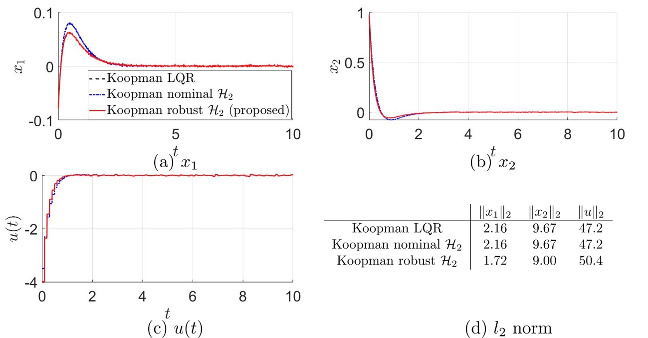
Figure 3: Result of the duffing oscillator with the initial condition: $(x_{1}(0),x_{2}(0))=(-0.08,0.97)$.

IV-B Shallow-Water Waves Control

As another example we investigate the controller performance with the Korteweg-de Vries (KdV) equation, which models the shallow-water waves:

$$\partial_{t}y(t,x)+y(t,x)\partial_{x}y(t,x)+\partial_{x}^{3}y(t,x)=u(t,x).$$ (87)

In this example the input $\bm{u}_{k}=[u_{1,k}u_{2,k}u_{3,k}]^{\mathsf{T}}$ has a structure s.t. $u(t,x)=\sum_{i=1}^{3}u_{i,k}\left\{U(t,t)-U(t,\Delta t)\right\}v_{i}(x)$, where $v_{i}(x)=e^{25\left(x-c_{i}\right)^{2}}$, $c_{1}=-\frac{\pi}{2}$, $c_{2}=0$ $c_{3}=\frac{\pi}{2}$, and $U(t,a)$ denotes the step function.

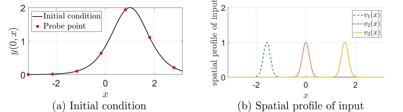
Figure 4: Initial condition and the spatial profile of input.

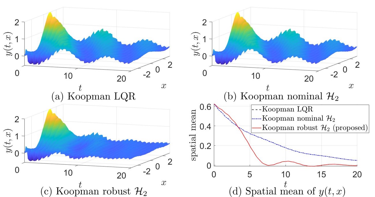
Figure 5: Result of the KdV equation.

In the simulation, the equation is discretized by the split-stepping method, which generates the state space of 128 dimensions with the time discretization of 0.01 seconds. With the sampling interval $\Delta t=0.01$ we measure the water surface $y(t,x)$ at seven probe points that are shown in Fig. 4 (a), and use them as observable functions, which are referred to as $\bm{x}_{k}$. We collect four data sets, each of which consists of 100 trajectories with a length of 200 steps, where the initial conditions are specified by random convex combinations of three spatial profiles: $e^{-(x-\pi/2)^{2}}$, $-\sin(x/2)^{2}$, and $e^{-(x+\pi/2)^{2}}$. The controlled output is set as $\bm{z}_{k}=\bm{C}_{z}\bm{g}(\bm{x}_{k})+\bm{D}_{zu}\bm{u}_{k}=[\bm{x}_{k}^{\mathsf{T}}\ \bm{u}_{k}^{\mathsf{T}}]^{\mathsf{T}}$, where

$$\bm{C}_{z}=[\bm{I}_{7}\ \bm{0}_{7,3}]^{\mathsf{T}},\ \ \bm{D}_{zu}=[\bm{0}_{3,7}\ \bm{I}_{3}]^{\mathsf{T}}.$$ (88)

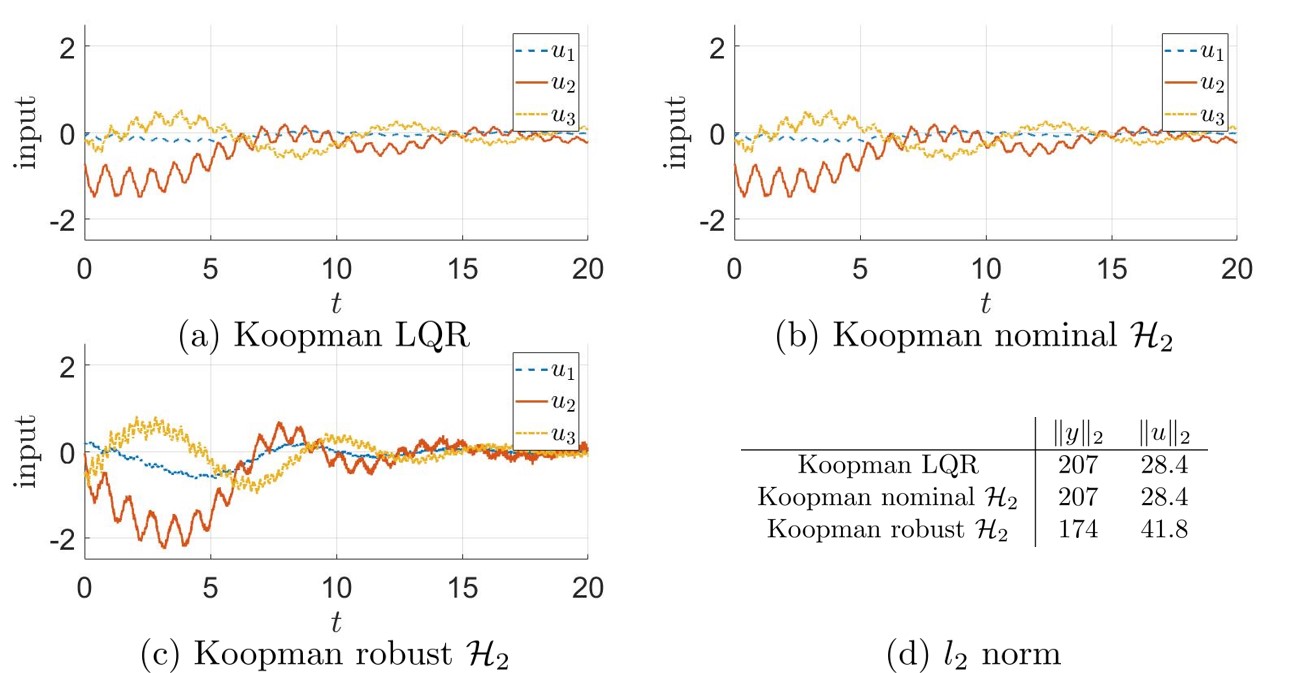
Figure 6: Input obtained by the controllers.

We set the threshold number $h=2$ for $\bm{A}(\bm{\rho})$, and ignored the dependence of $\bm{\rho}$ on $\bm{B}(\bm{\rho})$ since the variations of entries were negligibly small. The weight matrices for the LQR controller are defined as $\bm{Q}=\bm{I}_{7},\ \bm{R}=\bm{I}_{3},$ so that the cost function $J_{LQR}$ is equivalent to the $\mathcal{H}_{2}$ norm.

The result is shown Figs. 5 and 6. It is shown that the proposed controller quickly stabilized the states (Fig. 5 (c)) while other two controllers had difficulty regulating the system (Fig. 5 (a),(b)).

V CONCLUSIONS

This paper presented a data-driven control synthesis that combines the data-driven Koopman operator theory and the $\mathcal{H}_{2}$ characterization of linear systems. In order to deal with the model uncertainty due to the nature of the data-driven modeling, the proposed method models the system as a polytope set, which is then utilized to design a robust feedback controller on the basis of the $\mathcal{H}_{2}$ norm characterization. Future directions of research include the introduction of statistical properties to the proposed data-driven model.

References

- [1] M. Budišić, R. Mohr, and I. Mezić, “Applied Koopmanism,” Chaos: An Interdisciplinary Journal of Nonlinear Science, vol. 22, no. 4, p. 047510, 2012.
- [2] C. Rowley, I. Mezić, S. Bagheri, P. Schlatter, and D. S. Henningson, “Spectral analysis of nonlinear flows,” Journal of Fluid Mechanics, vol. 641, pp. 115–127, 2009.
- [3] P. Schmid, “Dynamic mode decomposition of numerical and experimental data,” Journal of Fluid Mechanics, vol. 656, pp. 5–28, 2010.
- [4] J. Tu, C. Rowley, D. Luchtenburg, S. Brunton, and N. Kutz, “On dynamic mode decomposition: Theory and applications,” Journal of Computational Dynamics, vol. 1, no. 2, pp. 391–421, 2014.
- [5] M. Williams, I. Kevrekidis, and C. Rowley, “A data driven approximation of the Koopman operator: Extending dynamic mode decomposition,” Journal of Nonlinear Science, vol. 25, no. 6, pp. 1307–1346, 2015.
- [6] M. Williams, C. Rowley, and I. Kevrekidis, “A kernel-based method for data-driven Koopman spectral analysis,” Journal of Computational Dynamics, vol. 2, no. 2, pp. 247–265, 2015.
- [7] E. Yeung, S. Kundu, and N. Hodas, “Learning deep neural network representations for Koopman operators of nonlinear dynamical systems,” Proceedings of the 2019 American Control Conference (ACC), pp. 4832–4839, 2019.
- [8] Q. Li, F. Dietrich, E. M. Bollt, and I. G. Kevrekidis, “Extended dynamic mode decomposition with dictionary learning: A data-driven adaptive spectral decomposition of the Koopman operator,” Chaos: An Interdisciplinary Journal of Nonlinear Science, vol. 27, no. 10, p. 103111, 2017.
- [9] N. Takeishi, Y. Kawahara, and T. Yairi, “Learning Koopman invariant subspaces for dynamic mode decomposition,” Advances in Neural Information Processing Systems, vol. 30, 12 2017.
- [10] J. L. Proctor, S. L. Brunton, and J. N. Kutz, “Dynamic mode decomposition with control,” SIAM Journal on Applied Dynamical Systems, vol. 15, no. 1, pp. 142–161, 2016.
- [11] J. L. Proctor, S. L. Brunton, and J. N. Kutz, “Generalizing koopman theory to allow for inputs and control,” SIAM Journal on Applied Dynamical Systems, vol. 17, no. 1, pp. 909–930, 2018.
- [12] M. O. Williams, M. S. Hemati, S. T. Dawson, I. G. Kevrekidis, and C. W. Rowley, “Extending data-driven koopman analysis to actuated systems,” IFAC-PapersOnLine, vol. 49, no. 18, pp. 704–709, 2016.
- [13] S. L. Brunton, B. W. Brunton, J. L. Proctor, and J. N. Kutz, “Koopman invariant subspaces and finite linear representations of nonlinear dynamical systems for control,” PLOS ONE, vol. 11, no. 2, pp. 1–19, 2016.
- [14] M. Korda and I. Mezić, “Linear predictors for nonlinear dynamical systems: Koopman operator meets model predictive control,” Automatica, vol. 93, pp. 149–160, 2018.
- [15] H. Arbabi, M. Korda, and I. Mezić, “A data-driven Koopman model predictive control framework for nonlinear partial differential equations,” Proceedings of the 2018 IEEE Conference on Decision and Control (CDC), pp. 6409–6414, 2018.
- [16] S. Peitz and S. Klus, “Koopman operator-based model reduction for switched-system control of PDEs,” Automatica, vol. 106, pp. 184–191, 2019.
- [17] S. Peitz, S. E. Otto, and C. W. Rowley, “Data-driven model predictive control using interpolated Koopman generators,” arXiv e-prints, p. arXiv:2003.07094, 2020.
- [18] E. Kaiser, J. N. Kutz, and S. L. Brunton, “Data-driven discovery of Koopman eigenfunctions for control,” arXiv e-prints, p. arXiv:1707.01146, 2017.
- [19] M. C. D. Oliveira, J. C. Geromel, and J. Bernussou, “Extended and norm characterizations and controller parametrizations for discrete-time systems,” International Journal of Control, vol. 75, no. 9, pp. 666–679, 2002.
- [20] D. J. Leith and W. E. Leithead, “Survey of gain-schedulinganalysis and design,” International Journal of Control, vol. 73, no. 11, pp. 1001–1025, 2000.
- [21] M. O. Williams, M. S. Hemati, S. T. Dawson, I. G. Kevrekidis, and C. W. Rowley, “Extending data-driven Koopman analysis to actuated systems,” IFAC-PapersOnLine, vol. 49, no. 18, pp. 704–709, 2016.
- [22] A. Surana, “Koopman operator based observer synthesis for control-affine nonlinear systems,” Proceedings of the 2016 IEEE 55th Conference on Decision and Control (CDC), pp. 6492–6499, 2016.
- [23] A. Surana and A. Banaszuk, “Linear observer synthesis for nonlinear systems using Koopman operator framework,” IFAC-PapersOnLine, vol. 49, no. 18, pp. 716–723, 2016.