Sliding on Manifolds:
Geometric Attitude Control with Quaternions

Abstract

This work proposes a quaternion-based sliding variable that describes exponentially convergent error dynamics for any forward complete desired attitude trajectory. The proposed sliding variable directly operates on the non-Euclidean space formed by quaternions and explicitly handles the double covering property to enable global attitude tracking when used in feedback. In-depth analysis of the sliding variable is provided and compared to others in the literature. Several feedback controllers including nonlinear PD, robust, and adaptive sliding control are then derived. Simulation results of a rigid body with uncertain dynamics demonstrate the effectiveness and superiority of the approach.

I INTRODUCTION

Attitude control is a fundamental problem in robotics and aerospace that has a rich history of research. Several controllers have been proposed that vary in complexity, robustness, and tracking performance. However, many lack strong performance guarantees in diverse flight conditions – a facet that is becoming more critical as aerial and space robots find more real-world uses. Orientation dynamics evolve in a non-Euclidean space which poses challenges for synthesizing attitude controllers since all analysis must be done on the appropriate state space manifold. One natural manifold is that formed by the special orthogonal group $\mathrm{SO(3)}$ whose elements are all the orthogonal matrices with determinant 1. Several $\mathrm{SO(3)}$ controllers have been proposed in the literature, most notably [1, 2, 3, 4], but, as shown in [5], control on $\mathrm{SO(3)}$ can at best achieve almost global stability, i.e., only trajectories in an open set converge to an equilibrium. Further, the complexity of working in $\mathrm{SO(3)}$ can make performance and robustness analysis difficult. This work will show that global closed-loop stability is possible by carefully defining quaternion-based feedback terms that capture the underling topology of their non-Euclidean state space.

An effective method to derive nonlinear controllers is through the use of so-called sliding variables. Sliding variables often simplify closed-loop stability and tracking analysis by forming a hierarchy of simple reduced order systems [6]. Once a sliding variable is chosen, several robust and adaptive nonlinear controllers can be immediately employed (see [6]). However, defining a sliding variable can be difficult when a state space is non-Euclidean. This is especially true for $\mathrm{SO(3)}$ as the error dynamics of rotation matrices are difficult to analyze and stability is limited to at best almost global. The aforementioned challenges can be circumvented by instead using quaternions, which live on the three-sphere $\mathbb{S}^{3}$, to represent orientations. Several works have synthesized attitude controllers using quaternions [7, 8, 9, 10, 11], and some have proposed quaternion-based sliding variables [12, 13, 14, 15, 16]. However, works that use sliding variables either 1) treat quaternions as if they evolve in Euclidean space and ignore the topology of $\mathbb{S}^{3}$ or 2) do not address the double covering property where the so-called unwinding phenomenon [8] can lead to longer-than-necessary attitude maneuvers.

(a) Proposed method.

(b) Method from [12].

(c) Method from [14].

Figure 1: Visualization of a rigid body (RGB axes) executing an orientation pointing maneuver during which the orientation quaternion flips sign. Vertical height corresponds to the maneuver duration. The proposed method efficiently executes the pointing maneuver by directly operating on the non-Euclidean space formed by quaternions and explicitly taking into account the double covering property of quaternions.

The main contribution of this work is a quaternion-based sliding variable that represents exponentially convergent error dynamics. Exponential convergence is achieved despite explicitly capturing the geometry of the $\mathbb{S}^{3}$ manifold. The unwinding behavior is eliminated by introducing a benign discontinuity in the sliding variable that maintains control input continuity when used in feedback. Additionally, the discontinuity results in global convergence when the sliding variable is used in feedback. When compared to other methods the proposed approach has faster convergence without unwinding and is easier to analyze. Moreover, the global stability results are much stronger than those obtainable in $\mathrm{SO(3)}$. Three controllers with strong performance guarantees (nonlinear PD, robust, and adaptive sliding control) are derived using the proposed sliding variable. The developed method stems from previous work on provably-safe UAV collision avoidance [17] where high-performance attitude control was necessary for establishing safety guarantees despite high model uncertainty. This work opens avenues for research in designing trajectories that explicitly consider how a maneuver can exacerbate or reduce the effects of model uncertainty. Simulation results confirm the predicted performance and demonstrate the benefits of the approach.

II BACKGROUND & PROBLEM FORMULATION

A unit quaternion $q$ is a four vector that lies on the three-sphere $\mathbb{S}^{3}$ and consists of a real and vector part, i.e., $q=(\,q^{\circ},\vec{q}\,)$. The set of unit quaternions form a Lie group under the multiplication operator $\otimes$, where given two quaternions $p$ and $q$ the quaternion product is

$$p\otimes q=\left[\begin{array}[]{c}p^{\circ}q^{\circ}-\vec{p}^{\top}\vec{q}\\ p^{\circ}\vec{q}+q^{\circ}\vec{p}+p\times q\end{array}\right].$$

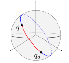
The inverse of quaternion $q$ is the conjugate quaternion $q^{*}:=(\,q^{\circ},-\vec{q}\,)$ which satisfies $q\otimes q^{*}=q^{*}\otimes q=(1,0,0,0)$. In the context of mechanics, quaternions are particularly useful for representing orientation. A rotation about a vector $\hat{n}$ through angle $\phi$ can be compactly expressed as $q=(\mathrm{cos}(\nicefrac{{\phi}}{{2}}),\mathrm{sin}(\nicefrac{{\phi}}{{2}})\hat{n})$. Quaternions double cover the special orthogonal group $\mathrm{SO}(3)$ so $q$ and $-q$ represent the same orientation. There are then two potential “shortest paths” that connect any two quaternions (see Fig. 2). The so-called unwinding phenomenon occurs when the longer path (blue curve in Fig. 2) is selected resulting in a longer-than-necessary maneuver. From a practical and theoretical point of view, any quaternion-based algorithm must capture the geometric properties of the Lie group they form. Put simply, quaternions must not be treated as vectors in $\mathbb{R}^{4}$.

The quaternion attitude dynamics can be expressed as

$$\dot{q} =\frac{1}{2}q\otimes\left[\begin{array}[]{c}0\\ \omega\end{array}\right]$$ (1)

$$J\dot{\omega} =-\omega\times J\omega+f(q,\omega)+M_{b}+d,$$

with $q$ and $\otimes$ are defined as before, angular velocity $\omega\in\mathbb{R}^{3}$, symmetric positive-definite inertia tensor $J\in\mathscr{S}^{3}_{+}$, control input $M_{b}\in\mathbb{R}^{3}$, unknown dynamics $f:\mathbb{S}^{3}\times\mathbb{R}^{3}\rightarrow\mathbb{R}^{3}$, and unknown disturbance $d\in\mathbb{R}^{3}$.

The goal of this work is to define a sliding variable that represents exponentially convergent error dynamics while capturing the geometry of the Lie group formed by quaternions. By directly considering the topology of $\mathbb{S}^{3}$ the proposed sliding variable should result in faster tracking error convergence than if they were treated as vectors in Euclidean space. Additionally, global convergence results, rather than almost global, should be achieved if the sliding variable is designed carefully.

III SLIDING VARIABLES ON MANIFOLDS

III-A Overview

Stability analysis and tracking performance evaluation can be simplified through the use of so-called sliding variables. If an appropriate sliding variable can be defined then all analysis can be performed on a simpler reduced-ordered system. For instance, if a hierarchical system is formed by selecting the sliding variable $s$ to describe the desired tracking error dynamics, then the trajectory tracking problem reduces to finding a feedback policy that makes the manifold $\mathcal{S}:=\{(\vec{q}_{e},\omega_{e}):s(\vec{q}_{e},\omega_{e})=0\}$ invariant. In most cases defining a sliding variable is trivial since many systems operate in $\mathbb{R}^{n}$. For systems that lie on a manifold other than $\mathbb{R}^{n}$, such as $\mathbb{S}^{3}$ or $\mathrm{SO(3)}$, it can be difficult to construct a sliding variable with simple exponentially convergent error dynamics. This section will first present a quaternion-based sliding variable that captures the geometry of $\mathbb{S}^{3}$ with tracking error dynamics that are globally exponentially convergent. The proposed quaternion-based sliding variable is then compared to a few common $\mathbb{S}^{3}\times\mathbb{R}^{3}$ and $\mathrm{SO(3)}\times\mathbb{R}^{3}$ alternatives.

III-B Sliding Variables in $\mathbb{S}^{3}\times\mathbb{R}^{3}$

Consider the error quaternion $q_{e}:=q_{d}^{*}\otimes q$ where $q_{d}^{*}$ is the conjugate of the desired quaternion and $q$ is the current quaternion. The error quaternion has dynamics

$$\dot{q}_{e}=\frac{1}{2}q_{e}\otimes\left[\begin{array}[]{c}0\\ \omega_{e}\end{array}\right]=\left[\begin{array}[]{c}-\vec{q}_{e}^{\top}\omega_{e}\\ q_{e}^{\circ}\omega_{e}+\vec{q}_{e}\times\omega_{e}\end{array}\right].$$ (2)

Let the sliding variable $s$ be defined as

$$s=\omega_{e}+\lambda\mathrm{sgn}_{+}\left(q_{e}^{\circ}\right)\vec{q}_{e},$$ (3)

with $\omega_{e}:=\omega-\omega_{d}$, $\lambda>0$, and

$$\mathrm{sgn}_{+}(\cdot):=\begin{cases}1&\mathrm{if}~{}\cdot\geq 0\\ -1&\mathrm{if}~{}\cdot<0.\end{cases}$$ (4)

Note that all operations in Equation 3 are element-wise. The function $\mathrm{sgn}_{+}$ in Equation 4 is different than its standard definition but is necessary for establishing global exponential convergence. Proposition 1 shows that if the manifold $\mathcal{S}$ is made invariant via feedback then the the error quaternion $q_{e}$ converges to the identity quaternion exponentially.

Figure 2: Illustration of the double covering property of quaternions in $\mathbb{S}^{2}$. Two valid paths (red and blue) connect the actual $q$ and desired quaternion $q_{d}$. The so-called unwinding phenomenon occurs when a longer path (blue) is taken to reach the desired quaternion $q_{d}$.

Proposition 1.

Assume that the manifold $\mathcal{S}=\{(\vec{q}_{e},\omega_{e}):s(\vec{q}_{e},\omega_{e})=0\}$ is invariant. Then, for any trajectory initialized on $\mathcal{S}$, the quaternion error $q_{e}$ converges to the identity quaternion exponentially.

Proof.

First assume the manifold $\mathcal{S}$ is invariant, i.e., $s=0$ for all $t\geq t_{0}$. Then, from Equation 3,

$$\omega_{e}+\lambda\mathrm{sgn}_{+}\left(q_{e}^{\circ}\right)\vec{q}_{e}=0.$$ (5)

Now consider the candidate Lyapunov function $V=\|\vec{q}_{e}\|^{2}$. Differentiating along the quaternion error dynamics Equation 2,

$$\dot{V}=2\vec{q}_{e}^{\top}\dot{\vec{q}}_{e}=2\vec{q}_{e}^{\top}\left[-q_{e}^{\circ}\omega_{e}+\vec{q}_{e}\times\omega_{e}\right]=-2q_{e}^{\circ}\vec{q}_{e}^{\top}\omega_{e},$$ (6)

where the third equality is obtained by noting the cross product between $\vec{q}_{e}$ and $\omega_{e}$ produces a vector perpendicular to $\vec{q}_{e}$. Since $s=0$ by assumption, Equation 5 can be substituted into Equation 6 resulting in

$$\dot{V}=\frac{d}{dt}\|\vec{q}_{e}\|^{2}=-2\lambda|q_{e}^{\circ}|\|\vec{q}_{e}\|^{2},$$ (7)

which shows $\vec{q}_{e}$ converges exponentially to zero with rate $\lambda|q_{e}^{\circ}|$. When $q_{e}^{\circ}=0$, i.e., if $\|\vec{q}_{e}\|^{2}=1$, from Equation 2 $\dot{q}_{e}^{\circ}=-\vec{q}_{e}^{\top}\omega_{e}=\lambda\mathrm{sgn}_{+}(q_{e}^{\circ})\|\vec{q}_{e}\|^{2}$ where Equation 5 is again utilized. With the definition of $\mathrm{sgn}_{+}$ in Equation 4, then $\dot{q}_{e}^{\circ}>0$ when $q_{e}^{\circ}=0$ which guarantees that $\frac{d}{dt}\|\vec{q}_{e}\|^{2}=0$ for all $t\geq t_{0}$ only when $\|\vec{q}_{e}\|=0$. Hence, $\vec{q}_{e}$ converges to zero exponentially. Furthermore, the error quaternion $q_{e}$ globally converges to the identity quaternion exponentially. ∎

Proposition 1 shows that global exponential convergence to the identity quaternion occurs with Equation 3 when $s=0$ indefinitely. This is a much stronger result than what is obtainable in $\mathrm{SO(3)}$. Additionally, since the convergence is exponential, if $s\neq 0$ but tends to zero then the error quaternion will tend to the identity quaternion. This property is key to show convergence with adaptive controllers that utilize sliding variables, and will be discussed further in Section IV-D.

The importance of capturing the topology of $\mathbb{S}^{3}$ in Equation 3 can be understood by analyzing the convergence of the sliding variable proposed in [12]; the key difference being how the quaternion error is defined. First let $[\cdot]_{\times}$ be the operator that maps a vector to a skew symmetric matrix, i.e., $[\cdot]_{\times}:\mathbb{R}^{3}\rightarrow\mathfrak{so}(3)$ where $\mathfrak{so}(3)$ is the Lie Algebra of $\mathrm{SO(3)}$. Now let $T(q):=q^{\circ}I+[\,\vec{q}\,]_{\times}$ where $T(q)$ is invertible except when $q^{\circ}=0$. Define a different sliding variable as

$$s^{\prime}=\tilde{\omega}+\lambda\tilde{q},$$ (8)

where $\tilde{\omega}:=\omega-2T(q)^{-1}\dot{\vec{q}}_{d}$ and $\tilde{q}:=\vec{q}-\vec{q}_{d}$. It can be shown that when $s^{\prime}=0$ then

$$\dot{\tilde{q}}=-\frac{1}{2}\lambda T(q)\tilde{q}.$$ (9)

For the Lyapunov-like function $V=\|\tilde{q}\|^{2}$, using Equation 9 leads to

$$\dot{V}=\frac{d}{dt}\|\tilde{q}\|^{2}\leq-\lambda q^{\circ}\|\tilde{q}\|^{2},$$ (10)

which shows $\tilde{q}\rightarrow 0$ exponentially for $q^{\circ}>0$. While Equation 10 is similar to Equation 7, the convergence behavior is quite different: it takes longer to reach the desired quaternion $q_{d}$ using the sliding variable Equation 8 than with Equation 3. From a differential geometry perspective, this is not surprising since the shortest path between two points in $\mathbb{S}^{3}$ is known to be a great arc on $\mathbb{S}^{3}$. By treating quaternions as vectors in $\mathbb{R}^{4}$, the vector difference in Equation 8 inherently leads to slower convergence since $\tilde{q}\not\in\mathbb{S}^{3}$. By properly defining the quaternion error $q_{e}$ in Equation 3, the sliding variable $s$ is guaranteed to remain on the manifold $\mathbb{S}^{3}\times\mathbb{R}^{3}$ resulting in faster convergence. Hence, the geometric properties of the state space manifold must be captured when designing sliding variables if the desired performance is to be achieved.

Another noteworthy comment on Equation 3 is the definition of $\mathrm{sgn}_{+}$ in Equation 4. If the standard function $\mathrm{sgn}$ were to be used in Equation 3 in place of Equation 4 then the sliding surface $\mathcal{S}$ would have two stable equilibria, mainly $\left(q_{e}^{\circ},\|\vec{q}_{e}\|\right)=(\pm 1,0)$ and $\left(q_{e}^{\circ},\|\vec{q}_{e}\|\right)=(0,\pm 1)$. With the choice of Equation 4, the second equilibrium is made unstable and $q_{e}$ exponential convergences to $(\pm 1,0)$. Moreover, since $q$ and $-q$ represent the same orientation, exponential convergence is indeed global. While the discontinuity in Equation 3 may seem disconcerting, the $\mathrm{sgn}_{+}$ function actually maintains continuity of a control input when $s$ is used in feedback. Furthermore, it ensures the controller selects the shortest path to the desired orientation $q_{d}$ subsequently avoiding the unwinding phenomenon that can be observed with other quaternion-based controllers (such as [14, 18]). This behavior can be deduced by noting if $q_{e}^{\circ}<0$ then the rotation is more the $\pi$ radians. Taking the conjugate of $q_{e}$, i.e., negating $\vec{q}_{e}$, results in a rotation less than $\pi$ radians as desired. If, for instance, $\mathrm{sgn}_{+}$ is omitted from Equation 3 then Equation 7 becomes $\dot{V}=-2\lambda q_{e}^{\circ}\|\vec{q}_{e}\|^{2}$ which is unstable for $q_{e}^{\circ}<0$ and unwinding occurs. The above points will be further confirmed with the results presented in Section V.

III-C Comparison to Sliding Variables in $\mathrm{SO(3)}\times\mathbb{R}^{3}$

The two stated advantages of using the quaternion-based sliding variable Equation 3 are 1) exponential convergence of the error quaternion and 2) the convergence result is global; both of which are straightforward to show. If a sliding variable is instead defined in $\mathrm{SO(3)}$, then neither of the previous statements are necessarily true let alone easy to prove. For one, stability analysis with rotation matrices can become fairly difficult. For another, at best only almost global convergence results are possible. This section will briefly discuss a recently proposed $\mathrm{SO(3)}$ sliding variable [18], which, despite its simple structure, is quite difficult to analyze until it is represented with quaternions.

First let $R\in\mathrm{SO(3)}$ which has kinematics $\dot{R}=R[\omega]_{\times}$. If $R_{d}$ is the desired rotation matrix then the error rotation matrix is $R_{e}=R_{d}^{\top}R$ with kinematics

$$\dot{R}_{e}=\left(R_{d}[\omega_{d}]_{\times}\right)^{\top}R+R_{d}^{\top}R[\omega]_{\times}=R_{e}[\breve{\omega}_{e}]_{\times},$$ (11)

where $\breve{\omega}_{e}:=\omega-R_{e}^{\top}\omega_{d}$. Let $\mathcal{P}(A):=\frac{1}{2}\left(A-A^{\top}\right)$ be the skew symmetric part of matrix $A$. Additionally, let $(\cdot)^{\vee}$ denote the inverse map of $[\cdot]_{\times}$. A candidate $\mathrm{SO(3)}$ sliding variable is then

$$s_{R}=\breve{\omega}_{e}+\lambda\left(\mathcal{P}(R_{e})\right)^{\vee}.$$ (12)

For the candidate Lyapunov function $V_{R}=\mathrm{trace}\left(3I-R_{e}\right)$ and under the condition $s_{R}=0$ indefinitely, one can show

$$\dot{V}_{R}=-\frac{\lambda}{2}\|\left(\mathcal{P}(R_{e})\right)^{\vee}\|^{2}\leq 0,$$ (13)

which indicates almost global asymptotic convergence of $R_{e}$ to $I$. This is a much weaker result than Proposition 1 and would preclude Equation 12 from being used for feedback in adaptive control. However, if one were to convert Equation 13 to a quaternion representation, then almost global exponential stability can be established in a straightforward manner [19]. Of course other $\mathrm{SO(3)}$ sliding variables can be defined, e.g., [20], but are not as simple in structure to Equation 12 and are just as complicated – if not more so – to analyze. This not only demonstrates the complexity of defining sliding variables in $\mathrm{SO(3)}$ but also how quaternions can simplify analysis and lead to stronger results.

IV CONTROL WITH $\mathbb{S}^{3}\times\mathbb{R}^{3}$ SLIDING VARIABLES

IV-A Overview

This section shows how the quaternion-based sliding variable presented in Section III can be used by several feedback controllers, including robust and adaptive controllers. The following assumptions are made regarding system Equation 1.

Assumption 1.

The disturbance $d$ belongs to a known closed convex set, i.e., $d\in\mathcal{D}:=\{d:|d|\leq D\}$.

Remark 1.

The operation $|\cdot|$ is element-wise so $D\in\mathbb{R}^{3}_{\geq 0}$.

Assumption 2.

The uncertainty in dynamics $f$ is additive and upper bounded, i.e., $f(q,\omega)=\hat{f}(q,\omega)+\tilde{f}(q,\omega)$ where $\hat{f}$ is the nominal dynamics and $|\tilde{f}(q,\omega)|\leq\mathcal{F}(q,\omega)$ is the uncertain dynamics.

Remark 2.

The operation $|\cdot|$ is element-wise so $\mathcal{F}:\mathbb{S}^{3}\times\mathbb{R}^{3}\rightarrow\mathbb{R}^{3}_{\geq 0}$.

Assumption 3.

The uncertainty in inertia tensor is additive and bounded, i.e., $J=\hat{J}+\tilde{J}$ where $\hat{J}$ is the nominal inertia tensor and $|\tilde{J}_{i,j}|\leq\mathcal{J}_{i,j}$ is the uncertain part.

IV-B Nonlinear PD Sliding Control with Feedforward

Before considering the more general case of uncertain dynamics, it is instructive to analyze the scenario where only an unknown but bounded disturbance acts on Equation 1. Section IV-D will address the scenario where the model is only partially known. Theorem 1 shows that with Equation 3 and under Assumption 1 a nonlinear PD controller with feedfoward results in global exponential closed-loop stability for forward complete desired trajectories.

Theorem 1.

Consider system Equation 1 with known dynamics $f$ and inertia tensor $J$. For a bounded disturbance $d$, the tracking error convergences exponentially to a region near the identity quaternion with the control law

$$M_{b}=J\dot{\omega}_{d}+\omega\times J\omega+f(q,\omega)-\lambda J\mathrm{sgn}_{+}(q_{e}^{\circ})\dot{\vec{q}}_{e}-Ks$$ (14)

where $s$ is the sliding variable Equation 3, $K=[k_{1},k_{2},k_{3}]^{\top}$, and $Ks$ is a vector with elements $k_{i}s_{i}$ for $i=1,2,3$.

Proof.

Consider the candidate Lyapunov function $V=s^{\top}Js$ where $s=\omega_{e}+\lambda\mathrm{sgn}_{+}(q_{e}^{\circ})\vec{q}_{e}$. Differentiating along the $s$ dynamics,

$$\dot{V}= ~{}2s^{\top}J\dot{s}=2s^{\top}\left[J\dot{\omega}-J\dot{\omega}_{d}+\lambda J\mathrm{sgn}_{+}(q_{e}^{\circ})\dot{\vec{q}}_{e}\right]$$

$$= ~{}2s^{\top}\left[-\omega\times J\omega+f(q,\omega)+M_{b}+d\right.$$

$$\left.-J\dot{\omega}_{d}+\lambda J\mathrm{sgn}_{+}(q_{e}^{\circ})\dot{\vec{q}}_{e}\right]$$

Using Equation 14,

$$\dot{V}=-2\sum_{i=1}^{3}\left(k_{i}s_{i}^{2}-s_{i}d_{i}\right)$$

Since $J$ is symmetric and positive-definite matrix then $\underaccent{\bar}{\alpha}I\leq J\leq\bar{\alpha}I$ for $\underaccent{\bar}{\alpha},~{}\bar{\alpha}>0$. By Assumption 1, each $s_{i}$ satisfies

$$|s_{i}(t)|\leq\frac{1}{\sqrt{\underaccent{\bar}{\alpha}}}|s_{i}(0)|e^{-k_{i}t}+\frac{D_{i}}{k_{i}\sqrt{\underaccent{\bar}{\alpha}}}\left(1-e^{-k_{i}t}\right),$$

which shows $|s_{i}(t)|\leq\nicefrac{{D_{i}}}{{k_{i}\sqrt{\underaccent{\bar}{\alpha}}}}$ as $t\rightarrow\infty$ exponentially. Therefore, since $s$ and the error dynamics form a hierarchy, the error dynamics converge exponentially to region near the identity quaternion. ∎

Remark 3.

The $\mathrm{sgn}_{+}$ term ensures $M_{b}$ remains continuous if the error quaternion $q_{e}$ were to slip sign during a maneuver. Smooth control is therefore guaranteed because the sliding variable contains a discontinuity.

Theorem 1 showed that a nonlinear PD controller with feedforward and the sliding surface defined in Equation 3 results in global exponential closed-loop stability. The term “nonlinear PD” is appropriate due to the presence of $\dot{\vec{q}}_{e}$ in Equation 14, which, from Equation 2, is $\dot{\vec{q}}_{e}=q_{e}^{\circ}\omega_{e}+\vec{q}_{e}\times\omega_{e}$ and arises from the geometry of $\mathbb{S}^{3}$. For comparison, a commonly used quaternion-based PD controller without feedforward originally proposed in [7], later applied to aerial robots in [9], and used in [21] is of the form

$$M_{b}^{pd}=-\mathrm{sgn}(q_{e}^{\circ})K_{p}\vec{q}_{e}-K_{d}\omega,$$

where $K_{p},K_{d}>0$ and all products are element-wise. It is straightforward to show global asymptotic closed-loop stability via the LaSalle invariance principle for any $q_{d}$ and $\omega_{d}=0$. However, little can be said about the performance of the controller for arbitrary $\omega_{d}$. In applications where $\omega_{d}$ is not trivially zero, such as time-varying attitude tracking for spacecraft pointing or even UAV obstacle avoidance, a controller like the one presented in Theorem 1 is required for better closed-loop performance.

IV-C Robust Sliding Control

The controller presented in Section IV-B works well when only an unknown but bounded disturbance is present. As discussed previously, the main advantage of using sliding variables is that several robust and adaptive controllers can be immediately employed. One such controller is the well-known sliding mode controller which is able to achieve zero tracking error exponentially through high-frequency control switching. This so-called chattering behavior is synonymous with sliding mode control and makes it unusable for many applications. This section will instead present a continuous version known as the boundary layer sliding controller. Theorem 2 shows how the sliding variable defined in Equation 3 in conjunction with a robust controller gain leads to global exponential closed-loop stability despite model uncertainty.

Theorem 2.

For system Equation 1 with unknown disturbances, dynamics, and inertia tensor that satisfy Assumptions 1-3, the sliding variable $s$ from Equation 3 converges in finite time to the region $|s|\leq\Phi$ with the control law

$$M_{b}=\hat{J}\dot{\omega}_{d}+\omega\times\hat{J}\omega+\hat{f}(q,\omega)-\lambda\hat{J}\mathrm{sgn}_{+}(q_{e}^{\circ})\dot{\vec{q}}_{e}-K\mathrm{sat}\left(\nicefrac{{s}}{{\Phi}}\right),$$ (15)

where $\mathrm{sat}$ is the saturation function, $\Phi\in\mathbb{R}^{3}_{>0}$ is the boundary layer thickness, and $K\mathrm{sat}\left(\nicefrac{{s}}{{\Phi}}\right)$ is a vector of elements $k_{i}\mathrm{sat}\left(\nicefrac{{s_{i}}}{{\Phi_{i}}}\right)$. The robust gains $k_{i}$ satisfy

$$k_{i}\geq ~{}\left|\omega\times\tilde{J}\omega\right|_{i}+\left(\mathcal{J}\left|\dot{\omega}_{d}+\lambda\mathrm{sgn}\left(q_{e}^{\circ}\right)\dot{\vec{q}}_{e}\right|\right)_{i}$$ (16)

$$+\mathcal{F}_{i}+D_{i}+\eta_{i},$$

where $\eta_{i}>0$ and $(\cdot)_{i}$ denotes the $i^{th}$ element of vector $(\cdot)$. Furthermore, the error quaternion converges exponentially to a region near the identity quaternion.

Proof.

Let $s_{\Delta}:=s-\Phi~{}\mathrm{sat}\left(\nicefrac{{s}}{{\Phi}}\right)$ and consider the candidate Lyapunov function $V=s_{\Delta}^{\top}Js_{\Delta}$ where $V=0$ when $|s|=\Phi$ and $V>0$ when $|s|\geq\Phi$. Differentiating along the $s_{\Delta}$ dynamics (which are identical to the $s$ dynamics in this case),

$$\dot{V}= ~{}2s_{\Delta}^{\top}J\dot{s}_{\Delta}=2s_{\Delta}^{\top}\left[J\dot{\omega}-J\dot{\omega}_{d}+\lambda J\mathrm{sgn}_{+}(q_{e}^{\circ})\dot{\vec{q}}_{e}\right]$$

$$= ~{}2s_{\Delta}^{\top}\Big{[}-\omega\times J\omega+f(q,\omega)+M_{b}+d$$

$$-J\dot{\omega}_{d}+\lambda J\mathrm{sgn}_{+}(q_{e}^{\circ})\dot{\vec{q}}_{e}\Big{]}.$$

Using the control law Equation 15 and noting $\mathrm{sat}\left(\nicefrac{{s}}{{\Phi}}\right)=\mathrm{sgn}(s_{\Delta})$,

$$\dot{V}= ~{}2s_{\Delta}^{\top}\Big{[}-\omega\times\tilde{J}\omega+\tilde{f}(q,\omega)+d+\tilde{J}\omega_{d}$$ (17)

$$+\lambda\tilde{J}\mathrm{sgn}_{+}\left(q_{e}^{\circ}\right)\dot{\vec{q}}_{e}-K\mathrm{sgn}\left(s_{\Delta}\right)\Big{]}$$

$$= -2\sum_{i=1}^{3}k_{i}|s_{\Delta}|_{i}-2s_{\Delta}^{\top}\Big{[}-\omega\times\tilde{J}\omega+\tilde{f}(q,\omega)$$

$$+d+\tilde{J}\omega_{d}+\lambda\tilde{J}\mathrm{sgn}_{+}\left(q_{e}^{\circ}\right)\dot{\vec{q}}_{e}\Big{]}$$

$$\leq -2\sum_{i=1}^{3}|s_{\Delta}|_{i}\Big{[}k_{i}+|\omega\times\tilde{J}\omega|_{i}$$

$$+\left(\mathcal{J}\left|\dot{\omega}_{d}+\lambda\mathrm{sgn}\left(q_{e}^{\circ}\right)\dot{\vec{q}}_{e}\right|\right)_{i}+\mathcal{F}_{i}+D_{i}\Big{]}$$

$$\leq -2\sum_{i=1}^{3}\eta_{i}|s_{\Delta}|_{i},$$

where the inequality is obtained by using the robust gain $K$ from Equation 16. Equation 17 shows that $s_{\Delta}$ converges in finite time to zero and, since $s_{\Delta}=s-\Phi~{}\mathrm{sat}\left(\nicefrac{{s}}{{\Phi}}\right)$, $s$ converges in finite time to the region $|s|\leq\Phi$. Therefore, since $s$ and the error quaternion form a hierarchy, the error quaternion globally converges exponentially to a region, defined by the boundary layer thickness $\Phi$, near the identity quaternion. ∎

Remark 4.

Remark 3 also holds for controller Equation 15.

Remark 5.

The boundary layer in Theorem 2 can be made time-varying to capture the effects of state-dependent uncertainty on the tracking error [6]. A time varying-boundary layer is extremely useful in the context of motion planning and predictive control since they essentially represent a dynamic robust control invariant tube which can be used to robustly tighten safety constraints (see, e.g., [22, 23]).

Theorem 2 showed that the error quaternion globally converges exponentially to a region near the identity quaternion despite the presence of model error and external disturbances. This is made possible by making the manifold $\mathcal{S}_{\Phi}=\{(\vec{q}_{e},\omega_{e}):|s(\vec{q}_{e},\omega_{e})|\leq\Phi\}$ invariant with the robust control gain defined in Equation 16. However, the robust gain $K$ can become large for systems with high model uncertainty as it must handle all possible model and disturbance realizations. Adaptive control is one such method to reduce the robust gain $K$ and lower the control effort from feedback.

IV-D Adaptive Sliding Control

The performance of the nonlinear PD controller and the robust controller derived in Sections IV-B and IV-C can be improved by learning the unknown model parameters. The nonlinear PD controller can be extended to systems with uncertain dynamics (not handled in Theorem 1), while the robust gain $K$ in Theorem 2 can be reduced. To proceed the following standard assumption is made about Equation 1.

Assumption 4.

The dynamics in Equation 1 can be expressed as a linear combination of unknown parameters $a\in\mathbb{R}^{p}$, i.e., $J\dot{\omega}=J\dot{\omega}_{r}+Y(q,\omega,\dot{\omega}_{r})^{\top}a+M_{b}$ where $Y:\mathbb{S}^{3}\times\mathbb{R}^{3}\times\mathbb{R}^{3}\rightarrow\mathbb{R}^{p\times 3}$ and $\omega_{r}:=\omega_{d}-\lambda J{\vec{q}}_{e}$.

Adaptive control for systems like Equation 1 have been extensively studied and a number of approaches exists. However, only recently have methods been developed that impose physical consistency on parameters, e.g., the inertia tensor being positive-definite, during adaptation [24, 25]. This is possible by employing the Bregman divergence operator

$$\mathrm{d}_{\psi}(y~{}\|~{}x)=\psi(y)-\psi(x)-(y-x)^{\top}\nabla\psi(x),$$ (18)

where $\psi$ is a strictly convex, continuously differentiable function on a closed convex set. The time derivative of the Bregman divergence is

$$\dot{\mathrm{d}}_{\psi}(y~{}\|~{}x)=(x-y)^{\top}\nabla^{2}\psi(x)\dot{x},$$ (19)

which will be useful in the context of adaptive control. Physical consistency is enforced by appropriately selecting $\psi$, such as the log-det function for positive-definite matrices or the log function for bounded parameters. Another useful property of the Bregman divergence, eloquently shown in [26], is enforcing sparsity in $\hat{a}$ through appropriate selection of $\psi$. Theorem 3 shows how the controller in Equation 15 can be extended to uncertain systems by adding parameter adaptation that enforces physical consistency.

(a) Tracking error along body $x$-axis.

(b) Tracking error along body $y$-axis.

(c) Tracking error along body $z$-axis.

Figure 3: Comparison of tracking error with $q_{d}=(0.707,0,-0.707,0)$ and $q=(0,1,0,0)$ for a nonlinear PD controller with the proposed sliding variable and those in [12, 14]. The pink circle represents the initial error. The quaternion flips sign midway through maneuver. The tracking error with the proposed sliding variable (blue) converges to one of the two possible sliding manifolds (black). The controller from [12] exhibits undesirable convergence because quaternions are treated as Euclidean vector. The controller in [14] is similar to the proposed but exhibits unwinding (switches to different sliding manifold).

Theorem 3.

Consider system Equation 1 subject to Assumptions 3 an 4. The error quaternion asymptotically converges to the identity quaternion with the nonlinear PD controller

$$M_{b}=Y(q,\omega,\dot{\omega}_{r})^{\top}\hat{a}-Ks$$ (20)

and adaptation law

$$\dot{\hat{a}}=-\left(\nabla^{2}\psi(\hat{a})\right)^{-1}Y(q,\omega,\dot{\omega}_{r})s$$ (21)

where ${\omega}_{r}=\omega_{d}-\lambda\mathrm{sgn}_{+}(q_{e}^{\circ})\dot{\vec{q}}_{e}$ and $\psi$ is a continuously differentiable convex function.

Proof.

Consider the candidate Lyapunov function

$$V=s^{\top}Js+2\mathrm{d}_{\psi}\left(a~{}||~{}\hat{a}\right).$$ (22)

Differentiating along the $s$ dynamics and utilizing Eqs. 20 and 19,

$$\dot{V}= ~{}2s^{\top}\left[Y(q,\omega,\dot{\omega}_{r})^{\top}\tilde{a}-Ks\right]+2\tilde{a}^{\top}\nabla^{2}\psi(\hat{a})\dot{\hat{a}}.$$

With the adaptation law Equation 21 $\dot{V}=-2\sum_{i=1}^{3}k_{i}s_{i}^{2}\leq 0$. It is easy to verify that $\dot{s}$ is bounded under the condition that the desired angular acceleration $\dot{\omega}_{d}$ is bounded. By Barbalat’s lemma, $s$ approaches zero asymptotically. Therefore, by Proposition 1, the error quaternion $q_{e}$ also tends to the identity quaternion as desired. ∎

Remark 6.

The adaptation law Equation 21 can be immediately used with the robust sliding controller Equation 15 if adaptation is performed on a subset of unknown parameters. This is advantageous because the robust gain Equation 16 has fewer uncertain parameters to compensate for resulting in lower control effort. Proof omitted for brevity but similar to Theorem 3.

V RESULTS

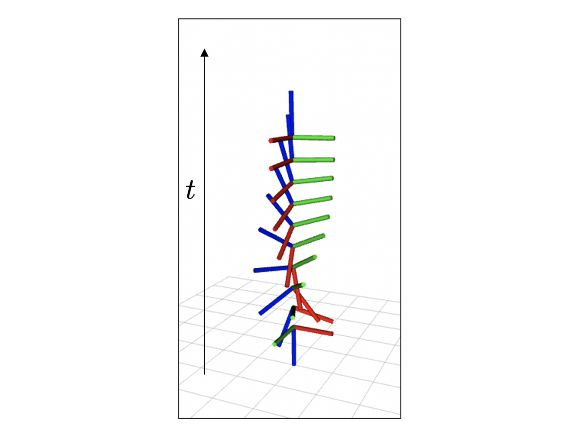
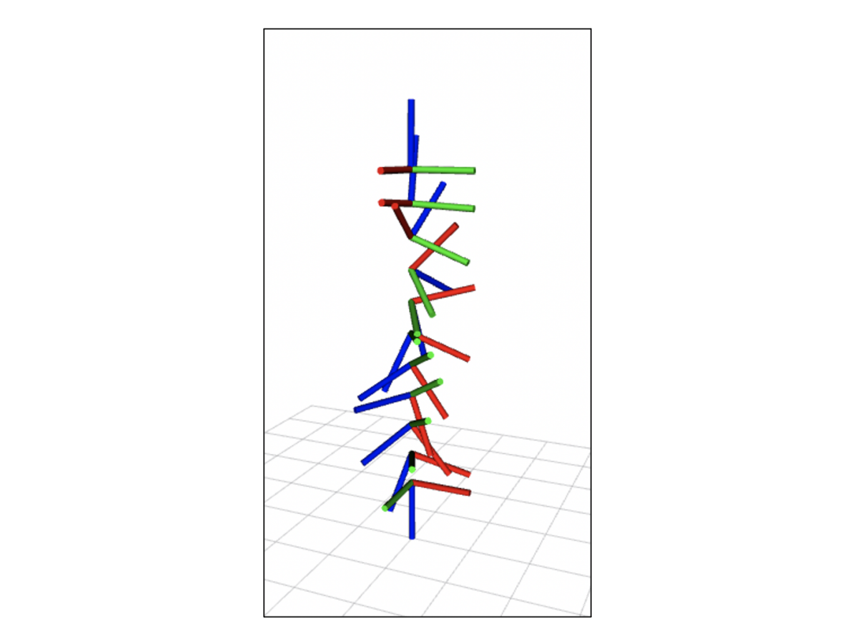
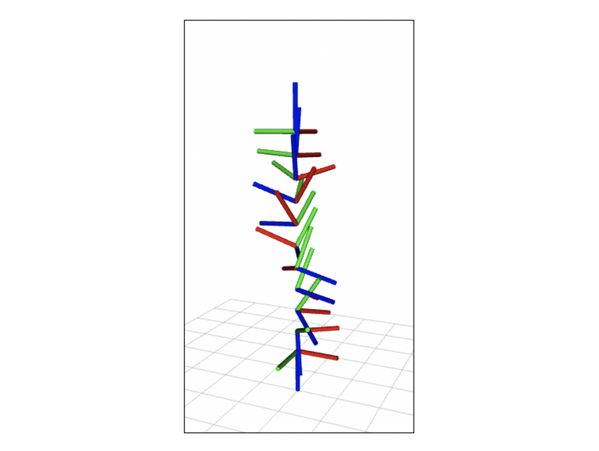
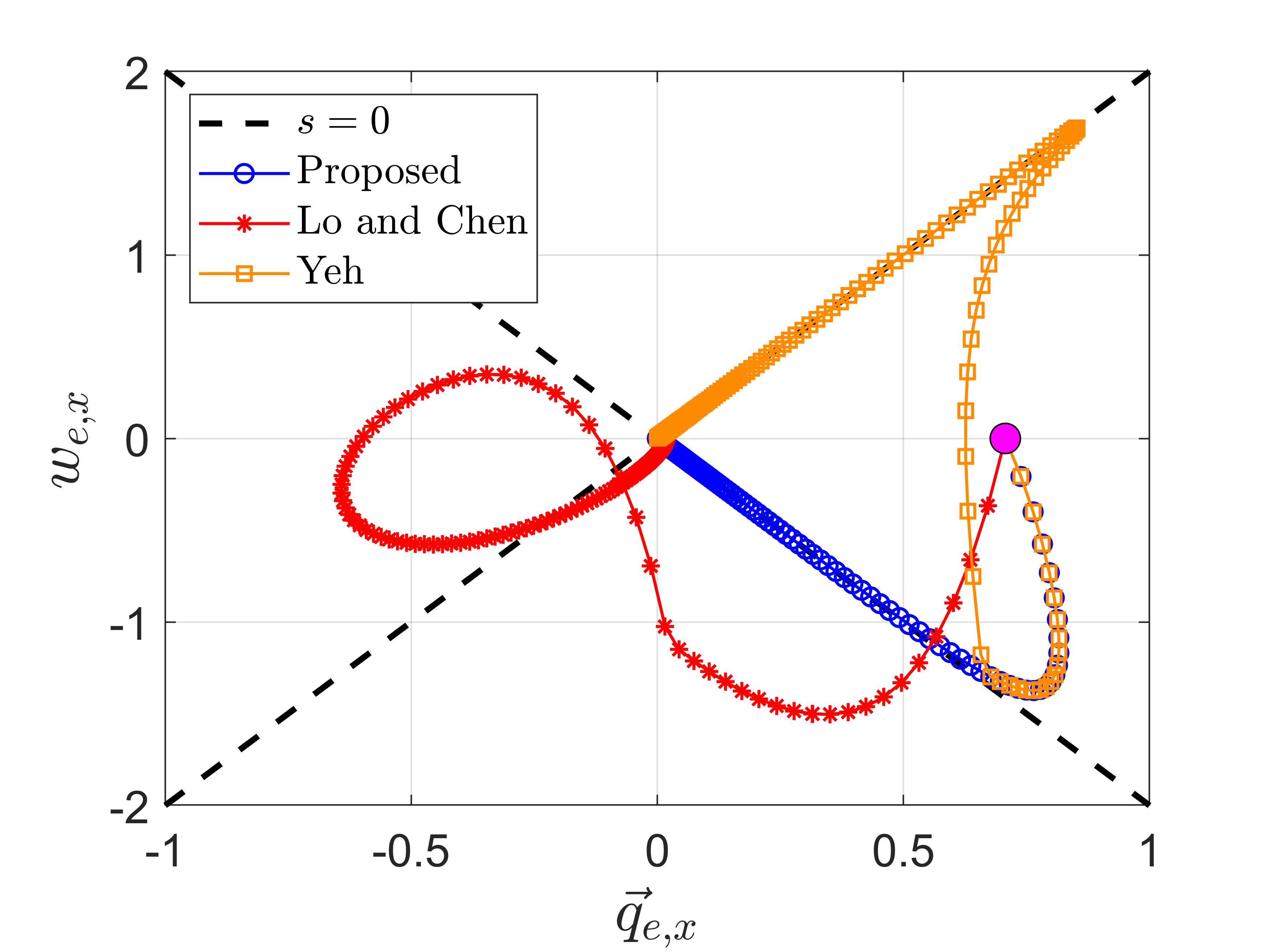
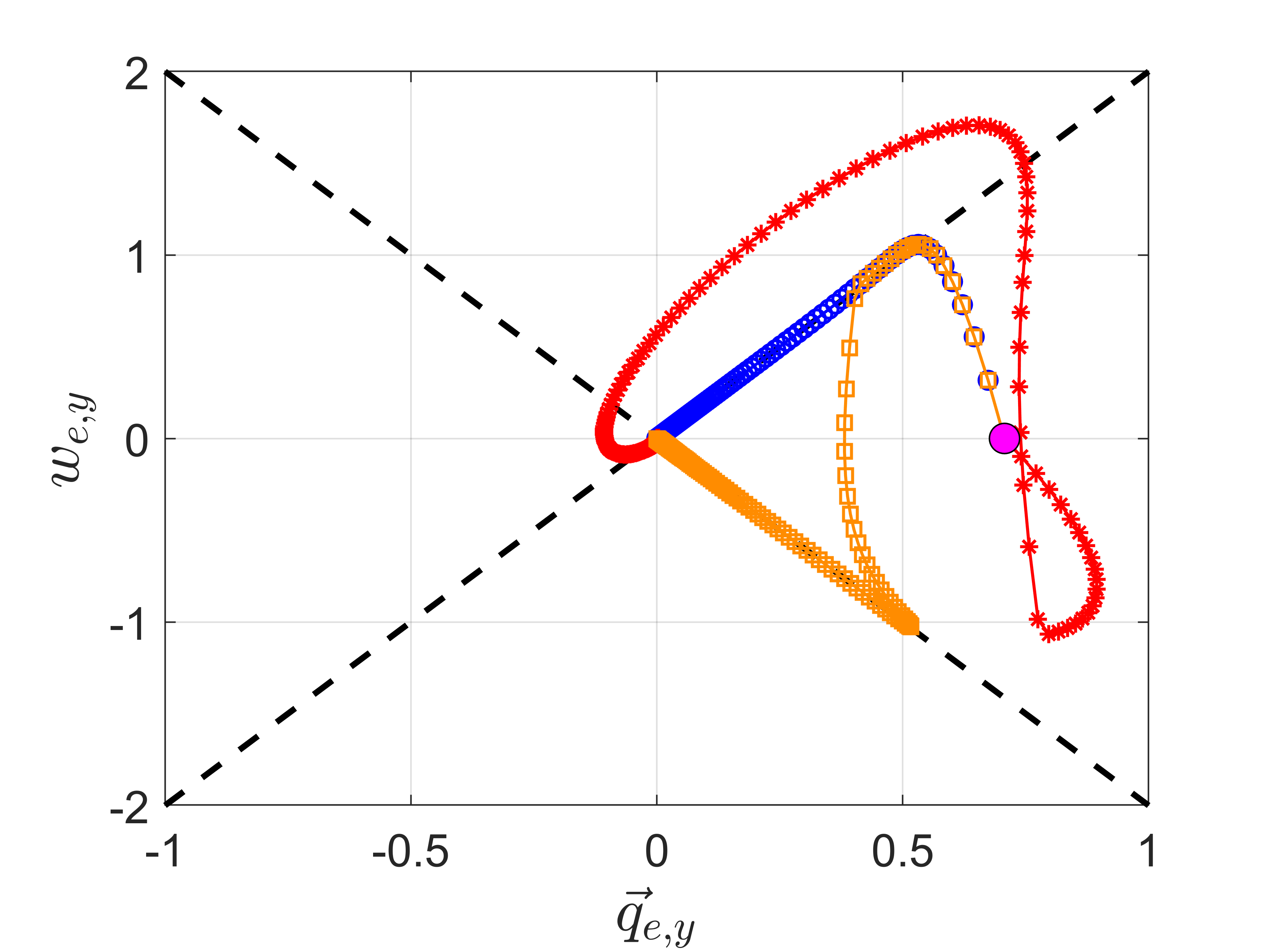
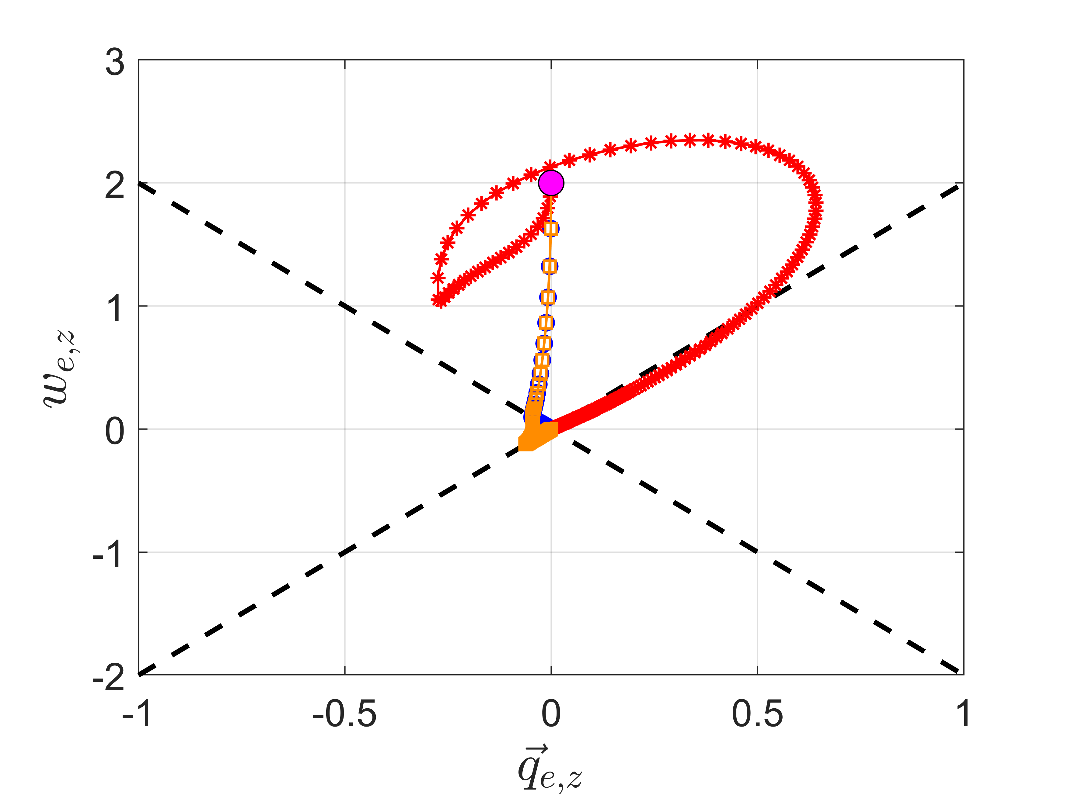
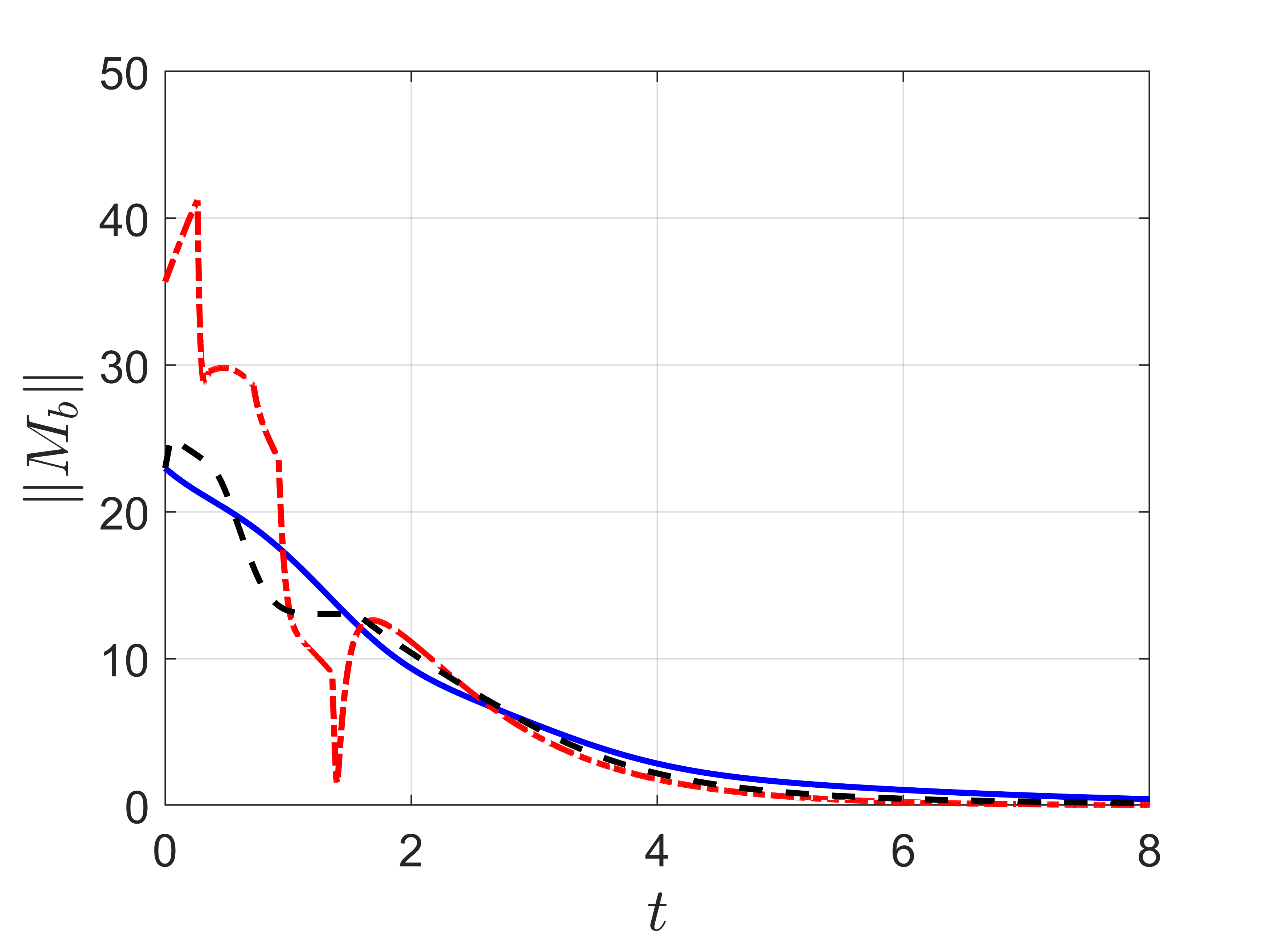
The proposed quaternion sliding variable and the controllers presented in Section IV were compared to other quaternion-based sliding controllers found in the literature. Fig. 3 shows the evolution of the tracking error for the nonlinear PD sliding controller (blue) and those presented in [12, 14] (red and orange) when the quaternion $q$ flips sign midway through an orientation pointing maneuver. Because of the $\mathrm{sgn}_{+}$ term in Equation 3, the sliding surface $\mathcal{S}$ contains two manifolds that correspond to the desired error dynamics. The tracking error with the nonlinear PD controller (blue) exhibits smooth, exponentially convergent behavior despite the sign flip in $q$. The controllers proposed in [12, 14] exhibit poor performance as convergence is slow and unwinding (switching between the two $\mathcal{S}$ manifolds) is observed. Simulation parameters are $J=\mathrm{diag}(10,10,10)$, $f=[0,0,0]^{\top}$, $d=[0.2,-0.2,0.2]^{\top}$, $K=[5,5,5]$, and $\lambda=2$.

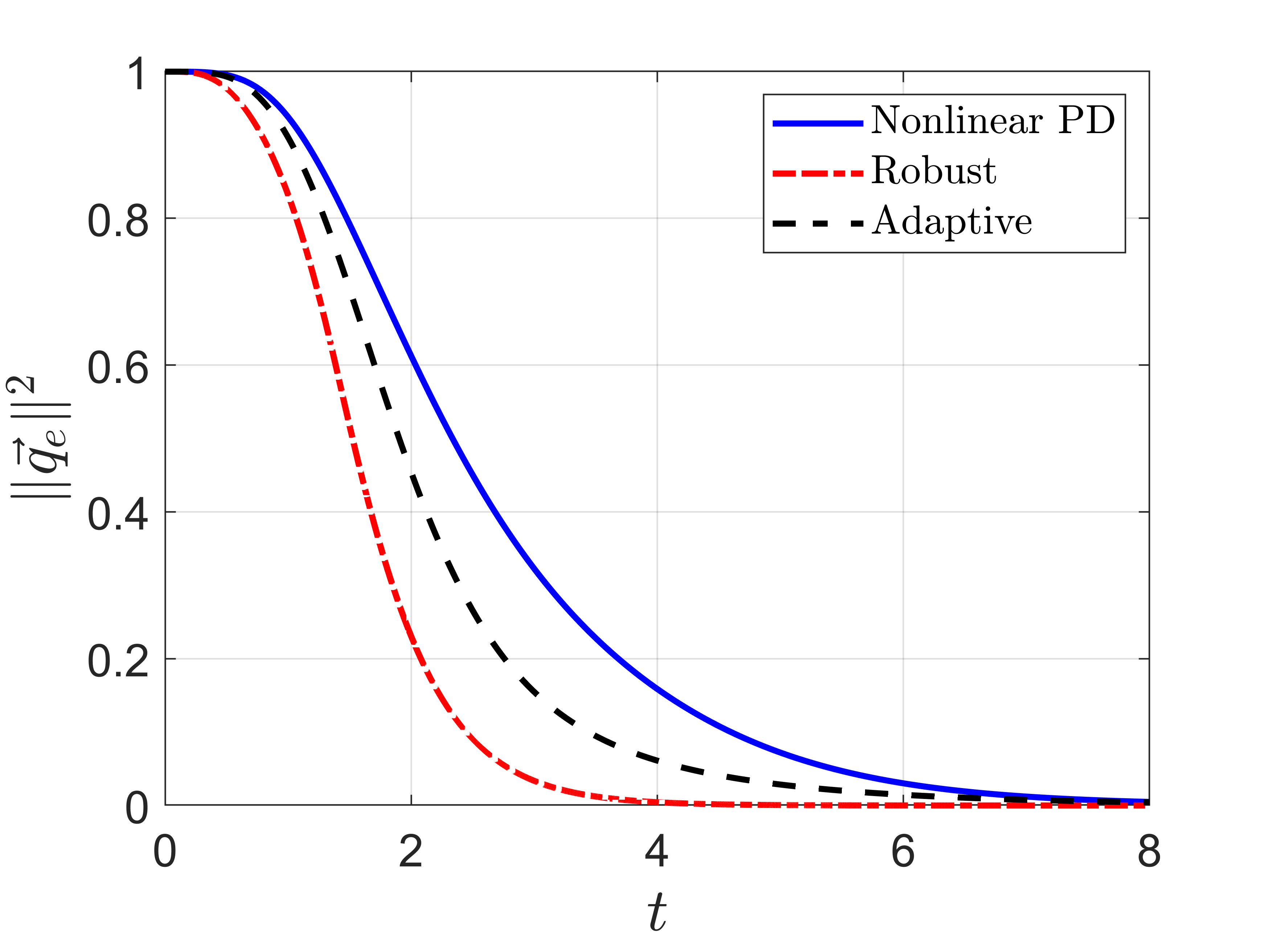
Fig. 4(a) shows the two-norm of the vector part of the error quaternion when the nonlinear PD, robust, and adaptive controller are used to stabilize Equation 1 with uncertainty in the inertia tensor $\mathcal{J}=\mathrm{diag}(3,2,4)$. The boundary layer thickness for Equation 15 is $\Phi=0.1$. The Bregman Divergence with $\psi(x)=\mathrm{log\,det}(x)$ was used to ensure $\hat{J}\succ 0$ during model adaptation. The tracking error with Equation 15 converges faster than that with Equation 20 and Equation 14 but at the expense of larger control effort, shown in Fig. 4(b). Model adaptation can significantly lower control effort while also improving convergence rate when compared to pure nonlinear PD control.

(a) 2-norm of $\vec{q}_{e}$.

(b) 2-norm of control input.

Figure 4: Performance comparison of nonlinear PD, robust, and adaptive sliding control with uncertain inertia tensor. (a): The two norm of $\vec{q}_{e}$ tends toward zero despite model uncertainty for all controllers but convergence rates vary. Robust control outperforms nonlinear PD and adaptive. Model adaptation improves convergence rate of standalone nonlinear PD control. (b) The two norm of $M_{b}$ can become large for the robust controller due to model uncertainty compensation. Using an adaptive control approach lowers control effort at the expense of convergence rate.

VI DISCUSSION

This work presented a quaternion-based sliding variable that represents exponentially convergent quaternion error dynamics. The two defining characteristics of the proposed sliding variable are that it 1) explicitly captures the topology of $\mathbb{S}^{3}$ and 2) contains a benign discontinuity – which actually guarantees the control input is continuous – to eliminate the unwinding behavior. Although several quaternion and $\mathrm{SO(3)}$ controllers have been proposed, the results presented here are easy to analyze, have guaranteed performance, and are straightforward to implement. One research avenue of particular interest is the use of the proposed method for provably safe motion planning of aerial robots flying at high-speeds. Aerodynamic effects can severely degrade the performance of standard attitude controllers making claims on guaranteed safety, i.e., not colliding with obstacles, very difficult to establish. Moreover, the ability to understand how a planned trajectory impacts performance (through time-varying boundary layers), is an element not yet fully leveraged in planning. This, and experimental testing on a physical system, is future work.

References

- [1] T. Lee, M. Leok, and N. H. McClamroch, “Geometric tracking control of a quadrotor uav on se (3),” in 49th IEEE conference on decision and control (CDC), pp. 5420–5425, IEEE, 2010.
- [2] T. Fernando, J. Chandiramani, T. Lee, and H. Gutierrez, “Robust adaptive geometric tracking controls on so (3) with an application to the attitude dynamics of a quadrotor uav,” in 2011 50th IEEE Conference on Decision and Control and European Control Conference, pp. 7380–7385, IEEE, 2011.
- [3] F. Goodarzi, D. Lee, and T. Lee, “Geometric nonlinear pid control of a quadrotor uav on se (3),” in 2013 European control conference (ECC), pp. 3845–3850, IEEE, 2013.
- [4] T. Lee, M. Leok, and N. H. McClamroch, “Nonlinear robust tracking control of a quadrotor uav on se (3),” Asian Journal of Control, vol. 15, no. 2, pp. 391–408, 2013.
- [5] S. P. Bhat and D. S. Bernstein, “A topological obstruction to continuous global stabilization of rotational motion and the unwinding phenomenon,” Systems & Control Letters, vol. 39, no. 1, pp. 63–70, 2000.
- [6] J.-J. E. Slotine, W. Li, et al., Applied nonlinear control, vol. 199. Prentice hall Englewood Cliffs, NJ, 1991.
- [7] B. Wie and P. M. Barba, “Quaternion feedback for spacecraft large angle maneuvers,” Journal of Guidance, Control, and Dynamics, vol. 8, no. 3, pp. 360–365, 1985.
- [8] C. G. Mayhew, R. G. Sanfelice, and A. R. Teel, “Quaternion-based hybrid control for robust global attitude tracking,” IEEE Transactions on Automatic control, vol. 56, no. 11, pp. 2555–2566, 2011.
- [9] E. Fresk and G. Nikolakopoulos, “Full quaternion based attitude control for a quadrotor,” in 2013 European control conference (ECC), pp. 3864–3869, IEEE, 2013.
- [10] C. V. Girish, F. Emilio, H. P. Jonathan, and L. Hugh, “Nonlinear flight control techniques for unmanned aerial vehicles,” in Handbook of Unmanned Aerial Vehicles, pp. 577–612, Springer Netherlands, 2015.
- [11] H. Liu, X. Wang, and Y. Zhong, “Quaternion-based robust attitude control for uncertain robotic quadrotors,” IEEE Transactions on Industrial Informatics, vol. 11, no. 2, pp. 406–415, 2015.
- [12] S.-C. Lo and Y.-P. Chen, “Smooth sliding-mode control for spacecraft attitude tracking maneuvers,” Journal of Guidance, Control, and Dynamics, vol. 18, no. 6, pp. 1345–1349, 1995.
- [13] Y. Jan and J.-C. Chiou, “Minimum-time spacecraft maneuver using sliding-mode control,” Acta Astronautica, vol. 54, no. 1, pp. 69–75, 2004.
- [14] F.-K. Yeh, “Sliding-mode adaptive attitude controller design for spacecrafts with thrusters,” IET control theory & applications, vol. 4, no. 7, pp. 1254–1264, 2010.
- [15] A. Sanchez, V. Parra-Vega, O. Garcia, F. Ruiz-Sanchez, and L. Ramos-Velasco, “Time-parametrization control of quadrotors with a robust quaternion-based sliding mode controller for aggressive maneuvering,” in 2013 European Control Conference (ECC), pp. 3876–3881, IEEE, 2013.
- [16] Y. Zou, “Nonlinear robust adaptive hierarchical sliding mode control approach for quadrotors,” International Journal of Robust and Nonlinear Control, vol. 27, no. 6, pp. 925–941, 2017.
- [17] B. T. Lopez, J.-J. Slotine, and J. P. How, “Robust collision avoidance via sliding control,” in 2018 IEEE International Conference on Robotics and Automation (ICRA), pp. 2962–2969, IEEE, 2018.
- [18] G. C. G. Cortés, F. Castanos, and J. Dávila, “Sliding motions on so (3), sliding subgroups,” in 2019 IEEE 58th Conference on Decision and Control (CDC), pp. 6953–6958, IEEE, 2019.
- [19] P. Culbertson, J.-J. E. Slotine, and M. Schwager, “Decentralized adaptive control for collaborative manipulation of rigid bodies,” arXiv preprint arXiv:2005.03153, 2020.
- [20] Y. Wang, X. Wang, S. Tang, and J. Guo, “Geometric adaptive robust sliding-mode control on so (3).,” in ICINCO (2), pp. 328–338, 2019.
- [21] M. J. Cutler, Design and control of an autonomous variable-pitch quadrotor helicopter. PhD thesis, Citeseer, 2012.
- [22] B. T. Lopez, J. P. How, and J.-J. E. Slotine, “Dynamic tube mpc for nonlinear systems,” in 2019 American Control Conference (ACC), pp. 1655–1662, IEEE, 2019.
- [23] B. T. Lopez, Adaptive robust model predictive control for nonlinear systems. PhD thesis, Massachusetts Institute of Technology, 2019.
- [24] P. M. Wensing, S. Kim, and J.-J. E. Slotine, “Linear matrix inequalities for physically consistent inertial parameter identification: A statistical perspective on the mass distribution,” IEEE Robotics and Automation Letters, vol. 3, no. 1, pp. 60–67, 2017.
- [25] T. Lee, J. Kwon, and F. C. Park, “A natural adaptive control law for robot manipulators,” in 2018 IEEE/RSJ International Conference on Intelligent Robots and Systems (IROS), pp. 1–9, IEEE, 2018.
- [26] N. M. Boffi and J.-J. E. Slotine, “Higher-order algorithms and implicit regularization for nonlinearly parameterized adaptive control,” arXiv, pp. arXiv–1912, 2019.