Estimation, Confidence Intervals, and Large-Scale Hypotheses Testing for High-Dimensional Mixed Linear Regression

This paper studies the high-dimensional mixed linear regression (MLR) where the output variable comes from one of the two linear regression models with an unknown mixing proportion and an unknown covariance structure of the random covariates. Building upon a high-dimensional EM algorithm, we propose an iterative procedure for estimating the two regression vectors and establish their rates of convergence. Based on the iterative estimators, we further construct debiased estimators and establish their asymptotic normality. For individual coordinates, confidence intervals centered at the debiased estimators are constructed.

Furthermore, a large-scale multiple testing procedure is proposed for testing the regression coefficients and is shown to control the false discovery rate (FDR) asymptotically. Simulation studies are carried out to examine the numerical performance of the proposed methods and their superiority over existing methods. The proposed methods are further illustrated through an analysis of a dataset of multiplex image cytometry, which investigates the interaction networks among the cellular phenotypes that include the expression levels of 20 epitopes or combinations of markers.

KEYWORDS: debiasing, EM algorithm, FDR, iterative estimation, large-scale multiple testing

1 INTRODUCTION

Mixed linear regression (MLR) models are widely used in analyzing heterogeneous data arising from biology, physics, economics, and business (McLachlan and Peel 2004; Grün and Leisch 2007; Netrapalli et al. 2013; Li et al. 2019; Devijver et al. 2020). In many of these modern applications, the number of the covariates is comparable with, or sometimes far exceeds, the number of observed samples. In such high-dimensional settings, statistical inference methods designed for estimation and hypothesis testing of the regression coefficients in the classical low-dimensional setting are often not valid. There is a paucity of methods and fundamental theoretical understanding on statistical estimation and inference for high-dimensional MLR models. This motivates us to develop computationally efficient and theoretically guaranteed statistical methods for high-dimensional MLR models in analyzing large heterogeneous datasets.

We consider the following high-dimensional MLR model where the observed data are $i.i.d.$ draws from one of the two unknown linear models:

$$y_{i}=\left\{\begin{array}[]{ll}\bm{x}_{i}^{\top}\bm{\beta}^{*}_{1}+\epsilon_{i}&\textrm{with probability $\omega^{*}$,}\\ \bm{x}_{i}^{\top}\bm{\beta}^{*}_{2}+\epsilon_{i}&\textrm{with probability $1-\omega^{*}$,}\end{array}\right.\quad i=1,2,\ldots,n,\quad\bm{\beta}_{1}^{*},\bm{\beta}_{2}^{*}\in\mathbb{R}^{p},$$ (1.1)

where the random design variables $\bm{x}_{i}\in\mathbb{R}^{p}$ are $i.i.d.$ samples from $N_{p}(0,\mathbb{\Sigma})$ with the unknown covariance matrix $\mathbb{\Sigma}$, $\bm{\beta}^{*}_{1}\neq\bm{\beta}^{*}_{2}$ are latent regression coefficients, $\omega^{*}\in(0,1)$ is the unknown mixing proportion, and the noise $\epsilon_{i}$ is $i.i.d.$ from $N(0,\sigma^{2})$ for some $\sigma>0$. For identifiability, we assume $\omega^{*}\in(1/2,1)$. Under the high-dimensional setting where $p$ is much larger than $n$, we aim to answer the following inference questions:

1. What is an efficient algorithm for estimating the underlying regression vectors $\bm{\beta}_{1}^{*}$ and $\bm{\beta}_{2}^{*}$ where both the mixing proportion $\omega^{*}$ and the random design covariance matrix $\mathbb{\Sigma}$ are unknown? What is the rate of convergence of the estimator?

2. How to construct asymptotically valid tests and confidence intervals for the individual coordinates of the latent regression coefficients $\bm{\beta}^{*}_{1}$ and $\bm{\beta}_{2}^{*}$, and their difference $\bm{\beta}^{*}_{1}-\bm{\beta}_{2}^{*}$?

3. For simultaneously testing the null hypotheses $H_{0j}:\bm{\beta}_{1j}^{*}=\bm{\beta}_{2j}^{*}=0$, $j=1,...,p$, how to construct a large-scale multiple testing procedure that controls the false discovery rate (FDR) and false discovery proportion (FDP) asymptotically?

1.1 Related Works

In the classical low-dimensional settings, the problems of estimation, hypotheses testing and confidence intervals for MLR have been extensively studied in literature. For example, Zhu and Zhang (2004) considered hypothesis testing and developed an asymptotic theory for both the maximum likelihood and the maximum modified likelihood estimators in MLR. Khalili and Chen (2007) introduced a penalized likelihood approach for variable selection in MLR. Faria and Soromenho (2010) compared three expectation-maximization (EM) algorithms that compute the maximum likelihood estimates of the coefficients of MLR. Chaganty and Liang (2013) developed a computationally efficient algorithm based on the tensor power method, and obtained the rates of convergence for their proposed estimator. Bashir and Carter (2012) proposed a robust model that can achieve high breakdown point in the contaminated data for parameter estimation in MLR. Based on a new initialization step for the EM algorithm, Yi et al. (2014) provided the theoretical guarantees for coefficient estimation in MLR. Moreover, Yao and Song (2015) proposed a deconvolution method to study the MLR with measurement errors. Zhong et al. (2016) proposed a non-convex continuous objective function for solving the general unbalanced $k$-component MLR.

Balakrishnan et al. (2017) developed a general framework for proving rigorous guarantees on the performance of the EM algorithm and applied to some statistical problems including the estimation of coefficients in the symmetric MLR where the mixing proportion is known to be $\omega^{*}=1/2$. Li and Liang (2018) presented a fixed parameter algorithm that solves MLR under Gaussian design in time that is nearly linear in the sample size and the dimension. More recently, building upon the work of Balakrishnan et al. (2017) on the symmetric MLR, McLachlan and Peel (2004) and Klusowski et al. (2019) introduced better tools for analyzing the convergence rates of the EM algorithm for estimating the coefficients. Shen and Sanghavi (2019) proposed an efficient algorithm, Iterative Least Trimmed Squares, for solving MLR with adversarial corruptions.

In contrast, statistical inference for MLR in the high-dimensional setting is relatively less studied. Specifically, Städler et al. (2010) proposed an $\ell_{1}$ penalized estimator and developed an efficient EM algorithm for MLR with provable convergence properties. Wang et al. (2015) and Yi and Caramanis (2015) established a general theory of the EM algorithm for statistical inference in high dimensional latent variable models, including the high-dimensional MLR with the symmetric and spherical assumptions. In Zhu et al. (2017), a generic stochastic EM algorithm was proposed for the high-dimensional MLR with theoretical guarantees obtained under the symmetric setting ($\omega^{*}=1/2$). More recently, Fan et al. (2018) studied the fundamental tradeoffs between statistical accuracy and computational tractability for high-dimensional latent variables models, including testing the global null hypothesis in MLR. However, problems such as statistical inference about the individual regression coefficients and large-scale multiple testing under the general MLR with an unknown mixing proportion and an unknown design covariance matrix have not been addressed in the literature.

1.2 Main Contributions

The main contributions of our paper are three-fold.

1. Based on a careful analysis of a high-dimensional EM algorithm, we propose iterative estimators for the regression coefficients $(\bm{\beta}_{1}^{*},\bm{\beta}_{2}^{*})$ without the knowledge of the mixing proportions or the design covariance matrix, and obtain explicitly the rates of convergence of the iterative estimators under the $\ell_{2}$ norm. To the best of our knowledge, this is the first result on the estimation of the high-dimensional MLR with both unknown mixing proportion and unknown design covariance matrix.

2. Further, we construct debiased estimators of the latent regression coefficients, based on the iterative estimators, and establish the asymptotic normality of its individual coordinates. The limiting distribution is then used for constructing confidence intervals and tests for the individual latent regression coefficients.

3. For the problem of large-scale testing of hypotheses $H_{0j}:\bm{\beta}_{1j}^{*}=\bm{\beta}_{2j}^{*}=0$, $j=1,...,p$, we propose a multiple testing procedure that is shown to control the FDR and FDP asymptotically. Strong numerical results suggest the superior empirical performance of our proposed testing procedure over the existing methods.

1.3 Organization and Notation

Throughout our paper, for a vector $\mathbb{a}=(a_{1},...,a_{n})^{\top}\in\mathbb{R}^{n}$, we define the $\ell_{p}$ norm $\|\mathbb{a}\|_{p}=\big{(}\sum_{i=1}^{n}a_{i}^{p}\big{)}^{1/p}$, and the $\ell_{\infty}$ norm $\|\mathbb{a}\|_{\infty}=\max_{1\leq j\leq n}|a_{i}|$. $\mathbb{a}_{-j}\in\mathbb{R}^{n-1}$ stands for the subvector of $\mathbb{a}$ without the $j$-th component. For vectors $\mathbb{a},\mathbb{b}\in\mathbb{R}^{n}$, we denote their inner product $\langle\mathbb{a},\mathbb{b}\rangle=\sum_{i=1}^{n}a_{i}b_{i}$. For a matrix $A\in\mathbb{R}^{p\times q}$, $\lambda_{i}(A)$ stands for the $i$-th largest singular value of $A$ and $\lambda_{\max}(A)=\lambda_{1}(A)$, $\lambda_{\min}(A)=\lambda_{p\wedge q}(A)$. $\|A\|_{1}$ denotes the matrix $\ell_{1}$ norm, and $\|A\|_{\infty}=\max_{i,j}|A_{ij}|$. In addition, $A_{-i.-j}\in\mathbb{R}^{(p-1)\times(q-1)}$ stands for the submatrix of $A$ without the $i$ th row and $j$-th column. For any positive integer $p$, we denote $[p]=\{1,...,p\}$. Furthermore, for sequences $\{a_{n}\}$ and $\{b_{n}\}$, we write $a_{n}=o(b_{n})$ if $\lim_{n}a_{n}/b_{n}=0$, and write $a_{n}=O(b_{n})$, $a_{n}\lesssim b_{n}$ or $b_{n}\gtrsim a_{n}$ if there exists a constant $C$ such that $a_{n}\leq Cb_{n}$ for all $n$. We also write $a_{n}=O_{P}(b_{n})$ if there exists a constant $C$ such that $\lim\inf_{n\to\infty}\mathbb{P}(a_{n}\leq Cb_{n})=1$, and $a_{n}=o_{P}(b_{n})$ if $a_{n}/b_{n}\stackrel{{\scriptstyle p}}{{\to}}1$. We write $a_{n}\asymp b_{n}$ if $a_{n}\lesssim b_{n}$ and $a_{n}\gtrsim b_{n}$. For a set $A$, we denote $|A|$ as its cardinality. Lastly, $C,C_{0},C_{1},...$ are constants that may vary from place to place.

The rest of the paper is organized as follows. We propose in Section 2 the iterative algorithm and the estimators of the latent regression coefficients and study their theoretical properties. Section 3 introduces the debiased estimators of individual regression coefficients and obtains their asymptotic normality and the resulting confidence intervals. In Section 4, by focusing on the problem of testing large-scale simultaneous hypotheses, we present our multiple testing procedure and show that it controls the FDR/FDP asymptotically. In Section 5, the numerical performance of the proposed methods are evaluated through extensive simulations. In Section 6, the proposed procedures are illustrated by an analysis of a multiplex image cytometry dataset. Further extensions and related problems are discussed in Section 7. The proofs of other theorems as well as technical lemmas are collected in the Supplementary Materials (Zhang et al. 2020).

2 ITERATIVE ESTIMATION VIA THE EM ALGORITHM

Suppose we have $n$ observations $\{(\bm{x}_{i},y_{i})\}_{i=1}^{n}$ generated independently from the MLR model in (1.1), and wish to estimate and make inference on the coefficient vectors $\bm{\beta}_{1}^{*}$ and $\bm{\beta}_{2}^{*}$. In the classical setting where $p$ is fixed or much smaller than $n$, the maximum likelihood estimator (MLE) has been shown to perform well under mild conditions (Balakrishnan et al. 2017). The MLE aims to maximize the log-likelihood of the data $\{(\bm{x}_{i},y_{i})\}_{i=1}^{n}$, which can be written as

$$l_{n}(\bm{\theta};\bm{x},y)=\frac{1}{n}\sum_{i=1}^{n}\log\bigg{[}\frac{\omega}{\sqrt{2\pi}\sigma}\exp\left\{{-\frac{(y_{i}-\langle\bm{x}_{i},\bm{\beta}_{1}\rangle)^{2}}{2\sigma^{2}}}\right\}+\frac{1-\omega}{\sqrt{2\pi}\sigma}\exp\left\{{-\frac{(y_{i}-\langle\bm{x}_{i},\bm{\beta}_{2}\rangle)^{2}}{2\sigma^{2}}}\right\}\bigg{]},$$ (2.1)

where we denote the parameter $\bm{\theta}=(\omega,\bm{\beta}_{1},\bm{\beta}_{2})$ and the log-likelihood by $l_{n}(\bm{\theta})$.

Due to the non-convexity of $l_{n}(\bm{\theta};\bm{x},y)$, searching for the MLE is computationally intractable. Moreover, in the high-dimensional setting where the dimension $p$ is much larger than the sample size $n$, the MLE is in general not well defined, unless the models are carefully regularized by sparsity-type assumptions. In this paper, we propose to explore the sparsity of the coefficient vectors. Further, we develop an EM algorithm to address the extra computational challenge for parameter estimation and uncertainty assessment.

2.1 High-Dimensional EM Algorithm and the Iterative Estimators

For ease of presentation, let us use $z_{i}$ to denote the hidden labels of $(\bm{x}_{i},y_{i})$, that is, $z_{i}=1$ if $(\bm{x}_{i},y_{i})$ is drawn from the first model $y_{i}=\bm{x}_{i}^{\top}\bm{\beta}_{1}^{*}+\epsilon_{i}$, and $z_{i}=2$ if the underlying truth is the second model $y_{i}=\bm{x}_{i}^{\top}\bm{\beta}_{2}^{*}+\epsilon_{i}$. The marginal distribution of $z_{i}$ is given by $\mathbb{P}(z_{i}=1)=1-\mathbb{P}(z_{i}=2)=\omega$. The EM algorithm is essentially an alternating maximization method, which alternatively optimizes between the identification of hidden labels $\{z_{i}\}_{i=1}^{n}$ and the estimation of parameter $\bm{\theta}=(\omega,\bm{\beta}_{1},\bm{\beta}_{2})$.

Specifically, in the E-step of $(t+1)$-th iteration, given the parameters $\bm{\theta}^{(t)}=(\omega^{(t)},\bm{\beta}_{1}^{(t)},\bm{\beta}_{2}^{(t)})$ estimated from the previous $t$-th step, the conditional probability of the $i$-th sample in class 1 given the observed data $(\bm{x}_{i},y_{i})$ can be calculated as

$$\gamma_{\bm{\theta}^{(t)}}(\bm{x}_{i},y_{i}):=\mathbb{P}_{\bm{\theta}^{(t)}}(z_{i}=1\mid\bm{x}_{i},y_{i})=\frac{\omega^{(t)}\exp(-\frac{(y_{i}-\langle\bm{x}_{i},\bm{\beta}_{1}^{(t)}\rangle)^{2}}{2\sigma^{2}})}{\omega^{(t)}\exp(-\frac{(y_{i}-\langle\bm{x}_{i},\bm{\beta}^{(t)}_{1}\rangle)^{2}}{2\sigma^{2}})+(1-\omega^{(t)})\exp(-\frac{(y_{i}-\langle\bm{x}_{i},\bm{\beta}_{2}^{(t)}\rangle)^{2}}{2\sigma^{2}})}.$$ (2.2)

As a result, the conditional expectation of the log-likelihood (2.1), with respect to the conditional distribution given $(\bm{x},y)$ under the current estimate of the parameter $\bm{\theta}^{(t)}$, can be calculated as

$$Q_{n}(\bm{\theta}\mid\bm{\theta}^{(t)}):= \mathbb{E}_{\bm{\theta}^{(t)}}[l_{n}(\bm{\theta};\bm{x},y)\mid\bm{x},y]$$ (2.3)

$$= -\frac{1}{2n}\left[\sum_{i=1}^{n}\gamma_{\bm{\theta}^{(t)}}(\bm{x}_{i},y_{i})(y_{i}-\langle\bm{x}_{i},\bm{\beta}_{1}\rangle)^{2}+\sum_{i=1}^{n}(1-\gamma_{\bm{\theta}^{(t)}}(\bm{x}_{i},y_{i}))(y_{i}-\langle\bm{x}_{i},\bm{\beta}_{2}\rangle)^{2}\right]$$

$$+\frac{1}{n}\sum_{i=1}^{n}(1-\gamma_{\bm{\theta}^{(t)}}(\bm{x}_{i},y_{i}))\log(1-\omega)+\gamma_{\bm{\theta}^{(t)}}(\bm{x}_{i},y_{i})\log\omega.$$

Given $\gamma_{\bm{\theta}^{(t)}}(\bm{x}_{i},y_{i})$, i.e., the distribution of the latent labels, the M-step is usually proceeded by maximizing $Q_{n}(\bm{\theta}\mid\bm{\theta}^{(t)})$:

$$\hat{\bm{\theta}}^{(t+1)}=\mathop{\rm arg\max}_{\bm{\theta}}Q_{n}(\bm{\theta}\mid\bm{\theta}^{(t)}).$$

However, in the high-dimensional setting, such a maximization tends to overfit data. To handle the challenge of high-dimensionality, the key ingredient of our algorithm is to add a regularization term $\|\bm{\beta}\|_{1}$ to enforce sparsity. In particular, we write $\gamma^{(t)}_{\bm{\theta},i}=\gamma_{\bm{\theta}^{(t)}}(\bm{x}_{i},y_{i})$, and let

$$\hat{\bm{\beta}}_{1}^{(t+1)} =\mathop{\rm arg\min}_{\bm{\beta}_{1}}\frac{1}{2n}\sum_{i=1}^{n}\gamma^{(t)}_{\bm{\theta},i}(y_{i}-\langle\bm{x}_{i},\bm{\beta}_{1}\rangle)^{2}+\lambda_{n}^{(t+1)}\|\bm{\beta}_{1}\|_{1}$$ (2.4)

$$\hat{\bm{\beta}}_{2}^{(t+1)} =\mathop{\rm arg\min}_{\bm{\beta}_{2}}\frac{1}{2n}\sum_{i=1}^{n}(1-\gamma^{(t)}_{\bm{\theta},i})(y_{i}-\langle\bm{x}_{i},\bm{\beta}_{2}\rangle)^{2}+\lambda_{n}^{(t+1)}\|\bm{\beta}_{2}\|_{1},$$

where $\lambda^{(t+1)}$ is a tuning parameter which will also be updated recursively, and will be specified later. We also update $\omega^{(t+1)}$ by

$$\omega^{(t+1)}=\frac{1}{n}\sum_{i=1}^{n}\gamma_{\bm{\theta}^{(t)}}(\bm{x}_{i},y_{i}).$$

Given a suitable initialization, the proposed high-dimensional EM algorithm then proceeds by iterating between the E-step and the M-step, which is summarized in the following Algorithm 1.

Algorithm 1 EM for High-Dimensional MLR

1:Inputs: Initializations $\hat{\omega}^{(0)},\hat{\bm{\beta}}_{1}^{(0)},\hat{\bm{\beta}}_{2}^{(0)}$, maximum number of iterations $T$, and constants $\kappa\in(0,1)$, $C_{\lambda}>0$. Split the Dataset into $T$ subsets of size $n/T$. For $i\in[n]$, set

$$\gamma^{(0)}_{\bm{\theta},i}=\frac{\hat{\omega}^{(0)}\exp(-\frac{(y_{i}-\langle\bm{x}_{i},\hat{\bm{\beta}}^{(0)}_{1}\rangle)^{2}}{2\sigma^{2}})}{\hat{\omega}^{(0)}\exp(-\frac{(y_{i}-\langle\bm{x}_{i},\hat{\bm{\beta}}^{(0)}_{1}\rangle)^{2}}{2\sigma^{2}})+(1-\hat{\omega}^{(0)})\exp(-\frac{(y_{i}-\langle\bm{x}_{i},\hat{\bm{\beta}}^{(0)}_{2}\rangle)^{2}}{2\sigma^{2}})}.$$

2:for $t=0,1,\ldots,T-1$ do

3:     E-Step: Evaluate $Q_{n}(\bm{\theta}\mid\hat{\bm{\theta}}^{(t)})$ as defined in (2.3) with the $t$-th data subset.

4:     M-Step: Update $\bm{\beta}_{1}^{(t+1)}$ and $\hat{\bm{\beta}}^{(t+1)}$ via

$$\hat{\bm{\beta}}_{1}^{(t+1)} =\mathop{\rm arg\min}_{\bm{\beta}_{1}}\frac{1}{2n}\sum_{i=1}^{n}\gamma^{(t)}_{\bm{\theta},i}(y_{i}-\langle\bm{x}_{i},\bm{\beta}_{1}\rangle)^{2}+\lambda_{n}^{(t+1)}\|\bm{\beta}_{1}\|_{1}$$ (2.5)

$$\hat{\bm{\beta}}_{2}^{(t+1)} =\mathop{\rm arg\min}_{\bm{\beta}_{2}}\frac{1}{2n}\sum_{i=1}^{n}(1-\gamma^{(t)}_{\bm{\theta},i})(y_{i}-\langle\bm{x}_{i},\bm{\beta}_{2}\rangle)^{2}+\lambda_{n}^{(t+1)}\|\bm{\beta}_{2}\|_{1},$$

with

$$\lambda_{n}^{(t+1)}=\kappa_{\lambda}\lambda_{n}^{(t)}+C_{\lambda}\sqrt{\frac{\log p}{n}}.$$ (2.6)

Update $\hat{\omega}^{(t)}$ via $\hat{\omega}^{(t)}=\frac{1}{n}\sum_{i=1}^{n}\gamma^{(t)}_{\bm{\theta},i}.$

5:end for

6:Output $\bm{\beta}_{1}^{(T)}$ and $\hat{\bm{\beta}}_{2}^{(T)}$.

Remark 1.

In the above algorithm, it is required that the noise level $\sigma^{2}$ is known. Such an assumption is widely used in prior literature in mixed linear regressions, see Wang et al. (2015); Balakrishnan et al. (2017); Klusowski et al. (2019) and reference therein. In practice, a good estimator of $\sigma^{2}$ can be substituted in the algorithm to achieve deisrable empirical performance. See Section 5 for more detailed numerical justifications.

2.2 Rate of Convergence

In this section, we give theoretical guarantees for estimating the coefficient vectors $\bm{\beta}_{1}^{*}$ and $\bm{\beta}_{2}^{*}$ using Algorithm 1. To begin with, we introduce the parameter space for $(\omega^{*},\bm{\beta}_{1}^{*},\bm{\beta}_{2}^{*})$, where we assume that $\bm{\beta}_{1}^{*}$ and $\bm{\beta}_{2}^{*}$ are both sparse vectors and $\omega^{*}$ is bounded away from 0 or 1.

$$\Theta(s)=\bigg{\{}(\omega,\bm{\beta}_{1},\bm{\beta}_{2}):\omega\in(c,1-c),\|\bm{\beta}_{1}\|_{0},\|\bm{\beta}_{2}\|_{0}\leq s,\text{ for some }c\in(0,1/2)\bigg{\}}.$$

Furthermore, we introduce the following regularity conditions on the initialization and signal-to-noise ratio (SNR) strength.

• : Initialization: $\|\bm{\beta}_{1}^{(0)}-\bm{\beta}_{1}^{*}\|_{2}+\|\bm{\beta}_{2}^{(0)}-\bm{\beta}_{2}^{*}\|+|\omega^{(0)}-\omega^{*}|\leq\min\{\omega^{*}/2,(1-\omega^{*})/2,c_{l}\cdot{\Delta^{*}}\}$, where $\Delta^{*}=\sqrt{(\bm{\beta}_{1}^{*}-\bm{\beta}_{2}^{*})^{\top}\mathbb{\Sigma}^{-1}(\bm{\beta}_{1}^{*}-\bm{\beta}_{2}^{*})}$;

• : SNR strength: $(\bm{\beta}_{1}^{*}-\bm{\beta}_{2}^{*})^{\top}\mathbb{\Sigma}^{-1}(\bm{\beta}_{1}^{*}-\bm{\beta}_{2}^{*})\geq c_{s}$,

where $c_{l},c_{s}>0$ are some universal constants that and do not grow with $n$ or $p$. The (A1) suggests the initialized estimator should be closed to the truth. Such a condition is common in the literature of mixed linear regression, see Balakrishnan et al. (2017); Yi et al. (2014); Wang et al. (2015); Yi and Caramanis (2015). In practice, our initialization algorithm is discussed in Section 5. Condition (A2) has also been commonly used in the literature of mixed linear regression (Balakrishnan et al. 2017; Klusowski et al. 2019), and other hidden variable models (Wang et al. 2015; Cai et al. 2019).

Theorem 1.

Suppose $1/M<\lambda_{\min}(\mathbb{\Sigma})\leq\lambda_{\max}(\mathbb{\Sigma})<M$ for some constant $M>1$ and conditions (A1) and (A2) hold. If $\frac{s\log p{\cdot\log n}}{n}=o(1)$, and $c_{l}$ is sufficiently large, that is, $c_{l}\geq C(\omega^{*},M,c_{l})$ where $C(\omega^{*},M,c_{l})$ is a constant depending only on $(\omega^{*},M,c_{l})$. Then $T\gtrsim\log n$, we have with probability at least $1-p^{-1}$,

$$\|\hat{\bm{\beta}}_{1}^{(T)}-\bm{\beta}_{1}^{*}\|_{2}+\|\hat{\bm{\beta}}_{2}^{(T)}-\bm{\beta}_{2}^{*}\|_{2}\lesssim\sqrt{\frac{s\log p{\cdot\log n}}{n}}.$$

Remark 2.

The condition on the spectrum of $\mathbb{\Sigma}$ is standard in the high-dimensional literature. For example, it has been used in Cai et al. (2016); Cai and Zhou (2012) and Javanmard and Montanari (2014a) for estimation of precision matrices, covariance matrices and regression coefficients, respectively. Further, the convergence rate of optimization error is exponentially fast, so we only need that the number of iterations $T\gtrsim\log n$ to make the optimization error negligible comparing to the statistical error.

3 DEBIASED ESTIMATORS AND THEIR ASYMPTOTIC NORMALITY

The iterative estimators obtained from the high-dimensional EM algorithm (Algorithm 1) enjoys desirable properties in term of squared error, they are however unsuitable to be used directly for statistical inference. In this section, we introduce the debiased estimators for the mixed linear regression coefficients $\bm{\beta}^{*}_{\ell j}$ with $\ell\in\{1,2\}$ and $j\in[p]$, and obtain their asymptotic normality, which can then be used to perform hypothesis testing and construct confidence intervals for the individual coefficients.

3.1 Debiased Estimators

Due to the $\ell_{1}$ regularization in the M-step, the outputs $\hat{\bm{\beta}}_{1}^{(T)}$ and $\hat{\bm{\beta}}_{2}^{(T)}$ from the high-dimensional EM algorithm (Algorithm 1) are biased. To facilitate the subsequent statistical inference, we proceed by correcting their biases. Such a de-biased procedure has been used widely in high-dimensional single linear regression models (Javanmard and Montanari 2014a, b; van de Geer et al. 2014; Zhang and Zhang 2014; Ning and Liu 2017), but cannot be directly applied to the EM solutions. In the following, we first present some high-level intuition.

We start with the regression coefficient $\bm{\beta}^{*}_{1}$. Note that in Algorithm 1, $\hat{\bm{\beta}}_{1}^{(T)}$ is constructed only based on the $T$-th sample, and the sample size is $n/T$ with $T\asymp\log n$. In the following, for the notational simplicity, we simply write $n_{T}=n/T$. Firstly, $\hat{\bm{\beta}}_{1}^{(T)}$ satisfies the Karush-Kuhn-Tucker (KKT) condition

$$-\frac{1}{n}\sum_{i=1}^{n_{T}}\gamma_{\bm{\theta},i}^{(T)}(y_{i}-\langle\bm{x}_{i},\hat{\bm{\beta}}_{1}^{(T)}\rangle)\bm{x}_{i}+\lambda_{n}^{(T)}\partial||\hat{\bm{\beta}}_{1}^{(T)}||_{1}=0,$$ (3.1)

where $\partial||\hat{\bm{\beta}}_{1}^{(T)}||_{1}$ is the subgradient of the $\ell_{1}$ norm $||\cdot||_{1}$. Letting $\widehat{\Sigma}_{XX}=\frac{1}{n_{T}}\sum_{i=1}^{n_{T}}\gamma_{\bm{\theta},i}^{(T)}\bm{x}_{i}\bm{x}_{i}^{\top}$ and $\widehat{\Sigma}_{XY}=\frac{1}{n_{T}}\sum_{i=1}^{n_{T}}\gamma_{\bm{\theta},i}^{(T)}\bm{x}_{i}y_{i}$, equation (3.1) can then be rewritten as

$$\widehat{\Sigma}_{XX}\hat{\bm{\beta}}_{1}^{(T)}-\widehat{\Sigma}_{XY}+\lambda_{n}^{(T)}\partial||\hat{\bm{\beta}}_{1}^{(T)}||_{1}=0,$$

and as a result,

$$\widehat{\Sigma}_{XX}(\hat{\bm{\beta}}_{1}^{(T)}-\bm{\beta}_{1}^{*})+\lambda_{n}^{(T)}\partial||\hat{\bm{\beta}}_{1}^{(T)}||_{1}=\widehat{\Sigma}_{XY}-\widehat{\Sigma}_{XX}\bm{\beta}_{1}^{*}.$$

Following the debiased Lasso method in Javanmard and Montanari (2014a), suppose one has a good approximation of the “inverse” of $\widehat{\Sigma}_{XX}$, say $M$, then one can multiply $M$ on the left to obtain

$$M\widehat{\Sigma}_{XX}(\hat{\bm{\beta}}_{1}^{(T)}-\bm{\beta}_{1}^{*})+\lambda_{n}^{(T)}M\partial||\hat{\bm{\beta}}_{1}^{(T)}||_{1}=M(\widehat{\Sigma}_{XY}-\widehat{\Sigma}_{XX}\bm{\beta}_{1}^{*}).$$

Then it follows

$$(\hat{\bm{\beta}}_{1}^{(T)}+\lambda_{n}^{(T)}M\partial||\hat{\bm{\beta}}_{1}^{(T)}||_{1})-\bm{\beta}_{1}^{*}=M(\widehat{\Sigma}_{XY}-\widehat{\Sigma}_{XX}\bm{\beta}_{1}^{*})+(I-M\widehat{\Sigma}_{XX})(\hat{\bm{\beta}}_{1}^{(T)}-\bm{\beta}_{1}^{*}).$$ (3.2)

By inspection, if we let $\widehat{\bm{\beta}}_{1}^{u}=\hat{\bm{\beta}}_{1}^{(T)}+\lambda_{n}^{(T)}M\partial||\hat{\bm{\beta}}_{1}^{(T)}||_{1}$, then

$$\sqrt{n}(\widehat{\bm{\beta}}_{1}^{u}-\bm{\beta}_{1}^{*})= \sqrt{n}(M\widehat{\Sigma}_{XY}-M\widehat{\Sigma}_{XX}{\bm{\beta}_{1}^{*}})+\sqrt{n}(I-M\widehat{\Sigma}_{XX})(\hat{\bm{\beta}}_{1}^{(T)}-{\bm{\beta}}_{1}^{*})$$

$$= \sqrt{n}\bigg{[}\frac{1}{n}\sum_{i=1}^{n}\gamma_{\bm{\theta},i}^{(T)}(y_{i}-\langle\bm{x}_{i},\bm{\beta}_{1}^{*}\rangle)M\bm{x}_{i}\bigg{]}+o_{P}(1),$$

where the second equality incorporated the assumption that $M$ approximate the “inverse” of $\widehat{\Sigma}_{XX}$ well and thus $\|(I-M\widehat{\Sigma}_{XX})(\hat{\bm{\beta}}_{1}^{(T)}-\bm{\beta}_{1}^{*})\|_{\infty}\leq\|I-M\widehat{\Sigma}_{XX}\|_{\infty}\|\hat{\bm{\beta}}_{1}^{(T)}-\bm{\beta}_{1}^{*}\|_{1}$ is negligible.

Unlike the procedure in Javanmard and Montanari (2014a), our $\hat{\Sigma}_{XX}$ depends on $(\bm{x}_{i},y_{i})$ instead of only on $\bm{x}_{i}$’s, and therefore solving a direct approximation will mess up with the subsequent asymptotic normality. We propose to solve $M$ by the following two-step procedure. First, let $\tilde{\Sigma}_{XX}=\frac{1}{n}\sum_{i=1}^{n}\bm{x}_{i}\bm{x}_{i}^{\top}$, for $j\in[p]$, let $\bm{\tilde{m}}_{j}$ be the solution of

$$\underset{\bm{m}_{j}\in\mathbb{R}^{p}}{\text{minimize}} \bm{m}_{j}^{\top}\hat{\Sigma}_{XX}\bm{m}_{j}$$ (3.3)

subject to $$||\hat{\Sigma}_{XX}\bm{m}_{j}-e^{(p)}_{j}||_{\infty}\leq\mu,$$

$$\|\bm{m}_{j}\|\leq C\sqrt{\log n}.$$

where $\mu$ and $C$ are tuning parameters that will be discussed later.

Second we set $\bm{m}_{j}=\bm{\tilde{m}}_{j}/\hat{\omega}^{(T)},$ with $\hat{\omega}^{(T)}=\hat{\omega}^{(T)}\frac{1}{n}\sum_{i=1}^{n}\gamma_{\bm{\theta},i}^{(T)}$. The denominator is used because $\tilde{\Sigma}_{XX}$ is approximately $\omega^{*}\cdot\hat{\Sigma}_{XX}$. Although $\hat{\omega}^{(T)}$ still depends on $(\bm{x}_{i},y_{i})$, but it is close to $\omega^{*}$ and the distance is negligible.

Now, to find the asymptotic distribution of $\sqrt{n_{T}}(\widehat{\bm{\beta}}_{1}^{u}-\bm{\beta}_{1}^{*})$, let us consider the dominating term

$$\frac{1}{\sqrt{n_{T}}}\sum_{i=1}^{n_{T}}\gamma_{\bm{\theta},i}^{(T)}(y_{i}-\langle\bm{x}_{i},\bm{\beta}_{1}^{*}\rangle)M\bm{x}_{i}.$$ (3.4)

By inspection, conditioning on $\bm{x}$, (3.4) is an approximation of the linear transformation of the score function $\nabla_{\bm{\theta}^{*}}l_{n}(\bm{\theta}^{*};\bm{x},y)$. Specifically, straightforward computation yields the score function

$$\nabla_{\bm{\beta}_{1}}l_{n}(\bm{\theta}^{*};\bm{x},y)=\frac{1}{n_{T}}\sum_{i=1}^{n_{T}}\gamma_{\bm{\theta}^{*},i}(y_{i}-\langle\bm{x}_{i},\bm{\beta}_{1}^{*}\rangle)\bm{x}_{i}.$$ (3.5)

By Theorem 1, $\bm{\theta}^{(T)}$ is close to $\bm{\theta}^{*}$, so heuristically, (3.4) is also close to a linear transformation of the score function (3.5) when $n$ is large. Moreover, since the score function $\nabla l_{n}(\bm{\theta};\bm{x},y)$ is asymptotically normal at the truth $\bm{\theta}=\bm{\theta}^{*}$ with covariance matrix being the information matrix $I(\bm{\theta}^{*})=-\mathbb{E}_{\bm{\theta}^{*}}\nabla^{2}l_{n}(\bm{\theta}^{*};\bm{x},y)$, in order to make valid inference about the parameters, it suffices to estimate the information matrix.

The following Lemma 1 provides the an estimator for information matrix and the corresponding asymptotic distribution of (3.4).

Lemma 1.

Recall $\bm{\theta}=(\omega,\bm{\beta}_{1},\bm{\beta}_{2})$, and denote $T_{n}(\bm{\theta})=-\left(\nabla^{2}_{\bm{\theta}}Q_{n}(\bm{\theta}\mid\bm{\theta}^{\prime})+\nabla^{2}_{\bm{\theta},\bm{\theta}^{\prime}}Q_{n}(\bm{\theta}\mid\bm{\theta}^{\prime})\mid_{\bm{\theta},\bm{\theta}^{\prime}=\bm{\theta}}\right)$. Under the same conditions of Theorem 1, and $\frac{s\log p\log n\cdot({\sqrt{s}\vee\log^{2}p})}{\sqrt{n}}=o(1)$. Let $T_{\beta,n}(\bm{\theta})={\left(T_{n}(\bm{\theta})\right)_{-1,-1}}\in\mathbb{R}^{2p\times 2p}$, then $j\in[p]$, conditional on $X$, we have

$$\frac{\langle\bm{m}_{j},\frac{1}{\sqrt{n_{T}}}\sum_{i=1}^{n_{T}}\gamma_{\bm{\theta},i}^{(T)}(y_{i}-\langle\bm{x}_{i},\bm{\beta}_{1}^{*}\rangle)\bm{x}_{i}\rangle}{\sqrt{\bm{m}_{j}^{\top}{(T_{\beta,n}(\hat{\bm{\theta}}^{(T)}))_{1,1}}\bm{m}_{j}}}\stackrel{{\scriptstyle d}}{{\to}}N(0,1),$$ (3.6)

where $(T_{\beta,n}(\hat{\bm{\theta}}^{(T)}))_{1,1}$ is defined in (3.7).

Similar arguments can be applied to the regression coefficient $\bm{\beta}^{*}_{2}$. In Algorithm 2, we summarize our proposed method for obtaining the debiased estimators $\widehat{\bm{\beta}}_{1}^{u}$ and $\widehat{\bm{\beta}}_{2}^{u}$.

Algorithm 2 De-biasing EM for High-Dimensional MLR

1:Inputs: $\gamma_{\bm{\theta},i}^{(T)}$, $\hat{\bm{\beta}}_{1}^{(T)},\hat{\bm{\beta}}_{2}^{(T)}$ and $\lambda_{n}^{(T)}$ from Algorithm 1, $j\in[p]$, tuning parameter $\mu$, and coverage probability $1-\alpha$.

2:Precision matrix approximation: Let $\hat{\omega}^{(T)}=\frac{1}{n_{T}}\sum_{i=1}^{n_{T}}\gamma_{\bm{\theta},i}^{(T)}$, and $\tilde{\Sigma}_{XX}=\frac{1}{n_{T}}\sum_{i=1}^{n_{T}}\bm{x}_{i}\bm{x}_{i}^{\top}$ and for $j\in[p]$, let $\tilde{\bm{m}}_{j}$ be the solution of

$$\underset{\bm{m}_{j}\in\mathbb{R}^{p}}{\text{minimize}} \bm{m}_{j}^{\top}\tilde{\Sigma}_{XX}\bm{m}_{j}$$

subject to $$||\tilde{\Sigma}_{XX}\bm{m}_{j}-e^{(p)}_{j}||_{\infty}\leq\mu;$$

$$\|\bm{m}_{j}\|_{1}\leq C\sqrt{\log n}.$$

Let $\bm{m}_{j}=\tilde{\bm{m}}_{j}/{\hat{\omega}^{(T)}}$.

3:De-biasing: For $\ell=1,2$, let $\widehat{\bm{\beta}}_{\ell j}^{u}=\hat{\bm{\beta}}_{\ell j}^{(T)}+\lambda_{n}^{(T)}\bm{m}_{j}^{\top}\partial||\hat{\bm{\beta}}_{\ell}^{(T)}||_{1}$.

4:Variance estimation: For $\ell=1,2$, let

$$\hat{v}_{\ell j}=\bm{m}_{j}^{\top}\left((T_{n}(\hat{\bm{\theta}}^{(T)}))_{\ell,\ell}\right)\bm{m}_{j},$$

where $(T_{n}(\hat{\bm{\theta}}))_{\ell,\ell}$ are defined in (3.7) and (3.8).

5:Output $(\widehat{\bm{\beta}}_{1j}^{u},\hat{v}_{1j})$ and $(\widehat{\bm{\beta}}_{2j}^{u},\hat{v}_{2j})$.

The following theorem establishes the asymptotic normality of the the individual components of these debiased estimators, which can be directly used for performing hypotheses testing or constructing confidence intervals.

Theorem 2.

Under the same conditions of Theorem 1. We further assume that $\|\mathbb{\Sigma}\|_{2},\|\mathbb{\Sigma}^{-1}\|_{1}\leq L$ for some $L>0$ and $\frac{s\log p\log n\cdot({\sqrt{s}\vee\log^{2}p})}{\sqrt{n}}=o(1)$, and the tuning parameters $\mu=C^{\prime}\sqrt{\frac{\log p}{n}}\log n$, $C=L$. Then for any $j\in[p]$ and $\ell=1,2$, conditional on $\bm{x}$, as $n\to\infty$

$$\frac{\sqrt{n_{T}}\left(\widehat{\bm{\beta}}_{\ell j}^{u}-\bm{\beta}_{\ell j}^{*}\right)}{\sqrt{\hat{v}_{\ell j}}}\stackrel{{\scriptstyle d}}{{\to}}N(0,1).$$

In MLR, sometimes it is also of interest to know in which features do the associations between $y$ and $\bm{x}$ differ. In other words, one would like to make inference about the differential parameter $(\bm{\beta}_{1j}^{*}-\bm{\beta}_{2j}^{*})$ for some given $j\in[p]$. Towards this end, consider its natural estimator $(\widehat{\bm{\beta}}_{1j}^{u}-\widehat{\bm{\beta}}_{2j}^{u})$. It can be shown that a consistent estimator for the variance of $(\widehat{\bm{\beta}}_{1j}^{u}-\widehat{\bm{\beta}}_{2j}^{u})$ is given by

$$\tilde{v}_{j}=\bm{m}_{j}^{\top}\left((T_{\beta,n}(\hat{\bm{\theta}}^{(T)}))_{1,1}+(T_{\beta,n}(\hat{\bm{\theta}}^{(T)}))_{2,2}-(T_{\beta,n}(\hat{\bm{\theta}}^{(T)}))_{1,2}-(T_{\beta,n}(\hat{\bm{\theta}}^{(T)}))_{2,1}\right)\bm{m}_{j},$$

where

$$(T_{\beta,n}(\hat{\bm{\theta}}^{(T)}))_{1,1}=\frac{1}{n_{T}}\sum_{i=1}^{n}\gamma^{(T)}_{\bm{\theta},i}\bm{x}_{i}\bm{x}_{i}^{\top}+\frac{2}{n_{T}}\sum_{i=1}^{n_{T}}\frac{(y_{i}-\langle\bm{x}_{i},\hat{\bm{\beta}}_{1}^{(T)}\rangle)^{2}}{\eta(\hat{\bm{\theta}}^{(T)})}\bm{x}_{i}\bm{x}_{i}^{\top},$$ (3.7)

$$(T_{\beta,n}(\hat{\bm{\theta}}^{(T)}))_{2,2}=\frac{1}{n_{T}}\sum_{i=1}^{n}(1-\gamma^{(T)}_{\bm{\theta},i})\bm{x}_{i}\bm{x}_{i}^{\top}+\frac{2}{n_{T}}\sum_{i=1}^{n}\frac{(y_{i}-\langle\bm{x}_{i},\hat{\bm{\beta}}_{2}^{(T)}\rangle)^{2}}{\eta(\hat{\bm{\theta}}^{(T)})}\bm{x}_{i}\bm{x}_{i}^{\top},$$ (3.8)

$$(T_{\beta,n}(\hat{\bm{\theta}}^{(T)}))_{2,1}=(T_{\beta,n}(\hat{\bm{\theta}}^{(T)}))_{1,2}=\frac{2}{n_{T}}\sum_{i=1}^{n}\frac{{(\langle\bm{x}_{i},\hat{\bm{\beta}}_{1}^{(T)}\rangle-y_{i})}\cdot(y_{i}-\langle\bm{x}_{i},\hat{\bm{\beta}}_{2}^{(T)}\rangle)}{\eta(\hat{\bm{\theta}}^{(T)})}\bm{x}_{i}\bm{x}_{i}^{\top},$$ (3.9)

and

$$\eta(\hat{\bm{\theta}}^{(T)})= \sigma^{2}\bigg{[}\hat{\omega}^{(T)}+(1-\hat{\omega}^{(T)})\exp\bigg{\{}\frac{(2y_{i}-\langle\bm{x}_{i},\hat{\bm{\beta}}_{1}^{(T)}+\hat{\bm{\beta}}_{2}^{(T)}\rangle)\cdot\langle\bm{x}_{i},\hat{\bm{\beta}}_{2}^{(T)}-\hat{\bm{\beta}}_{1}^{(T)}\rangle}{2\sigma^{2}}\bigg{\}}\bigg{]}$$

$$\times\bigg{[}1-\hat{\omega}^{(T)}+\hat{\omega}^{(T)}\exp\bigg{\{}-\frac{(2y_{i}-\langle\bm{x}_{i},\hat{\bm{\beta}}_{1}^{(T)}+\hat{\bm{\beta}}_{2}^{(T)}\rangle)\cdot\langle\bm{x}_{i},\hat{\bm{\beta}}_{2}^{(T)}-\hat{\bm{\beta}}_{1}^{(T)}\rangle}{2\sigma^{2}}\bigg{\}}\bigg{]}.$$ (3.10)

Similar toTheorem 2, the following theorem establishes the asymptotic normality of the estimator $(\widehat{\bm{\beta}}_{1j}^{u}-\widehat{\bm{\beta}}_{2j}^{u})$.

Theorem 3.

Under the same conditions of Theorem 1. We further assume that $\|\Sigma^{-1}\|_{1}\leq L$ for some $L>0$ and $\frac{s\log p\log n}{\sqrt{n}}\to 0$. Then for any $j\in[p]$, as $n\to\infty$, conditional on $\bm{x}$,

$$\frac{\sqrt{n_{T}}\left((\widehat{\bm{\beta}}_{1j}^{u}-\widehat{\bm{\beta}}_{2j}^{u})-(\bm{\beta}_{1j}^{*}-\bm{\beta}_{2j}^{*})\right)}{\sqrt{\tilde{v}_{j}}}\stackrel{{\scriptstyle d}}{{\to}}N(0,1).$$

3.2 Asymptotic Confidence Intervals

Given the asymptotic normality established in Theorems 2 and 3, we are now ready to present the confidence intervals for the individual coordinates $\beta_{lj}$’s for $j\in[p]$ and $l=1,2$ and the differential parameters $(\bm{\beta}_{1j}^{*}-\bm{\beta}_{2j}^{*})$ for $j\in[p]$. Specifically, let

$$I_{lj}^{(ind)}=[\widehat{\bm{\beta}}_{\ell j}^{u}-z_{\alpha/2}\sqrt{\hat{v}_{\ell j}},\;\;\widehat{\bm{\beta}}_{\ell j}^{u}+z_{\alpha/2}\sqrt{\hat{v}_{\ell j}}],\quad\text{ for $j\in[p]$ and $l=1,2$},$$

and

$$I_{j}^{(dif)}=[(\widehat{\bm{\beta}}_{1j}^{u}-\widehat{\bm{\beta}}_{2j}^{u})-z_{\alpha/2}\sqrt{\tilde{v}_{j}},(\widehat{\bm{\beta}}_{1j}^{u}-\widehat{\bm{\beta}}_{2j}^{u})+z_{\alpha/2}\sqrt{\tilde{v}_{j}}],\quad\text{ for $j\in[p]$},$$

where $z_{\alpha/2}$ is the $\alpha/2$-th quantile of a standard normal distribution. The following theorem provides the asymptotic guarantee for the validity of these confidence intervals.

Theorem 4.

Under the conditions of Theorem 2, the confidence intervals $I_{lj}^{(ind)}$ and $I_{j}^{(dif)}$ are asymptotically valid, that is,

$$\lim_{n\to\infty}\mathbb{P}(\bm{\beta}_{lj}\in I_{lj}^{(ind)})=1-\alpha,\quad\text{ for $j\in[p]$ and $l=1,2$};$$

$$\lim_{n\to\infty}\mathbb{P}(\bm{\beta}_{1j}-\bm{\beta}_{2j}\in I_{j}^{(dif)})=1-\alpha,\quad\text{ for $j\in[p]$}.$$

4 LARGE-SCALE MULTIPLE TESTING

4.1 The Multiple Testing Procedure

In this section, we consider simultaneous testing of the following null hypotheses

$$H_{0j}:\bm{\beta}_{1j}^{*}=\bm{\beta}_{2j}^{*}=0,\quad 1\leq j\leq p.$$

Apart from identifying as many nonzero coordinates as possible, to obtain results of practical interest, we would also like to control the false discovery rate (FDR) as well as the false discovery proportion (FDP).

Specifically, since each individual hypothesis $H_{0j}$ is a composite of two hypotheses with $H_{0j}=H^{(1)}_{0j}\cap H^{(2)}_{0,j}$ where $H^{(\ell)}_{0j}:\bm{\beta}_{\ell j}^{*}=0,$ we can construct standardized statistics

$$T_{j}^{(\ell)}=\frac{\hat{\bm{\beta}}_{\ell j}^{u}}{\hat{v}_{\ell j}/\sqrt{n}},\quad\text{for $j=1,...,p$ and $\ell=1,2$}.$$

For a given threshold level $t>0$, each individual partial hypothesis $H^{(\ell)}_{0j}:\bm{\beta}_{\ell j}^{*}=0$ is rejected if $|T^{(\ell)}_{j}|\geq t$. Hence if we propose a test statistic

$$T_{j}=\max\{|T_{j}^{(1)}|,|T_{j}^{(2)}|\}$$

for each null hypothesis $H_{0j}$ and we reject $H_{0j}$ whenever $T_{j}\geq t$, then for each $t$, we can define

$$\text{FDP}(t)=\frac{\sum_{j\in\mathcal{H}_{0}}I\{T_{j}\geq t\}}{\max\big{\{}\sum_{j=1}^{p}I\{T_{j}\geq t\},1\big{\}}},\quad\quad\text{FDR}(t)=\mathbb{E}[\text{FDP}(t)].$$

In order to control the FDR/FDP at a pre-specified level $0<\alpha<1$, we can set the threshold level as

$$\tilde{t}_{1}=\inf\bigg{\{}0\leq t\leq b_{p}:\frac{\sum_{j\in\mathcal{H}_{0}}I\{T_{j}\geq t\}}{\max\big{\{}\sum_{j=1}^{p}I\{T_{j}\geq t\},1\big{\}}}\leq\alpha\bigg{\}}$$ (4.1)

for some $b_{p}$ to be determined later. In general, the ideal choice $\tilde{t}_{1}$ is unknown since it depends on the knowledge of the true null $\mathcal{H}_{0}$. Inspired by the Gaussian approximation idea proposed by Liu (2013), we first substitute the numerator in (4.1) by its upper bound

$$\sum_{j\in\mathcal{H}_{0}}I\{T_{j}\geq t\}\leq\sum_{j\in\mathcal{H}_{0}}I\{|T^{(1)}_{j}|\geq t\}+\sum_{j\in\mathcal{H}_{0}}I\{|T^{(2)}_{j}|\geq t\},$$

and then use Gaussian tails to approximate the counts $\sum_{j\in\mathcal{H}_{0}}I\{|T^{(\ell)}_{j}|\geq t\}$ for $\ell=1,2$. Specifically, let $G^{(\ell)}_{0}(t)$ be an estimate of the proportion of the nulls falsely rejected by the test $I\{|T_{j}^{(\ell)}|\geq t\}$ among all the true nulls at the threshold level $t$, so that

$$G^{(\ell)}_{0}(t)=\frac{1}{|\mathcal{H}_{0}|}\sum_{j\in\mathcal{H}_{0}}I\{|T^{(\ell)}_{j}|\geq t\},\quad\quad\ell=1,2.$$ (4.2)

Let $G(t)=2-2\Phi(t)$ be the tails of normal distribution. We will show that, asymptotically, we can use $G(t)$ to approximate $G_{0}^{(\ell)}(t)$ for $\ell=1,2$. Therefore, we have the following multiple testing procedure controlling the FDR and the FDP.

Procedure 1.

Let $0<\alpha<1$, $b_{p}=\sqrt{2\log p-2\log\log p}$ and define

$$\hat{t}=\inf\bigg{\{}0\leq t\leq b_{p}:\frac{pG(t)}{\max\big{\{}\sum_{j=1}^{p}I\{|T_{j}|\geq t\},1\big{\}}}\leq\alpha/2\bigg{\}}.$$ (4.3)

If $\hat{t}$ in (4.3) does not exist, then let $\hat{t}=\sqrt{2\log p}$. We reject $H_{0,j}$ whenever $|T_{j}|\geq\hat{t}$.

4.2 Theoretical Properties

For $\ell=1,2$, let $\Gamma_{\ell}=M^{\top}(\mathbb{E}_{\bm{\theta}^{*}}[T_{n}(\bm{\theta}^{*})])_{\ell,\ell}M$ where $M$ has its $j$-th column as $\bm{m}_{j}$ and let $D_{\ell}$ be the diagonal of $\Gamma_{\ell}$. We define $D_{\ell}^{-1/2}\Gamma_{\ell}D_{\ell}^{-1/2}=(\rho_{jk}^{(\ell)})_{1\leq j,k\leq p}$ and denote $\mathcal{B}_{\ell}(\delta)=\{(j,k):|\rho^{(\ell)}_{jk}|\geq\delta,i\neq j\}$ and $\mathcal{A}_{\ell}(\epsilon)=\mathcal{B}_{\ell}((\log p)^{-2-\epsilon}).$
(A3). Suppose that for any $\ell=1,2$, there is some $\epsilon>0$ and $q>0$, such that

$$\sum_{j,k\in\mathcal{H}_{0}:(j,k)\in\mathcal{A}_{\ell}(\epsilon)}p^{\frac{2|\rho^{(\ell)}_{jk}|}{1+|\rho^{(\ell)}_{jk}|}+q}=O(p^{2}/(\log p)^{2}).$$

The following theorem shows the asymptotic control of FDR and FDP of our procedure.

Theorem 5.

Under the conditions of Theorem 2, if (A3) holds, then for $\hat{t}$ defined in Procedure 1,

$$\lim_{(n,p)\rightarrow\infty}\frac{\textup{FDR}(\hat{t})}{\alpha p_{0}/p}\leq 1,\quad\quad\lim_{(n,p)\rightarrow\infty}\mathbb{P}\bigg{(}\frac{\textup{FDP}(\hat{t})}{\alpha p_{0}/p}\leq 1+\epsilon\bigg{)}=1$$ (4.4)

for any $\epsilon>0$.

5 SIMULATION STUDIES

In this section, we evaluate the numerical performance of the proposed methods. For both estimation and large-scale multiple testing, the empirical results in various settings demonstrate the numerical advantages of the proposed procedures over alternative methods.

5.1 Estimation

For estimation, we let the dimension of the covariates $p$ range from 600 to 1000, the sparsity $s$ vary from 10 to 30, and set the sample size $n=400$. We also set the mixture proportion $\omega^{*}=0.3$ and the noise level $\sigma^{2}=1$. The design covariates $\bm{x}_{i}$’s are generated from a multivariate Gaussian distribution with covariance matrix $\mathbb{\Sigma}=\mathbb{\Sigma}_{M}$, where $\mathbb{\Sigma}_{M}$ is a $p\times p$ blockwise diagonal matrix of $10$ identical unit diagonal Toeplitz matrices whose off-diagonal entries descend from 0.4 to 0 (see Supplementary Material for the explicit form). For the two regression coefficients $\bm{\beta}^{*}_{1}$ and $\bm{\beta}^{*}_{2}$, for some fixed $\rho>0$, we set $\bm{\beta}^{*}_{1j}=\rho\cdot 1\{1\leq j\leq s\}$ and $\bm{\beta}^{*}_{2j}=-\rho\cdot 1\{p/2+1\leq j\leq p/2+s\}$ so that each of the coefficient vectors is $s$-sparse.

In particular, for our proposed methods, as of practical interest, we assume that the noise level $\sigma^{2}$ is unknown and also needs to be estimated at each iteration. Specifically, for any $t\geq 1$, in the M-Step of Algorithm 1, we define

$$(\hat{\sigma}^{2}_{1})^{(t)}={\frac{1}{n}\sum_{i=1}^{n}\gamma_{\bm{\theta},i}^{(t)}(y_{i}-\langle\bm{x}_{i},\bm{\beta}\rangle)^{2}},\qquad(\hat{\sigma}^{2}_{2})^{(t)}={\frac{1}{n}\sum_{i=1}^{n}(1-\gamma_{\bm{\theta},i}^{(t)})(y_{i}-\langle\bm{x}_{i},\bm{\beta}\rangle)^{2}},$$

and set $(\hat{\sigma}^{2})^{(t)}={[(\hat{\sigma}^{2}_{1})^{(t)}+(\hat{\sigma}^{2}_{2})^{(t)}]/2}$. The variance estimator $(\hat{\sigma}^{2})^{(t)}$ is then used as a substitute for $\sigma^{2}$ in the subsequent E-Step. Throughout, we set $T=30$, $\kappa=0.3$ and $C=0.8$.

We consider two initializations for our proposed algorithm. We start with fitting a Lasso to the mixed samples, which results to a coarse but useful variable screening. Combining the response variable $y$ and the Lasso selected covariates, we use one of the following high-dimensional clustering methods to divide the samples. In particular, our two initialization corresponds to the emgm function in the R package xLLiM, and the hddc algorithm in the R package HDclassif. Once we obtain an initial two-group clustering of samples, we can fit the Elastic Net separately using the samples within each group. The resulting regression coefficients will be used as initial values $\hat{\bm{\beta}}_{1}^{(0)}$ and $\hat{\bm{\beta}}_{2}^{(0)}$, respectively. For the above Elastic Net algorithm (Zou and Hastie 2005), we set the elasticnet mixing parameter as $0.5$.

We evaluate and compare the empirical performances of 1) GLLiM: the Gaussian Locally Linear Mapping EM algorithm proposed by Deleforge et al. (2015), which is implemented by the gllim function in the R package xLLiM; 2) Initial1: fit Elastic Net separately to the clusters determined by Lasso+emgm; 3) Initial2: fit Elastic Net separately to the clusters determined by Lasso+hddc; 4) MIREM1 : our proposed algorithm based on initialization Initial1; and 5) MIREM2: our proposed algorithm based on initialization Initial2.

The estimation performance is evaluated using the empirical mean-squared error (EMSE): for $N$ rounds of simulations and estimators $(\hat{\bm{\beta}}_{1}^{r},\hat{\bm{\beta}}_{2}^{r})$ obtained in the $r$-th round, we define

$$\text{EMSE}=\min\bigg{\{}\frac{1}{N}\sum_{r=1}^{N}[\|\hat{\bm{\beta}}_{1}^{r}-\bm{\beta}_{1}^{*}\|_{2}+\|\hat{\bm{\beta}}_{2}^{r}-\bm{\beta}_{2}^{*}\|_{2}],\frac{1}{N}\sum_{r=1}^{N}[\|\hat{\bm{\beta}}_{1}^{r}-\bm{\beta}_{2}^{*}\|_{2}+\|\hat{\bm{\beta}}_{2}^{r}-\bm{\beta}_{1}^{*}\|_{2}]\bigg{\}}.$$

Table 1: Comparison of empirical mean-squared error (EMSE) of different methods with $\omega^{*}=0.3$ and $n=400$

	$\rho=0.45$					$\rho=0.85$
$p=$	600	700	800	900	1000	600	700	800	900	1000
	$s=10$
GLLiM	2.86	2.95	3.17	3.20	3.26	5.09	5.11	5.12	5.13	5.16
Initial1	3.19	3.00	3.12	3.12	3.27	6.07	5.94	6.00	6.06	6.27
Initial2	2.43	2.43	2.50	2.41	2.59	5.08	5.20	5.22	5.06	4.76
MIREM1	1.40	1.40	1.42	1.42	1.43	1.18	1.18	1.18	1.21	1.23
MIREM2	1.73	1.81	1.75	1.79	1.81	2.85	2.17	2.29	2.61	2.66
	$s=15$
GLLiM	3.16	3.21	3.27	3.30	3.34	6.26	6.29	6.35	6.31	6.37
Initial1	4.19	4.21	4.21	4.21	4.40	9.04	9.02	9.01	8.99	8.97
Initial2	3.21	3.15	3.25	3.16	3.08	8.68	7.66	8.35	8.00	7.71
MIREM1	1.42	1.47	1.45	1.47	1.49	1.26	1.31	1.62	1.57	1.56
MIREM2	1.92	1.98	2.04	2.02	1.94	3.36	3.65	3.48	3.75	4.03
	$s=20$
GLLiM	3.63	3.66	3.66	3.68	3.73	7.31	7.32	7.34	7.32	7.35
Initial1	5.45	5.38	5.68	5.62	5.52	12.18	12.11	12.09	12.15	11.89
Initial2	4.35	3.92	4.11	4.39	4.18	11.80	10.39	10.61	10.81	10.59
MIREM1	1.57	1.58	1.60	1.56	1.61	1.77	2.43	2.15	1.77	2.14
MIREM2	2.49	2.45	2.32	2.34	2.41	5.14	4.91	5.19	5.23	5.31
	$s=25$
GLLiM	4.08	4.08	4.14	4.11	4.14	8.23	8.23	8.24	8.24	8.24
Initial1	6.96	7.04	6.91	6.99	6.88	15.53	15.29	15.22	15.08	15.24
Initial2	5.68	6.02	5.74	5.57	5.78	13.74	13.85	13.86	13.48	13.35
MIREM1	1.82	1.71	1.73	1.74	1.75	3.60	4.41	3.93	4.81	5.70
MIREM2	3.00	2.88	2.84	3.10	2.99	7.98	7.26	6.71	7.40	7.02
	$s=30$
GLLiM	4.51	4.52	4.53	4.58	4.56	9.06	9.07	9.04	9.05	9.08
Initial1	8.35	8.30	8.55	8.59	8.55	18.63	18.46	18.17	18.35	17.77
Initial2	7.61	7.30	7.50	7.35	7.75	16.41	17.10	16.79	16.24	15.44
MIREM1	1.99	1.94	1.95	1.91	1.95	5.36	8.34	6.76	10.50	8.79
MIREM2	3.64	3.50	3.48	3.68	3.89	8.32	9.26	9.65	9.66	9.00

In Table 1, we show the EMSEs calculated from $N=500$ rounds of simulations. We observe that both MIREM1 and MIREM2 outperform the other three methods across almost all the settings. As dimension $p$, the sparsity $s$, or the signal magnitude $\rho$ increases, all the methods show increased estimation errors. In addition, comparing our proposed methods MIREM1 and MIREM2, we find that MIREM1 has better performance than MIREM2 in almost all the settings. The EM based GLLiM method, with 100 iterations, performs slightly better than our initializations, but our proposed MIREM algorithms, with only $T=30$ iterations, have superior performance, suggesting significant improvement upon the initial estimators.

5.2 Large-scale Multiple Testing and FDR Control

In this section, the empirical performance of our proposed multiple testing procedure is evaluated under different settings. Specifically, we vary the number of covariates $p$ from 800 to 1000, the sparsity level $s$ from 10, 15 to 20, and set the sample size $n$ as 300 or 400. The two regression coefficients $\bm{\beta}^{*}_{1}$ and $\bm{\beta}^{*}_{2}$, the design covariates, the mixing proportion $\omega^{*}$ and the number of iterations $T$ are the same as previous simulations with $\rho=0.45$. About our proposed method, in light of the results from the previous section, we will focus on MIREM1 instead of MIREM2 for its superior performance across most settings. To the best of our knowledge, there is no existing method for multiple testing in mixed linear regression models. So we compare the empirical FDRs and powers of our proposed testing procedure to the Benjamini-Yekutieli (B-Y) procedure (Benjamini and Yekutieli 2001) applied to our proposed test statistics for individual tests. To illustrate the necessity of fitting a mixed linear regression model when the underlying model is indeed a mixture, we also evaluate the performance of the multiple testing procedure based on ordinary debiased Lasso estimators (Javanmard and Javadi 2019), denoted as dLasso, designed for the linear regression models.

Table 2: Empirical powers and FDRs with $\alpha=0.1$, $\omega^{*}=0.3$ and $n=300$

	Powers					FDRs
$p=$	800	850	900	950	1000	800	850	900	950	1000
	$s=10$
MIREM1	0.459	0.459	0.430	0.465	0.441	0.009	0.009	0.014	0.012	0.025
B-Y	0.344	0.344	0.290	0.346	0.332	$<$0.001	$<$0.001	$<$0.001	$<$0.001	$<$0.001
dLasso	0.934	0.934	0.930	0.918	0.896	0.958	0.958	0.960	0.963	0.965
	$s=15$
MIREM1	0.582	0.592	0.563	0.623	0.609	0.022	0.024	0.028	0.028	0.030
B-Y	0.510	0.530	0.484	0.550	0.551	$<$0.001	$<$0.001	$<$0.001	$<$0.001	$<$0.001
dLasso	0.897	0.922	0.916	0.914	0.901	0.946	0.948	0.951	0.953	0.956
	$s=20$
MIREM1	0.724	0.744	0.723	0.756	0.778	0.088	0.086	0.071	0.089	0.110
B-Y	0.621	0.635	0.617	0.657	0.672	0.001	0.001	0.001	0.001	0.001
dLasso	0.882	0.909	0.897	0.894	0.896	0.936	0.937	0.942	0.945	0.947

Table 3: Empirical powers and FDRs with $\alpha=0.1$, $\omega^{*}=0.3$ and $n=400$

	Powers					FDRs
$p=$	800	850	900	950	1000	800	850	900	950	1000
	$s=10$
MIREM1	0.864	0.805	0.774	0.796	0.846	0.046	0.017	0.036	0.015	0.066
B-Y	0.849	0.779	0.748	0.768	0.833	0.001	$<$0.001	$<$0.001	$<$0.001	0.001
dLasso	0.977	0.973	0.975	0.985	0.994	0.943	0.957	0.957	0.961	0.962
	$s=15$
MIREM1	0.847	0.863	0.859	0.859	0.877	0.044	0.040	0.028	0.052	0.044
B-Y	0.825	0.842	0.843	0.834	0.857	0.001	0.001	0.001	0.001	0.001
dLasso	0.964	0.968	0.968	0.965	0.973	0.945	0.949	0.952	0.954	0.956
	$s=20$
MIREM1	0.933	0.914	0.935	0.911	0.920	0.105	0.125	0.109	0.104	0.112
B-Y	0.905	0.873	0.900	0.877	0.889	0.001	0.002	0.001	0.001	0.001
dLasso	0.983	0.969	0.969	0.974	0.975	0.932	0.941	0.942	0.947	0.947

From Tables 2 and 3, we find that the B-Y procedure and our proposed multiple testing procedure are both able to control the FDR below or around the nominal level $\alpha=0.1$, whereas the dLasso fails to control the FDR, as a consequence of its inability to capture the mixture structure. In particular, the empirical FDRs of our proposed test procedure are closer to the nominal level $\alpha$ in comparison to the rather conservative B-Y procedure, yielding improved empirical powers of our proposed method across all the settings. In particular, by inspecting the intermediate steps of the dLasso method, we found that, due to the failure to account for the mixture components, dLasso significantly underestimates the standard errors of the debiased Lasso estimators and therefore the individual $p$-values, which explains the anticonservativeness of the dLasso method.

6 ANALYSIS OF A MULTIPLEX IMAGE CYTOMETRY DATASET

In this section, we apply our proposed methods to analyze a multiplex image cytometry dataset studied by Schapiro et al. (2017). Specifically, our dataset contains cellular phenotypes visualized by the imaging mass cytometry (IMC). By pairing classic immunohistochemistry staining, high-resolution tissue laser ablation, and mass cytometry, IMC can measure abundances of more than 40 unique metal-isotope-labeled tissue-bound antibodies simultaneously at a resolution comparable to that of fluorescence microscopy. Schapiro et al. (2017) analyzed images collected from 49 diverse breast cancer samples and 3 matched normal tissues, with each image containing cells whose number varies from 266 to 1,454. Among the 30 cellular phenotypes, there are expression levels of 20 different epitopes (e.g., vimentin; and CD68) or combinations of markers (e.g., proliferative Ki-67+ and phospho-S6+). An initial analysis of our image cytometry datasets using tSNE indicates strong evidences of population heterogeneity among the cells within each of the images (see Figure 1 for some examples).

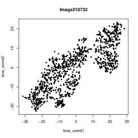
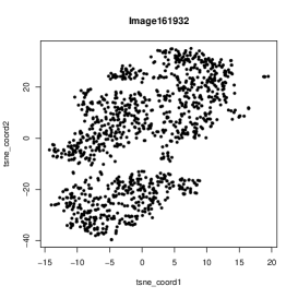
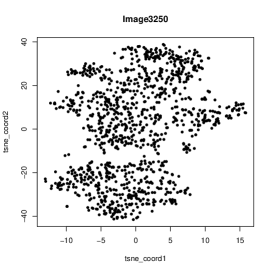
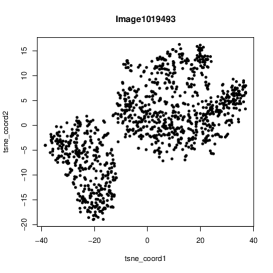
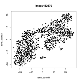
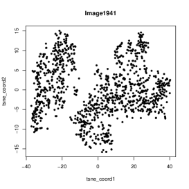
Figure 1: tSNE plots of cells in six randomly selected images/samples based on the expression levels of 30 epitopes or protein markers.

We focus on analyzing the conditional dependence network among these 30 protein epitopes and markers based on the single cell data for each of the samples or images. It is well known that the conditional dependence network can be modeled by Gaussian graphical model, which can be obtained using node-wise regression (Meinshausen and Bühlmann 2006; Yuan and Lin 2007). In other words, to obtain the dependence between two variables $X$ and $Y$ conditioning on all the other variables $(Z_{1},...,Z_{d})$, it suffices to perform a linear regression between $(X,Z_{1},...,Z_{d})$ against $Y$ and assess the coefficient of $X$. The construction of the conditional dependence network thus requires fitting such linear regressions over all the possible variable configurations. However, in our image cytometry data, heterogeneity among different cell-types may induce a mixture of different dependence structures. To address such an issue, we apply our proposed methods based on the sparse mixed linear regression model instead of the ordinary sparse linear regression model for network construction.

As an example, we first focus on the Image 210732. In addition to the global heterogeneity, we also observed that the marginal associations between many pairs of epitopes or markers contain a two-class mixture pattern, as shown in Figure 2. To obtain a conditional dependence network based on the 1,151 cells in this image, we fitted node-wise mixed linear regressions and for each of them performed the proposed multiple testing procedure with FDR $<10\%$. The final network (Figure, 3, top left) was constructed such that the edges indicate the identified associations from at least one of such node-wise regressions. To better illustrate the effects of mixture, the widths of the edges were set to be proportional to the $\ell_{2}$ distances between the two mixed regression coefficients, so that a thicker edge indicates a larger discrepancy between the two mixtures. As a comparison, we also obtained a network (Figure 3, top right) based on the standard node-wise Lasso and the multiple testing procedure of Javanmard and Javadi (2019) with the same FDR level. Similar to our simulation results, the standard Lasso-based methods tend to report many more associations than our proposed method, due to its failure to account for the underlying mixtures and the resulting underestimated $p$-values for the individual tests. In particular, we found that many heterogeneous associations shown by scatter plots in Figure 2 were indeed captured by our methods as the thicker edges in the network estimated by our mixture model.

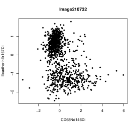
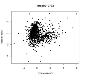
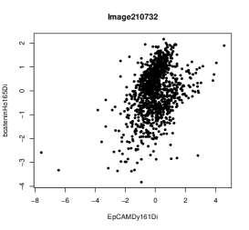
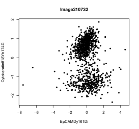
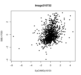
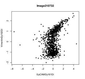
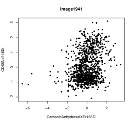
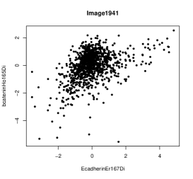
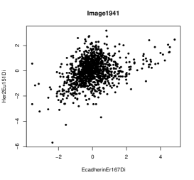
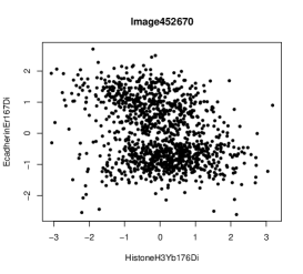
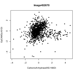
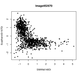
Figure 2: Pairwise scatter plots of epitope expressions for cells on different images, showing mixture of associations.

Naturally, the above analysis can be conducted similarly for each of the images. Here we present the results for Image 1941 and Image 452670, as two additional examples. With the global heterogeneity shown in Figure 1, again we obtained much denser networks from the standard Lasso based method and sparser networks from our proposed method (both with FDR $<10\%$ for the node-wise regressions). Moreover, many marginal associations (Figure 2) with heterogeneous associations had thicker edges of the networks based on our proposed method. Our analysis also suggests that the naive application of Lasso to heterogeneous datasets can lead to false associations.

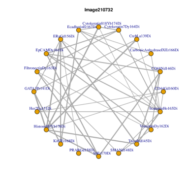
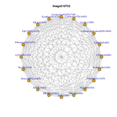
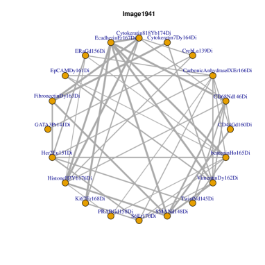
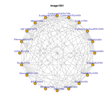
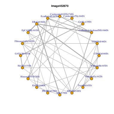
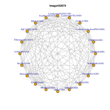
Figure 3: Networks of conditional dependence generated from node-wise regressions based on our proposed methods (left) and the standard Lasso based methods (right), both with FDR$<10\%$ for three different images. In the networks based on MLR, the widths of the edges were set to be proportional to the $\ell_{2}$ distances between the two mixed regression coefficients.

7 DISCUSSION

The present paper introduced an iterative estimation procedure using an EM algorithm, a debiased approach for individual coefficient inference based on the EM solutions, and a multiple testing procedure based on the debiased estimators for the high-dimensional mixed linear regression. Similar to many other works on EM algorithms (Balakrishnan et al. 2017; Yi et al. 2014; Wang et al. 2015; Yi and Caramanis 2015), sample splitting was used to facilitate the theoretical analysis in order to derive the estimation consistency. However, the numerical results suggest that such data splitting seems to be unnecessary for achieving the desirable results in practice. It is interesting to develop novel technical tools for analyzing the algorithms without splitting the sample.

The proposed EM algorithm assumes that the noise variance is known. Such an algorithm can be naturally extended to the case where the two noise variances are different and known. A more interesting problem is to develop an algorithm for the case where the two noise variances are different and unknown. In addition, this paper focuses on the two-class mixed regression model. It is interesting to extend the proposed algorithms to the general $k$-class mixed regression models and analyze its performance, especially when $k$ is unknown.

In addition to the estimation, individual coefficient inference and multiple testing problems considered in the current paper, there are several other interesting and related problems that are worth investigating. One such related problem is testing a single regression model against a mixed regression model. This involves, for example, the construction and analysis of a goodness-of-fit test. Finally, a natural generalization of the mixed linear regression model is the mixed generalized linear models (MGLM), where the outcome variables are allowed to be categorical. Estimation and multiple testing for high-dimensional MGLM are important and challenging problems that we leave for future research.

8 PROOFS

We present in this section the proofs of Theorems 2 and 5, the results on the individual coordinate inference and multiple testing. Theorem 3 can be proved by using the same derivation as that in Theorem 2, and the proofs Theorem 1 and other technical lemmas are given in the Supplementary Materials (Zhang et al. 2020).

8.1 Proof of Theorem 2

We first state the following lemmas.

Lemma 2.

Under the same conditions as in Theorem 1. For any given vector $\bm{m}^{*}\in\mathbb{R}^{p}$, there exists a constant $C>0$ such that

$$\|\mathbb{E}[\frac{1}{n_{T}}\sum_{i=1}^{n_{T}}\gamma_{\bm{\theta},i}^{(T)}\bm{x}_{i}\bm{x}_{i}^{\top}\bm{m}^{*}]-\mathbb{E}[\frac{1}{n_{T}}\sum_{i=1}^{n_{T}}\gamma_{\bm{\theta}^{*},i}\bm{x}_{i}\bm{x}_{i}^{\top}\bm{m}^{*}]\|_{2}\leq C\|\bm{m}^{*}\|_{2}\|\bm{\theta}^{*}-\hat{\bm{\theta}}^{(T)}\|_{2};$$

$$\|\mathbb{E}[\frac{1}{n_{T}}\sum_{i=1}^{n_{T}}\gamma_{\bm{\theta},i}^{(T)}\bm{x}_{i}\bm{x}_{i}^{\top}\bm{m}^{*}]-\frac{1}{n_{T}}\sum_{i=1}^{n_{T}}\gamma_{\bm{\theta},i}^{(T)}\bm{x}_{i}\bm{x}_{i}^{\top}\bm{m}^{*}\|_{\infty}=\|\bm{m}^{*}\|_{2}\cdot O_{p}(\sqrt{\frac{\log p}{n_{T}}}).$$

Lemma 3.

Under the same conditions as in Theorem 2. There exists a constant $c>0$ such that

$$\bm{m}_{j}^{\top}(T_{n}(\hat{\bm{\theta}}^{(T)}))_{1,1}\bm{m}_{j}\geq c,j\in[p].$$

Given the lemmas, we now proceed to proving Theorem 2. By symmetry, in the following, we only consider the case where $l=1$.

Recall that $n_{T}=n/T$ with $T\asymp\log n$, $\tilde{\Sigma}_{XX}=\frac{1}{n_{T}}\sum_{i=1}^{n_{T}}\bm{x}_{i}\bm{x}_{i}^{\top}$. We first verify that for $\mu=C\sqrt{\frac{\log p\log n}{n}}$ with sufficiently large constant $C$, the optimization of $\bm{m}_{j}$ is feasible, that is, there exits $\bm{m}_{j}^{*}\in\mathbb{R}^{p}$, such that $||\tilde{\Sigma}_{XX}\bm{m}_{j}^{*}-\bm{e}^{(p)}_{j}||_{\infty}\leq\mu$ and $\|\bm{m}_{j}^{*}\|_{1}\leq C\sqrt{\log n}$.

Take $\bm{m}_{j}^{*}=(\mathbb{\Sigma}^{-1})_{j}$ and use the fact that $\|\mathbb{\Sigma}^{-1}\|\leq L$, we have some $\|\bm{m}_{j}^{*}\|_{1}\leq C\sqrt{\log n}$.

Further, since $\|\bm{m}_{j}^{*}\|_{2}\leq C\sqrt{\log n}$ and $n/T\asymp n/\log n$, by the Bernstein inequality and union bound, we get

$$\|\mathbb{E}[\frac{1}{n_{T}}\sum_{i=1}^{n_{T}}\bm{x}_{i}\bm{x}_{i}^{\top}\bm{m}_{j}^{*}]-\frac{1}{n_{T}}\sum_{i=1}^{n_{T}}\bm{x}_{i}\bm{x}_{i}^{\top}\bm{m}_{j}^{*}\|_{\infty}=O_{p}(\sqrt{\frac{\log p}{n}}{\log n}).$$

Therefore, the optimization is feasible, and recall that the solution is denoted as $\tilde{\bm{m}}_{j}$. Then we proceed to showing the asymptotic normality.

For a given $j$, by (3.2), we have

$$\sqrt{n_{T}}(\widehat{\bm{\beta}}_{1j}^{u}-\bm{\beta}_{1j}^{*})= \sqrt{n_{T}}(\bm{m}_{j}^{\top}\widehat{\Sigma}_{XY}-\bm{m}_{j}^{\top}\widehat{\Sigma}_{XX}{\bm{\beta}_{1}^{*}})+\sqrt{n_{T}}(\bm{e}_{j}^{\top}-\bm{m}_{j}^{\top}\widehat{\Sigma}_{XX})(\hat{\bm{\beta}}_{1}^{(T)}-{\bm{\beta}}_{1}^{*})$$ (8.1)

$$= \sqrt{n_{T}}\bigg{[}\frac{1}{n_{T}}\sum_{i=1}^{n}\gamma_{\bm{\theta},i}^{(T)}(y_{i}-\langle\bm{x}_{i},\bm{\beta}_{1}^{*}\rangle)\bm{m}_{j}^{\top}\bm{x}_{i}\bigg{]}+\sqrt{n_{T}}\|\bm{e}_{j}^{\top}-\bm{m}_{j}^{\top}\widehat{\Sigma}_{XX}\|_{\infty}\cdot\|\hat{\bm{\beta}}_{1}^{(T)}-{\bm{\beta}}_{1}^{*}\|_{1}.$$

We then show that for $\bm{m}_{j}=\tilde{\bm{m}}_{j}/\hat{\omega}^{(T)}$, $\|\bm{e}_{j}^{\top}-\bm{m}_{j}^{\top}\widehat{\Sigma}_{XX}\|_{\infty}$ is small.

Recall that $\widehat{\Sigma}_{XX}=\frac{1}{n_{T}}\sum_{i=1}^{n_{T}}\gamma_{\bm{\theta},i}^{(T)}\bm{x}_{i}\bm{x}_{i}^{\top}$. By Lemma 2, we get

$$\|\mathbb{E}[\frac{1}{n_{T}}\sum_{i=1}^{n_{T}}\gamma_{\bm{\theta},i}^{(T)}\bm{x}_{i}\bm{x}_{i}^{\top}\bm{m}_{j}]-\mathbb{E}[\frac{1}{n_{T}}\sum_{i=1}^{n_{T}}\gamma_{\bm{\theta}^{*},i}\bm{x}_{i}\bm{x}_{i}^{\top}\bm{m}_{j}]\|_{2}\lesssim\|\bm{m}_{j}\|_{2}\cdot\|\bm{\theta}^{*}-\hat{\bm{\theta}}^{(T)}\|_{2}=O_{p}(\sqrt{\frac{s\log p}{n}}\log n),$$

and

$$\|\mathbb{E}[\frac{1}{n_{T}}\sum_{i=1}^{n_{T}}\gamma_{\bm{\theta},i}^{(T)}\bm{x}_{i}\bm{x}_{i}^{\top}\bm{m}_{j}^{*}]-\frac{1}{n_{T}}\sum_{i=1}^{n_{T}}\gamma_{\bm{\theta},i}^{(T)}\bm{x}_{i}\bm{x}_{i}^{\top}\bm{m}_{j}^{*}\|_{\infty}=O_{p}(\sqrt{\frac{\log p}{n}}\log n).$$

Let $z_{i}$ be the class for the pair of data $(\bm{x}_{i},y_{i})$, we obtain

$$\mathbb{E}[\frac{1}{n_{T}}\sum_{i=1}^{n_{T}}\gamma_{\bm{\theta}^{*},i}\bm{x}_{i}\bm{x}_{i}^{\top}\bm{m}_{j}^{*}]=\mathbb{E}[\frac{1}{n_{T}}\sum_{i=1}^{n_{T}}\mathbb{E}_{\hat{\bm{\theta}}^{*}}[1(z_{i}=1)\bm{x}_{i}\bm{x}_{i}^{\top}\bm{m}_{j}^{*}\mid\bm{x}_{i},y_{i}]]=\omega^{*}\bm{\Sigma}.$$

Therefore, we have

$$||\hat{\Sigma}_{XX}\bm{m}_{j}-\bm{e}^{(p)}_{j}||_{\infty}$$

$$= ||\mathbb{E}[\frac{1}{n_{T}}\sum_{i=1}^{n_{T}}\gamma_{\bm{\theta},i}^{(T)}\bm{x}_{i}\bm{x}_{i}^{\top}\bm{m}_{j}]-\frac{1}{n_{T}}\sum_{i=1}^{n_{T}}\gamma_{\bm{\theta},i}^{(T)}\bm{x}_{i}\bm{x}_{i}^{\top}\bm{m}_{j}||_{\infty}$$

$$+||\mathbb{E}[\frac{1}{n_{T}}\sum_{i=1}^{n_{T}}\gamma_{\bm{\theta},i}^{(T)}\bm{x}_{i}\bm{x}_{i}^{\top}\bm{m}_{j}]-\mathbb{E}[\frac{1}{n_{T}}\sum_{i=1}^{n_{T}}\gamma_{\bm{\theta}^{*},i}\bm{x}_{i}\bm{x}_{i}^{\top}\bm{m}_{j}]||_{\infty}+||\mathbb{E}[\frac{1}{n_{T}}\sum_{i=1}^{n}\gamma_{\bm{\theta}^{*},i}\bm{x}_{i}\bm{x}_{i}^{\top}\bm{m}_{j}]-\bm{e}^{(p)}_{j}||_{\infty}$$

$$= O_{p}(\sqrt{\frac{\log p}{n}}\log n)+O_{p}(\sqrt{\frac{s\log p}{n}}\log n)+\|\omega^{*}\mathbb{\Sigma}\bm{m}_{j}-\bm{e}_{j}^{(p)}\|_{\infty}$$

$$\leq O_{p}(\sqrt{\frac{s\log p}{n}}\log n)+\|\omega^{*}\mathbb{\Sigma}\bm{m}_{j}-\hat{\omega}^{(T)}\tilde{\Sigma}_{XX}\bm{m}_{j}\|_{\infty}+\|\hat{\omega}^{(T)}\tilde{\Sigma}_{XX}\bm{m}_{j}-\bm{e}_{j}^{(p)}\|_{\infty}$$

$$\leq O_{p}(\sqrt{\frac{s\log p}{n}}\log n)+\|\omega^{*}\mathbb{\Sigma}-\hat{\omega}^{(T)}\tilde{\Sigma}_{XX}\|_{\infty}\cdot\|\bm{m}_{j}\|_{1}+\|\tilde{\Sigma}_{XX}\tilde{\bm{m}}_{j}-\bm{e}_{j}^{(p)}\|_{\infty}$$

$$\leq O_{p}(\sqrt{\frac{s\log p}{n}}\log n).$$

Then (8.1) becomes

$$\sqrt{n_{T}}(\widehat{\bm{\beta}}_{1j}^{u}-\bm{\beta}_{1j}^{*})$$

$$= \sqrt{n_{T}}\bigg{[}\frac{1}{n_{T}}\sum_{i=1}^{n}\gamma_{\bm{\theta},i}^{(T)}(y_{i}-\langle\bm{x}_{i},\bm{\beta}_{1}^{*}\rangle)\bm{m}_{j}^{\top}\bm{x}_{i}\bigg{]}+\sqrt{n_{T}}\|\bm{e}_{j}^{\top}-\bm{m}_{j}^{\top}\widehat{\Sigma}_{XX}\|_{\infty}\cdot\|\hat{\bm{\beta}}_{1}^{(T)}-{\bm{\beta}}_{1}^{*}\|_{1}$$ (8.2)

$$= \langle\bm{m}_{j},\frac{1}{\sqrt{n_{T}}}\sum_{i=1}^{n_{T}}\gamma_{\bm{\theta},i}^{(T)}(y_{i}-\langle\bm{x}_{i},\bm{\beta}_{1}^{*}\rangle)\bm{x}_{i}\rangle+O_{P}(\frac{s^{3/2}\log p\log n}{\sqrt{n}})$$

$$= \langle\bm{m}_{j},\frac{1}{\sqrt{n_{T}}}\sum_{i=1}^{n_{T}}\gamma_{\bm{\theta},i}^{(T)}(y_{i}-\langle\bm{x}_{i},\bm{\beta}_{1}^{*}\rangle)\bm{x}_{i}\rangle+o_{P}(1).$$

Then, by Lemma 3, we have

$$\frac{\sqrt{n_{T}}\left(\widehat{\bm{\beta}}_{1j}^{u}-\bm{\beta}_{1j}^{*}\right)}{\sqrt{\hat{v}_{1j}}}=\frac{\langle\bm{m}_{j},\frac{1}{\sqrt{n}}\sum_{i=1}^{n}\gamma_{\bm{\theta},i}^{(T)}(y_{i}-\langle\bm{x}_{i},\bm{\beta}_{1}^{*}\rangle)\bm{x}_{i}\rangle}{\sqrt{\hat{v}_{1j}}}+o_{P}(1).$$

Finally, using Lemma 1, we obtain the desired result.

$$\frac{\sqrt{n}\left(\widehat{\bm{\beta}}_{1j}^{u}-\bm{\beta}_{1j}^{*}\right)}{\sqrt{\hat{v}_{1j}}}\stackrel{{\scriptstyle d}}{{\to}}N(0,1).$$

8.2 Proof of Theorem 5

We first consider the case when $\hat{t}$, given by (4.3), does not exist. In this case, we have $\hat{t}=\sqrt{2\log p}$. Note that for $j\in\mathcal{H}_{0}$, we have

$$T_{j}^{(1)}=\frac{\sqrt{n}\hat{\bm{\beta}}_{1,j}^{u}}{\hat{v}^{(1)}_{j}}=\frac{\langle\bm{m}_{j},\frac{1}{\sqrt{n}}\sum_{i=1}^{n}\gamma_{\bm{\theta}^{*},i}(y_{i}-\langle\bm{x}_{i},\bm{\beta}_{1}^{*}\rangle)\bm{x}_{i}\rangle}{\hat{v}^{(1)}_{j}}+\frac{\sqrt{n}Rem_{1}}{\hat{v}^{(1)}_{j}},$$

where $Rem_{1}=o_{P}(1/\sqrt{n})$, and a similar expression holds for $T_{j}^{(2)}$. Then we have

$$\mathbb{P}\bigg{(}\sum_{j\in\mathcal{H}_{0}}I\big{(}|T_{j}|\geq\sqrt{2\log p}\big{)}\geq 1\bigg{)}$$

$$\leq\mathbb{P}\bigg{(}\sum_{j\in\mathcal{H}_{0}}I\big{(}|T_{j}^{(1)}|\geq\sqrt{2\log p}\big{)}\geq 1\bigg{)}+\mathbb{P}\bigg{(}\sum_{j\in\mathcal{H}_{0}}I\big{(}|T_{j}^{(2)}|\geq\sqrt{2\log p}\big{)}\geq 1\bigg{)}$$

$$\leq\mathbb{P}\bigg{(}\sum_{j\in\mathcal{H}_{0}}I\bigg{(}\frac{\langle\bm{m}_{j},\frac{1}{\sqrt{n}}\sum_{i=1}^{n}\gamma_{\bm{\theta}^{*},i}(y_{i}-\langle\bm{x}_{i},\bm{\beta}_{1}^{*}\rangle)\bm{x}_{i}\rangle}{\hat{v}^{(1)}_{j}}+\frac{\sqrt{n}Rem_{1}}{\hat{v}^{(1)}_{j}}\geq\sqrt{2\log p}\bigg{)}\geq 1\bigg{)}$$

$$\quad+\mathbb{P}\bigg{(}\sum_{j\in\mathcal{H}_{0}}I\bigg{(}\frac{\langle\bm{m}_{j},\frac{1}{\sqrt{n}}\sum_{i=1}^{n}\gamma_{\bm{\theta}^{*},i}(y_{i}-\langle\bm{x}_{i},\bm{\beta}_{1}^{*}\rangle)\bm{x}_{i}\rangle}{\hat{v}^{(1)}_{j}}+\frac{\sqrt{n}Rem_{1}}{\hat{v}^{(1)}_{j}}\leq-\sqrt{2\log p}\bigg{)}\geq 1\bigg{)}$$

$$\quad+\mathbb{P}\bigg{(}\sum_{j\in\mathcal{H}_{0}}I\bigg{(}\frac{\langle\bm{m}_{j},\frac{1}{\sqrt{n}}\sum_{i=1}^{n}(1-\gamma_{\bm{\theta}^{*},i})(y_{i}-\langle\bm{x}_{i},\bm{\beta}_{2}^{*}\rangle)\bm{x}_{i}\rangle}{\hat{v}^{(2)}_{j}}+\frac{\sqrt{n}Rem_{2}}{\hat{v}^{(2)}_{j}}\geq\sqrt{2\log p}\bigg{)}\geq 1\bigg{)}$$

$$\quad+\mathbb{P}\bigg{(}\sum_{j\in\mathcal{H}_{0}}I\bigg{(}\frac{\langle\bm{m}_{j},\frac{1}{\sqrt{n}}\sum_{i=1}^{n}(1-\gamma_{\bm{\theta}^{*},i})(y_{i}-\langle\bm{x}_{i},\bm{\beta}_{2}^{*}\rangle)\bm{x}_{i}\rangle}{\hat{v}^{(2)}_{j}}+\frac{\sqrt{n}Rem_{2}}{\hat{v}^{(2)}_{j}}\leq-\sqrt{2\log p}\bigg{)}\geq 1\bigg{)}.$$ (8.3)

Define $(v^{(1)}_{j})^{2}={\rm Var}(\langle\bm{m}_{j},\frac{1}{\sqrt{n}}\sum_{i=1}^{n}\gamma_{\bm{\theta}^{*},i}(y_{i}-\langle\bm{x}_{i},\bm{\beta}_{1}^{*}\rangle)\bm{x}_{i}\rangle)$. For any $\epsilon>0$, we can bound the first term by

$$\mathbb{P}\bigg{(}\sum_{j\in\mathcal{H}_{0}}I\bigg{(}\frac{\langle\bm{m}_{j},\frac{1}{\sqrt{n}}\sum_{i=1}^{n}\gamma_{\bm{\theta}^{*},i}(y_{i}-\langle\bm{x}_{i},\bm{\beta}_{1}^{*}\rangle)\bm{x}_{i}\rangle}{\hat{v}^{(1)}_{j}}+\frac{\sqrt{n}Rem_{1}}{\hat{v}^{(1)}_{j}}\geq\sqrt{2\log p}\bigg{)}\geq 1\bigg{)}$$

$$=\mathbb{P}\bigg{(}\sum_{j\in\mathcal{H}_{0}}I\bigg{(}\frac{\langle\bm{m}_{j},\frac{1}{\sqrt{n}}\sum_{i=1}^{n}\gamma_{\bm{\theta}^{*},i}(y_{i}-\langle\bm{x}_{i},\bm{\beta}_{1}^{*}\rangle)\bm{x}_{i}\rangle}{{v}^{(1)}_{j}}\geq\frac{\hat{v}^{(1)}_{j}}{v^{(1)}_{j}}\sqrt{2\log p}-\frac{\sqrt{n}Rem_{1}}{{v}^{(1)}_{j}}\bigg{)}\geq 1\bigg{)}$$

$$\leq\mathbb{P}\bigg{(}\sum_{j\in\mathcal{H}_{0}}I\bigg{(}\frac{\langle\bm{m}_{j},\frac{1}{\sqrt{n}}\sum_{i=1}^{n}\gamma_{\bm{\theta}^{*},i}(y_{i}-\langle\bm{x}_{i},\bm{\beta}_{1}^{*}\rangle)\bm{x}_{i}\rangle}{{v}^{(1)}_{j}}\geq(1-\epsilon)\sqrt{2\log p}-\epsilon\bigg{)}\geq 1\bigg{)}$$

$$\quad+\mathbb{P}\bigg{(}\max_{j\in\mathcal{H}_{0}}\bigg{|}\frac{\sqrt{n}Rem_{1}}{{v}^{(1)}_{j}}\bigg{|}\geq\epsilon\bigg{)}+\mathbb{P}\bigg{(}\bigg{|}\frac{\hat{v}^{(1)}_{j}}{v^{(1)}_{j}}-1\bigg{|}\geq\epsilon\bigg{)}$$

$$\leq p\max_{j\in\mathcal{H}_{0}}\mathbb{P}\bigg{(}\frac{\langle\bm{m}_{j},\frac{1}{\sqrt{n}}\sum_{i=1}^{n}\gamma_{\bm{\theta}^{*},i}(y_{i}-\langle\bm{x}_{i},\bm{\beta}_{1}^{*}\rangle)\bm{x}_{i}\rangle}{{v}^{(1)}_{j}}\geq(1-\epsilon)\sqrt{2\log p}-\epsilon\bigg{)}+\mathbb{P}\bigg{(}\max_{j\in\mathcal{H}_{0}}\bigg{|}\frac{\sqrt{n}Rem_{1}}{{v}^{(1)}_{j}}\bigg{|}\geq\epsilon\bigg{)}$$

$$\quad+\mathbb{P}\bigg{(}\bigg{|}\frac{\hat{v}^{(1)}_{j}}{v^{(1)}_{j}}-1\bigg{|}\geq\epsilon\bigg{)}.$$

By the proof of Theorem 2, we know that

$$\mathbb{P}\bigg{(}\max_{j\in\mathcal{H}_{0}}\bigg{|}\frac{\sqrt{n}Rem_{1}}{v^{(1)}_{j}}\bigg{|}\geq\epsilon\bigg{)}\to 0,\qquad\mathbb{P}\bigg{(}\bigg{|}\frac{\hat{v}^{(1)}_{j}}{v^{(1)}_{j}}-1\bigg{|}\geq\epsilon\bigg{)}\to 0.$$

In addition, for $j\in\mathcal{H}_{0}$, let

$$T_{0j}^{(1)}=\frac{\langle\bm{m}_{j},\frac{1}{\sqrt{n}}\sum_{i=1}^{n}\gamma_{\bm{\theta}^{*},i}(y_{i}-\langle\bm{x}_{i},\bm{\beta}_{1}^{*}\rangle)\bm{x}_{i}\rangle}{{v}^{(1)}_{j}}.$$

where $\mathbb{E}\langle\bm{m}_{j},\gamma_{\bm{\theta}^{*},i}(y_{i}-\langle\bm{x}_{i},\bm{\beta}_{1}^{*}\rangle)\bm{x}_{i}\rangle/v^{(1)}_{j}=0$ and $\text{Var}(\mathbb{E}\langle\bm{m}_{j},\gamma_{\bm{\theta}^{*},i}(y_{i}-\langle\bm{x}_{i},\bm{\beta}_{1}^{*}\rangle)\bm{x}_{i}\rangle/v^{(1)}_{j})=1$. Conditional on $X$ by Lemma 6.1 of Liu (2013), we have

$$\sup_{0\leq t\leq 4\sqrt{\log p}}\bigg{|}\frac{P(|T_{0j}^{(1)}|\geq t)}{G(t)}-1\bigg{|}\leq C(\log p)^{-1}.$$ (8.4)

Hereafter, unless explicitly noted, all of our discussion will be conditional on $\{\bm{x}_{i}\}_{i=1}^{n}$. Now let $t=(1-\epsilon)\sqrt{2\log p}-2\epsilon$, we have

$$\mathbb{P}\bigg{(}T_{0j}^{(1)}\geq(1-\epsilon)\sqrt{2\log p}-2\epsilon\bigg{)}\leq G((1-\epsilon)\sqrt{2\log p}-2\epsilon)+C\frac{G((1-\epsilon)\sqrt{2\log p}-2\epsilon)}{\log p}.$$

Hence

$$p\max_{j\in\mathcal{H}_{0}}\mathbb{P}\bigg{(}T_{0j}\geq(1-\epsilon)\sqrt{2\log p}-\epsilon\bigg{)}\leq CpG((1-\epsilon)\sqrt{2\log p}-2\epsilon)+O(p^{-c}),$$

which goes to zero as $(n,p)\to\infty$. By symmetry, we know that the rest three terms in (8.2) also goes to 0. Therefore we have proved the theorem when $\hat{t}=\sqrt{2\log p}$.

Now consider the case when $0\leq\hat{t}\leq b_{p}$ holds. We have

$$\text{FDP}(\hat{t}) =\frac{\sum_{j\in\mathcal{H}_{0}}I\{|T_{j}|\geq\hat{t}\}}{\max\big{\{}\sum_{j=1}^{p}I\{|T_{j}|\geq\hat{t}\},1\big{\}}}\leq\frac{\sum_{j\in\mathcal{H}_{0}}I\{|T_{j}^{(1)}|\geq\hat{t}\}+\sum_{j\in\mathcal{H}_{0}}I\{|T_{j}^{(2)}|\geq\hat{t}\}}{\max\big{\{}\sum_{j=1}^{p}I\{|T_{j}|\geq\hat{t}\},1\big{\}}}.$$

Note that for $\ell=1,2$,

$$\frac{\sum_{j\in\mathcal{H}_{0}}I\{|T_{j}^{(\ell)}|\geq\hat{t}\}}{\max\big{\{}\sum_{j=1}^{p}I\{|T_{j}|\geq\hat{t}\},1\big{\}}}\leq\frac{p_{0}G(\hat{t})}{\max\big{\{}\sum_{j=1}^{p}I\{|T_{j}|\geq\hat{t}\},1\big{\}}}(1+A^{(\ell)}_{p})$$

where

$$A_{p}^{(\ell)}=\sup_{0\leq t\leq b_{p}}\bigg{|}\frac{\sum_{j\in\mathcal{H}_{0}}I\{|T_{j}^{(\ell)}|\geq t\}}{p_{0}G(t)}-1\bigg{|}.$$

Note that by definition

$$\frac{p_{0}G(\hat{t})}{\max\big{\{}\sum_{j=1}^{p}I\{|T_{j}|\geq\hat{t}\},1\big{\}}}\leq\frac{p_{0}\alpha}{p}.$$

The proof is complete if $A_{p}^{(\ell)}\to 0$ in probability. The rest of the proof is devoted to it. We first show that

$$|T_{j}^{(\ell)}-T_{0j}^{(\ell)}|=o_{P}(1/\sqrt{\log p}).$$ (8.5)

To see this, we notice that, under the sparsity condition $s=o\big{(}\frac{n^{1/2}}{\log^{3/2}p\log n}\big{)}$, with probability at least $1-O(p^{-c})$,

$$|T_{j}^{(\ell)}-T_{0j}^{(\ell)}| \leq\bigg{|}\frac{\sqrt{n}Rem_{\ell}}{{v}^{(\ell)}_{j}}\bigg{|}\cdot\bigg{|}\frac{v_{j}^{(\ell)}}{\hat{v}^{(\ell)}_{j}}\bigg{|}+\bigg{|}T^{(\ell)}_{0j}({v}^{(\ell)}_{j}/\hat{v}^{(\ell)}_{j}-1)\bigg{|}=o\bigg{(}\frac{1}{\sqrt{\log p}}\bigg{)}.$$

By the fact that $G(t+o(1/\sqrt{\log p}))/G(t)=1+o(1)$ uniformly in $0\leq t\leq\sqrt{2\log p}$, it suffices to show that

$$\sup_{0\leq t\leq b_{p}}\bigg{|}\frac{\sum_{j\in\mathcal{H}_{0}}I\{|T_{0j}^{(\ell)}|\geq t\}}{p_{0}G(t)}-1\bigg{|}\rightarrow 0\quad\text{ in probability.}$$ (8.6)

Let $z_{0}<z_{1}<...<z_{d_{p}}\leq 1$ and $t_{i}=G^{-1}(z_{i})$, where $z_{0}=G(b_{p})$, $z_{i}=c_{p}/p+c_{p}^{2/3}e^{i^{\delta}}/p$ with $c_{p}=pG(b_{p})$, and $d_{p}=[\log((p-c_{p})/c_{p}^{2/3})]^{1/\delta}$ and $0<\delta<1$, which will be specified later. We have $G(t_{i})/G(t_{i+1})=1+o(1)$ uniformly in $i$, and $t_{0}/\sqrt{2\log(p/c_{p})}=1+o(1)$. Note that uniformly for $1\leq j\leq m$, $G(t_{i})/G(t_{i-1})\to 1$ as $p\to\infty$. The proof of (8.6) reduces to show that

$$\max_{0\leq i\leq d_{p}}\bigg{|}\frac{\sum_{j\in\mathcal{H}_{0}}I\{|T^{(\ell)}_{0j}|\geq t_{i}\}}{p_{0}G(t_{i})}-1\bigg{|}\rightarrow 0$$ (8.7)

in probability. Hereafter, we omit the dependence on the index $\ell$ for simplicity. In fact, for each $\epsilon>0$, we have

$$\mathbb{P}\bigg{(}\max_{0\leq i\leq d_{p}}\bigg{|}\frac{\sum_{j\in\mathcal{H}_{0}}[I\{|T_{0j}|\geq t_{i}\}-G(t_{i})]}{p_{0}G(t_{i})}\bigg{|}\geq\epsilon\bigg{)}\leq\sum_{j=0}^{d_{p}}\mathbb{P}\bigg{(}\bigg{|}\frac{\sum_{j\in\mathcal{H}_{0}}[I\{|T_{0j}|\geq t_{i}\}-G(t_{i})]}{p_{0}G(t_{i})}\bigg{|}\geq\epsilon/2\bigg{)}.$$

Set $I(t)=\frac{\sum_{j\in\mathcal{H}_{0}}[I\{|T_{0j}|\geq t\}-P(|T_{0j}|\geq t)]}{p_{0}G(t)}.$ By Markov’s inequality $P(|I(t_{i})|\geq\epsilon/2)\leq\frac{\mathbb{E}[I(t_{i})]^{2}}{\epsilon^{2}/4},$ and it suffices to show $\sum_{j=0}^{d_{p}}\mathbb{E}[I(t_{i})]^{2}=o(1)$. To see this, by (8.4),

$$\mathbb{E}I^{2}(t) =\frac{\sum_{j\in\mathcal{H}_{0}}[P(|T_{0j}|\geq t)-P^{2}(|T_{0j}|\geq t)]}{p_{0}^{2}G^{2}(t)}$$

$$\quad+\frac{\sum_{j,k\in\mathcal{H}_{0},k\neq j}[P(|T_{0k}|\geq t,|T_{0j}|\geq t)-P(|T_{0k}|\geq t)P(|T_{0j}|\geq t)]}{p_{0}^{2}G^{2}(t)}$$

$$\leq\frac{C}{p_{0}G(t)}+\frac{1}{p_{0}^{2}}\sum_{(j,k)\in\mathcal{A}(\epsilon)\cap\mathcal{H}_{0}}\frac{P(|T_{0k}|\geq t,|T_{0j}|\geq t)}{G^{2}(t)}$$

$$\quad+\frac{1}{p_{0}^{2}}\sum_{(j,k)\in\mathcal{A}(\epsilon)^{c}\cap\mathcal{H}_{0}}\bigg{[}\frac{P(|T_{0k}|\geq t,|T_{0j}|\geq t)}{G^{2}(t)}-1\bigg{]}$$

$$=\frac{C}{p_{0}G(t)}+I_{11}(t)+I_{12}(t).$$

For $(j,k)\in\mathcal{A}(\epsilon)^{c}\cap\mathcal{H}_{0}$, applying Lemma 6.1 in Liu (2013), we have $I_{12}(t)\leq C(\log p)^{-1-\xi}$ for some $\xi>0$ uniformly in $0<t<\sqrt{2\log p}$. By Lemma 6.2 in Liu (2013), for $(j,k)\in\mathcal{A}(\epsilon)\cap\mathcal{H}_{0}$, we have

$$P(|T_{0k}|\geq t,|T_{0j}|\geq t)\leq C(t+1)^{-2}\exp\bigg{(}-\frac{t^{2}}{1+|\rho_{jk}|}\bigg{)}.$$

So that

$$I_{11}(t)\leq C\frac{1}{p_{0}^{2}}\sum_{(j,k)\in\mathcal{A}(\epsilon)\cap\mathcal{H}_{0}}(t+1)^{-2}\exp\bigg{(}-\frac{t^{2}}{1+|\rho_{jk}|}\bigg{)}G^{-2}(t)\leq C\frac{1}{p_{0}^{2}}\sum_{(j,k)\in\mathcal{A}(\epsilon)\cap\mathcal{H}_{0}}[G(t)]^{-\frac{2|\rho_{jk}|}{1+|\rho_{jk}|}}.$$

Note that for $0\leq t\leq b_{p}$, we have $G(t)\geq G(b_{p})=c_{p}/p$, so that by assumption (A3) it follows that for some $\epsilon,q>0$,

$$I_{11}(t)\leq C\sum_{(j,k)\in\mathcal{A}(\epsilon)\cap\mathcal{H}_{0}}p^{\frac{2|\rho_{jk}|}{1+|\rho_{jk}|}+q-2}=O(1/(\log p)^{2}).$$

By the above inequalities, we can prove (8.7) by choosing $0<\delta<1$ so that

$$\sum_{i=0}^{d_{p}}\mathbb{E}[I(t_{i})]^{2} \leq C\sum_{i=0}^{d_{p}}(pG(t_{i}))^{-1}+Cd_{p}[(\log p)^{-1-\delta}+(\log p)^{-2}]$$

$$\leq C\sum_{i=0}^{d_{p}}\frac{1}{c_{p}+c_{p}^{2/3}e^{i^{\delta}}}+o(1)$$

$$=o(1).$$

Lately, as all the above arguments are conditional on $\{\bm{x}_{i}\}_{i=1}^{n}$, the statements of Theorem 5 follow by averaging over the probability measure of $\{\bm{x}_{i}\}_{i=1}^{n}$ . ∎

FUNDING

This research was supported by NIH grants R01GM123056 and R01GM129781 and NSF grant DMS-1712735.

SUPPLEMENTARY MATERIALS

In the Supplemental Materials, we prove all the main theorems and the technical lemmas.