Perfect state transfer on hypercubes and its implementation using superconducting qubits

Abstract

We propose a protocol for perfect state transfer between any pair of vertices in a hypercube. Given a pair of distinct vertices in the hypercube we determine a sub-hypercube that contains the pair of vertices as antipodal vertices. Then a switching process is introduced for determining the sub-hypercube of a memory enhanced hypercube that facilitates perfect state transfer between the desired pair of vertices. Furthermore, we propose a physical architecture for the pretty good state transfer implementation of our switching protocol with fidelity arbitrary close to unity, using superconducting transmon qubits with tunable couplings. The switching is realised by the control over the effective coupling between the qubits resulting from the effect of ancilla qubit couplers for the graph edges. We also report an error bound on the fidelity of state transfer due to faulty implementation of our protocol.

I Introduction

In quantum computation, it is often required to transfer an arbitrary quantum state from one location to another ref:48 . Especially in large scale QIP, this is an important task, connecting two sites that may belong to the same or different quantum processors. The latter is nontrivial for many quantum information processing (QIP) realizations, such as, solid state quantum computing and superconducting quantum computing ref:77 ; ref:75 ; ref:71 ; ref:72 ; ref:73 ; ref:74 ; ref:23 . It is also very important to find the systems that support this quantum information exchange between distant sites to realize this phenomenon. For the short distance communication (such as adjacent quantum processors), methods for interfacing different kinds of physical systems are much required, for example, ion traps ref:39 ; ref:34 , superconducting circuits ref:41 ; ref:42 , boson lattices ref:76 , etc. The task of state transfer is incorporated with the idea of reducing the manipulation required to communicate between distant computational qubits in a large scale quantum computer ref:54 ; ref:49 . Scalability of quantum processors is a deep concern in the development of quantum computing hardware ref:26 ; ref:27 ; ref:28 . This is essential for determining how good is an architecture for quantum information processing ref:30 .

Quantum state transfer with 100% fidelity is known as perfect state transfer (PST) and this idea using interacting spin-1/2 particles was first proposed in ref:1 . This is established by utilizing a combinatorial graph structure as a platform for actual quantum network in the first excitation subspace of multi-qubit system ref:15 ; ref:2 . In general, this involves mixed states of the network qubits ref:57 , however, showing PST for pure states in a graph suffices to prove the phenomenon. PST can be used in entanglement transfer, quantum communication, signal amplification, quantum information recovery and implementation of universal quantum computation ref:18 ; ref:49 ; ref:60 ; ref:61 . It is important to find classes of graphs where PST is possible and equally important to find graphs where it does ref:58 ; ref:12 , in order to classify how good is an architecture for quantum information processing. The idea of pretty good state transfer is also studied, where the transfer fidelity is less than unity but occurring on a large number of graphs that support state transfer ref:66 ; ref:67 ; ref:68 ; ref:79 ; ref:83 and in general these graphs can be weighted ref:65 . More general graphs such as signed graphs ref:50 and oriented graphs ref:19 are also studied. PST for qudits has also been classified for some networks ref:53 ; ref:21 . One of the big challenges for scalable quantum architecture is the imperfect two-qubit interaction. For PST with maximum fidelity, the pairwise interaction should be improved for large-scale quantum processors ref:31 . Different physical systems for quantum computation have different advantages, such as, high-fidelity and control in ion-traps ref:35 ; ref:34 versus the scalability of superconducting circuits ref:33 ; ref:23 ; ref:32 . PST was demonstrated in the latter, with tunable qubit couplings ref:78 . Here, we propose a protocol for large scale quantum processors with support on hypercube network.

The scheme established in ref:4 and ref:5 allows PST over arbitrary long distances. Here the shortcoming is that the PST is possible only between antipodal vertices. A switching technique is proposed in ref:56 where in a complete graph $K_{n}$, switching off one link establishes PST in non-adjacent qubits. This enables PST for more vertices but still does not enable routing to different vertices and there is no scalability, the graph remains fixed. One attempt at switching and routing is proposed in ref:59 which involves creating new edges and coupling for qubits, however, is still not scalable. Various other works describe methods of routing of excitations in spin chains ref:80 ; ref:81 ; ref:82 , limited to one dimension. In this work, we resolve this problem through our hypercube switching scheme. The goal of this paper is three fold: $1)$ showing perfect state transfer is possible between any pair of vertices in an $n$-dimensional hypercube by introducing a concept of switching on and off of edges of the hypercube, $2)$ defining an effective Hamiltonian that can implement the sub-hypercube architecture with the proposed switching, $3)$ finding an error bound of the fidelity of the PST for an inaccurate implementation of the sub-hypercube in an experimental setup.

The rest of the paper is organized as follows. We recall some preliminary results in section II that are needed to establish our results. In section III, given a pair of distinct vertices in a $n$-dimensional hypercube ${\mathcal{Q}}_{n},$ a unique sub-hypercube ${\mathcal{Q}}_{d},d\leq n$ is determined such that the given pair of vertices are antipodal vertices of ${\mathcal{Q}}_{d}.$ We also describe how a memory enhanced hypercube enables to identify the vertices of the sub-hypercube. Consequently, the perfect state transfer is established between those pair of vertices. A proposal for the implementation of our switching protocol is presented in section IV using superconducting transmon qubits.

II Preliminaries

A graph is an ordered pair $G=(V,E)$, where $V$ denotes the set of vertices (or nodes), and $E\subseteq\{(u,v)\in V\times V|u\neq v\}$ denotes the set of edges, which are unordered pairs of vertices. Let $I\subseteq V.$ Then a subgraph of the graph $G$ defined by the vertex set $I$ is called an induced subgraph if two distinct vertices in $I$ are linked by an edge in the subgraph if and only if they are linked by an edge in $G$ west2001introduction . Obviously, induced subgraph defined by a set of vertices is unique.

Let $G$ be a graph with $n$ vertices with $n=|V|$ and $V=\{0,1,2,\ldots,n-1\}.$ Then the adjacency matrix $A(G)=[a_{ij}]$ associated with $G$ is defined as $a_{ij}=1$ if $(i,j)\in E$ and $0$ otherwise. Obviously, $A(G)$ is a symmetric matrix of order $n\times n.$ Then the degree of $i\in V$ is defined as $\mbox{deg}(i)=\sum_{j=0}^{n-1}a_{ij}.$ The degree matrix $D(G)=\mbox{diag}(d_{0},\ldots,d_{n-1})$ of $G$ is a diagonal matrix where $d_{i}=\mbox{deg}(i),0\leq i\leq n-1.$ The graph Laplacian matrix $L(G)$ associated with the graph $G$ is defined as $L(G)=D(G)-A(G).$ These two matrices encode the structure of the graph, and determine the architecture by determining qubits’ mutual couplings and connectivity.

PST of a state in a many-qubit system is formulated by a combinatorial graph in which the edges of the graph represents coupling of qubits. This is interpreted by beginning with a single-qubit state (generally mixed) $\rho_{\text{qubit}}^{u}$ at some site $u$, and $\rho_{\text{in}}$ taken as the state of the rest of the system, and after evolution for some finite time $t_{0}$, with an interaction Hamiltonian $H$, the final evolved state

$$e^{-iHt_{0}/\hbar}(\rho_{\text{qubit}}^{u}\otimes\rho_{\text{in}})e^{iHt_{0}/\hbar}=\rho_{\text{qubit}}^{v}\otimes\rho_{\text{out}}$$ (1)

is obtained, thereby transmitting the respective qubit state to another desired vertex $v$ of the graph. In general, $\rho_{\text{qubit}}$ is a density matrix, however, in this paper we consider that it corresponds to a pure state. The most simplified case for such realization is the one-dimensional chain of qubits.

There are two kinds of well known interaction Hamiltonian for the pairwise interactions defined by the edges between the qubits which are placed at the vertices of a graph. The first is the XY model in two spatial degrees of freedom,

$$\begin{split}\frac{H_{XY}}{\hbar}&=\sum_{(i,j)\in E(G)}J_{ij}\left(\sigma^{x}_{i}\sigma^{x}_{j}+\sigma^{y}_{i}\sigma^{y}_{j}\right)\\ &=\sum_{(i,j)\in E(G)}2J_{ij}\left(\sigma^{+}_{i}\sigma^{-}_{j}+\sigma^{-}_{i}\sigma^{+}_{j}\right),\end{split}$$ (2)

where $\sigma_{i}^{\pm}$ are the ladder operators acting on the qubit placed at vertex $i$ such that $\sigma^{\pm}_{i}=\sigma_{i}^{x}\pm i\sigma^{y}_{i}$, with $\sigma^{x,y}_{i}$ are the Pauli matrices. The second connection is via the three-dimensional Heisenberg model,

$$\frac{H_{Hei}}{\hbar}=-\sum_{(i,j)\in E(G)}J_{ij}\vec{\sigma}_{i}\cdot\vec{\sigma}_{j}+\sum_{j}B_{j}\sigma^{z}_{j}$$ (3)

where, $\vec{\sigma}_{i}$ is Pauli matrix vector $\vec{\sigma}_{i}=(\sigma^{x}_{i},\sigma^{y}_{i},\sigma^{z}_{i})$ for the $i$th spin and $I_{i}$ is the identity operator for the $i$th vertex.

In this paper, we consider the general many-body XY-coupling as well as the Heisenberg Hamiltonian and consider the coupling strength $J_{ij}$ to be a real parameter that can be continuously changed. In addition, we consider the local fields $B_{j}$ to tune the diagonal terms of the Hamiltonian such that it coincides with the Laplacian of the graph. This special choice is always possible ref:4 . We also emphasize that these two coupling Hamiltonian need not necessarily correspond to spin-1/2 particle interaction. In the first excitation subspace for the qubits, XY-coupling Hamiltonian and Heisenberg Hamiltonian action is equivalent to adjacency and Laplacian action respectively, for the corresponding graph, in the vertex space ref:15 . Initially, the system is in its ground state $|0\rangle=|000...0\rangle$, where the ket $|0\rangle$ denotes the single qubit ground state. We have the graph vertex-space states $|i\rangle=|00...010....0\rangle$ ($i=1,2,..,n$), in which the qubit at the $i$th site is in the first excited state $|1\rangle$. To start the PST procedure, $A$ encodes an unknown (and arbitrary) state $|\psi_{in}\rangle=\cos(\theta/2)|0\rangle+e^{i\phi}\sin(\theta/2)|1\rangle$ at site $A$ in the graph and lets the system evolve freely for a finite time $t=t_{0}$ at which, the quantum state localizes at another site $B$ in the many-body system. This free quantum evolution of the entire network is precisely the quantum walk on the corresponding graph $G$ corresponding to the many-body network.

To define quantum walk and state transfer on a graph $G=(V,E)$ of $n=|V|$ vertices, $n$-qubit states are considered that are localized at the vertices of the graph, equivalently the excitation space isomorphic to ${\mathbb{C}}^{|V|}.$ A continuous time quantum walk on a graph $G$ is the Schrödinger evolution of the graph composite state with the graph adjacency matrix $A(G)$ as the Hamiltonian kendon2011perfect . If $\ket{\zeta(0)}\in\mathbb{C}^{|V|}$ is the initial quantum state, then the evolution of the quantum walk is given by

$$\ket{\zeta(t)}=\exp(-itA(G))\ket{\zeta(0)},$$ (4)

The probability for getting the quantum state localised at the vertex $v$ at time $t$ is given by $|\braket{v}{\zeta(t)}|^{2}$. $G$ has a PST from vertex $u$ to vertex $v$ at finite time $t_{0}$ if

$$|\braket{v}{\exp(-it_{0}A(G))}{u}|=1.$$ (5)

This is the same condition for perfect state transfer expressed in graph theoretic fashion ref:7 and implies Eqn. (1). The graph $G$ allows a perfect state transfer from the vertex $u$ to $v$ if the $(u,v)$-th term of $\exp(-itA(G))$ has magnitude $1$. Similarly, Laplacian PST is when the $(u,v)$-th term of $\exp(-itL(G))$ has magnitude $1$

Some well-known examples of graphs which allow perfect state transfer over long distances are ref:4 ; ref:5 :

1. The complete graph $K_{2}$ with two vertices allow perfect state transfer between its vertices in time $t_{0}=\pi/2$ (in the units of energy inverse).

2. The path graph $P_{3}$ has perfect state transfer between its end vertices in time $t_{0}=\pi/\sqrt{2}$ (in the units of energy inverse).

3. The hypercube of any order has perfect state transfer between its antipodal points in the same time $\pi/2$. Besides, on any order of Cartesian product of $P_{3}$ has PST between its antipodal vertices in the same time $\pi/\sqrt{2}$.

Above three results hold both for the XY-coupling as well as the Heisenberg interaction. We make use of these results in order to establish a process for PST between any pair of vertices in hypercube of any dimension.

III Memory-enhanced perfect state transfer on hypercubes

A hypercube of dimension $n$, denoted by $\mathcal{Q}_{n}$ is a graph on $2^{n}$ vertices, $n\geq 0$ which can be defined as an $n$-times Cartesian product of the complete graph on $2$ vertices, which is an edge. Let the vertex set of the complete graph on two vertices be $\{0,1\}.$ Then the vertices of ${\mathcal{Q}}_{n}$ are labeled as the $n$-tuples of $0$ and $1$, that is, the vertex set of ${\mathcal{Q}}_{n}$ is $\mathcal{V}_{n}=\{0,1\}^{n}.$ Two vertices $x,y$ of ${\mathcal{Q}}_{n}$ are linked by an edge if the Hamming distance of $x,y\in\{0,1\}^{n}$ is one. Two vertices $x=(x_{1},\ldots,x_{n})$ and $y=(y_{1},\ldots,y_{n})$ of $Q_{n}$ are called antipodal if $x_{i}\neq y_{i},$ $i\in\{1,\ldots,n\}.$ Given two vertices $x$ and $y$, we are interested to determine the unique induced sub-hypercube ${\mathcal{Q}}_{d}$ for some $d$ of ${\mathcal{Q}}_{n},n\geq d$ such that the vertices $x,y$ of ${\mathcal{Q}}_{n}$ are antipodal in ${\mathcal{Q}}_{d}$. The following proposition describes the same.

Proposition III.1.

Let $x=(x_{1},\ldots,x_{n}),$ $y=(y_{1},\ldots,y_{n})\in\mathcal{V}_{n},$ the vertex set of ${\mathcal{Q}}_{n}.$ Suppose $d=|\{i:x_{i}\neq y_{i},i=1,\ldots,n\}|.$ Then the unique induced sub-hypercube ${\mathcal{Q}}_{d}$ of ${\mathcal{Q}}_{n}$ with $x,y$ as antipodal vertices of ${\mathcal{Q}}_{d}$ is given by the set of vertices

$$\begin{split}\mathcal{V}_{d}=&\{z=(z_{1},\ldots,z_{n})\in\mathcal{V}_{n}:z_{i}=x_{i},\,\,\mbox{if}\,x_{i}=y_{i},\,\mbox{and}\\ &z_{i}\in\{0,1\}\,\mbox{otherwise},i=1,\ldots,n\}.\end{split}$$ (6)

Proof. Note that if $d=n$ then $x,y$ are antipodal vertices of ${\mathcal{Q}}_{n}.$ Now let $n-d\neq 0.$ Then there are indices $i_{1},\ldots,i_{n-d}$ such that $x_{i_{j}}=y_{i_{j}},$ $j\in\{1,\ldots,n-d\}.$ Consider the set of vertices

$$\begin{split}\mathcal{V}_{d}=&\{z=(z_{1},\ldots,z_{n})\in\{0,1\}^{n}:z_{i_{j}}=x_{i_{j}}=y_{i_{j}},\\ &j=1,\ldots,n-d\}.\end{split}$$ (7)

Then $|\mathcal{V}_{d}|=2^{d}.$ Consider the subgraph of ${\mathcal{Q}}_{n}$ that is induced by the vertex set $\mathcal{V}_{d}.$ Thus $z,w\in\mathcal{V}_{d}$ are linked by edge in the induced subgraph if and only if $z,w$ are linked by an edge in ${\mathcal{Q}}_{n},$ that is, Hamming distance between $z$ and $w$ is $1.$ The uniqueness of the sub-hypercube ${\mathcal{Q}}_{d}$ of ${\mathcal{Q}}_{n}$ follows from the fact that it is an induced subgraph of ${\mathcal{Q}}_{n}$. This completes the proof. $\hfill{\square}$

Now we propose a procedure to utilize the induced $d$-dimensional sub-hypercubes of an $n$-dimensional hypercube ${\mathcal{Q}}_{n}$, $n\geq d$ for perfect transfer of qubits between any pair of nodes in ${\mathcal{Q}}_{n}.$

In the following we describe how a classical $n$-bit or $n$-qubit quantum memory address register corresponding to every vertex of ${\mathcal{Q}}_{n}$ can help to obtain the desired state transfer between a pair of arbitrary vertices of ${\mathcal{Q}}_{n}.$ As discussed above, each vertex of ${\mathcal{Q}}_{n}$ can be labeled as an element of $\{0,1\}^{n}.$ Let $x=(x_{1},\ldots,x_{n})\in\mathcal{V}_{n}=\{0,1\}^{n}.$ Then consider a classical $n$-bit memory which stores the labelling of a vertex or quantum memory register which store the corresponding $n$-qubit product state $\ket{x}$ for the vertex $x.$ For the classical memory design and architecture, it is a standard procedure that the digital information of the classical bit $0$ or $1$ can be stored by distinguishing between different values of some continuous physical quantity, such as voltage or current. Besides, many organizations are possible for a memory design based on the choices of the number of cells in a memory and each cell contains a fixed number of bits, see tanenbaum2016structured ; patterson2016computer . Setting $n$ bits of data in a cell, a memory of $n2^{n}$ bits of data is possible having $2^{n}$ memory addresses. In the present standard of architecture a large number of bits can be stored in a memory, for example, in semiconductor memory devices millions of bits can be stored and accessed tanenbaum2016structured . Each cell is labelled with a memory address and a desired collection of addresses can be accessed by a program efficiently gabbrielli2010programming . Hence the vertices with desired bits at the desired positions in the cells corresponding to all the vertices of the hypercube can be determined and the vertices of the sub-hypercube ${\mathcal{Q}}_{d}$ can be identified. On the other hand, observe that $\{\ket{x}:x\in\mathcal{V}_{n}\}$ is the canonical orthonormal basis of $({\mathbb{C}}^{2})^{\otimes n}.$ Alike a classical memory register, qubits are assumed to be placed in a quantum memory register such that each qubit in a cell can be accessed for a task such as measurement williams2010explorations . Upon measurement of the $d$ qubits in the $n$-qubit register at desired (in which the measurement result matches for both $\ket{x},\ket{y}$) positions corresponding to every vertex can be obtained. These vertices constitute the vertex set of the desired sub-hypercube ${\mathcal{Q}}_{d}.$ However, proposal for the design and architecture of quantum memories is at nascent stage of research, see brennen2015focus ; heshami2016quantum and the references there.

Given a pair of vertices $x,y$ of ${\mathcal{Q}}_{n}$ finding the vertices in ${\mathcal{Q}}_{n}$ with the number of places where the bits of labeling of $x$ and $y$ coincide may apparently be seen as a daunting task. However, the largest semiconductor memory chips available in today’s technology can hold a few gibibits of data where a gibibit is equivalent to $2^{30}$ bits of data dawoud2010digital . Besides, checking the bits at some fixed positions in all the memory registers can be done in parallel in $\mathcal{O}(1)$ time. For a quantum memory register that consists of all the canonical $n$-qubit product states each corresponding to a vertex of the hypercube ${\mathcal{Q}}_{n}$, the bottleneck becomes the performance of quantum measurement for each qubit at desired positions of all the $n$-qubit product states. Finally, we mention that the identification of the desired vertices of the sub-hypercube is independent of the switching procedure described below.

Figure 1: Visual representation of the switching process. Green represents switched-on edges and gray indicates switched-off edges. Isolated vertices are in dark-gray. Any hypercube $\mathcal{Q}_{n}$ (here $n=4$), under switching can realise various embedded sub-hypercubes ($\overline{\mathcal{Q}}_{n}$ effectively identical to $\mathcal{Q}_{d}$ for PST dynamics). Antipodal vertices of the active hypercubes ${\mathcal{Q}}_{d}$, are denoted by same the color.

Once the list of such vertices is identified, a switching technique is proposed to put in place to create an induced sub-hypercube ${\mathcal{Q}}_{d}$ of ${\mathcal{Q}}_{n}$ such that $x,y$ are antipodal vertices of ${\mathcal{Q}}_{d}$ as defined in Proposition III.1, The switching technique involves tuning of the coupling strength of all the edges in ${\mathcal{Q}}_{n}$ that do not belong to the induced sub-hypercube ${\mathcal{Q}}_{d}.$ Indeed, once the vertex set $\mathcal{V}_{d}$ is determined, deactivate all the couplings that incident to any vertex in $\mathcal{V}_{n}\setminus\mathcal{V}_{d}.$ We call this process as a switching process as it can be interpreted as switching off some edges of ${\mathcal{Q}}_{n}$ for communication and once the state is transferred to a desired site, the inactive edges are again switched on for the next job over the hypercube ${\mathcal{Q}}_{n}.$ Note that the network state for perfect state transfer is not modified due to the switching technique but it aids to limit the communication between the desired end point vertices of the induced sub-hypercube ${\mathcal{Q}}_{d},$ which can be done by following the procedure proposed in ref:28 . A proposal for possible physical implementation of the switching technique described above is explained in the next section. Below, we show that perfect state transfer with unit fidelity is possible in an ideal implementation of the proposed switching procedure. A clear illustration of the switching process is represented in Fig. 1. Starting with the hypercube ${\mathcal{Q}}_{n=4}$, we label the vertices $v_{i}\in\mathcal{V}_{n}$. The vertices are labeled as $v_{i}=(v_{i_{1}},v_{i_{2}},v_{i_{3}},v_{i_{4}})$, with $v_{1}=(0,\,0,\,0,\,0),v_{2}=(0,\,0,\,0,\,1),v_{3}=(0,\,0,\,1,\,0),v_{4}=(0,\,0,\,1,\,1),v_{5}=(0,\,1,\,0,\,0),v_{6}=(0,\,1,\,0,\,1),v_{7}=(0,\,1,\,1,\,0),v_{8}=(0,\,1,\,1,\,1)$ and $v_{2^{4}-i+1}=\overline{v}_{i}=v_{i}\oplus(1,\,1,\,1,\,1),$ the antipodal of $v_{i},$ $i=1,\ldots,8$. When switching to a hypercube, for instance, ${\mathcal{Q}}_{d=2}$ we have the vertex set $\{v_{1},v_{2},v_{5},v_{6}\}$ in accordance with proposition III.1, with antipodal vertex pair $(v_{1},v_{6})$ and $(v_{2},v_{5}$). Similarly, it follows for $d=3$ and $d=1$.

Let us denote the graph obtained after applying the switching techniques as $\overline{{\mathcal{Q}}}_{n}={\mathcal{Q}}_{d}\sqcup\{v_{i_{1}}\}\sqcup\ldots\sqcup\{v_{i_{2^{n}-2^{d}}}\}$ where ${\mathcal{Q}}_{d}$ is a $d$-dimensional induced sub-hypercube of ${\mathcal{Q}}_{n}$ and $v_{i_{j}},j=1,\ldots,n-d$ are isolated vertices of ${\mathcal{Q}}_{n}.$ Let $A=[a_{ij}]$ denote the adjacency matrix associated with ${\mathcal{Q}}_{n}.$ Then the adjacency matrix $\overline{A}=[\overline{a}_{ij}]$ corresponding to $\overline{{\mathcal{Q}}}_{n}$ is given by $\overline{a}_{ij}=a_{ij}$ if $v_{i},v_{j}\in\mathcal{V}_{d},$ and $0$ otherwise.

Then we show that perfect state transfer is possible between any two antipodal vertices of the induced sub-hypercube ${\mathcal{Q}}_{d}$ of $\overline{{\mathcal{Q}}}_{n}.$ For this, we show that the PST dynamics of $\overline{{\mathcal{Q}}}_{n}$ is identical to that of ${\mathcal{Q}}_{d}$.

The graph ${\mathcal{Q}}_{d}$ alone in isolation will have perfect state transfer between two vertices $x$ and $y$ at time $t_{0}$. Also, let $\overline{{\mathcal{Q}}}_{d}$ be the fully disconnected graph with with the vertex set $\mathcal{V}_{n}\setminus\mathcal{V}_{d}$. Clearly, $\overline{{\mathcal{Q}}}_{d}$ has no edge in itself or with ${\mathcal{Q}}_{d}$, hence no matrix element via adjacency matrix or Laplacian exists that can exchange an excitation involving these vertices. The PST in isolated ${\mathcal{Q}}_{d}$ indicates $|\braket{y}{\exp(-it_{0}A({\mathcal{Q}}_{d}))}{x}|=1$, where $\ket{x}$ and $\ket{y}$ are the canonical basis vectors of $\mathbb{C}^{2^{d}}$ corresponding to the vertices $x$ and $y$, respectively.

Since $\overline{{\mathcal{Q}}}_{d}$ contains $2^{n}-2^{d}$ vertices, we know that the graph ${\mathcal{Q}}_{d}\sqcup\overline{{\mathcal{Q}}}_{d}\equiv\overline{{\mathcal{Q}}}_{n}$ has $2^{n}$ vertices. Corresponding to the vertices $x$ and $y$ define state vectors in $\mathbb{C}^{2^{n}}$ as $\ket{x^{\prime}}=\left[\begin{matrix}\ket{x}\\ \mathbf{0}_{|2^{n}-2^{d}|\times 1}\end{matrix}\right]$ and $\ket{y^{\prime}}=\left[\begin{matrix}\ket{y}\\ \mathbf{0}_{|2^{n}-2^{d}|\times 1}\end{matrix}\right]$, respectively. Now, the adjacency matrix of $\overline{{\mathcal{Q}}}_{n}$ takes the block form

$$A(\overline{{\mathcal{Q}}}_{n})=\left[\begin{matrix}A({\mathcal{Q}}_{d})&\mathbf{0}_{|2^{d}|\times|2^{n}-2^{d}|}\\ \mathbf{0}_{|2^{n}-2^{d}|\times|2^{d}|}&A(\overline{{\mathcal{Q}}}_{d})\end{matrix}\right].$$ (8)

However, the adjacency matrix $A(\overline{{\mathcal{Q}}}_{d})$ is a zero matrix because there is no interaction amongst the isolated vertices in $\overline{{\mathcal{Q}}}_{d}$. Then the evolution matrix is

$$\exp(-it_{0}A(\overline{{\mathcal{Q}}}_{n}))=\left[\begin{matrix}\exp(-it_{0}A({\mathcal{Q}}_{d}))&\mathbf{0}_{|2^{d}|\times|2^{n}-2^{d}|}\\ \mathbf{0}_{|2^{n}-2^{d}|\times|2^{d}|}&I\end{matrix}\right].\\$$ (9)

Now, the condition for PST between $x$ and $y$ in $\overline{{\mathcal{Q}}}_{n}$ is $|\braket{y^{\prime}}{\exp(-it_{0}A(\overline{{\mathcal{Q}}}_{n}))}{x^{\prime}}|$

$$\begin{split}&=\Bigg{|}\bra{y}\left[\begin{matrix}\exp(-it_{0}A({\mathcal{Q}}_{d}))&\mathbf{0}_{|2^{d}|\times|2^{n}-2^{d}|}\\ \mathbf{0}_{|2^{n}-2^{d}|\times|2^{d}|}&I\end{matrix}\right]\left[\begin{matrix}\ket{x}\\ \mathbf{0}_{|2^{n}-2^{d}|\times 1}\end{matrix}\right]\Bigg{|}\\ &=\Bigg{|}\left[\begin{matrix}\bra{y}&\mathbf{0}_{1\times|2^{n}-2^{d}|}\end{matrix}\right]\left[\begin{matrix}\exp(-it_{0}A({\mathcal{Q}}_{d}))\ket{x}\\ \mathbf{0}_{|2^{n}-2^{d}|\times 1}\end{matrix}\right]\Bigg{|}\\ &=|\braket{y}{\exp(-it_{0}A({\mathcal{Q}}_{d}))}{x}|=1.\end{split}$$ (10)

Therefore, the graph $\overline{{\mathcal{Q}}}_{n}$ has identical perfect state transfer dynamics as that of the graph ${\mathcal{Q}}_{d}$. This guarantees PST in induced sub-hypercube ${\mathcal{Q}}_{d}$ under switching. A similar argument can be given considering the Laplacian matrix associated with the hypercube in place of the adjacency matrix which corresponds to Heisenberg model.

IV Proposal for implementation of switching operation with superconducting qubits

In this section we describe the physical realization for the hypercube switching PST under the XY coupling. The same architecture holds true for the Cartesian products of $P_{3}$ graph, the path graph on $3$ vertices. We propose the implementation of our PST scheme as pretty good state transfer with a fidelity of $\mathcal{F}=1-\mathcal{O}((g/\Delta)^{3})$, where $g$ is related to the strength of the qubit-qubit coupling and $\Delta$ is the detuning of qubits. Our task is to show support for switching of the hypercube ${\mathcal{Q}}_{n}$ to $\overline{{\mathcal{Q}}}_{n}$ as desired for any pair of chosen vertices of ${\mathcal{Q}}_{n}$ for the task of PST. Physical key requirements of our architecture are the following: (a) $n$ nearest-neighbour (NN) interactions to realize any general ${\mathcal{Q}}_{n}$ hypercube, (b) Since distant qubits are connected, implementation is not possible in planar integration, ${\mathcal{Q}}_{4}$ on wards. Three-dimensional (3D) integration is needed ref:36 ; ref:63 , (c) Tunable (switchable) edges as couplings for each pair of nodes (qubits), and (d) High fidelity control over the processor ref:37 .

Most of these requirements are hard to realize with the conventional spin lattice where switching and tuning of edge coupling becomes highly challenging. Moreover, such coupling is a function of the distance between two nodes which is not changeable in practice. Instead, to implement our network we consider a new adjustable coupler that involves ancillary qubits actings as (tunable) couplers Chen2014 ; ref:14 ; ref:31 . See Fig. 2. These additional couplers linked to architectural qubits often add complexity, and create a new means for decoherence Reuther2010 . However, superconducting qubits have already sufficiently long decoherence times ref:14 ; ref:31 , and high fidelity gates are realised using tunable couplers sung2020realization .

We consider a general system that consists of $2^{n}$ qubits for ${\mathcal{Q}}_{n}$ with exchange coupling between nearest qubits (which have an edge between them). In addition, as anticipated, for having a switchable coupling an extra qubit between them is also needed. The total number of these ancillary couplers equal to the number of edges in the network ($n2^{n-1}$ for ${\mathcal{Q}}_{n}$). We use the notation $i$ and $j$ for qubits and $C_{ij}$ for the coupler that connects to these qubits. Both the qubits $i$ and $j$ (with respective Zeeman splittings $\omega_{i}$ and $\omega_{j})$ couple to the auxiliary one $(\omega_{C_{ij}})$ with a strength $g_{i}$ $(i=1,2,...,2^{n})$. In addition they are mutually coupled with transverse coupling strength $g_{ij}$. The total Hamiltonian including both physical and ancillary qubits is given by:

$$H_{{\mathcal{Q}}_{n}}=\sum_{\langle i,j\rangle}\left(H_{i}+H_{j}+H_{c_{ij}}+H_{ic_{ij}}+H_{jc_{ij}}+H_{ij}\right)$$ (11)

where $\langle i,j\rangle:=(i,j)\in E({\mathcal{Q}}_{n})$ denotes the pair of adjacent vertices in ${\mathcal{Q}}_{n}$. Explicitly,

$$\begin{split}\frac{H_{{\mathcal{Q}}_{n}}}{\hbar}=&\frac{1}{2}\sum_{i=1}^{2^{n}}\omega_{i}\sigma^{z}_{i}+\frac{1}{2}\sum_{\langle i,j\rangle}\omega_{C_{ij}}\sigma^{z}_{C_{ij}}+\sum_{\langle i,j\rangle}g_{i}\sigma^{x}_{i}\sigma^{x}_{C_{ij}}\\ &+\sum_{\langle i,j\rangle}g_{ij}\sigma^{x}_{i}\sigma^{x}_{j}\end{split}$$ (12)

If we consider capacitive qubit-qubit coupling, which is advantageous in terms of decoherence times, the coupling strengths can be estimated ref:14 :

$$g_{j}=\frac{1}{2}\frac{C_{jc_{ij}}}{\sqrt{C_{j}C_{c_{ij}}}}\sqrt{\omega_{j}\omega_{C_{ij}}}$$ (13)

and

$$g_{ij}=\frac{1}{2}(1+\eta_{ij})\frac{C_{ij}}{\sqrt{C_{i}C_{j}}}\sqrt{\omega_{i}\omega_{j}}$$ (14)

where $\eta_{ij}=C_{ic_{ij}}C_{jc_{ij}}/C_{ij}C_{c_{ij}}$. Here, $C_{\lambda}$ is the transmon qubit capacitance, $C_{ij}$ is the direct qubit-qubit coupling capacitance, $C_{ic_{ij}}$ is the qubit-coupler coupling capacitance and $C_{c_{ij}}$ is the coupler capacitance.

Figure 2: (a) Couplings involved between a pair of interacting qubits, forming an edge in the hypercube ${\mathcal{Q}}_{n}$. (b) Network of four qubits forming ${\mathcal{Q}}_{2}$. Each ancillary coupler is associated with every edge which is controlled in the experiment.

In the following we consider the so called dispersive regime in wich the qubits are well detuned, i.e. $g_{i}\ll|\Delta_{i}|\quad\forall i$, with $\Delta_{i}=\omega_{i}-\omega_{C_{ij}}<0$ the qubit-ancilla detuning. Therefore, we can use a perturbation theory in $g_{i}/\Delta_{i}$. In order to do so, it turns convenient to use the Schrieffer-Wolff unitary transformation $U_{SW}=e^{\eta}$ ref:24 . In our case,

$$\begin{split}U_{SW}=&\exp\Bigg{(}\sum_{\langle i,j\rangle}\Big{[}\frac{g_{i}}{\Delta_{i}}\left(\sigma^{+}_{i}\sigma^{-}_{C_{ij}}-\sigma^{-}_{i}\sigma^{+}_{C_{ij}}\right)\\ &+\frac{g_{i}}{\Sigma_{i}}\left(\sigma^{+}_{i}\sigma^{+}_{C_{ij}}-\sigma^{-}_{i}\sigma^{-}_{C_{ij}}\right)\Big{]}\Bigg{)}\end{split}$$ (15)

where the second term takes care for the counter-rotating terms and $\Sigma_{i}=\omega_{i}+\omega_{C_{ij}}$. The transformation $U_{SW}HU_{SW}^{\dagger}$ is done up to second order in $g_{i}/\Delta_{i}$. Besides, it is assumed that the ancillary qubits always remain in their ground state, which is consistent with the condition $\Delta_{i}=\omega_{i}-\omega_{C_{ij}}<0$. After some algebra we end up with the effective qubit-qubit interaction Hamiltonian [see Appendix A]:

$$\frac{\tilde{V}}{\hbar}=\sum_{\langle i,j\rangle}\tilde{J}_{ij}\left(\sigma^{+}_{i}\sigma^{-}_{j}+\sigma^{-}_{i}\sigma^{+}_{j}\right)$$ (16)

where the effective tunable coupling between any two qubits is given by:

$$\tilde{J}_{ij}\approx\frac{g_{i}g_{j}}{2}\left(\frac{1}{\Delta_{i}}+\frac{1}{\Delta_{j}}-\frac{1}{\Sigma_{i}}-\frac{1}{\Sigma_{j}}\right)+g_{ij}.$$ (17)

Similar effective coupling Hamiltonian based on Cavity and Circuit-QED have been proposed in ref:22 (scalability has been addressed with experimental concerns using molecular architecture for qubits in superconducting resonators) and ref:23 . It is clear that the above produces the identical coupling Hamiltonian in Eqn. (2) which is responsible for qubit-qubit hopping. However, now, the hopping term is tunable by setting the desired couplings ($2J_{ij}\longrightarrow\tilde{J}_{ij}$) and detunings. In Fig. 3 we show how $\tilde{J}_{ij}$ can be altered negative when ancilla coupler frequency is reduced or changed to positive when this frequency is escalated. Therefore, we have some $\omega^{\text{off}}_{C_{ij}}$ such that $\tilde{J}_{ij}(\omega^{\text{off}}_{C_{ij}})=0$ within the bandwidth of each coupler. It is shown ref:14 that this cut-off frequency can be found even in weak dispersive regime with $g_{j}<|\Delta_{j}|$. Thus, we obtain the switchable edges with $\omega_{C_{ij}}$ as the parameter. We can simply tune each frequency $\omega_{C_{ij}}$ for each edge $E(i,j)$ to switch it on or off whenever our protocol requires to switch to the graph $\overline{{\mathcal{Q}}}_{n}$ from ${\mathcal{Q}}_{n}$ and this is essentially a classical operation in experiment. The couplers remain in their ground state throughout the quantum evolution as the effective interaction is only for one quantum exchange between the two qubits which are part of the network for ${\mathcal{Q}}_{n}$. For the case when all qubits are capacitively coupled and $\omega_{i}=\omega_{j}=\omega$, using, equation (13) and (14), the effective coupling is simplified to

$$\tilde{J}_{ij}=\frac{1}{2}\left[\frac{\omega^{2}}{\Delta\Sigma}\eta_{ij}+1\right]\frac{C_{ij}}{\sqrt{C_{i}C_{j}}}\omega.$$ (18)

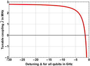
Figure 3: Variation of the dynamic tunable coupling $\tilde{J}$ w.r.t. the detuning $\Delta$ for each qubit. There exists a cutoff value, in this case $\Delta=-1.426$ GHz, corresponding to $\omega^{\text{off}}_{C_{ij}}=5.426$ GHz. For all configurations, such a cut-off value can always be obtained.

In conclusion, to switch on the qubit-qubit coupling as an edge in the network graph, one sets the respective edge coupler’s detuning to a reasonable (within the bandwidth) value via $\omega^{\text{on}}_{C_{ij}}$, yielding a limited $\tilde{J}(\omega^{\text{on}}_{C_{ij}})$. Then a PST can be performed by modulating only the couplers’ frequency to $\tilde{J}(\omega^{\text{on}}_{C_{ij}})$ for all the edges $E({\mathcal{Q}}_{d})$. Therefore,

$$\tilde{V}_{{\mathcal{Q}}_{n}}\xrightarrow{\text{switch off }E({\mathcal{Q}}_{n}-{\mathcal{Q}}_{d})}\tilde{V}_{\overline{{\mathcal{Q}}}_{n}\equiv{\mathcal{Q}}_{d}}$$ (19)

and the perfect state transfer time ($t_{0}$) is related to the dynamical coupling as $t_{0}=\pi/(2\tilde{J}^{\text{on}})$.

Fig. 3 shows the variation, Eqn. (18), of the dynamic tunable coupling $\tilde{J}$ with respect to the control parameter $\omega_{C_{ij}}$ through $\Delta$. The reasonable experimental values for the parameters used are ref:14 : $C_{i}=70$ fF, $C_{j}=72$ fF, $C_{c_{ij}}=200$ fF, $C_{ic_{ij}}=4$ fF, $C_{jc_{ij}}=4.2$ fF and $C_{ij}=0.1$ fF. All $\omega_{i}=\omega_{j}=\omega=4$ GHz (because all qubits are identical). The fabrication defects and imperfection is accounted in the different values for the capacitance. We have to ensure in the experiment that all detunings are onset to the same value to realise a uniformly coupled qubit hypercube ${\mathcal{Q}}_{d}$. If all detunings are not equal this will actually realise a weighted edge hypercube and introduce an error in the fidelity (see Appendix B). In one way, it can be first compensated by different values of the capacitive couplings involved. For the error that still remains, we can calculate the bound on the fidelity. For the case of example in Fig. 1 with ${\mathcal{Q}}_{n=4}$, that the maximum deviation in $\tilde{J}_{ij}$ for each edge is $\pm 0.5\%$, we have $\mathcal{F}>97.43\%$ (using Eqn. (B.8)).

V Conclusion

We proposed a switching procedure on a memory-enhanced hypercube such that an induced sub-hypercube can be determined with a desired pair of antipodal vertices of the hypercube. Consequently, we showed that the constructed sub-hypercube enables to provide support for perfect state transfer between any pair of distinct vertices of the hypercube. It is clear that the proposed method can be scaled up to any higher dimensional hypercube except the fact that the access and storage of the labelling of vertices of the hypercube can be done efficiently. A framework of superconducting qubits with tunable couplings is defined for physical implementation of the switching procedure under the XY coupling. It is shown that perfect state transfer between any pair of vertices in a hypercube is possible utilizing the proposed switching procedure. It will be an interesting exposure to extend this method for graphs that have structural support of construction of sub-hypercubes as subgraphs of the graph on any number vertices. We plan to work on this in future. Also, it will be equally interesting to propose a physical implementation of our protocol for the case of Heisenberg interaction where the z-z qubit couplings are required to be tunable. These questions remain to be addressed.

Appendix

Appendix A Effective Hamiltonian

In this appendix we derive the effective Hamiltonian (16) in the main text with the aim of decoupling the ancillary couplers from the computational qubits. Starting with the non-RWA Hamiltonian (12) and employing the Schrieffer-Wolff transformation (15) we obtain the most general Hamiltonian up to second order in $g_{i}/\Delta_{i}$ as

$$\begin{split}\frac{\tilde{H}_{{\mathcal{Q}}_{n}}}{\hbar}=&\frac{1}{2}\sum_{i=1}^{2^{n}}\omega_{i}\sigma^{z}_{i}+\frac{1}{2}\sum_{\langle i,j\rangle}\omega_{C_{ij}}\sigma^{z}_{C_{ij}}+\sum_{\langle i,j\rangle}g_{ij}\sigma^{x}_{i}\sigma^{x}_{j}+\sum_{\langle i,j\rangle}\Bigg{[}-\frac{g_{i}^{2}}{2}\Bigg{(}\frac{1}{\Delta_{i}}-\frac{1}{\Sigma_{i}}\Bigg{)}\left(\sigma^{+}_{i}\sigma^{+}_{j}+\sigma^{-}_{i}\sigma^{-}_{j}\right)\sigma^{z}_{C_{ij}}\\ &+\frac{g_{i}^{2}}{2}\Bigg{(}\frac{1}{\Delta_{i}}+\frac{1}{\Sigma_{i}}\Bigg{)}\sigma_{i}^{z}\sigma^{+}_{C_{ij}}\sigma^{+}_{C_{ij}}-\frac{g_{i}^{2}}{2}\Bigg{(}\frac{1}{\Delta_{i}}-\frac{1}{\Sigma_{i}}\Bigg{)}\sigma_{i}^{z}\sigma^{-}_{C_{ij}}\sigma^{-}_{C_{ij}}+\frac{g_{i}^{2}}{\Delta_{i}}\left(\sigma^{z}_{i}\sigma^{-}_{C_{ij}}\sigma^{+}_{C_{ij}}+\sigma^{-}_{i}\sigma^{+}_{i}\right)\\ &+\frac{g_{i}^{2}}{\Sigma_{i}}\left(\sigma^{z}_{i}\sigma^{-}_{C_{ij}}\sigma^{+}_{C_{ij}}-\sigma^{+}_{i}\sigma^{-}_{i}\sigma^{z}_{C_{ij}}\right)\Bigg{]}+\sum_{\begin{subarray}{c}\langle i,j\rangle\\ \langle i,k\rangle\end{subarray}}\Bigg{[}\frac{g_{i}^{2}}{2}\Bigg{(}\frac{1}{\Delta_{i}}-\frac{1}{\Sigma_{i}}\Bigg{)}\sigma_{i}^{z}\Big{(}\sigma^{-}_{C_{ij}}\sigma^{+}_{C_{ik}}-\sigma^{+}_{C_{ij}}\sigma^{-}_{C_{ik}}+\sigma^{-}_{C_{ij}}\sigma^{-}_{C_{ik}}\\ &-\sigma^{+}_{C_{ij}}\sigma^{+}_{C_{ik}}\Big{)}\Bigg{]}-\sum_{\langle i,j\rangle}\frac{g_{i}g_{j}}{2}\Bigg{(}\frac{1}{\Delta_{i}}+\frac{1}{\Delta_{j}}-\frac{1}{\Sigma_{i}}-\frac{1}{\Sigma_{j}}\Bigg{)}\left(\sigma^{+}_{i}\sigma^{+}_{j}+\sigma^{+}_{i}\sigma^{-}_{j}+\sigma^{-}_{i}\sigma^{+}_{j}+\sigma^{-}_{i}\sigma^{-}_{j}\right)\sigma^{z}_{C_{ij}}\end{split}$$ (A.1)

We now drop the terms which involve double excitation of either the qubits or the couplers and impose the strict condition that all couplers remain in their ground state. This completely decouples the coupler Hamiltonian which can be completely dropped. Further, all the constant energy shift terms can be neglected. This results in the following network Hamiltonian with renormalized frequencies

$$\begin{split}\frac{\tilde{H}_{{\mathcal{Q}}_{n}}}{\hbar}=\frac{1}{2}\sum_{i=1}^{2^{n}}\tilde{\omega}_{i}\sigma^{z}_{i}+\underbrace{\sum_{\langle i,j\rangle}\tilde{J}_{ij}\left(\sigma^{+}_{i}\sigma^{-}_{j}+\sigma^{-}_{i}\sigma^{+}_{j}\right)}_{\tilde{V}}\end{split}$$ (A.2)

where $\tilde{V}$ is the effective qubit-qubit interaction and

$$\tilde{\omega}_{i}\approx\omega_{i}+g^{2}_{i}\Bigg{(}\frac{1}{\Delta_{i}}+\frac{1}{\Sigma_{i}}\Bigg{)}$$ (A.3)

is the new corrected frequency due to the Lamb-shift frequency revealed by the SW transformation and

$$\tilde{J}_{ij}\approx\frac{g_{i}g_{j}}{2}\left(\frac{1}{\Delta_{i}}+\frac{1}{\Delta_{j}}-\frac{1}{\Sigma_{i}}-\frac{1}{\Sigma_{j}}\right)+g_{ij}.$$ (A.4)

is the effective and dynamic qubit-qubit coupling of the network qubits.

Appendix B Error calculation for non-ideal switching

Starting from the hypercube ${\mathcal{Q}}_{n}$, and switching to a graph $\overline{{\mathcal{Q}}}_{n}$ for a desired ${\mathcal{Q}}_{d}$, the switching may not be ideal. Meaning that the detuning parameters are not exact. This means that there can be edge strengths which are not exactly zero but coupled with some finite effective strength $\tilde{J}_{ij}\neq 0$ between the qubits $i$ and $j$ that are supposed to be decoupled. And also, there can be edges which are not all identically weighted as $\tilde{J}^{\text{on}}$. Therefore, the effective network graph adjacency matrix is weighted ($A^{\prime}(\overline{{\mathcal{Q}}}_{n})$). It is important to calculate the error bounds due to these experimental errors over the fidelity of PST. Here we look at such error independently. Eqn. (8) then takes the form

$$\begin{split}A^{\prime}(\overline{{\mathcal{Q}}}_{n})=&\left[\begin{matrix}A({\mathcal{Q}}_{d})+E({\mathcal{Q}}_{d})&E\\ E^{T}&E(\overline{{\mathcal{Q}}}_{d})\end{matrix}\right]\\ =&\left[\begin{matrix}A({\mathcal{Q}}_{d})&0\\ 0&0\end{matrix}\right]+\left[\begin{matrix}E({\mathcal{Q}}_{d})&E\\ E^{T}&E(\overline{{\mathcal{Q}}}_{d})\end{matrix}\right]=\mathcal{U}+\mathcal{E}\end{split}$$ (B.1)

where the $\mathcal{E}=[e_{ij}]$ (with $|e_{ij}|\ll|a_{ij}|$) is a matrix with small norm that captures the effect of unwanted edges. Then from konstantinov1996improved we have

$$\exp(-it(\mathcal{U}+\mathcal{E}))=\exp(-it\mathcal{U})+K(-it,\mathcal{E})$$ (B.2)

where

$$\begin{split}K(-it,\mathcal{E})&=\int_{0}^{t}\exp\left(-(it+s)\mathcal{U}\right)\mathcal{E}\exp\left(s(\mathcal{U}+\mathcal{E})\right)ds\\ &=\sum_{m=1}^{\infty}K_{m}(-it,\mathcal{E})\end{split}$$ (B.3)

and

$$\begin{split}K_{m}(-it,\mathcal{E})&=\int_{0}^{t}\exp(-(it+s)\mathcal{U})G_{m}(s,\mathcal{E})ds,\\ G_{m}(s,\mathcal{E})&=\sum_{r=m-1}^{\infty}\frac{s^{r}}{r!}\sum_{i_{1}+i_{2}+\ldots+i_{m}=r-m+1}\Pi_{k=1}^{m}(\mathcal{EU})^{i_{k}}\end{split}$$ (B.4)

Indeed,

$$\|K_{m}(-it,\mathcal{E})\|_{2}=\mathcal{O}(\|\mathcal{E}\|_{2}^{m})\leq\mathcal{O}(\|\mathcal{E}\|_{F}^{m})$$ (B.5)

where $\|M\|_{2}=\sum_{x\neq 0}\frac{\|Mx\|_{2}}{\|x\|_{2}},\|M\|_{F}=\left(\sum_{i,j=1}^{n}|m_{ij}|^{2}\right)^{1/2}$ for any matrix $M=[m_{ij}]$ of order $n\times n.$

Therefore,

$$\|K(-it,\mathcal{E})\|_{2}\leq\sum_{m=1}^{\infty}\mathcal{O}(\|\mathcal{E}\|_{F}^{m})$$ (B.6)

Then modulus inequality reveals that

$$|\langle y^{\prime}|e^{-it_{0}\mathcal{U}}|x^{\prime}\rangle+\langle y^{\prime}|K(-it_{0},\mathcal{E})|x^{\prime}\rangle|\geq 1-|\langle y^{\prime}|K(-it_{0},\mathcal{E})|x^{\prime}\rangle|.$$ (B.7)

Using Eqn. (B.6) equipped with Cauchy-Schwarz inequality gives the bound on the effective fidelity as

$$\mathcal{F}\geq 1-\sum_{m=1}^{\infty}\mathcal{O}(\|\mathcal{E}\|_{F}^{m}).$$ (B.8)

Therefore, all the inaccurate edge strengths give a compromise on the fidelity which is captured by this inequality, by simply knowing the estimate for strength of various effective coupling deviations in $\overline{{\mathcal{Q}}}_{n}$.

References

- [1] Charles H. Bennett and David P. DiVincenzo. Quantum information and computation. Nature, 404(6775):247–255, Mar 2000.
- [2] Alexandre Blais, Arne L. Grimsmo, S. M. Girvin, and Andreas Wallraff. Circuit Quantum Electrodynamics, 2020.
- [3] Anton Frisk Kockum and Franco Nori. Quantum Bits with Josephson Junctions, pages 703–741. Springer International Publishing, Cham, 2019.
- [4] J. Q. You and Franco Nori. Quantum information processing with superconducting qubits in a microwave field. Phys. Rev. B, 68:064509, Aug 2003.
- [5] J. Q. You and Franco Nori. Atomic physics and quantum optics using superconducting circuits. Nature, 474(7353):589–597, Jun 2011.
- [6] Iulia Buluta, Sahel Ashhab, and Franco Nori. Natural and artificial atoms for quantum computation. Reports on Progress in Physics, 74(10):104401, sep 2011.
- [7] Xiu Gu, Anton Frisk Kockum, Adam Miranowicz, Yu-xi Liu, and Franco Nori. Microwave photonics with superconducting quantum circuits. Physics Reports, 718-719:1–102, Nov 2017.
- [8] Alexandre Blais, Ren-Shou Huang, Andreas Wallraff, S. M. Girvin, and R. J. Schoelkopf. Cavity quantum electrodynamics for superconducting electrical circuits: An architecture for quantum computation. Phys. Rev. A, 69:062320, Jun 2004.
- [9] Joseph W. Britton, Brian C. Sawyer, Adam C. Keith, C.-C. Joseph Wang, James K. Freericks, Hermann Uys, Michael J. Biercuk, and John J. Bollinger. Engineered two-dimensional Ising interactions in a trapped-ion quantum simulator with hundreds of spins. Nature, 484(7395):489–492, Apr 2012.
- [10] Colin D. Bruzewicz, John Chiaverini, Robert McConnell, and Jeremy M. Sage. Trapped-ion quantum computing: Progress and challenges. Applied Physics Reviews, 6(2):021314, Jun 2019.
- [11] Rami Barends, Julian Kelly, Anthony Megrant, Andrzej Veitia, Daniel Sank, Evan Jeffrey, Ted C White, Josh Mutus, Austin G Fowler, Brooks Campbell, et al. Superconducting quantum circuits at the surface code threshold for fault tolerance. Nature, 508(7497):500–503, 2014.
- [12] M. W. Johnson, M. H. S. Amin, S. Gildert, T. Lanting, F. Hamze, N. Dickson, R. Harris, A. J. Berkley, J. Johansson, P. Bunyk, E. M. Chapple, C. Enderud, J. P. Hilton, K. Karimi, E. Ladizinsky, N. Ladizinsky, T. Oh, I. Perminov, C. Rich, M. C. Thom, E. Tolkacheva, C. J. S. Truncik, S. Uchaikin, J. Wang, B. Wilson, and G. Rose. Quantum annealing with manufactured spins. Nature, 473(7346):194–198, May 2011.
- [13] Lian-Ao Wu, Adam Miranowicz, XiangBin Wang, Yu-xi Liu, and Franco Nori. Perfect function transfer and interference effects in interacting boson lattices. Phys. Rev. A, 80:012332, Jul 2009.
- [14] Marcin Markiewicz and Marcin Wieśniak. Perfect state transfer without state initialization and remote collaboration. Phys. Rev. A, 79:054304, May 2009.
- [15] Daniel Burgarth, Vittorio Giovannetti, and Sougato Bose. Efficient and perfect state transfer in quantum chains. Journal of Physics A: Mathematical and General, 38(30):6793–6802, jul 2005.
- [16] Hannes Bernien, Sylvain Schwartz, Alexander Keesling, Harry Levine, Ahmed Omran, Hannes Pichler, Soonwon Choi, Alexander S. Zibrov, Manuel Endres, Markus Greiner, Vladan Vuletić, and Mikhail D. Lukin. Probing many-body dynamics on a 51-atom quantum simulator. Nature, 551(7682):579–584, Nov 2017.
- [17] Chao Song, Kai Xu, Wuxin Liu, Chui-ping Yang, Shi-Biao Zheng, Hui Deng, Qiwei Xie, Keqiang Huang, Qiujiang Guo, Libo Zhang, Pengfei Zhang, Da Xu, Dongning Zheng, Xiaobo Zhu, H. Wang, Y.-A. Chen, C.-Y. Lu, Siyuan Han, and Jian-Wei Pan. 10-Qubit Entanglement and Parallel Logic Operations with a Superconducting Circuit. Phys. Rev. Lett., 119:180511, Nov 2017.
- [18] Julian Kelly, Rami Barends, Austin G Fowler, Anthony Megrant, Evan Jeffrey, Theodore C White, Daniel Sank, Josh Y Mutus, Brooks Campbell, Yu Chen, et al. State preservation by repetitive error detection in a superconducting quantum circuit. Nature, 519(7541):66–69, 2015.
- [19] David P. DiVincenzo. The Physical Implementation of Quantum Computation. Fortschritte der Physik, 48(9-11):771–783, Sep 2000.
- [20] Sougato Bose. Quantum Communication through an Unmodulated Spin Chain. Phys. Rev. Lett., 91(207901), Nov 2003.
- [21] Tobias J. Osborne. Statics and dynamics of quantum and Heisenberg systems on graphs. Phys. Rev. B, 74:094411, Sep 2006.
- [22] Alastair Kay. Basics of perfect communication through quantum networks. Phys. Rev. A, 84:022337, Aug 2011.
- [23] Ashok Ajoy and Paola Cappellaro. Mixed-state quantum transport in correlated spin networks. Phys. Rev. A, 85:042305, Apr 2012.
- [24] Alastair Kay. Perfect, efficient, state transfer and its applications as a constructive tool. International Journal of Quantum Information, 08(04):641–676, Jun 2010.
- [25] V. Subrahmanyam. Entanglement dynamics and quantum-state transport in spin chains. Phys. Rev. A, 69:034304, Mar 2004.
- [26] Antoni Wojcik, Tomasz Luczak, Pawel Kurzynski, Andrzej Grudka, Tomasz Gdala, and Malgorzata Bednarska. Multiuser quantum communication networks. Phys. Rev. A, 75:022330, Feb 2007.
- [27] Gabriel Coutinho and Henry Liu. No Laplacian Perfect State Transfer in Trees. SIAM Journal on Discrete Mathematics, 29(4):2179–2188, Jan 2015.
- [28] Ethan Ackelsberg, Zachary Brehm, Ada Chan, Joshua Mundinger, and Christino Tamon. Laplacian state transfer in coronas. Linear Algebra and its Applications, 506:154 – 167, 2016.
- [29] Rúben Sousa and Yasser Omar. Pretty good state transfer of entangled states through quantum spin chains. New Journal of Physics, 16(12):123003, dec 2014.
- [30] Leonardo Banchi, Gabriel Coutinho, Chris Godsil, and Simone Severini. Pretty good state transfer in qubit chains - The Heisenberg Hamiltonian. Journal of Mathematical Physics, 58(3):032202, 2017.
- [31] Alastair Kay. Perfect and Pretty Good State Transfer for Field-Free Heisenberg Chains, 2019.
- [32] Wayne Jordan Chetcuti, Claudio Sanavio, Salvatore Lorenzo, and Tony J G Apollaro. Perturbative many-body transfer. New Journal of Physics, 22(3):033030, mar 2020.
- [33] Leonardo Banchi, Abolfazl Bayat, Paola Verrucchi, and Sougato Bose. Nonperturbative Entangling Gates between Distant Qubits Using Uniform Cold Atom Chains. Phys. Rev. Lett., 106:140501, Apr 2011.
- [34] Vivien M. Kendon and Christino Tamon. Perfect State Transfer in Quantum Walks on Graphs. 2011.
- [35] John Brown, Chris Godsil, Devlin Mallory, Abigail Raz, and Christino Tamon. Perfect State Transfer on Signed Graphs. Quantum Info. Comput., 13(5–6):511–530, May 2013.
- [36] Chris Godsil and Sabrina Lato. Perfect State Transfer on Oriented Graphs, 2020.
- [37] Marzieh Asoudeh and Vahid Karimipour. Perfect state transfer on spin-1 chains. Quantum Information Processing, 13(3):601–614, Mar 2014.
- [38] Jafarizadeh M.A., Sufiani R., Azimi M., and et. al. Perfect state transfer over interacting boson networks associated with group schemes. Quantum Inf Process, 11:171–187, 2012.
- [39] Frank Arute, Kunal Arya, Ryan Babbush, Dave Bacon, Joseph C. Bardin, Rami Barends, Rupak Biswas, Sergio Boixo, Fernando G. S. L. Brandao, David A. Buell, Brian Burkett, Yu Chen, Zijun Chen, Ben Chiaro, Roberto Collins, William Courtney, Andrew Dunsworth, Edward Farhi, Brooks Foxen, Austin Fowler, Craig Gidney, Marissa Giustina, Rob Graff, Keith Guerin, Steve Habegger, Matthew P. Harrigan, Michael J. Hartmann, Alan Ho, Markus Hoffmann, Trent Huang, Travis S. Humble, Sergei V. Isakov, Evan Jeffrey, Zhang Jiang, Dvir Kafri, Kostyantyn Kechedzhi, Julian Kelly, Paul V. Klimov, Sergey Knysh, Alexander Korotkov, Fedor Kostritsa, David Landhuis, Mike Lindmark, Erik Lucero, Dmitry Lyakh, Salvatore Mandrà , Jarrod R. McClean, Matthew McEwen, Anthony Megrant, Xiao Mi, Kristel Michielsen, Masoud Mohseni, Josh Mutus, Ofer Naaman, Matthew Neeley, Charles Neill, Murphy Yuezhen Niu, Eric Ostby, Andre Petukhov, John C. Platt, Chris Quintana, Eleanor G. Rieffel, Pedram Roushan, Nicholas C. Rubin, Daniel Sank, Kevin J. Satzinger, Vadim Smelyanskiy, Kevin J. Sung, Matthew D. Trevithick, Amit Vainsencher, Benjamin Villalonga, Theodore White, Z. Jamie Yao, Ping Yeh, Adam Zalcman, Hartmut Neven, and John M. Martinis. Quantum supremacy using a programmable superconducting processor. Nature, 574(7779):505–510, Oct 2019.
- [40] J. I. Cirac and P. Zoller. Quantum Computations with Cold Trapped Ions. Phys. Rev. Lett., 74:4091–4094, May 1995.
- [41] Alexandre Blais, Jay Gambetta, A. Wallraff, D. I. Schuster, S. M. Girvin, M. H. Devoret, and R. J. Schoelkopf. Quantum-information processing with circuit quantum electrodynamics. Phys. Rev. A, 75:032329, Mar 2007.
- [42] Yu-xi Liu, C. P. Sun, and Franco Nori. Scalable superconducting qubit circuits using dressed states. Physical Review A, 74(5), Nov 2006.
- [43] X. Li, Y. Ma, J. Han, Tao Chen, Y. Xu, W. Cai, H. Wang, Y.P. Song, Zheng-Yuan Xue, Zhang-qi Yin, and Luyan Sun. Perfect Quantum State Transfer in a Superconducting Qubit Chain with Parametrically Tunable Couplings. Phys. Rev. Applied, 10:054009, Nov 2018.
- [44] Matthias Christandl, Nilanjana Datta, Artur Ekert, and Andrew J. Landahl. Perfect State Transfer in Quantum Spin Networks. Phys. Rev. Lett., 92:187902, May 2004.
- [45] Matthias Christandl, Nilanjana Datta, Tony C. Dorlas, Artur Ekert, Alastair Kay, and Andrew J. Landahl. Perfect transfer of arbitrary states in quantum spin networks. Phys. Rev. A, 71:032312, Mar 2005.
- [46] Sougato Bose, Andra Casaccino, Stefano Mancini, and Simone Severini. Communication in XYZ All-to-All Quantum Networks with a Missing Link. International Journal of Quantum Information, 07(04):713–723, 2009.
- [47] Christopher Facer, Jason Twamley, and James Cresser. Quantum Cayley networks of the hypercube. Physical Review A, 77(1), Jan 2008.
- [48] Simone Paganelli, Salvatore Lorenzo, Tony J. G. Apollaro, Francesco Plastina, and Gian Luca Giorgi. Routing quantum information in spin chains. Phys. Rev. A, 87:062309, Jun 2013.
- [49] Antoni Wojcik, Tomasz Luczak, Pawel Kurzynski, Andrzej Grudka, Tomasz Gdala, and Malgorzata Bednarska. Unmodulated spin chains as universal quantum wires. Phys. Rev. A, 72:034303, Sep 2005.
- [50] Rozhin Yousefjani and Abolfazl Bayat. Simultaneous multiple-user quantum communication across a spin-chain channel. Phys. Rev. A, 102:012418, Jul 2020.
- [51] Douglas Brent West et al. Introduction to graph theory, volume 2. Prentice hall Upper Saddle River, 2001.
- [52] Vivien M Kendon and Christino Tamon. Perfect state transfer in quantum walks on graphs. Journal of Computational and Theoretical Nanoscience, 8(3):422–433, 2011.
- [53] John Brown, Chris Godsil, Devlin Mallory, Abigail Raz, and Christino Tamon. Perfect State Transfer on Signed Graphs. Quantum Info. Comput., 13(5-6):511–530, May 2013.
- [54] Andrew S Tanenbaum. Structured computer organization. Pearson Education India, 2016.
- [55] David A Patterson and John L Hennessy. Computer Organization and Design ARM Edition: The Hardware Software Interface. Morgan kaufmann, 2016.
- [56] Maurizio Gabbrielli and Simone Martini. Programming languages: principles and paradigms. Springer Science & Business Media, 2010.
- [57] Colin P Williams. Explorations in quantum computing. Springer Science & Business Media, 2010.
- [58] Gavin Brennen, Elisabeth Giacobino, and Christoph Simon. Focus on quantum memory. New Journal of Physics, 17(5):050201, 2015.
- [59] Khabat Heshami, Duncan G England, Peter C Humphreys, Philip J Bustard, Victor M Acosta, Joshua Nunn, and Benjamin J Sussman. Quantum memories: emerging applications and recent advances. Journal of modern optics, 63(20):2005–2028, 2016.
- [60] Dawoud Shenouda Dawoud and R Peplow. Digital System Design: Use of Microcontroller, volume 2. River Publishers, 2010.
- [61] D. Rosenberg, D. Kim, R. Das, D. Yost, S. Gustavsson, D. Hover, P. Krantz, A. Melville, L. Racz, G. O. Samach, S. J. Weber, F. Yan, J. L. Yoder, A. J. Kerman, and W. D. Oliver. 3D integrated superconducting qubits. npj Quantum Information, 3(1):42, Oct 2017.
- [62] V. Karimipour, M. Sarmadi Rad, and M. Asoudeh. Perfect quantum state transfer in two- and three-dimensional structures. Phys. Rev. A, 85:010302, Jan 2012.
- [63] Salvatore S. Elder, Christopher S. Wang, Philip Reinhold, Connor T. Hann, Kevin S. Chou, Brian J. Lester, Serge Rosenblum, Luigi Frunzio, Liang Jiang, and Robert J. Schoelkopf. High-Fidelity Measurement of Qubits Encoded in Multilevel Superconducting Circuits. Phys. Rev. X, 10:011001, Jan 2020.
- [64] Yu Chen, C. Neill, P. Roushan, N. Leung, M. Fang, R. Barends, J. Kelly, B. Campbell, Z. Chen, B. Chiaro, A. Dunsworth, E. Jeffrey, A. Megrant, J. Y. Mutus, P. J. J. O’Malley, C. M. Quintana, D. Sank, A. Vainsencher, J. Wenner, T. C. White, Michael R. Geller, A. N. Cleland, and John M. Martinis. Qubit Architecture with High Coherence and Fast Tunable Coupling. Physical Review Letters, 113(22), November 2014.
- [65] Fei Yan, Philip Krantz, Youngkyu Sung, Morten Kjaergaard, Daniel L. Campbell, Terry P. Orlando, Simon Gustavsson, and William D. Oliver. Tunable Coupling Scheme for Implementing High-Fidelity Two-Qubit Gates. Phys. Rev. Applied, 10:054062, Nov 2018.
- [66] Georg M. Reuther, David Zueco, Frank Deppe, Elisabeth Hoffmann, Edwin P. Menzel, Thomas Weißl, Matteo Mariantoni, Sigmund Kohler, Achim Marx, Enrique Solano, Rudolf Gross, and Peter Hänggi. Two-resonator circuit quantum electrodynamics: Dissipative theory. Physical Review B, 81(14), April 2010.
- [67] Youngkyu Sung, Leon Ding, Jochen Braumüller, Antti Vepsäläinen, Bharath Kannan, Morten Kjaergaard, Ami Greene, Gabriel O. Samach, Chris McNally, David Kim, Alexander Melville, Bethany M. Niedzielski, Mollie E. Schwartz, Jonilyn L. Yoder, Terry P. Orlando, Simon Gustavsson, and William D. Oliver. Realization of high-fidelity CZ and ZZ-free iSWAP gates with a tunable coupler, 2020.
- [68] David Zueco, Georg M. Reuther, Sigmund Kohler, and Peter Hänggi. Qubit-oscillator dynamics in the dispersive regime: Analytical theory beyond the rotating-wave approximation. Phys. Rev. A, 80:033846, Sep 2009.
- [69] M. D. Jenkins, D. Zueco, O. Roubeau, G. Aromí, J. Majer, and F. Luis. A scalable architecture for quantum computation with molecular nanomagnets. Dalton Trans., 45:16682–16693, 2016.
- [70] Mihail Konstantinov, Petko Petkov, Parashkeva Gancheva, Vera Angelova, and Ivan Popchev. Improved perturbation bounds for the matrix exponential. In International Workshop on Numerical Analysis and Its Applications, pages 258–265. Springer, 1996.