Cosmic Reionization May Still Have Started Early and Ended Late: Confronting Early Onset with CMB Anisotropy and 21 cm Global Signals

Abstract

The global history of reionization was shaped by the relative amounts of starlight released by three halo mass groups: atomic-cooling halos (ACHs) with virial temperatures $T_{{\rm vir}}>10^{4}\,{\rm K}$, either (1) massive enough to form stars even after reionization (HMACHs, $\gtrsim 10^{9}\,M_{\odot}$) or (2) less-massive (LMACHs), subject to star formation suppression when overtaken by reionization, and (3) ${\rm H_{2}}$-cooling minihalos (MHs) with $T_{{\rm vir}}<10^{4}\,{\rm K}$, whose star formation is predominantly suppressed by the ${\rm H_{2}}$-dissociating Lyman-Werner (LW) background. Our previous work showed that including MHs caused two-stage reionization – early rise to $x\lesssim 0.1$, driven by MHs, followed by a rapid rise, late, to $x\sim 1$, driven by ACHs – with a signature in CMB polarization anisotropy predicted to be detectable by the Planck satellite. Motivated by this prediction, we model global reionization semi-analytically for comparison with Planck CMB data and the EDGES global 21cm absorption feature, for models with: (1) ACHs, no feedback; (2) ACHs, self-regulated; and (3) ACHs and MHs, self-regulated. Model (3) agrees well with Planck E-mode polarization data, even with a substantial tail of high-redshift ionization, beyond the limit proposed by the Planck Collaboration (2018). No model reproduces the EDGES feature. For model (3), $\left|\delta T_{b}\right|\lesssim 60\,{\rm mK}$ across the EDGES trough, an order of magnitude too shallow, and absorption starts at higher $z$ but is spectrally featureless. Early onset reionization by Population III stars in MHs is compatible with current constraints, but only if the EDGES interpretation is discounted or else other processes we did not include account for it.

1 Introduction

Cosmic reionization is commonly believed to have commenced with the birth of first stars in the Universe and ended when all the intergalactic medium (IGM) became ionized due to the net production of ionizing-photons surpassing the number of neutral hydrogen atoms. This whole epoch marks the epoch of reionization (EoR) in the history of the Universe. There exist several observational constraints, including (1) the quasar Gunn-Peterson trough (Becker et al. 2001; Fan et al. 2002): reionization is likely to have ended at $z\gtrsim 6$, (2) the temporal evolution of the 21 cm background at redshift $z\sim 6$ (Bowman & Rogers 2010): a sudden reionization scenario is ruled out, (3) the polarization anisotropy of the cosmic microwave background (CMB)(Planck Collaboration et al. 2018): the optical depth to the CMB photon, $\tau_{{\rm es}}$, is $0.054_{-0.0081}^{+0.0070}$($1\sigma$), (4) the sudden change of the Ly$\alpha$-emitter (LAE) population (Pentericci et al. 2011): the global ionized fraction, $x$, at $z\simeq 7$ is at least $\gtrsim 0.1$, (5) the quasar proximity effect (Calverley et al. 2011): the metagalactic ionization rate $\Gamma$ at $z\simeq 6$ is about $10^{-13}\,{\rm s^{-1}}$. These constrains are nevertheless insufficient to constrain the full history of reionization.

Constraining the cosmic reionization process by observations requires theoretical modelling, of course. The simplest approach is to calculate the history of reionization using semi-analytical, one-zone models (see e.g. Haardt & Madau 1996; Haiman & Loeb 1997; Haiman & Holder 2003; Furlanetto 2006). The more difficult approach is to simulate the process numerically (see e.g. Iliev et al. 2007; Trac & Cen 2007; Kohler et al. 2007; Mesinger et al. 2011). These methods are mutually complementary. For example, the former allows a very fast exploration of the parameter space, while the latter enables simulating the 3-dimensional (3D) structure of the process. If one is interested only in the averaged quantities, such as the global ionized fraction $x$ and the kinetic temperature of the intergalactic medium (IGM) $T_{k}$, the one-zone calculation can provide surprisingly reliable estimates very easily. Therefore the one-zone calculation has been used quite extensively. This method has become very useful in reionization-parameter estimation effort, while one has to be wary about the fact that such an estimation is limited to specific reionization models that are assumed to be fully described by those parameters.

Some of the semi-analytical one-zone modellings used to have common “conventions”: (1) only atomic-cooling halos, with virial temperature $T_{{\rm vir}}\gtrsim 10^{4}\,{\rm K}$, are considered as radiation sources, (2) the star formation rate (SFR) is proportional to the growth rate $df_{{\rm coll}}/dt$ of the halo-collapsed fraction $f_{{\rm coll}}$, and (3) feedback effects are neglected (Loeb & Barkana 2001; Furlanetto 2006; Pritchard & Furlanetto 2006). We categorize those models that follow these conventions as the vanilla model. First, main justification for the first convention is from the fact that stars inside less-massive halos, or minihalos (with $T_{{\rm vir}}\lesssim 10^{4}\,{\rm K}$ and mass limited down to the Jeans mass of the intergalactic medium), are susceptible to the Lyman-Werner feedback effect and the Jeans-mass filtering. The Lyman-Werner feedback strongly regulates the amount of ${\rm H}_{2}$ inside minihalos, the main cooling agent in the primordial environment, by photo-dissociation. The Jeans-mass filtering can happen if minihalos are exposed to the hydrogen-ionizing radiation field, either from inside or from outside. Therefore, their contribution was believed to be negligible. Second, justification for SFR $\propto df_{{\rm coll}}/dt$ is not solid, and this assumption is equivalent of null duty cycle of star formation (Section 2.1). Third, neglecting the feedback effect is a conventional simplification, while there may exist atomic-cooling halos in the low-mass end that are affected by the Jeans-mass filtering if embedded in photoionized regions (Section 2.2.2).

Many numerical simulations inherited the convention of neglecting minihalos, usually in those using a large ($\gtrsim$ a few tens of comoving Mpc) simulation box. While the justification is the strong LW feedback effect, a practical reason is the numerical resolution limit that becomes worse as the size of the simulation box becomes larger. Therefore, large-scale simulations of reionization usually suffers from this limit. To overcome this limit and include the impact of minihalo stars, a sub-grid treatment of missing halos (Ahn et al. 2015; Nasirudin et al. 2020) was included in a large simulation box by Ahn et al. (2012). They used an empirical, deterministic bias of minihalo population for any given density environment, to successfully populate minihalos over the domain of calculation. Using theoretical predictions on the formation of first stars inside minihalos, together with the impact of the LW feedback, they could then cover the fully dynamic range of halos. They found that (1) minihalo stars cannot finish reionization but can ionize the universe up to $\sim 20\,\%$ depending on the mass of Population III (Pop III) stars, (2) the resulting reionization history is composed of the early staggered stage with slow growth of $\left\langle x\right\rangle$ and the late rapid stage with rapid growth of $\left\langle x\right\rangle$, (3) the reionization is finished by photons from atomic-cooling halos, and (4) there exist degeneracy in reionization histories that can result in the same $\tau_{{\rm es}}$ and $z_{{\rm reion}}$.

There exists an interesting hint from the recent large-scale CMB polarization observation that is related to the result by Ahn et al. (2012). Constraining the full history of reionization has become available only recently, through observation of the large-scale CMB polarization anisotropy. Having such constraints used to be impossible with the given quality of CMB polarization data before, and thus only a two-parameter constraint on reionization with $\tau_{{\rm es}}$ and the reionization redshift $z_{{\rm reion}}$ had been available (e.g. Hinshaw et al. 2013; Planck Collaboration et al. 2013). The Planck 2015 data (Planck Collaboration et al. 2016) first allowed constraining the history of reionization beyond this two-parameter constraint, and it was claimed that the Planck data favored a type of reionization histories composed of (1) the early, slow growth of $x$ for a large range of redshift $z\sim 30-10$ and (2) the late, rapid growth of $x$ for a short range of redshift $z\sim 10-6$ (Miranda et al. 2017; Heinrich & Hu 2018). While criticisms on this claim appeared due to the limitation of having only the Planck Low Frequency Instrument (LFI) data (Millea & Bouchet 2018), this “two-stage” reionization histories had been indeed predicted by Ahn et al. (2012), in which the early stage is dominated by strongly self-regulated formation of stars inside minihalos, presumably Pop III stars, and the late stage by stars inside atomically-cooling halos, presumably Population II (Pop II) stars, with weaker (inside low-mass atomic cooling halos, LMACHs) or even no modulation (inside high-mass atomic cooling halos, HMACHs) on star formation. The most refined, non-parametric constraint comes from the Planck 2018 observation that also includes the High Frequency Instrument (HFI) data (Planck Collaboration et al. 2018; Millea & Bouchet 2018), and the constraint bears qualitative similarity with but some quantitative difference from the analyses by Miranda et al. (2017) and Heinrich & Hu (2018). First, the two-stage reionization is still favored at $\lesssim 2\sigma$ level. Second, a “significant” amount of ionization at $z\gtrsim 15$ is disfavored, with maximum of $\sim 10\%$ ionized fraction allowed at $z\sim 15$ at 1$\sigma$ level. Even though Planck Collaboration et al. (2018) and Millea & Bouchet (2018) stress the latter finding and even claim that the early stage of reionization dominated by self-regulated Pop III stars is strongly disfavored, their constraint indeed allows very extended ionization histories reaching to $z\sim 25$ and $z\sim 30$ for the 1$\sigma$ and the $2\sigma$ constraint, respectively, in addition to showing a two-stage reionization feature. Therefore, we take the analysis on the Planck 2018 data (Planck Collaboration et al. 2018; Millea & Bouchet 2018) as a mild proof for the two-stage reionization, which will be tested quantitatively in this paper.

Meanwhile, observing the hydrogen 21 cm line background is believed to provide a direct probe of the the Dark Ages and the epoch of reionization. The deepest ($z=14-26$) observation so far, in terms of the sky-averaged global 21 cm background, has been delivered by the Experiment to Detect the Global Epoch of Reionization (EDGES), and the detection of $\sim 500\,{\rm mK}$ continuum absorption of the hydrogen 21-cm signal against the smooth background around $z\sim 17$ was claimed (Bowman et al. 2018). It is hard to grasp such a large absorption in the standard picture, compared to the maximum $\sim 200\,{\rm mK}$ depth allowed in the $\Lambda$CDM universe. The overall shape of the signal over the redshift range is also incompatible with usual model predictions. This “conflict” stimulated many resolutions, which fall into roughly three categories: (1) the analysis of removing a smooth galactic foreground and obtaining another smooth absorption signal is unreliable (Hills et al. 2018), (2) non-standard models beyond $\Lambda$CDM should be considered, such as large baryon-dark matter interaction (Tashiro et al. 2014; Barkana 2018) and abnormally large expansion rate at high redshift (Hill & Baxter 2018), and (3) the contribution of yet unknown sources to the radio continuum (the “excess radio background”) but still in the standard $\Lambda$CDM framework, may generate such a large absorption signal (e.g. Feng & Holder 2018; Ewall-Wice et al. 2018).

Motivated by the hint on the two-stage reionization from the Planck 2018 data and the compelling EDGES observation, we explore the possibility for the two-stage reionization to leave any characteristic signature in the CMB and the global 21 cm background. Toward this end, we use semi-analytical one-zone models to cover a wide range of reionization scenarios. We cast reionization models into three categories, from the vanilla model without feedback effect to progressively sophisticated ones, expanding the star-hosting halo species and considering feedback effects that regulate star formation in those halos. We then investigate how the history of reionization and the evolution of other relevant radiation fields shape the CMB the 21cm background, with special focus on finding whether the two-phase reionization models that carry the high-redshift ionization tail, constructed by the LW-regulated star formation in MHs, will leave any imprint on the CMB and the 21 cm background. While it is worthwhile to include the resolutions, alternative to the standard picture, for the deep absorption signal of the EDGES in the parameter estimation effort (Mirocha et al. 2018; Mirocha & Furlanetto 2019; Mebane et al. 2020; Qin et al. 2020a, 2021), we limit our study to the standard $\Lambda$CDM framework without the excess radio background and other alternatives but instead explore any new possible observational predictions. We indeed find out very unique and novel features of the two-phase ionization models both in the CMB and the global $\delta T_{{\rm b}}$, opening up exciting observational prospects.

The paper is organized as follows. In Section 2, we describe the details of the one-zone model, including the model categories and the numerical method. In Section 3, we present the estimates on the ionized fraction, the CMB polarization anisotropy and the 21 cm background for various reionization models, with special focus on the estimate from the strongly self-regulated models. We summarize and discuss the result in Section 4. Throughout this paper, we use cMpc to denote “comoving megaparsec”, or the comoving length in units of Mpc.

2 Method

We take a simple one-zone model for studying the global evolution of the physical states of IGM and backgrounds including the 21 cm signal. Two crucial parameters are $x$ and $T_{k}$, whose evolutions will be governed by physical properties, the evolution and the feedback of radiation sources. Therefore, the main equations for reionization models are the rate equations for $x$ and $T_{k}$.

The ionizing-photon production rate per baryon (PPR) is the source term that increases $x$, or the source term in the rate equation $dx/dt$ where $t$ is the cosmic time. PPR is the main parameter whose variance leads to the variance in the histories of reionization among different models. PPR during EoR is quite uncertain and will be parameterized by the species of host halos, spectral shape and the star formation duty cycle. PPR is also affected by various feedback effects. These will be the main subjects to be described in Sections 2.1 - 2.2.

The recombination rate is the sink term in the ionization equation. The recombination rate does not have the model variance as large as PPR. Nevertheless, there exists some uncertainty in the recombination rate mainly due to the difficulty in quantifying the clumping factor. We conservatively take a combination of previous studies that quantified the clumping factor.

A few radiation background fields are crucial in determining $T_{k}$ and the 21 cm spin temperature $T_{s}$. Variance in $T_{k}$ is caused by variance in the heating efficiency, and variance in $T_{s}$ by variance in Lyman-resonance-line backgrounds. Therefore, the model variance will be reflected also in the 21 cm background, which will be described in Sections 2.3 - 2.4. We defer the description of the used spectral energy distributions (SED) of the stellar radiation, which cause the variance in $T_{s}$ even at a similar level of the ionization state, to Sections 3.1 and 3.3.

Throughout this paper, we use cosmological parameters reported by Planck Collaboration et al. (2018): $h=0.6732$, $\Omega_{m,\,0}=0.3144$, $\Omega_{b,\,0}=0.04939$, $n_{s}=0.966$, and $\sigma_{8}=0.812$, which are the present Hubble parameter in the unit of $100\,{\rm km\,s^{-1}\,Mpc}$, the present matter density in units of the critical density, the present baryon density in units of the critical density, the power index of the primordial curvature perturbation, and the present variance of matter density at the filtering scale of $8h^{-1}\,{\rm Mpc}$. We use the mass function by Sheth & Tormen (1999) when calculating the halo-collapsed fraction.

2.1 Star formation rate density and duty cycle

It is a usual approximation that PPR is proportional to the star formation rate density (SFRD: star formation rate per comoving volume, in units of $M_{\odot}\,{\rm s^{-1}\,cMpc^{-3}}$). Rigorously, this becomes true only if $t_{*}$, the lifetime of stars which we take as a constant for a given stellar species (e.g. Pop II stars), is infinitesimal compared to the ionization time, i.e. $x/(dx/dt)$. Even more rigorously, for PPR at time $t$ to be the ionization rate at $t$, the photon travel time inside H II regions should also be very small. In this paper, we take this usual assumption, PPR $\propto$SFRD, that has been used extensively in semi-analytical modelling. The ionization rate $\xi$ (in the unit of ${\rm s}^{-1}$) will then be given by

$$\xi=f_{{\rm esc}}{\rm PPR}=f_{{\rm esc}}N_{{\rm ion}}\frac{{\rm SFRD}}{m_{b}n_{b,\,0}},$$ (1)

where $f_{{\rm esc}}$, $N_{{\rm ion}}$, $m_{b}$, $n_{b,\,0}$ are the ionizing-photon escape fraction out of halos, the total number of ionizing photons emitted per stellar baryon during the lifetime of a star, the baryon mass, and the average comoving baryon number density, respectively.

We also modify the typical assumption of semi-analytical calculations to incorporate non-zero duty cycle of star formation. Let us first briefly review the typical assumption in semi-analytical calculations: PPR and SFRD are assumed proportional to $df_{{\rm coll}}/dt$, the growth rate of the halo-collapsed fraction $f_{{\rm coll}}$, such that

$$\xi(t) =\xi_{{\rm a}}(t)=f_{*}f_{{\rm esc}}\frac{N_{{\rm ion}}}{t_{*}}\int_{t-t_{*}}^{t}dt^{\prime}\,\frac{df_{{\rm coll}}}{dt^{\prime}}$$

$$\simeq f_{*}f_{{\rm esc}}N_{{\rm ion}}\frac{df_{{\rm coll}}}{dt}(t)=f_{\gamma}\frac{df_{{\rm coll}}}{dt}(t),$$ (2)

where $\xi_{{\rm a}}$ denotes the ionization rate due to newly “accreted” matter, $f_{*}$ is the star formation efficiency in such an episode (e.g. Loeb & Barkana 2001; Furlanetto 2006), and $f_{\gamma}\equiv f_{*}f_{{\rm esc}}N_{{\rm ion}}$ is the proportionality coefficient between $\xi$ and $df_{{\rm coll}}/dt$. The second equality in equation (2) is a rigorous form that considers only the newly accreted matter, whose maximal lookback time in the integration should be $t_{*}$. Therefore, we can denote this assumption as the “mass-accretion dominated star formation” scenario (MADSF). In the limit of infinitesimal $t_{*}$ or slowly-varying $f_{{\rm coll}}$, the last approximation becomes valid. Because $df_{{\rm coll}}$ in equation (2) is the amount of matter that has been newly accreted into halos per time interval $dt$, considering $\xi_{{\rm a}}(t)$ only is identical to having null duty cycle such that any gas that has once formed stars can never form stars again. Note also that $df_{{\rm coll}}$ does not include halos whose mass has increased by a merger event at $t$, even though in nature “wet merger” events occur quite frequently. Because this null duty cycle assumption is somewhat extreme, we need to consider a more general case of non-zero duty cycle.

We quantity the non-zero duty cycle as the time fraction that stars emit radiation, $f_{{\rm DC}}\equiv t_{*}/(t_{*}+t_{{\rm dorm}})$, where $t_{{\rm dorm}}$ is the duration that a stellar baryon remains dormant after the death of the host star until a new star formation episode occurs. The same account on $t_{{\rm dorm}}$ has been addressed by Mirocha et al. (2018). Both $t_{*}$ and $t_{{\rm dorm}}$ are average quantities, and consequently $f_{{\rm DC}}$ will be a global parameter. Ergodicity is assumed such that this temporal duty cycle is the same as the spatially averaged fraction of gas that has once resided inside a star and now resides in a post-generation star. In this work, we further assume that $f_{{\rm DC}}$ is constant over time for a given stellar species. With non-zero $f_{{\rm DC}}$, we obtain the ionization rate $\xi_{{\rm d}}$ due to “duty cycle”:

$$\xi_{{\rm d}}(t) =f_{*}f_{{\rm esc}}f_{{\rm DC}}f_{{\rm coll}}(t-t_{*})\frac{N_{{\rm ion}}}{t_{*}}$$

$$\simeq f_{*}f_{{\rm esc}}f_{{\rm DC}}f_{{\rm coll}}(t)\frac{N_{{\rm ion}}}{t_{*}}=f_{*,{\rm d}}f_{{\rm esc}}f_{{\rm coll}}(t)\frac{N_{{\rm ion}}}{t_{*}},$$ (3)

where only “old” gas at lookback time $t_{*}$ is allowed to re-generate stars and the approximation holds when $t_{*}$ is treated infinitesimal. The last equality absorbs $f_{{\rm DC}}$ into the effective $f_{*}$ of halo gas, $f_{*,{\rm d}}$. Equation (3) obviously does not account for any newly accreted gas. Note also that equation (3) holds due to ergodicity: $f_{*,{\rm d}}$ is a spatially averaged quantity over many galaxies, which will be identical to the time average of star formation episodes on a single galaxy. We denote a scenario based on $\xi=\xi_{{\rm d}}$ as the “all-halo replenished star formation” scenario (AHRSF).

The most generic form for $\xi$ should implement both contributions from old gas and newly accreted gas, or combining the episodes of MADSF and AHRSF, such that

$$\xi=\xi_{{\rm d}}+\xi_{{\rm a}}=f_{*,{\rm d}}f_{{\rm esc}}f_{{\rm coll}}\frac{N_{{\rm ion}}}{t_{*}}+f_{*,{\rm a}}f_{{\rm esc}}N_{{\rm ion}}\frac{df_{{\rm coll}}}{dt},$$ (4)

where $f_{*}$ of newly accreted gas is denoted by $f_{*,{\rm a}}$, to be distinguished from $f_{*,{\rm d}}$. $f_{*,{\rm a}}=0$ corresponds to the case where newly accreted gas waits longer than $t_{*}$ to start star formation activity, and practically there is no theoretical constraint on the relative strengths of $f_{*,{\rm a}}$ over $f_{*,{\rm d}}$. With equation (4), both cases of $\xi\propto f_{{\rm coll}}/t_{*}$ and $\xi\propto df_{{\rm coll}}/dt$ can be accommodated in terms of special cases of this generic form with {$f_{*,{\rm d}}\neq 0$, $f_{*,{\rm a}}=0$} and {$f_{*,{\rm d}}=0$, $f_{*,{\rm a}}\neq 0$}, respectively. Usually, the relation $\xi\propto f_{{\rm coll}}/t_{*}$ has been used in numerical radiation transfer simulations (e.g. Iliev et al. 2007) and the relation $\xi\propto df_{{\rm coll}}/dt$ in semi-analytical calculations (e.g. Loeb & Barkana 2001; Furlanetto 2006). In this paper, we only consider these two special cases, denoting the former by “F” and the latter by “dF” as the nomenclature for star formation scenarios. Because we use $f_{*,{\rm a}}$ and $f_{*,{\rm d}}$ mutually exclusively for these special cases, we drop the subscripts “a” (accretion) and “d” (duty cycle) from $f_{*}$ for simplicity.

As long as cosmology is fixed, the evolution of the volume ionized fraction will be uniquely determined for given $f_{\gamma}$ in MADSF and for given $g_{\gamma}\equiv f_{*}f_{{\rm esc}}N_{{\rm ion}}/(t_{*}/10\,{\rm Myr})$ in AHRSF, because $df_{{\rm coll}}/dt$ and $f_{{\rm coll}}$ are determined solely by cosmological parameters. Therefore, reionization models with MADSF and AHRSF will be parameterized by $f_{\gamma}$ (e.g. Furlanetto 2006) and $g_{\gamma}$ (e.g. Ahn et al. 2012), respectively. Of course, $f_{\gamma}$ and $g_{\gamma}$ need not be constant in time. $f_{{\rm esc}}$, $f_{*}$, $t_{*}$ and $N_{\rm ion}$ can be time-varying individually and collectively (in terms of $f_{\gamma}$ and $g_{\gamma}$). Allowing $f_{\gamma}$ and $g_{\gamma}$ to change in time can yield even more variants of reionization scenarios, especially by reshaping $dx/dz$. For simplicity, we do not explore this possibility. Nevertheless, future CMB observations will become more accurate and models inferred from the data could not be matched well by the constant values of $f_{\gamma}$ and $g_{\gamma}$. In such a case, time-varying $f_{\gamma}$ and $g_{\gamma}$ may have to be considered in our models.

2.2 Model variance

We consider three types of models: (1) the vanilla model, (2) the self-regulated model type I (SRI), and (3) the self-regulated model type II (SRII). From type (1) to type (3), these models become progressively sophisticated in physical processes considered: the vanilla model does not consider any feedback, SRI considers the photo-heating feedback, and SRII considers both photo-heating and LW feedback effects. In each model, we allow both cases of $\xi\propto df_{{\rm coll}}/dt$ and $\xi\propto f_{{\rm coll}}/t_{*}$ that were described in Section 2.1. In all these models the source term is the ionization rate and the sink term is the recombination rate, such that the change rate of the global (volume) ionization fraction $x$ is

$$\frac{dx}{dt}=\xi-\alpha Cn_{{\rm e}}x,$$ (5)

where $\alpha$ is the hydrogen recombination coefficient (in units of ${\rm cm}^{3}\,{\rm s}^{-1}$), $C$ is the average clumping factor, and $n_{{\rm e}}=n_{{\rm H}}+n_{{\rm He}}$ is the (proper) number density of electrons inside H II regions (e.g. Furlanetto 2006; Iliev et al. 2007). In this work, we use the case B recombination coefficient for $\alpha$, or $\alpha=\alpha_{{\rm B}}(T=10^{4}\,{\rm K})=2\times 10^{-13}\,{\rm cm^{3}}{\rm s}^{-1}$, and adopt a fitting formula for $C$ given by

$$C={\rm max(3,\,17.6\exp[-0.1z+0.0011z^{2}])},$$ (6)

which is a conservative combination of work by Iliev et al. (2005), Pawlik et al. (2009) and So et al. (2014). While it is possible that numerical resolution limit of previous numerical simulations may have led to underestimation of $C$ (Mao et al. 2020), we do not consider this possibility in this paper. The model variance is mainly caused by the variance in $\xi$ in equation (5), which will be described in the following subsections.

Physical parameters governing $\xi$, such as $f_{{\rm esc}}$, $f_{*}$, $N_{{\rm ion}}$, etc., would depend on halo properties. One of the crucial halo properties is the virial temperature $T_{{\rm vir}}$. The natural borderline between MHs and ACHs is the temperature endpoint of the atomic line cooling (if dominated by hydrogen Ly$\alpha$ line cooling), $\sim 10^{4}\,{\rm K}$. ACHs have $T_{{\rm vir}}>10^{4}\,{\rm K}$, and MHs have $T_{{\rm vir}}<10^{4}\,{\rm K}$. This classification can be cast into the mass criterion

$$M\gtrless 10^{8}\,h^{-1}M_{\odot}\,\left[1.98\,\left\{\Omega_{m}+\Omega_{\Lambda}(1+z)^{-3}\right\}\,\left(\frac{1+z}{10}\right)\right]^{-\frac{3}{2}},$$ (7)

where we assume the mean molecular weight $\mu=0.6$ for fully ionized gas (Barkana & Loeb 2001). One important subtlety is that this redshift-dependent mass criterion is not commonly respected in numerical RT simulations, because the minimum mass of halos resolvable in accompanying N-body or uniform-grid simulations tends to be constant in time. Therefore, many RT simulations take a constant-mass classification scheme, such that ACHs and MHs correspond to halos with $M>M_{{\rm th}}$ and $M<M_{{\rm th}}$, respectively, with a constant mass threshold $M_{{\rm th}}$. When a simulation domain is increased to a few $\sim 10$ cMpc, the numerical resolution limit quickly reaches $\sim 10^{8}\,M_{\odot}$, a common value of $M_{{\rm th}}$ for such classification. For example, in many large-volume simulations MHs are ignored and all halos that are numerically resolved, or e.g. those with $M>10^{8}\,M_{\odot}$, are taken as ACHs. However, this scheme loses track of those halos with $T_{{\rm vir}}<10^{4}\,{\rm K}$ and $M<10^{8}\,M_{\odot}$ at $z\gtrsim 18$. Therefore, one should be wary of the negligence when the high-redshift ($z\gtrsim 20$) astrophysics, for example the early stage of cosmic reionization, is investigated with such a scheme. It may ignore not only MHs but also a substantial amount of ACHs, as long as we believe in the constant-temperature criterion as a natural distinction.

In order to have a fair comparison of the semi-analytical models to the previous numerical RT simulation results based on this constant-mass criterion for ACH/MH classification, we adopt a constant $M_{{\rm th}}$ ($=10^{8}\,M_{\odot}$) in this work. Comparison will be made to numerical simulations that (1) further split ACHs into low-mass and high-mass species with a constant-mass classification (Section 2.2.2) and (2) cover the full dynamic range of halos, namely MHs, low-mass ACHs and high-mass ACHs but again with a constant-mass classification (Sec 2.2.3).

2.2.1 Vanilla model

This model assumes a very simplified form for PPR: PPR is typically assumed to be proportional $df_{{\rm coll}}/dt$, and no feedback effect on star formation is considered. The essential ingredient is not the relation $\xi\propto df_{{\rm coll}}/dt$ but the lack of feedback, and thus we also allow the relation $\xi\propto f_{{\rm coll}}/t_{*}$. We therefore have

$$\xi=\xi_{{\rm a}}=\sum_{i}f_{*}^{(i)}f_{{\rm esc}}^{(i)}N_{{\rm ion}}^{(i)}\frac{df_{{\rm coll}}^{(i)}}{dt}=\sum_{i}f_{\gamma}^{(i)}\frac{df_{{\rm coll}}^{(i)}}{dt}$$ (8)

for $\xi\propto df_{{\rm coll}}/dt$ (“dF”) and

$$\xi=\xi_{{\rm d}}=\sum_{i}f_{*}^{(i)}f_{{\rm esc}}^{(i)}f_{{\rm coll}}^{(i)}\frac{N_{{\rm ion}}^{(i)}}{t_{*}^{(i)}}$$ (9)

for $\xi\propto f_{{\rm coll}}/t_{*}$ (“F”). These equations are generalized from equations (2) and (3) with summation to accommodate different halo species $i$, with the superscript “($i$)” denoting physical quantities of the halo species $i$. The simplicity of equations (8) and (9) is the essence of vanilla models that ignore any feedback effects.

2.2.2 Self-Regulated Model Type I

The work by Iliev et al. (2007) is among the first 3D RT simulations of self-regulated reionization based on multi-species halo stars, but with radiation sources restricted to ACHs. This simulation starts with classifying ACHs into two mass categories, namely (1) the high-mass atomic-cooling halos (HMACH) and (2) the low-mass atomic-cooling halos (LMACH), with $M\gtrsim 10^{9}\,M_{\odot}$ and $10^{8}\,M_{\odot}\lesssim M\lesssim 10^{9}\,M_{\odot}$, respectively. Again, even though it is more natural to classify halos in terms of $T_{{\rm vir}}$, to make a direct comparison to Iliev et al. (2007) we adopt this convention in this work. While the accurate boundary does not exist, LMACHs defined this way roughly correspond to those halos that are subject to the “Jeans-mass filtering”: if these halos are formed inside regions that have been already ionized, accretion of baryonic gas will not be efficient enough to form stars inside due to the high temperature ($T\gtrsim 10^{4}\,{\rm K}$) of the regions (Efstathiou 1992; Shapiro et al. 1994; Thoul & Weinberg 1996; Navarro & Steinmetz 1997; Gnedin & Hui 1998; Gnedin 2000; Dijkstra et al. 2004). The suppression of star formation is likely to be not as abrupt as assumed in Iliev et al. (2007) but rather gradual in halo mass (Efstathiou 1992; Navarro & Steinmetz 1997; Dijkstra et al. 2004). Nevertheless, in this work we simply adopt the self-regulation scheme of Iliev et al. (2007).

We denote such a type as the type I self-regulated model (SRI). Because HMACHs are unaffected by the feedback and LMACHs are suppressed inside H II regions, the ionization rate will be given by

$$\xi=f_{*}^{{\rm H}}f_{{\rm esc}}^{{\rm H}}N_{{\rm ion}}^{{\rm H}}\frac{df_{{\rm coll}}^{{\rm H}}}{dt}+f_{*}^{{\rm L}}f_{{\rm esc}}^{{\rm L}}N_{{\rm ion}}^{{\rm L}}\frac{df_{{\rm coll}}^{{\rm L}}}{dt}(1-x^{\eta})$$ (10)

for $\xi\propto df_{{\rm coll}}/dt$ (“dF”) and

$$\xi=f_{*}^{{\rm H}}f_{{\rm esc}}^{{\rm H}}f_{{\rm coll}}^{{\rm H}}\frac{N_{{\rm ion}}^{{\rm H}}}{t_{*}^{{\rm H}}}+f_{*}^{{\rm L}}f_{{\rm esc}}^{{\rm L}}f_{{\rm coll}}^{{\rm L}}\frac{N_{{\rm ion}}^{{\rm L}}}{t_{*}^{{\rm L}}}(1-x^{\eta})$$ (11)

for $\xi\propto f_{{\rm coll}}/t_{*}$ (“F”), where superscripts H and L denote HMACH and LMACH respectively, and $0<\eta<1$. The reason why such an amplified suppression term $(1-x^{\eta})$ is used instead of $(1-x)$ is that LMACHs are clustered more strongly inside H II regions than in neutral regions. The value $\eta=0.1$ is the empirical one found in 3D numerical simulations by Iliev et al. (2007), such that $x^{\eta}$ roughly estimates the mass fraction of LMACHs occupied by H II regions when the global ionization fraction is $x$. The effect of such a small value of $\eta$ is to make star formation in LMACHs, and consequnetly the reionization history, more strongly regulated than the unrealistic case with $\eta=1$ where LMACHs are uniformly distributed in space. The assumption for the Jeans-mass filtering in equation (11) is that even those halos that have collapsed earlier cannot host new star-formation episodes. Even though one can generalize $\xi$ into a combined form of equations (10) and (11), as we mentioned in Section 2.1 we restrict our models to these two categories of “dF” and “F”.

2.2.3 Self-Regulated Model Type II

The work by Ahn et al. (2012) is a unique 3D RT simulation of reionization in that (1) a full dynamic range of halos, from MHs to HMACHs, is treated as radiation sources, (2) both the Jeans-mass filtering and the LW feedback are considered, and (3) the simulation box is large ($\sim 150\,{\rm Mpc}$) enough to provide a reliable statistical significance. This simulation does not neglect MHs as most other large-box simulations do. MHs are subject both to the Jeans-mass filtering and the LW feedback. Jeans-mass filtering of MHs is obvious due to the smallness of the the virial temperature ($T\lesssim 10^{4}\,{\rm K}$). The LW feedback occurs due to the fact that ${\rm H}_{2}$ is the main cooling agent in the primordial environment, and MHs are usually formed first in the primordial environment. Stars born in this environment will be Pop III stars. Even inside MHs, after a few episodes of star formation the chemical environment can gain metallicity beyond the critical value $Z\simeq 10^{-3}$. However, dynamical feedback from supernova explosion inside MHs is believed to be very destructive (Yoshida et al. 2007; Greif et al. 2007), such that it may take longer than e.g. the halo merger time for post-generation star-formation episodes to occur in the same MH. It is possible that the supernova feedback in the massive MHs, which remained neutral even after photoionization from stars inside, could have been confined inside the halo and led to the next episode of star formation (Whalen et al. 2008). However, the dominant contribution to the number of MHs is from the least massive ones, and so it is appropriate to assume the destructive feedback. If one assumed the most destructive feedback effect of the first episode of star formation inside MHs, then it would be equivalent to assuming that only the newly forming MHs form stars. This assumption was taken in Ahn et al. (2012), which we implement in our modelling here as well.

We denote such a type as the type II self-regulated model (SRII). the ionization rate will be given by

$$\xi =f_{*}^{{\rm H}}f_{{\rm esc}}^{{\rm H}}N_{{\rm ion}}^{{\rm H}}\frac{df_{{\rm coll}}^{{\rm H}}}{dt}+f_{*}^{{\rm L}}f_{{\rm esc}}^{{\rm L}}N_{{\rm ion}}^{{\rm L}}\frac{df_{{\rm coll}}^{{\rm L}}}{dt}(1-x^{\eta})$$

$$+\frac{f_{{\rm esc}}^{{\rm M}}M_{{\rm III}}N_{{\rm ion}}^{{\rm M}}}{\mu m_{{\rm H}}n_{b,0}}\frac{dn^{{\rm M}}}{dt}\left[1-\min\left\{{\rm max}\left(x_{{\rm LW}},x\right),\,1\right\}\right]$$ (12)

for $\xi\propto df_{{\rm coll}}/dt$ (“dF”) and

$$\xi =f_{*}^{{\rm H}}f_{{\rm esc}}^{{\rm H}}f_{{\rm coll}}^{{\rm H}}\frac{N_{{\rm ion}}^{{\rm H}}}{t_{*}^{{\rm H}}}+f_{*}^{{\rm L}}f_{{\rm esc}}^{{\rm L}}f_{{\rm coll}}^{{\rm L}}\frac{N_{{\rm ion}}^{{\rm L}}}{t_{*}^{{\rm L}}}(1-x^{\eta})$$

$$+\frac{f_{{\rm esc}}^{{\rm M}}M_{{\rm III}}N_{{\rm ion}}^{{\rm M}}}{\mu m_{{\rm H}}n_{b,0}}\frac{dn^{{\rm M}}}{dt}\left[1-\min\left\{{\rm max}\left(x_{{\rm LW}},x\right),\,1\right\}\right]$$ (13)

for $\xi\propto f_{{\rm coll}}/t_{*}$ (“F”), where the superscript M denotes MH, $M_{{\rm III}}$ is the mass of Pop III stars per MH, $n^{{\rm M}}$ is the comoving number density of MHs, $n_{b,0}\simeq 2\times 10^{-7}\,{\rm cm^{-3}}$is the comoving number density of baryons, $\mu=1.22$ is the mean molecular weight of MH gas, and $x_{{\rm LW}}$ is the LW intensity $J_{{\rm LW}}$ normalized by the threshold intensity $J_{{\rm LW,th}}$ given by

$$x_{{\rm LW}}=J_{{\rm LW}}/J_{{\rm LW,th}},$$ (14)

to implement the suppression of star formation inside minihalos (see equations 12 and 13) in a similar fashion with Ahn et al. (2012).

Because we only take newly-forming MHs as sources, the last term in equations (12) and (13) are identical. Having $\xi\propto dn^{{\rm M}}/dt$ instead of $\xi\propto df_{{\rm coll}}^{{\rm M}}/dt$ for MHs is to accommodate the tendency found in numerical simulations of Pop III star formation: Pop III stars under the primordial environment will form mostly in isolation (Abel et al. 2000; Bromm et al. 2002) or as a few binary systems at most (Turk et al. 2009; Stacy et al. 2010), and the total mass of Pop III stars in MHs is determined by the atomic physics (Hirano et al. 2014, 2015) and is not strongly dependent on the mass of MHs. The actual mass of Pop III stars can vary substantially according to physical properties, such as the angular momentum, the local LW intensity and the mass accretion rate of their host MHs (Hirano et al. 2014, 2015), and thus $M_{\rm III}$ should be taken as the average mass of Pop III stars per MH.

We limit the MH mass to $10^{5}\,M_{\odot}\leq M\leq 10^{8}$ and use the Sheth-Tormen mass function (Sheth & Tormen 1999) based on the typical linear matter density perturbation obtained from the linear Boltzmann solver CAMB (Lewis et al. 2000) to calculate $n^{\rm M}$. Our choice of the minimum mass of MHs, $M_{\rm min}=10^{5}\,M_{\odot}$, is also used in Ahn et al. (2012) and is indeed reasonble due to the following reasons. This value is about 1/2 of the Jeans mass of the neutral IGM when the baryon-dark matter streaming velocity is considered (Tseliakhovich et al. 2011). The actual minimum mass to host Pop III stars could be somewhat larger than this Jeans mass and also redshift-dependent (see e.g. Fig. 1 of Glover 2013, and also Hirano et al. 2015). Even though some claim that $M_{\rm min}\gtrsim$ a few $10^{6}\,M_{\odot}$ and thus the impact of MH stars on cosmic reionization is negligible (e.g. Kimm et al. 2017), other high-resolution numerical simulations (e.g. Hirano et al. 2015) find that massive Pop III stars are hosted mostly by halos in the mass range $M_{\rm min}\simeq[10^{5},\,10^{6}]\,M_{\odot}$.

We also note that the ionization history $x(t)$ would depend on $M_{\rm min}$ (or similarly on $M_{\rm III}$) more weakly than $J_{\rm LW,th}$ and $f_{\rm esc}$, and therefore determining an accurate value of $M_{\rm min}$ would not be too crucial. It is because star formation in MHs, during the time when MH stars are the dominant radiation sources, is regulated in a way to maintain $J_{\rm LW}\simeq J_{\rm LW,th}$ (Ahn et al. 2012; see also Section 3.1). If $M_{\rm min}$ had been larger than our fiducial value and thus $n^{\rm M}$ had been smaller, then MH stars would have produced less ionizing and LW radiation in the beginning and drive resulting suppression weaker (or $(1-x_{\rm LW})$ larger). In this case, because of reduced suppression, MH star formation will soon be expedited until $J_{\rm LW}$ reaches $J_{\rm LW,th}$ and produce an $x(t)$ evolution similar to the fiducial case thereafter. Similarly, any additional change in $n^{\rm M}$ due to the baryon-dark matter streaming effect is likely to be unimportant in determing $x(t)$.

The way we implement the LW feedback as a multiplicative factor $(1-x_{{\rm LW}})$ in equations (12) and (13) roughly follows the work of Yoshida et al. (2003) and O’Shea & Norman (2008), where they find a gradual increase in $M_{{\rm min}}$, the minimum mass of halos that can form stars, as $J_{{\rm LW}}$ increases if $J_{{\rm LW}}<J_{{\rm LW,\,th}}$. O’Shea & Norman (2008) also find that when $J_{{\rm LW}}\geq J_{{\rm LW,th}}\sim 0.1\times 10^{-21}\,{\rm erg\,s^{-1}\,cm^{-2}\,Hz^{-1}\,sr^{-1}}$, $M_{{\rm min}}$ and $T_{{\rm vir,\,min}}$ (the minimum virial temperature of halos that can form stars) jump to those of atomic-cooling halos such that star formation in MHs are fully suppressed. Yoshida et al. (2003) find practically the same result, namely the full suppression of star formation inside MHs when $J_{{\rm LW}}\geq J_{{\rm LW,th}}\sim 0.1\times 10^{-21}\,{\rm erg\,s^{-1}\,cm^{-2}\,Hz^{-1}\,sr^{-1}}$ based on a combination of semi-analytical analysis and numerical simulation. Therefore, the exact functional form of the suppression is not important once $J_{{\rm LW}}$ reaches $J_{{\rm LW,th}}$ and the increasing number of MHs afterwards try to produce more photons but fail to do so due to the self-regulation. As long as the condition that MHs become fully devoid of star formation when the condition $J_{{\rm LW}}\geq J_{{\rm LW,th}}$ is met, the formalism will correctly predict the self-regulation by LW feedback. This is exactly how the LW feedback is implemented in equations (12) – (14). Other work (e.g. Mirocha et al. 2018; Qin et al. 2021) implementing the LW feedback on MH stars and forecasting the 21 cm background do not usually take this approach, which will be discussed in detail in Section 3.3.

The self-regulation of MH stars is predominantly governed by the LW feedback. In all the SR II models we tested (see the detailed model parameters in section 3.1), $x_{{\rm LW}}>x$ and thus the regulation factor $(1-{\rm min}\{{\rm max}(x_{{\rm LW}},x),\,1\})$ in equations (12) and (13) are practically identical to $(1-{\rm min}\{x_{{\rm LW}},\,1\})$. We also note that we do not use biased suppression of star formation for MH stars, as quantified by $\eta$ for LMACHs in equations (10) – (13). This is because star formation inside MHs is likely to occur much more diffusively than that inside ACHs. This tendency is indeed observed in the numerical simulation by Ahn et al. (2012): ionized regions generated by MH stars are almost uniformly spread in space, in constrast to those by ACH stars (Fig. 2 of Ahn et al. 2012). Therefore, we simply take an unbiased regulation factor $(1-{\rm min}\{x_{{\rm LW}},\,1\})$ for MH stars.

We take $N_{{\rm ion}}^{{\rm M}}=50000$, which is a value suitable for very massive stars ($M_{*}\gtrsim 100\,M_{\odot}$). As was noted in Fialkov et al. (2013), quantifying suppression of SFR by LW intensity is not very straightforward when $J_{{\rm LW}}<J_{{\rm LW,th}}$, if e.g. one considers the temporal evolution of LW intensity during halo formation. Our suppression scheme described by equations (12) – (14) could instead perfectly mimic the full suppression by any threshold intensity $J_{{\rm LW,th}}$, and our ignorance of any other details is parameterized by the value of $J_{{\rm LW,th}}$. How $J_{{\rm LW}}$ is evaluated is described in Section 2.3.2.

2.3 Background Radiation and Feedback

There are a few radiation backgrounds that determine the reionization history and the 21 cm background. Any unprocessed background intensity (${\rm erg\,s^{-1}\,cm^{-2}\,Hz^{-1}\,sr^{-1}}$) at observing frequency $\nu$ and redshift $z$ is given by

$$J_{\nu}=\frac{c}{4\pi}(1+z)^{3}\int_{z}^{\infty}\frac{h\nu^{\prime}\mathcal{N}_{\nu^{\prime}}(z^{\prime})}{(1+z^{\prime})H(z^{\prime})}{\rm e}^{-\tau_{\nu}}dz^{\prime},$$ (15)

where $h$ is the Planck constant, $\mathcal{N}_{\nu^{\prime}}(z^{\prime})$ is the photon-number luminosity density (${\rm s^{-1}\,Hz^{-1}\,cMpc^{-3}}$) at source frequency $\nu^{\prime}$ and redshift $z^{\prime}$, and $\tau_{\nu}$ is the optical depth from $z^{\prime}$ to $z$ at $\nu$. The soft-UV, LW, and X-ray backgrounds are all unprocessed types and thus given by equation (15). The Lyman alpha background is a processed type, and thus is not given by equation (15); an appropriate description will be given instead in Section 2.3.4.

2.3.1 H-ionization by UV background

Ionization of IGM by the UV background is believed to be very inhomogeneous, and the corresponding “patchy reionization” scenario is widely accepted. Unless a rather extreme scenario of X-ray-dominated reionization is assumed, patchy reionization will naturally occur in the Universe. Well-defined H II regions, almost fully ionized inside and connecting sharply with neutral IGM outside, will be created by UV sources in patchy reionization. In such scenarios, it is difficult to specify the background UV intensity by equation (15) in our one-zone model.

The UV background is usually quantified in terms of the metagalactic H-ionizing rate per baryon, commonly denoted by $\Gamma$ (in the unit of ${\rm s}^{-1}$), which is currently well constrained for the post-reionization epoch (e.g. Bolton & Haehnelt 2007; Calverley et al. 2011). $\Gamma$ is a quantity that is determined after H-ionizing photons emitted from galaxies (and quasars) are filtered and reprocessed as they propagate through IGM and dense gas clumps. Because we do not accurately model the clumping factor and we use practically a one-zone model, it is difficult to calculate $\Gamma$ that is a processed quantity linked to IGM properties such as the photon mean free path $\lambda_{{\rm mfp}}$. Instead, we can use a more transparent quantity, the UV-photon emissivity, which is blind to any physical properties of the IGM. The UV-photon emissivity is defined as the H-ionizing photon production rate per comoving volume (in the unit of ${\rm s}^{-1}\,{\rm cMpc}^{-3}$), or equivalently $\dot{N}_{{\rm ion}}\equiv\xi n_{b,\,0}$, which can be linked to $\Gamma$ by the relation $\Gamma\propto\lambda_{{\rm mfp}}\dot{N}_{{\rm ion}}$ (e.g. Bolton & Haehnelt 2007 report $\dot{N}_{{\rm ion}}\simeq 10^{50.5}\,{\rm s}^{-1}\,{\rm cMpc}^{-3}$ at $z=6$). We simply check whether our models produce a reasonable value of $\dot{N}_{{\rm ion}}$ in Section 3.1.

2.3.2 ${\rm H}_{2}$-dissociation by Lyman-Werner background

The frequency-averaged, global LW intensity is given by

$$J_{{\rm LW}}(z) =\left\langle\frac{c}{4\pi}(1+z)^{3}\int_{z}^{\infty}\frac{h\nu^{\prime}\mathcal{N}_{\nu^{\prime}}(z^{\prime})}{(1+z^{\prime})H(z^{\prime})}{\rm e}^{-\tau_{\nu}}dz^{\prime}\right\rangle_{\nu}$$

$$=\frac{c}{4\pi}(1+z)^{3}\int_{z}^{\infty}\frac{\left\langle h\nu^{\prime}\mathcal{N}_{\nu^{\prime}}(z^{\prime})\right\rangle_{\nu^{\prime}}}{(1+z^{\prime})H(z^{\prime})}f_{{\rm mod}}(z,\,z^{\prime})dz^{\prime},$$ (16)

where $\left\langle\,\,\,\,\right\rangle_{\nu}$ and $\left\langle\,\,\,\,\right\rangle_{\nu^{\prime}}$ are frequency-averages in the observed band at $z$ and in the emitted band at $z^{\prime}$ respectively, $\nu^{\prime}$ is limited below the Lyman limit (“LL”, $h\nu^{\prime}<13.6\,{\rm eV}$), and $f_{{\rm mod}}$ is the “picket-fence modulation factor” that accounts for the trimming of bands of radiation from a source at $z^{\prime}$ due to the redshifting of continuum into Lyman resonance lines (Ahn et al., 2009). As seen in equation (16), $f_{{\rm mod}}$ replaces the attenuation factor ${\rm e}^{-\tau_{\nu}}$ and is given approximately by

$$f_{{\rm mod}}(z,\,z^{\prime})$$

$$=\begin{cases}1.7\exp\left[-\left(\frac{r_{{\rm cMpc}}}{116.29\alpha}\right)^{0.68}\right]-0.7&{\rm if}\,\,\frac{r_{{\rm cMpc}}}{\alpha}\leq 97.39\\ 0&{\rm if\,\,otherwise},\end{cases}$$ (17)

where $\alpha\equiv(h/0.7)^{-1}(\Omega_{m}/0.27)^{-1/2}[(1+z^{\prime})/21]^{-1/2}$ and $r_{{\rm cMpc}}$ is the comoving distance that light has traveled from $z^{\prime}$ to $z$, in units of cMpc. $f_{{\rm mod}}$ is useful when calculating the inhomogeneity of LW background if inhomogeneous source distribution is given (Ahn et al., 2009), while in this work only serves as the relative weight that sources at $z^{\prime}$ contributes to $J_{{\rm LW}}(z)$.

Because $J_{{\rm LW}}$ is simply the frequency-averaged intensity, actual ${\rm H}_{2}$-dissociation rates by individual LW lines should be further implemented. This could be achieved by some multiplication factor weighted by line-wise dissociation rates, which would change the effective weight of source-contribution from a smooth form ($f_{{\rm mod}}$) to a discrete form ($f_{{\rm LW}}$ in Fialkov et al. 2013), or by interpreting $J_{{\rm LW,th}}$ as the threshold intensity weighted by the same line-wise dissociation rates. We take the latter option in this work. We also note that in this one-zone model, equation (16) is equivalent to the LW intensity that is averaged over the sawtooth-modulated spectrum (Haiman et al., 1997). Then, suppression of SFR by dissociation of ${\rm H}_{2}$ is implemented in the form of equations (12) – (14).

2.3.3 Ionization and heating by X-ray background

Global X-ray intensity determines the heating rate and the ionization rate of IGM outside H II regions (or “bulk IGM” as in Mirocha 2014). X-ray photon-number intensity is given by

$$N_{\nu}(z)=\frac{J_{\nu}(z)}{h\nu}=\frac{c}{4\pi}(1+z)^{2}\int_{z}^{z_{f}}\frac{\mathcal{N}_{\nu^{\prime}}(z^{\prime})}{H(z^{\prime})}{\rm e}^{-\tau_{\nu}}dz^{\prime},$$ (18)

where we used equation (15) and the fact that $\nu=\nu^{\prime}(1+z)/(1+z^{\prime})$. Once $N_{\nu}(z)$ is known, we can calculate the photo-ionization rate

$$\xi_{{\rm X}}(z)=4\pi n_{{\rm HI}}(z)\int_{\nu_{{\rm min}}}^{\nu_{{\rm max}}}N_{\nu}(z)\sigma_{\nu,{\rm HI}}d\nu,$$ (19)

the secondary ionization rate

$${\tilde{\xi}}_{{\rm{\rm X}}}(z)=4\pi n_{{\rm HI}}(z)\int_{\nu_{{\rm min}}}^{\nu_{{\rm max}}}N_{\nu}(z)\sigma_{\nu,{\rm HI}}\frac{h\nu-h\nu_{{\rm th}}}{h\nu}d\nu,$$ (20)

and the heating rate (${\rm erg\,s^{-1}}$)

$$\epsilon_{{\rm X}}(z)=4\pi n_{{\rm HI}}(z)\int_{\nu_{{\rm min}}}^{\nu_{{\rm max}}}N_{\nu}(z)\sigma_{\nu,{\rm HI}}\left(h\nu-h\nu_{{\rm th}}\right)d\nu,$$ (21)

where $h\nu_{{\rm th}}=13.6\,{\rm eV}$ is the hydrogen Lyman-limit energy, and $\sigma_{\nu,{\rm HI}}$ is the photo-ionization cross-Section of the hydrogen atom at frequency $\nu$. The ionization rate equation for the bulk IGM is then given by

$$\frac{dx_{{\rm b}}}{dt}=\left(\xi_{{\rm X}}+{\tilde{\xi}}_{{\rm X}}\right)(1-x_{{\rm b}})-\alpha Cx_{{\rm e}}^{2}n_{{\rm H}},$$ (22)

where $x_{{\rm b}}$ is used to denote the ionized fraction of the bulk IGM and to be distinguished from the volume ionized fraction $x$. Even though this will affect the volume ionization rate (equ. 5) as well, we take the approximation that $1-x_{{\rm b}}\simeq 1$ until the reionization ends. This holds true for reionization scenarios we consider in this work. The energy rate equation is given by

$$\frac{3}{2}\frac{d}{dt}\left(\frac{k_{{\rm B}}T_{k}n_{{\rm b}}}{\mu}\right)=\epsilon_{{\rm X}}(z)+\epsilon_{{\rm comp}}-\mathcal{C},$$ (23)

where $k_{{\rm B}}$ is the Boltzmann constant, $T_{k}$ is the kinetic temperature of gas, $n_{{\rm b}}$ is the proper number density of baryons, $\epsilon_{{\rm comp}}$ is the Compton heating (when $T_{{\rm K}}<T_{{\rm CMB}}$, and cooling when $T_{{\rm K}}>T_{{\rm CMB}}$) rate and $\mathcal{C}$ is the cooling rate. We only include the adiabatic cooling by cosmic expansion, which is dominant over the recombination cooling and the collisional exctitation+ionization cooling.

2.3.4 Lyman Alpha background

Hydrogen Ly$\alpha$ background is crucial in determining the 21 cm background by decoupling the spin temperature from the CMB temperature through Ly$\alpha$ pumping process, or the Wouthuysen-Field mechanism (Wouthuysen, 1952; Field, 1958). The photon-number intensity of Ly$\alpha$ background is given by

$$N_{\alpha}=\frac{c}{4\pi}(1+z)^{2}\sum_{n=2}^{n_{{\rm max}}}f_{{\rm rec}}(n)\int_{z}^{z^{\prime}_{n}}dz^{\prime}\frac{\mathcal{N}_{\nu^{\prime}}(z^{\prime})}{H(z^{\prime})},$$ (24)

where $n_{{\rm max}}$ (=23) is the effective maximum principal quantum number of Lyman resonances, $f_{{\rm rec}}(n)$ is the probability for a Ly$n$ photon (Ly1$\equiv$Ly$\alpha$, Ly2$\equiv$Ly$\beta$, Ly3$\equiv$Ly$\gamma$, etc.) to be converted to a Ly$\alpha$ photon, and $z^{\prime}_{n}$ is the redshift satisfying (Pritchard & Furlanetto 2006)

$$\frac{1+z^{\prime}_{n}}{1+z}=\frac{1-(n+1)^{-2}}{1-n^{-2}}.$$ (25)

Ly$\alpha$ background can also be generated by the collisional excitation of H atoms induced by energetic electrons generated by the X-ray background (e.g. Ahn et al. 2014). However, we do not include this mechanism here because it is usually negligible when the X-ray efficiency is not extremely high. As seen in Section 2.4, we only impose a minimal level of X-ray background in this work.

2.4 21 cm Background

The spin temperature $T_{s}$ is a parameter representing the ratio of up to down states of the hyperfine structure (Field, 1958):

$$\frac{n_{1}}{n_{0}}=3\exp\left[-\frac{T_{*}}{T_{s}}\right],$$ (26)

where $n_{1}$ and $n_{0}$ are the number of hydrogen atoms in the up (triplet) state and the down (singlet) state, respectively, and $T_{*}=0.0628\,{\rm K}$ is the energy difference of the two states in terms of temperature. While in the absence of Lyman resonance photons $T_{s}$ is driven to the CMB temperature $T_{{\rm CMB}}$ radiatively, the absorption and re-emission of Lyman resonance photons can drive $T_{s}$ to the color temperature of Lyman lines. The dominant radiative coupling is by the Ly$\alpha$ photons, and the repeated scattering of Ly$\alpha$ photons against thermalized gas brings the Ly$\alpha$ color temperature $T_{\alpha}$ into $T_{k}$. The mechanical pumping by collision, separately, drives $T_{s}$ into $T_{k}$. Then the spin temperature becomes

$$T_{s}^{-1}=\frac{T_{{\rm CMB}}^{-1}+(x_{c}+x_{\alpha})T_{k}^{-1}}{1+x_{c}+x_{\alpha}}$$ (27)

where $x_{c}$ is the collisional coupling coefficient and $x_{\alpha}$ is the Ly$\alpha$ pumping coefficient. $x_{c}$ is given by

$$x_{c}=\frac{4\kappa(1-0)n_{{\rm H}}T_{*}}{3A_{10}T_{{\rm CMB}}},$$ (28)

where $A_{10}=2.85\times 10^{-15}\,{\rm s}^{-1}$ is the spontaneous emission coefficient, and $\kappa(1-0)$ is the collisional deexcitation coefficient defined and tabulated as a function of $T_{k}$ in Zygelman (2005). $x_{\alpha}$ is given by (Pritchard & Furlanetto, 2006)

$$x_{\alpha} =\frac{16\pi^{2}T_{*}e^{2}f_{\alpha}}{27A_{10}T_{{\rm CMB}}m_{e}c}S_{\alpha}N_{\alpha}$$

$$=\frac{S_{\alpha}N_{\alpha}}{1.165\times 10^{-10}\left[(1+z)/20\right]\,{\rm cm^{-2}\,s^{-1}\,Hz^{-1}\,sr^{-1}}},$$ (29)

where $m_{e}$ is the electron mass and $S_{\alpha}$ is a correction factor of order of unity that accounts for the distortion of the line profile by thermalized atoms and peculiar motion (Chen & Miralda-Escudé, 2004; Hirata, 2006; Chuzhoy & Shapiro, 2006). In this paper, we adopt the functional form of $S_{\alpha}$ suitable for comoving gas without peculiar motion (Chuzhoy & Shapiro, 2006):

$$S_{\alpha}=\frac{\exp\left[-0.37(1+z)^{1/2}T_{k}^{-2/3}\right]}{1+0.4T_{k}^{-1}}.$$ (30)

3 Result

3.1 Reionization history

We cover a limited but representative set of parameters in calculating reionization histories. For the vanilla model, we use parameters that are sampled similarly to Furlanetto (2006) and Bernardi et al. (2015). For SRI, we use parameters including those of Iliev et al. (2007), which first suggested the self-regulation scheme of the model. For SRII, we use parameters including those of Ahn et al. (2012), which provides the physical basis of the model. Parameters and some characteristics of reionization are listed in Tables 1 – 3. For the vanilla model and SRI, we accommodate both dF and F star formation scenarios (Section 2.1). The resulting $x(z)$’s are plotted in figures 2 – 5, and overlaid on the 68% and 95% constraints from the Planck Legacy Data (“PLD”: Planck Collaboration et al. 2018). Note that in these figures we show the ionized volume fraction in terms of the electron fraction $x_{{\rm e}}\equiv\left\langle n_{{\rm e}}\right\rangle/\left\langle n_{{\rm H}}\right\rangle$, with $\left\langle\,\,\,\,\right\rangle$ being the volume average, such that $x_{{\rm e}}=(1+\left\langle n_{{\rm He}}\right\rangle/\left\langle n_{{\rm H}}\right\rangle)x=1.079\,x$ if helium atoms are assumed singly ionized in H II regions. The PLD constraints are in fact on $x_{{\rm e}}$, and they are shown as shaded regions in figures 2 – 5.

Model	$f_{\gamma}$	$g_{\gamma}$	$f_{\gamma}^{{\rm H}}$	$f_{\gamma}^{{\rm L}}$	$g_{\gamma}^{{\rm H}}$	$g_{\gamma}^{{\rm L}}$	$z_{{\rm begin}}$	$z_{{\rm end}}$	$\Delta z_{3-97}$	$\tau_{{\rm es}}$	$\tau_{{\rm es}}(15-30)$	$\chi^{2}/\nu$
V-L_dF	19.62	$\ldots$	$\ldots$	$\ldots$	$\ldots$	$\ldots$	15.87	5.50	8.18	0.05998	3.97E-4	0.81
V-M1_dF	23.55	$\ldots$	$\ldots$	$\ldots$	$\ldots$	$\ldots$	16.32	6.21	7.98	0.06638	5.11E-4	0.86
V-M2_dF	34.88	$\ldots$	$\ldots$	$\ldots$	$\ldots$	$\ldots$	17.01	7.27	7.66	0.07647	7.57E-4	1.19
V-H_dF	56.69	$\ldots$	$\ldots$	$\ldots$	$\ldots$	$\ldots$	17.85	8.52	7.33	0.08899	1.23E-3	2.31
V-L_F	$\ldots$	0.4077	$\ldots$	$\ldots$	$\ldots$	$\ldots$	12.21	5.49	5.06	0.04794	2.73E-5	0.86
V-M1_F	$\ldots$	0.7042	$\ldots$	$\ldots$	$\ldots$	$\ldots$	13.00	6.25	5.10	0.05555	4.71E-5	0.81
V-M2_F	$\ldots$	1.472	$\ldots$	$\ldots$	$\ldots$	$\ldots$	14.06	7.32	5.11	0.06651	9.85E-5	0.87
V-H_F	$\ldots$	3.140	$\ldots$	$\ldots$	$\ldots$	$\ldots$	15.13	8.43	5.10	0.07852	2.10E-4	1.32
SRI-L0_dF	$\ldots$	$\ldots$	26.02	0	$\ldots$	$\ldots$	12.82	5.81	5.56	0.05436	2.01E-5	0.82
SRI-LL_dF	$\ldots$	$\ldots$	26.02	91.93	$\ldots$	$\ldots$	16.04	6.05	7.96	0.06380	4.14E-4	0.83
SRI-LH_dF	$\ldots$	$\ldots$	26.02	919.3	$\ldots$	$\ldots$	19.11	6.82	10.41	0.09311	2.77E-3	2.93
SRI-HL_dF	$\ldots$	$\ldots$	91.93	91.93	$\ldots$	$\ldots$	16.22	8.25	6.15	0.08057	4.60E-4	1.46
SRI-HH_dF	$\ldots$	$\ldots$	91.93	919.3	$\ldots$	$\ldots$	19.12	8.78	8.54	0.10083	2.81E-3	4.54
SRI-0H_dF	$\ldots$	$\ldots$	0	919.3	$\ldots$	$\ldots$	19.11	$\ldots$	$\ldots$	0.07659	2.75E-3	1.80
SRI-L0_F	$\ldots$	$\ldots$	$\ldots$	$\ldots$	0.8673	0	10.81	5.78	3.84	0.04756	1.53E-6	0.87
SRI-LL_F	$\ldots$	$\ldots$	$\ldots$	$\ldots$	0.8673	8.673	14.41	6.24	6.49	0.06140	1.16E-4	0.81
SRI-LH_F	$\ldots$	$\ldots$	$\ldots$	$\ldots$	0.8673	86.73	17.09	6.93	8.34	0.08816	8.63E-4	2.22
SRI-HL_F	$\ldots$	$\ldots$	$\ldots$	$\ldots$	6.938	8.673	14.59	8.27	4.82	0.07562	1.25E-4	1.16
SRI-HH_F	$\ldots$	$\ldots$	$\ldots$	$\ldots$	6.938	86.73	17.10	8.79	6.74	0.09310	8.71E-4	2.95
SRI-0H_F	$\ldots$	$\ldots$	$\ldots$	$\ldots$	0	86.73	17.09	4.10	10.12	0.08597	8.62E-4	1.98

Table 1: Model parameters and resulting characteristics of the vanilla and the SRI. Notes: SRI-0H_dF does not reach the end of reionization, not even $x=0.97$, until z=0. Highlighted in gray are those that fit the observed $C_{l}^{{\rm EE}}$ of the PLD best.

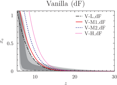
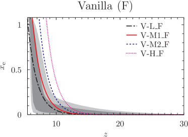
Figure 1: Evolution of the global ionized fraction in vanilla (“V”) reionization models with varying $f_{\gamma}$. Model specifications are shown in legends, and are listed in Table 1. (left) Vanilla models when “dF” scheme is used, and (right) vanilla models when “F” scheme is used. Throughout Figs 1 – 5, the ionized fraction is in terms of $x_{{\rm e}}\equiv n_{{\rm e}}/n_{{\rm H}}=1.079\,x$ which reaches the maximum value of 1.079, based on assuming that all helium atoms inside H II regions are singly ionized before the epoch of helium reionization occurring at $z\simeq 3.5$.

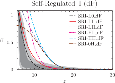
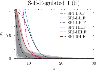
Figure 2: Evolution of the global ionized fraction in the model category “self-regulated I”. The model variance is specified by the set of $\left\{g_{\gamma}^{{\rm H}},\,g_{\gamma}^{{\rm L}}\right\}$ and are specified in legends, with the nomenclature “SI-$g_{\gamma}^{{\rm H}}$$g_{\gamma}^{{\rm L}}$” but $g_{\gamma}$’s with letters “0” for null, “L” for low and “H” for high. These models are listed in Table 1.

All models are described by simple ordinary differential equations (ODEs), and thus can be easily integrated with ODE solvers. We start numerical integration from $z=40$, when the contribution of any type of halos to reionization and heating is believed to be negligible. The initial value of $x$ is set to an arbitrarily small value, because the volume occupied by H II regions at $z=40$ must be negligible. Ionization rate equations to solve are not stiff, and we use a 4th-order, adaptive Runge-Kutta integrator with both the relative tolerance and the absolute tolerance of $x$ set to $10^{-5}$. For SRII, we need an extra effort to calculate $J_{{\rm LW}}(t)$ at any time $t$, because $J_{{\rm LW}}(t)$ regulates SFR inside MHs at $t$ via $x_{{\rm LW}}$ and impacts PPR (equations 12 and 13). Therefore, we calculate $x(t)$ and $J(t)$ at each incrementally increasing time step, by integrating equation 5 with equation 13 (or equation 12 if dF assumed) and using equations (14) and (16).

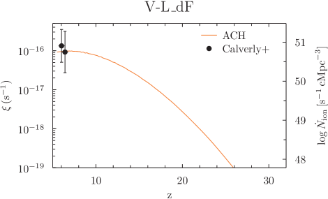
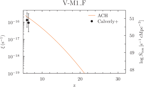
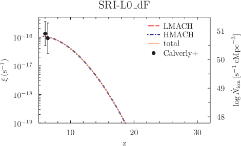
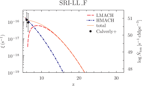
Figure 3: (top) Ionization rate and ionizing-photon emissivity ($\xi$ in equation 5 and $\dot{N}_{{\rm ion}}\equiv\xi n_{b,\,0}$) of PLD-favored vanilla and SRI models, compared to the $z=6.02$ and $z=6.42$ constraints by Calverley et al. (2011). Models are specified in the subtitle. For SRI cases, contributions by LMACHs (red, dashed) and HMACHs (blue, dot-dashed) are shown separately. The net quantities (orange, solid) are also plotted. Note that the constraint by Calverley et al. (2011) here are values of observed $\Gamma$ (section 2.3.1) translated into $\dot{N}_{{\rm ion}}$ based on a specific set of $\lambda_{{\rm mfp}}$ and the spectral hardness of H-ionizing photons: $\lambda_{{\rm mfp}}=10\,{\rm cMpc}$ and $\alpha_{{\rm s}}=\alpha_{{\rm b}}=2$ in equation (21) of Bolton & Haehnelt (2007).

Model	$g_{\gamma}^{{\rm H}}$	$g_{\gamma}^{{\rm L}}$	$M_{{\rm III}}$	$f_{{\rm esc}}^{{\rm M}}$	$J_{{\rm LW,th}}$	$z_{{\rm begin}}$	$z_{{\rm end}}$	$\Delta z_{3-97}$	$\tau_{{\rm es}}$	$\tau_{{\rm es}}(15-30)$	$\chi^{2}/\nu$
SRII-L0-100-e0.1-J0.05	0.8673	0	100	0.1	0.05	10.86	5.78	3.86	0.04801	3.45E-4	0.86
SRII-L0-100-e0.1-J0.10	0.8673	0	100	0.1	0.10	11.03	5.78	3.88	0.04850	6.18E-4	0.86
SRII-L0-100-e0.5-J0.05	0.8673	0	100	0.5	0.05	11.18	5.78	3.90	0.04983	1.72E-3	0.85
SRII-L0-100-e0.5-J0.10	0.8673	0	100	0.5	0.10	22.15	5.79	4.07	0.05226	3.08E-3	0.83
SRII-L0-100-e1.0-J0.05	0.8673	0	100	1.0	0.05	22.91	5.79	3.96	0.05210	3.44E-3	0.83
SRII-L0-100-e1.0-J0.10	0.8673	0	100	1.0	0.10	25.38	5.79	4.51	0.05696	6.17E-3	0.80
SRII-LL-100-e0.1-J0.05	0.8673	8.673	100	0.1	0.05	14.48	6.24	6.50	0.06168	3.75E-4	0.81
SRII-LL-100-e0.1-J0.10	0.8673	8.673	100	0.1	0.10	14.90	6.24	6.53	0.06199	6.37E-4	0.81
SRII-LL-100-e0.5-J0.05	0.8673	8.673	100	0.5	0.05	15.26	6.24	6.54	0.06284	1.44E-3	0.82
SRII-LL-100-e0.5-J0.10	0.8673	8.673	100	0.5	0.10	22.14	6.24	6.76	0.06446	2.78E-3	0.83
SRII-LL-100-e1.0-J0.05	0.8673	8.673	100	1.0	0.05	22.90	6.24	6.59	0.06432	2.79E-3	0.82
SRII-LL-100-e1.0-J0.10	0.8673	8.673	100	1.0	0.10	25.38	6.24	13.93	0.06762	5.50E-3	0.86
SRII-LH-100-e0.1-J0.05	0.8673	86.73	100	0.1	0.05	17.11	6.93	8.35	0.08832	1.01E-3	2.23
SRII-LH-100-e0.1-J0.10	0.8673	86.73	100	0.1	0.10	17.19	6.93	8.35	0.08847	1.15E-3	2.24
SRII-LH-100-e0.5-J0.05	0.8673	86.73	100	0.5	0.05	17.22	6.93	8.36	0.08895	1.60E-3	2.29
SRII-LH-100-e0.5-J0.10	0.8673	86.73	100	0.5	0.10	22.05	6.93	8.41	0.08973	2.37E-3	2.37
SRII-LH-100-e1.0-J0.05	0.8673	86.73	100	1.0	0.05	17.46	6.93	8.37	0.08976	2.35E-3	2.36
SRII-LH-100-e1.0-J0.10	0.8673	86.73	100	1.0	0.10	25.38	6.93	8.50	0.09135	3.91E-3	2.55
SRII-HL-100-e0.1-J0.05	6.938	8.673	100	0.1	0.05	14.62	8.27	4.82	0.07586	3.48E-4	1.17
SRII-HL-100-e0.1-J0.10	6.938	8.673	100	0.1	0.10	14.71	8.27	4.83	0.07610	5.70E-4	1.18
SRII-HL-100-e0.5-J0.05	6.938	8.673	100	0.5	0.05	14.79	8.27	4.84	0.07684	1.26E-3	1.20
SRII-HL-100-e0.5-J0.10	6.938	8.673	100	0.5	0.10	22.13	8.27	4.91	0.07807	2.40E-3	1.26
SRII-HL-100-e1.0-J0.05	6.938	8.673	100	1.0	0.05	15.35	8.27	4.86	0.07807	2.41E-3	1.25
SRII-HL-100-e1.0-J0.10	6.938	8.673	100	1.0	0.10	25.38	8.27	5.04	0.08057	4.70E-3	1.38
SRII-HH-100-e0.1-J0.05	6.938	86.73	100	0.1	0.05	17.12	8.79	6.74	0.09325	1.01E-3	2.96
SRII-HH-100-e0.1-J0.10	6.938	86.73	100	0.1	0.10	17.19	8.79	6.75	0.09339	1.16E-3	2.98
SRII-HH-100-e0.5-J0.05	6.938	86.73	100	0.5	0.05	17.22	8.79	6.75	0.09387	1.60E-3	3.04
SRII-HH-100-e0.5-J0.10	6.938	86.73	100	0.5	0.10	22.05	8.79	6.79	0.09464	2.35E-3	3.15
SRII-HH-100-e1.0-J0.05	6.938	86.73	100	1.0	0.05	17.43	8.79	6.76	0.09467	2.34E-3	3.14
SRII-HH-100-e1.0-J0.10	6.938	86.73	100	1.0	0.10	25.38	8.79	6.88	0.09622	3.87E-3	3.38
SRII-0H-100-e0.1-J0.05	0	86.73	100	0.1	0.05	17.11	4.10	10.12	0.08612	1.01E-3	1.99
SRII-0H-100-e0.1-J0.10	0	86.73	100	0.1	0.10	17.19	4.10	10.13	0.08627	1.15E-3	2.00
SRII-0H-100-e0.5-J0.05	0	86.73	100	0.5	0.05	17.22	4.10	10.13	0.08676	1.60E-3	2.04
SRII-0H-100-e0.5-J0.10	0	86.73	100	0.5	0.10	22.05	4.10	10.18	0.08754	2.37E-3	2.12
SRII-0H-100-e1.0-J0.05	0	86.73	100	1.0	0.05	17.46	4.10	10.15	0.08756	2.35E-3	2.11
SRII-0H-100-e1.0-J0.10	0	86.73	100	1.0	0.10	25.38	4.10	10.27	0.08916	3.92E-3	2.27

Table 2: Model parameters and resulting characteristics of SRII, with $M_{{\rm III}}=100\,M_{\odot}$. Notes: In the table, $M_{{\rm III}}$ and $J_{{\rm LW,\,th}}$ are in units of $M_{\odot}$ and $10^{-21}\,{\rm erg\,s^{-1}\,cm^{-2}\,Hz^{-1}\,sr^{-1}}$, respectively. Highlighted in grey are those that fit the observed $C_{l}^{{\rm EE}}$ of the PLD best.

The vanilla model shows a smooth and monotonic evolution of $x$ (Fig. 1). The monotonic behavior of $x(t)$ is easily explained by the fact that $\xi$ is proportional to the monotonically increasing $f_{{\rm coll}}$ (F scenario) or $df_{{\rm coll}}/dt$ (dF scenario). This characteristic makes $\tau_{{\rm es}}$ and $z_{{\rm end}}$ tightly correlated, and thus lacks the “leverage” to accommodate reionization scenarios that are different in $x(z)$ but degenerate in $\tau_{{\rm es}}$ and $z_{{\rm end}}$, as long as one type of star formation scenarios are chosen from F or dF. One can of course make a somewhat more sophisticated variant of this model by e.g. allowing multiple species of halos with different $f_{\gamma}$’s (mixture of Pop II and Pop III stars Furlanetto 2006). Nevertheless, due to the lack of any self-regulation, the resulting reionization histories of such variants would still remain similar to the original vanilla model. The duration of reionization is in general more extended in the dF scenario than the F scenario. This is due to the fact that $df_{{\rm coll}}/dt$ grows more slowly than $f_{{\rm coll}}$. Therefore, for given $z_{{\rm end}}$, the dF scenario produces larger $\tau_{{\rm es}}$ than the F scenario. This tendency is clearly presented in figure 1 and Table 1.

Model	$g_{\gamma}^{{\rm H}}$	$g_{\gamma}^{{\rm L}}$	$M_{{\rm III}}$	$f_{{\rm esc}}^{{\rm M}}$	$J_{{\rm LW,th}}$	$z_{{\rm begin}}$	$z_{{\rm end}}$	$\Delta z_{3-97}$	$\tau_{{\rm es}}$	$\tau_{{\rm es}}(15-30)$	$\chi^{2}/\nu$
SRII-L0-300-e0.1-J0.05	0.8673	0	300	0.1	0.05	10.89	5.78	3.86	0.04817	4.50E-4	0.86
SRII-L0-300-e0.1-J0.10	0.8673	0	300	0.1	0.10	11.10	5.78	3.89	0.04875	7.75E-4	0.86
SRII-L0-300-e0.5-J0.05	0.8673	0	300	0.5	0.05	11.45	5.78	3.92	0.05063	2.29E-3	0.84
SRII-L0-300-e0.5-J0.10	0.8673	0	300	0.5	0.10	23.26	5.79	4.14	0.05350	3.88E-3	0.82
SRII-L0-300-e1.0-J0.05	0.8673	0	300	1.0	0.05	23.50	5.79	4.02	0.05365	4.50E-3	0.82
SRII-L0-300-e1.0-J0.10	0.8673	0	300	1.0	0.10	27.15	5.79	15.28	0.05960	7.79E-3	0.80
SRII-LL-300-e0.1-J0.05	0.8673	8.673	300	0.1	0.05	14.51	6.24	6.50	0.06177	4.49E-4	0.81
SRII-LL-300-e0.1-J0.10	0.8673	8.673	300	0.1	0.10	15.26	6.24	6.54	0.06215	7.73E-4	0.82
SRII-LL-300-e0.5-J0.05	0.8673	8.673	300	0.5	0.05	20.00	6.24	6.55	0.06330	1.83E-3	0.82
SRII-LL-300-e0.5-J0.10	0.8673	8.673	300	0.5	0.10	23.26	6.24	6.86	0.06528	3.45E-3	0.83
SRII-LL-300-e1.0-J0.05	0.8673	8.673	300	1.0	0.05	23.50	6.24	6.65	0.06527	3.57E-3	0.83
SRII-LL-300-e1.0-J0.10	0.8673	8.673	300	1.0	0.10	27.15	6.24	14.77	0.06944	6.96E-3	0.88
SRII-LH-300-e0.1-J0.05	0.8673	86.73	300	0.1	0.05	17.12	6.93	8.35	0.08836	1.04E-3	2.23
SRII-LH-300-e0.1-J0.10	0.8673	86.73	300	0.1	0.10	17.21	6.93	8.36	0.08856	1.23E-3	2.25
SRII-LH-300-e0.5-J0.05	0.8673	86.73	300	0.5	0.05	17.26	6.93	8.36	0.08917	1.77E-3	2.30
SRII-LH-300-e0.5-J0.10	0.8673	86.73	300	0.5	0.10	23.22	6.93	8.42	0.09022	2.78E-3	2.41
SRII-LH-300-e1.0-J0.05	0.8673	86.73	300	1.0	0.05	17.69	6.93	8.38	0.09024	2.74E-3	2.40
SRII-LH-300-e1.0-J0.10	0.8673	86.73	300	1.0	0.10	27.15	6.93	8.54	0.09235	4.76E-3	2.64
SRII-HL-300-e0.1-J0.05	6.938	8.673	300	0.1	0.05	14.63	8.27	4.82	0.07594	4.10E-4	1.17
SRII-HL-300-e0.1-J0.10	6.938	8.673	300	0.1	0.10	14.75	8.27	4.83	0.07623	6.85E-4	1.18
SRII-HL-300-e0.5-J0.05	6.938	8.673	300	0.5	0.05	14.91	8.27	4.85	0.07722	1.58E-3	1.22
SRII-HL-300-e0.5-J0.10	6.938	8.673	300	0.5	0.10	23.26	8.27	4.93	0.07875	2.97E-3	1.28
SRII-HL-300-e1.0-J0.05	6.938	8.673	300	1.0	0.05	23.50	8.27	4.88	0.07880	3.01E-3	1.28
SRII-HL-300-e1.0-J0.10	6.938	8.673	300	1.0	0.10	27.15	8.27	5.12	0.08198	5.90E-3	1.45
SRII-HH-300-e0.1-J0.05	6.938	86.73	300	0.1	0.05	17.12	8.79	6.74	0.09329	1.05E-3	2.97
SRII-HH-300-e0.1-J0.10	6.938	86.73	300	0.1	0.10	17.20	8.79	6.75	0.09349	1.24E-3	2.99
SRII-HH-300-e0.5-J0.05	6.938	86.73	300	0.5	0.05	17.27	8.79	6.75	0.09411	1.78E-3	3.06
SRII-HH-300-e0.5-J0.10	6.938	86.73	300	0.5	0.10	23.22	8.79	6.81	0.09513	2.77E-3	3.21
SRII-HH-300-e1.0-J0.05	6.938	86.73	300	1.0	0.05	17.58	8.79	6.77	0.09512	2.69E-3	3.19
SRII-HH-300-e1.0-J0.10	6.938	86.73	300	1.0	0.10	27.15	8.79	6.91	0.09721	4.70E-3	3.50
SRII-0H-300-e0.1-J0.05	0	86.73	300	0.1	0.05	17.12	4.10	10.12	0.08617	1.04E-3	1.99
SRII-0H-300-e0.1-J0.10	0	86.73	300	0.1	0.10	17.21	4.10	10.13	0.08637	1.24E-3	2.01
SRII-0H-300-e0.5-J0.05	0	86.73	300	0.5	0.05	17.27	4.10	10.13	0.08698	1.78E-3	2.06
SRII-0H-300-e0.5-J0.10	0	86.73	300	0.5	0.10	23.22	4.10	10.19	0.08803	2.79E-3	2.16
SRII-0H-300-e1.0-J0.05	0	86.73	300	1.0	0.05	17.69	4.10	10.15	0.08802	2.71E-3	2.14
SRII-0H-300-e1.0-J0.10	0	86.73	300	1.0	0.10	27.15	4.10	10.31	0.09016	4.77E-3	2.36

Table 3: Model parameters and resulting characteristics of SRII, with $M_{{\rm III}}=300\,M_{\odot}$. Notes: The unit convention is the same as in Table 2. Highlighted in grey are those that fit the observed $C_{l}^{{\rm EE}}$ of the PLD best.

The SRI model adds a little more complexity to the characteristics compared to the vanilla model (Fig. 2). Due to the existence of self-regulation, the SRI is expected to have more extended reionization histories than the vanilla model. This has indeed been shown to be the case for a consistent halo-selection criterion for HMACH and LMACH (Iliev et al. 2007). However, one subtlety in our modelling scheme complicates such an expectation. Because we use a constant mass criterion in SRI, while a constant temperature criterion in the vanilla model, we find that in some cases the duration of SRI models can be shorter than that of vanilla models. Had we used the same halo selection criterion, SRI models would have larger $\Delta z$ than vanilla models, which we actually tested and confirmed. Aside from this complication which is not essential, the general trend is that (1) the larger the value of $g_{\gamma}^{{\rm L}}/g_{\gamma}^{{\rm H}}$ is, the larger the duration of reionization becomes and (2) addition of LMACHs to HMACH-only scenarios extends the duration of reionization. Also, cases with very large $g_{\gamma}^{{\rm L}}/g_{\gamma}^{{\rm H}}$ (e.g. SRI-0H_F case in Fig. 2) slows down reionization significantly at the end of reionization, producing histories as symmetric as the tangent-hyperbolic model that has been used extensively in the analysis of the CMB data. It is easy to understand this behavior: $g_{\gamma}^{{\rm L}}/g_{\gamma}^{{\rm H}}$ is a rough measure of the relative contribution of LMACH to reionization to that of HMACH, and the self-regulation becomes stronger as $x$ becomes larger. One very extreme case is SRI-0H_dF, which never finishes reionization due to a strong self-regulation. The trend that $\Delta z$ is larger in the dF scenario than the F scenario is the same as in the vanilla model. The general trend of the vanilla and SRI models can also be seen in Figure 3 in terms of $\xi$.

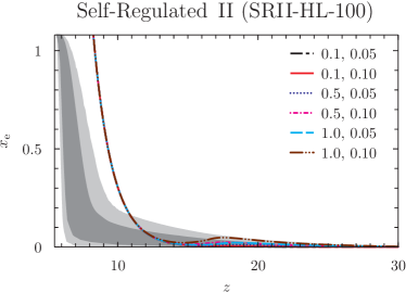
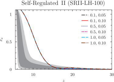
Figure 4: Evolution of the global ionized fraction in the model category “self-regulated II”, with $M_{{\rm III}}=100\,M_{\odot}$ per MH. Each panel corresponds to varying sets of $\{g_{\gamma}^{{\rm H}},\,g_{\gamma}^{{\rm L}},\,M_{{\rm III}}\}$, denoted in the format “SRII-$g_{\gamma}^{{\rm H}}g_{\gamma}^{{\rm L}}$-$M_{{\rm III}}/M_{\odot}$”. The letters “0”, “L” and “H” denote “null”, “low” and “high” values of $g_{\gamma}$, respectively, in relative sense (listed in Table 1). In all panels, the set of $f_{{\rm esc}}^{{\rm M}}$ and $J_{{\rm LW,th}}$ (in units of $10^{-21}\,{\rm erg\,s^{-1}\,cm^{-2}\,Hz^{-1}\,sr^{-1}}$) are specified as legends: {0.1, 0.05}, black dot-long-dashed; {0.1, 0.10}, red solid; {0.5, 0.05}, blue dotted; {0.5, 0.10}, magenta dot-short-dashed; {1.0, 0.05}, cyan dashed; {1.0, 0.10}, brown dot-dot-dashed.

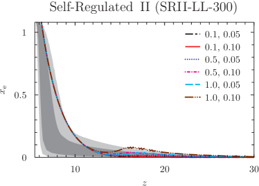
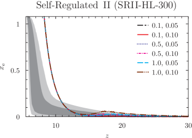
Figure 5: Same as Fig 4 but with $M_{{\rm III}}=300\,M_{\odot}$. Each panel corresponds varying $f_{\gamma}^{{\rm H}}$ and $M_{{\rm III}}$ as specified in the title. In all panels, the set of $f_{{\rm esc}}^{{\rm M}}$ and $J_{{\rm LW,th}}$ (in units of $10^{-21}\,{\rm erg\,s^{-1}\,cm^{-2}\,Hz^{-1}\,sr^{-1}}$) are specified as legends using the same line convention as Figure 4.

The SRII model has features richer than the vanilla and the SRI models (Figures 4 and 5). The most notable feature is the existence of the early, extended and slowly-increasing phase in $x$. This is due to the self-regulation of star formation, even stronger than that in the SRI model, which takes place inside MHs. The star formation inside MHs are mainly regulated by the LW background $J_{{\rm LW}}$, which quickly builds up to reach $J_{{\rm LW,\,th}}$. Continuum photons below the Lyman limit and emitted at redshift $z$ travels a cosmological distance ($\sim 100\{(1+z)/21\}^{-0.5}\,$cMpc), in contrast to the hydrogen-ionizing UV photons that travel up to the ionization front and then absorbed. Therefore, any newly forming MHs will be under the influence of LW background long before being exposed to the ionizing photons, and any pre-ionized region would have been under the over-critical LW intensity ($J_{{\rm LW}}>J_{{\rm LW,\,th}}$). We find that this is indeed the case: when tested with $\max(x_{{\rm LW}},\,x)$ replaced by $x_{{\rm LW}}$ in equation (13), the resulting $x(z)$ was not affected.

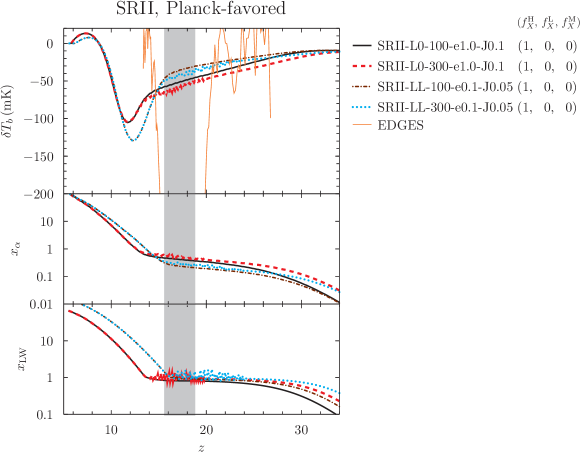
Figure 11: 21 cm backgrounds (top), the Ly$\alpha$ coupling coefficients (middle) and $x_{{\rm LW}}$ ($=J_{{\rm LW}}/J_{{\rm LW,th}}$) of models that fit PLD best (those marked by arrows in Fig 7), selected from SRII. In order to avoid crowdedness, we take only 4 models among those that match PLD best. Regardless of the difference in values of $J_{{\rm LW,th}}$, MHs self-regulate star formation such that $x_{{\rm LW}}\simeq 1$ is maintained after $J_{{\rm LW}}$ reaches $\sim J_{{\rm LW,th}}$. This tendency continues until ACHs take over to dominate in contributing to $J_{{\rm LW}}$ by generating stars without being hindered by the LW feedback. At the same time, this self-regulation limits $x_{\alpha}\lesssim 0.5$, with additive dependence on $f_{{\rm esc}}^{{\rm M}}$.

Another notable feature of SRII is that, in some cases where the contribution of ionizing photons by MHs is as significant as to drive $x$ beyond $\gtrsim 10\%$, there exists a phase where $x$ decreases in time. This is mainly due to the fact that (1) the LW feedback renders $J_{{\rm LW}}\simeq J_{{\rm LW\,th}}$ when MHs dominate as the main radiation sources (Fig. 11) and (2) the large difference in the number of soft-UV ($h\nu=\sim 11-13.6\,{\rm eV}$) photons per ionizing photon of Pop II and Pop III stars (see the detail in Section 2.4) and (3) the drop of $f_{{\rm esc}}$ from MH values ($f_{{\rm esc}}\sim 1$) to ACHS ($f_{{\rm esc}}\sim 0.2$). Then, as LMACHS (assumed to host Pop III stars) and HMACHs (assumed to host Pop II stars) start to generate soft-UV photons to make up $J_{{\rm LW}}$ near $J_{{\rm LW\,th}}$, which is achieved at the expense of ACHs’ putting out much less amount of ionizing photons than minihalos (assumed to host Pop III stars), the IGM gains a chance to recombine faster than ionization (Fig. 6: see dips in $\xi$). In practice, however, this recombination is slight and not as dramatic as the “double reionization” that has been suggested by Cen (2003). Given the same set of $\left\{g_{\gamma}^{{\rm H}},\,g_{\gamma}^{{\rm L}}\right\}$ as in SRI, the SRII model has $z_{{\rm end}}$ that is practically identical to that of SRI while $\tau_{{\rm es}}$ and $\Delta z$ that are both boosted from those of SRI (Tables 1 – 3). This is simply due to the existence of additional photon sources, or MH stars, that ionize the IGM only to a limited extent ($x\lesssim 15\,\%$ at most under our parameter range but may be increased if $M_{{\rm III}}$ and $J_{{\rm LW,th}}$ are pushed to higher values) such that $z_{{\rm end}}$ is not much affected but can increase $\tau_{{\rm es}}$ and extend the duration of reionization substantially by strongly regulated ionization history.

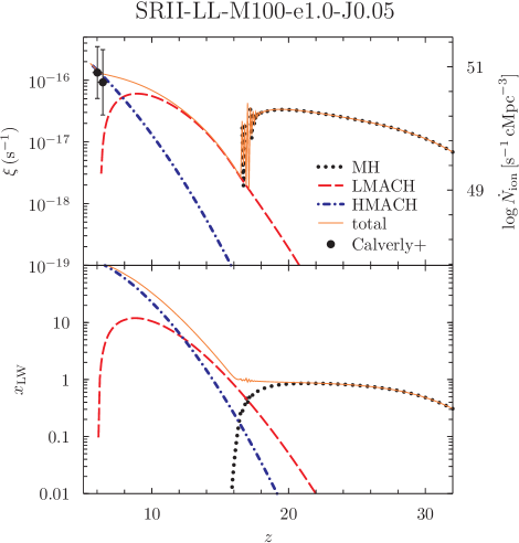
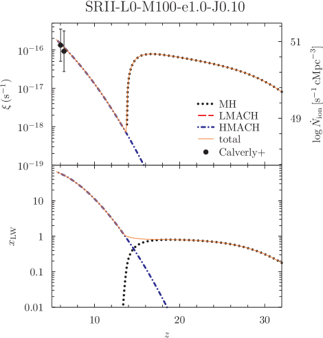
Figure 6: (top) Same as Figure 3, and (bottom) the Lyman-Werner band intensity in terms of $x_{{\rm LW}}\equiv J_{{\rm LW}}/J_{{\rm LW,\,th}}$ (equation 14), for two selected cases among PLD-favored SRII models. Line convention is identical to Figure 3, and contributions by MHs (black, dotted) are shown in addition.

3.2 Comparison with CMB observations

The 2018 PLD provides, among improvements from the 2015 data, so far the most precise measurement of the large-scale CMB polarization anisotropy. The large-scale E-mode auto-correlation angular power spectrum, $C_{l}^{{\rm EE}}$, is strongly affected by the history of reionization. The quadrupole moment of the CMB anisotropy generates linear polarization after Thomson scattering from the viewpoint of an electron, and the polarization signal is observed after being modulated by the relevant wave-modes, resulting in affecting $C_{l}^{{\rm EE}}$ mostly in the low-$l$ ($\lesssim 20$) regime (Hu & White 1997; Haiman & Knox 1999; Dodelson 2003).

The extended high-redshift ($z\gtrsim 15$) ionization tail predicted by Ahn et al. (2012) and SRII models here has been advocated by Miranda et al. (2017) and Heinrich & Hu (2018), based on their principal component analysis (PCA) of the Planck 2015 $C_{l}^{{\rm EE}}$ data observed through the Low-Frequency Instrument (LFI). They claimed that a specific SRII model with a substantial high-redshift tail, corresponding roughly to L2M1J2 case of Ahn et al. (2012), was favored over the vanilla model at $\sim 1\sigma$ level. Later, Millea & Bouchet (2018) used both the LFI and the HFI (proprietary at the time) data, with a well-handled physicality ($x>0$) prior, to claim against too much contribution from the $z\gtrsim 15$ epoch. They constrained the optical depth from $15\leq z\leq 30$, or $\tau(15,30)$, to $\tau(15,30)<0.015$ at $2\sigma$ level. The Planck 2018 analysis based only on the low-$l$ E-mode polarization further reduces this value to $\tau(15,30)<0.007$ at $2\sigma$ level and $\tau_{{\rm es}}=0.0504_{-0.0079}^{+0.0050}$ at $1\sigma$ level (Planck Collaboration et al. 2018).

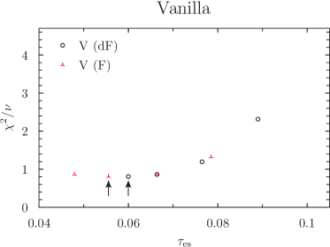
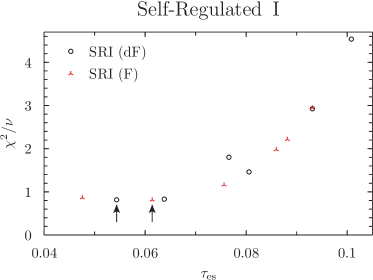
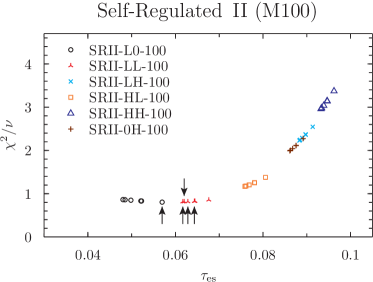
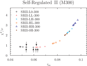
Figure 7: $\chi^{2}/\nu$ of the E-mode power spectrum $D_{l}^{{\rm EE}}$ of each model with respect to the Planck 2018 Legacy Data. In each panel, plotted points are grouped in sub-categories specified by legends, and arrows point to the minimum-$\chi^{2}/\nu$ cases in each panel. Models marked by arrows correspond to those highlighted in Tables 1 – 3.

In light of the constraints described above, we compare our model $x(z)$’s from Section 3.1 to PLD. The main purpose of this task is to (1) understand whether any class of our models are preferred by observation and (2) whether the degeneracy of models in $\tau_{{\rm es}}$ and $z_{{\rm ov}}$ can be broken. For example, Ahn et al. (2012) showed that SRII models with an extended tail in $x(z)$ could be distinguished from the vanilla- or SRI-type models, even when the models have the same $\tau_{{\rm es}}$ (=0.085) and $z_{{\rm ov}}$ (=6.8). The pictorial comparison of $x(z)$ to the Planck constraint ($1\sigma$ and $2\sigma$ constraints shown in shaded regions) is shown in Figs. 1 – 5. We test the relative goodness of several selected models by calculating the reduced chi square,

$$\chi^{2}/\nu=\frac{1}{29}\sum_{l=2}^{30}\frac{(D_{l}^{{\rm EE}}-\tilde{D}_{l}^{{\rm EE}})^{2}}{\sigma_{l}^{2}},$$ (31)

where $D_{l}^{{\rm EE}}\equiv l(l+1)C_{l}^{{\rm EE}}/(2\pi)$ and $\tilde{D}_{l}^{{\rm EE}}\equiv l(l+1)\tilde{C}_{l}^{{\rm EE}}/(2\pi)$ are the E-mode power spectrums corresponding to a model $x(z)$ and PLD respectively, and $\sigma_{l}$ is the standard deviation of $\tilde{D}_{l}^{{\rm EE}}$ due to the cosmic variance and the noise. $C_{l}^{{\rm EE}}\equiv\left\langle\left|a_{lm}^{{\rm E}}\right|^{2}\right\rangle$ for given $l$ averaged over $m=[-l,\,l]$, with the spherical-harmonics decomposition of the E-mode anisotropy $E(\theta,\,\phi)=\sum_{lm}a_{lm}^{{\rm E}}Y_{lm}(\theta,\,\phi)$. In calculating $D_{l}^{{\rm EE}}$, we use a version of the Boltzmann solver CAMB that was modified to allow a generic shape of $x(z)$ (Mortonson & Hu 2008, downloadable from http://background.uchicago.edu/camb_rpc/). For the base cosmology, we use the best-fit parameter set of PLD. While this is not a full likelihood analysis including other data products such as the temperature anisotropy, the value of $\chi^{2}/\nu$ from equation (31) can indicate the relative goodness of models because the impact of reionization histories is the strongest in the E-mode (see e.g. an identical approach by Qin et al. 2020b). E-mode power spectrums of selected models against the PLD are plotted in Fig. 8.

It is interesting to note that the constraint on reionization by the Planck observation provides a good match to the observed $\Gamma$ (section 2.3.1). If the observed $\Gamma$ (e.g. Calverley et al. 2011) is translated into $\dot{N}_{{\rm ion}}$ with a reasonable set of physical parameters ($\lambda_{{\rm mfp}}=10\,{\rm cMpc}$: the IGM mean free path to H-ionizing photons at $z\simeq 6$, and $\alpha_{{\rm s}}=\alpha_{{\rm b}}=2$: the spectral hardness of H-ionizing photons in equation (21) of Bolton & Haehnelt 2007), PLD-favored models have a good agreement with the observed $\Gamma$ at $z\simeq 6$ (Figures 3 and 6). This consistency between the two independent observations, even though uncertainties are large, is encouraging.

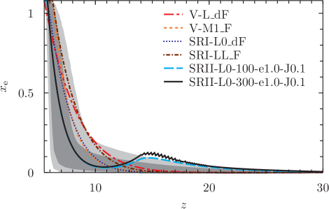
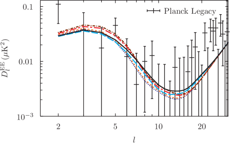
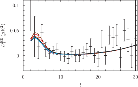
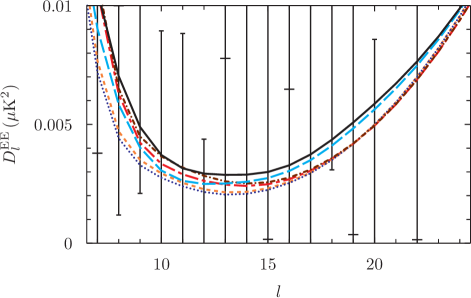
Figure 8: Low-multipole E-mode auto-correlation power spectrums predicted by models (lines with model specification on the top-left panel) with smallest $\chi^{2}/\nu$ and that of PLD (points with $1\sigma$ error bar). We select only two models with smallest $\chi^{2}/\nu$ from SRII models, to avoid crowdedness of lines. CMB lensing is considered in all cases, even though the net effect in this range of $l$ is weak. Different plotting schemes (top-right: logarithmic; bottom-left: linear; bottom-right: linear-zoomed) are used. SRII models with the high-$z$ ionization tail achieve larger values of $D_{l}^{{\rm EE}}$ for $14\lesssim l\lesssim 24$ than vanilla and SRI models, even though all the models plotted here share about a single value of $\tau_{{\rm es}}$ ($\simeq 0.06$).

We now claim that some SRII models with substantial high-redshift tails are still among those highly favored by PLD. Because $\chi^{2}/\nu$ is a measure of the goodness of a fit, we can use the value of $\chi^{2}/\nu$ to find the PLD-favored models. We indeed find many models can explain the PLD low-$l$ $C_{l}^{{\rm EE}}$ fairly well even though the variance in $\tau_{{\rm es}}$ of such models is substantial. Models that fit the PLD $C_{l\leq 30}^{{\rm EE}}$ best are marked by arrows in Fig. 7 and highlighted in Tables 1 – 3: all these models have almost the same likelihood with $\chi^{2}/\nu=0.80-0.82$, but with a substantial spread on $\tau_{{\rm es}}$ with $\tau_{{\rm es}}\simeq[0.0544,\,0.0643]$. If allowance is extended to models with $\chi^{2}/\nu\leq 1$, then the allowed optical depth becomes $\tau_{{\rm es}}\simeq[0.044,\,0.072]$. This indicates that some of our SRII models are still well within the PLD constraint and as much favored as those models without high-redshift ionization tails. As seen in Tables 1 – 3, the most favored model with the least $\chi^{2}/\nu$, $\chi^{2}/\nu$=0.80, are indeed SRII-L0-100-e1.0-J0.1 and SRII-L0-300-e1.0-J0.1, which have a substantial high-redshift tail that reaches maximum $x=0.12$ at $z=13.6$ and $x=0.15$ at $z=13.6$, respectively. Such tails contribute to $\tau_{{\rm es}}(15-30)$ substantially: $\tau_{{\rm es}}(15-30)=0.0063$ and 0.0078 for SRII-L0-100-e1.0-J0.1 and SRII-L0-300-e1.0-J0.1, respectively. We also note that these maximum-likelihood models are clustered around $\tau_{{\rm es}}=0.06$, substantially different from the inferred value $\tau_{{\rm es}}=0.0504$ by PLD-$C_{l\leq 30}^{{\rm EE}}$. The reason why such a difference occurs is unclear; this is nevertheless a very important issue and a further investigation is warranted.

The model with the strongest ionization tail of all, SRII-L0-300-e1.0-J0.1, is worthy of a close attention. Compared to the 2$\sigma$ constraint of PLD, $\tau_{{\rm es}}(15-30)<0.007$, SRII-L0-300-e1.0-J0.1 actually violates this constraint with $\tau_{{\rm es}}(15-30)=0.0078$ but is still the best-fit (to PLD $C_{l\leq 30}^{{\rm EE}}$) of all the models we tested. This model also has $\tau_{{\rm es}}=0.0596$, which is about $2\sigma$ away from the E-mode only best-fit estimate by PLD, $\tau_{{\rm es}}=0.0504$. If we do not consider other CMB observables and assume a flat prior, we can conclude that this model is as good as or just slightly better than other tail-less models with $\chi^{2}/\nu=0.81-0.82$. It is interesting to see that there exists a weak tension between $\tau_{{\rm es}}$’s estimated by the low-$l$ E-mode polarization and the CMB lensing: the low-$l$ E-mode data of PLD prefers such a low $\tau_{{\rm es}}\,(=0.0504_{-0.0079}^{+0.0050})$, while the CMB lensing of PLD prefers higher $\tau_{{\rm es}}$ at around $\tau_{{\rm es}}\simeq 0.08$ (Planck Collaboration et al. 2018). This tendency of the CMB lensing favoring large values of $\tau_{{\rm es}}$, even though the uncertainty is large, is in par with favoring two-stage reionization models with substantial ionization tails. Our findings are in slight disagreement with the PLD constraint that was constructed using non-parametric Bayesian inference. Based on our forward modelling and goodness-of-fit approach, we argue that a family of models with a substantial high-redshift ionization tail reaching $x_{{\rm max}}\sim 0.12$ are still very strong contenders at the moment just as those tail-less models.

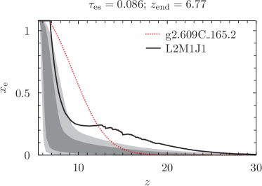
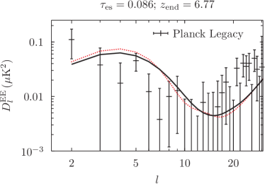
Figure 9: Breaking degeneracy in $\tau_{{\rm es}}$ and $z_{{\rm end}}$ by E-mode polarization observation. (left) $x(z)$’s of two selected reionization models from Ahn et al. (2012), sharing the same $\tau_{{\rm es}}$ ($=0.086$) and $z_{{\rm end}}$ (=6.77) but are grossly different in $x(z)$ with (L2M1J1: black, solid) and without substantial high-$z$ ionization tail (g2.609C_165.2: red, dotted), are plotted against the PLD constraint (grey shades). (right) E-mode polarization power spectrums of the two models, against the PLD data (data points with error bar), showing difference at $l\lesssim 24$.

Will there be a chance to probe a high-redshift ionization tail in the future? The high-redshift tail tends to boost $C_{l}^{{\rm EE}}$ at $14\lesssim l\lesssim 24$ (e.g. Ahn et al. 2012; Miranda et al. 2017): SRII models in Fig. 8 produce $C_{14\leq l\leq 24}^{{\rm EE}}$ larger than that of the rest of models, and especially SRII-L0-300-e1.0-J0.1 has the strongest $C_{l}^{{\rm EE}}$ at $8\leq l\leq 24$. In principle, models degenerate in $\tau_{{\rm es}}$ can have different $C_{l<30}^{{\rm EE}}$’s due to the variance in $x(z)$. Ahn et al. (2012), using a principal component analysis (PCA), had indeed predicted that high-precision CMB observation could break the degeneracy in $\tau_{{\rm es}}$ and probe (or disprove) the existence of the high-redshift ionization tail. We stress this point again through Fig. 9, showing two models from Ahn et al. (2012) that are degenerate both in $\tau_{{\rm es}}$ and $z_{{\rm end}}$ but are clearly different in $x(z)$, especially in the existence of the high-$z$ ionization tail, and in the resulting $C_{l}^{{\rm EE}}$. From Figures 8 and 9, we observe that the boost of $C_{14\leq l\leq 24}^{{\rm EE}}$ in two-stage reionization models with the high-$z$ ionization tail against those tail-less models is a universal effect. As seen in Fig. 7, the relation between $\tau_{{\rm es}}$ and $\chi^{2}/\nu$ is not exactly monotonic but instead there exists some scatter in $\chi^{2}/\nu$ for the same $\tau_{{\rm es}}$ and vice versa. Such a scatter increases as $\tau_{{\rm es}}$ increases, which is due to the increased freedom in constructing $x(z)$ for given $\tau_{{\rm es}}$. However, because the PLD E-mode power spectrum prefers such a low $\tau_{{\rm es}}$, as of now the leverage of having a pronounced tail has somewhat diminished from that prediction. Nevertheless, it is possible that observation by a more accurate apparatus might find preference for higher $\tau_{{\rm es}}$ than Planck that are still hampered by the large noise in measuring the polarization anisotropy. Therefore, we need a better apparatus than Planck to (1) see whether $\tau_{{\rm es}}$ could get larger than the estimate by PLD to allow more pronounced two-stage reionization models and (2) break the model degeneracy in $\tau_{{\rm es}}$ better than Planck to probe the ionization tail even when the tail is weak.

We also briefly describe another type of constraint from CMB observations. The kinetic Sunyaev-Zel’dovich effect can arise from the peculiar motion of H II bubbles during EoR and can affect the small-scale ($l\sim$ a few thousands) temperature anisotropy power spectrum $C_{l}^{{\rm TT}}$. Measurement of $C_{l}^{{\rm TT}}$ by the South Pole Telescope, especially $C_{l=3000}^{{\rm TT}}$, (SPT: Reichardt et al. 2012) was used by Zahn et al. (2012) to constrain the duration of reionization $\Delta z\equiv z(x=0.25)-z(x=0.99)$ to $\Delta z<4-7$ at $2\sigma$ level (depending on the assumed correlation between the thermal Sunyaev-Zel’dovich effect and the cosmic infrared background; see also the similar assessment by Mesinger et al. 2012 and Battaglia et al. 2013). Without MH stars, reionization occurs always in a patchy way and thus any addition of electrons, or equivalently extension of $\Delta z$, increases $C_{l=3000}^{{\rm TT}}$ monotonically, as was assumed in Zahn et al. (2012), Mesinger et al. (2012) and Battaglia et al. (2013). However, Park et al. (2013) re-addressed this issue with a variety of reionization scenarios including the SRII-type, and found that the added duration of reionization beyond this limit could still be accommodated by the measured $C_{l=3000}^{{\rm TT}}$. As claimed in Park et al. (2013), H II regions by MHs are distributed almost uniformly (Ahn et al. 2012) and thus the increase in $\Delta z$ in SRII models does not guarantee an increase in $C_{l=3000}^{{\rm TT}}$. Therefore, the largeness of $\Delta z_{3-97}\equiv z(0.03)-z(x=0.97)$ of many SRII models (see e.g. those highlighted in Tables 2 and 3) should not be considered as a violation of such a constraint. Instead, constraining $\Delta z$ using the small-scale $C_{l}^{{\rm TT}}$ should be restricted to only a limited set of models without MHs.

3.3 21 cm background and comparison with EDGES observation

The main variants determining $\delta T_{b}$ are the X-ray heating efficiency and the Ly$\alpha$ intensity, which determine $T_{{\rm K}}$ and $x_{\alpha}$, respectively. The X-ray efficiency is not a direct product of the stellar radiation and is thus the main cause of the uncertainty in $\delta T_{b}$. The Ly$\alpha$ intensity, on the other hand, is almost solely determined by the stellar radiation and is closely related to the ionizing PPR and the SED. We do not consider the creation of Ly$\alpha$ photons due to the excitation of H atoms by the X-ray-induced electrons, which is a good approximation unless the X-ray efficiency is extremely high ($f_{x}\gg 1$ with $f_{x}$ in equation 32). For the X-ray efficiency, we use the common parameter $f_{X}$ (Furlanetto 2006; Mirocha 2014), defined as the fudge parameter connecting the comoving X-ray luminosity density $\mathcal{L}_{\nu}$ ($=h\nu\mathcal{N}_{\nu}$; in ${\rm erg\,{\rm s^{-1}\,Hz^{-1}\,cMpc^{-3}}})$ to SFRD (Section 2.1):

$$f_{X}=\frac{\mathcal{L}_{\nu}}{c_{X}{\rm SFRD}},$$ (32)

where the additional proportionality coefficient $c_{X}$ is fixed to $c_{X}=3.4\times 10^{40}\,{\rm erg\,s^{-1}\,(M_{\odot}\,yr^{-1})}$, an extrapolation of the 2–10 keV relation between $\mathcal{L}_{\nu}$ and SFRD (or equivalently between $L_{\nu}$ and SFR on average galaxies) by Grimm et al. (2003) to $h\nu\geq 0.2\,{\rm keV}$. Here, we limit $\mathcal{L}_{\nu}$ to the energy range $h\nu=[0.2,\,30]\,{\rm keV}$ and a power-law SED $\mathcal{L}_{\nu}\propto\nu^{-1.5}$. For the Ly$\alpha$ intensity and the LW intensity, we take a simple distinction between Pop II and Pop III stars. Pop III stars are assumed to have $N_{{\rm ion}}=50000$, $N_{\alpha L}=4800$ and $N_{\beta L}=2130$, where $N_{\alpha L}$ and $N_{\beta L}$ are the number of photons emitted by a stellar baryon during the stellar lifetime in the energy range from Ly$\alpha$ to LL and from Ly$\beta$ to LL, respectively. Pop II stars are assumed to have $N_{{\rm ion}}=6000$, $N_{\alpha L}=9690$ and $N_{\beta L}=3170$. This makes $N_{\alpha L}/N_{{\rm ion}}$ and $N_{\beta L}/N_{{\rm ion}}$ of Pop III stars about an order of magnitude smaller than those of Pop II stars, respectively. $N_{\alpha L}/N_{{\rm ion}}$ and $N_{\beta L}/N_{{\rm ion}}$ strongly affect $J_{{\rm LW}}$ (equation 16) and $N_{\alpha}$ (equation 24) for given PPR. We use the following SED conventions for each category of models:

• Vanilla model: Pop II SED

• SRI model: Pop III SED for LMACH; Pop II SED for HMACH

• SRII model: Pop III SED for LMACH and MH; Pop II SED for HMACH

The claimed detection of $\sim 500\,{\rm mK}$ absorption dip around $\nu\simeq 78\,{\rm MHz}$ by the EDGES has been a matter of debate, mainly due to the fact that it is impossible to explain such a large amplitude in the standard $\Lambda$CDM framework, if the background after a successful foreground removal is composed only of the CMB and the 21cm background. In the $\Lambda$CDM universe the kinetic temperature of the IGM is limited to the adiabatically cooled value ($T_{{\rm K}}\sim 10.2\,{\rm K}[(1+z)/21]^{2}$), and even at the maximum Ly$\alpha$ coupling is limited to $\delta T_{b}\lesssim 200\,{\rm mK}$. Another difficulty faced by the EDGES result is the existence of a peculiar spectral shape in $\delta T_{b}$, a flat trough of $\delta T_{b}$ from $\nu=72$ to $85\,{\rm MHz}$ and lines connecting to the ends of the trough from $\nu=65$ and $92\,{\rm MHz}$, which is in contrast with a smooth dip predicted by models in the $\Lambda$CDM.

We show our model predictions on $\delta T_{b}$ for a selected set of models, and compare these with the EDGES result. The selection criterion is the goodness of model fits to the PLD, and we use those minimum-$\chi^{2}/\nu$ models marked by arrows in Fig. 7. We also tune $f_{X}$ to produce the largest absorption dip for each model but under the condition $\delta T_{b}>0$ at $z\lesssim 9$, to (1) comply with the EDGES result with the deepest absorption possible and (2) compensate for our ignorance of the Ly$\alpha$ heating which might naturally turn the 21 cm background into emission before the end of reionization (Chuzhoy & Shapiro 2007; Ciardi & Salvaterra 2007; Mittal & Kulkarni 2020) and some hints of the IGM heating at $z\sim 9$ (Monsalve et al. 2017; Singh et al. 2018; Mertens et al. 2020; Ghara et al. 2020). Chuzhoy & Shapiro (2007) first showed that the Ly$\alpha$-recoil heating can solely increase $T_{{\rm K}}$ beyond $T_{{\rm CMB}}$ before reionization is completed, correcting the estimate by Chen & Miralda-Escudé (2004). This way, we show how far off each reionization model is from the EDGES result even when the maximum absorption is achieved in each model. One can be more inclusive in model selection because future CMB observations will probe the CMB polarization with better accuracy; nevertheless we stick to this choice here.

Different model categories show distinctive features in $\delta T_{b}$ (Fig. 10, with the shade indicating the redshift bin of the EDGES absorption trough of $\sim 500\,{\rm mK}$), as follows.

• The Planck-favored vanilla models show the familiar $\sim 180\,{\rm mK}$ absorption dip. The moment of the absorption dip and the start of the absorption due to the Ly$\alpha$ pumping (to be distinguished from the absorption due to collisional pumping at $z\gtrsim 25$) are delayed in the dF case compared to the F case. The dip resides at $z\simeq 16$ and $14.5$ for dF and F cases, respectively. The start of the absorption are at $z\simeq 26$ and $21$ for dF and F cases, respectively.

• The Planck-favored SRI models show weaker absorption dips, with $\delta T_{b,\,{\rm min}}\simeq[-120,\,-140]\,{\rm mK}$, than the vanilla models. The dF case shows delays in the moments of the absorption dip and the start of the absorption compared to the F case, just as in the vanilla models. Compared to the vanilla models, both the dip and the start of the absorption are delayed: the dip is at $z\simeq 12$ (F) – $13$ (dF), and the absorption starts at $z\simeq 18$ (F) – $20$ (dF).

• The Planck-favored SRII models show a very slowly deepening absorption “slope” during $28\gtrsim z\gtrsim 14$, which is the epoch about the same as the full EDGES-low observational window, before the absorption dip at $z\simeq 11-12$ occurs. The absorption dip is with $\delta T_{b,\,{\rm min}}\simeq[-90\,({\rm L0}),\,-120\,({\rm LL})]\,{\rm mK}$, located away from the EDGES trough window. Where the EDGES trough exists, the models have the limited differential brightness temperature, $\delta T_{b}\simeq[-30,\,-60]\,{\rm mK}$.

Several details of these results are noteworthy. (1) The $\sim 180\,{\rm mK}$ $\left|\delta T_{b,\,{\rm min}}\right|$ of the vanilla model is roughly the maximum amplitude allowed in the $\Lambda$CDM cosmology (Furlanetto 2006; Mirocha 2014; Bernardi et al. 2015). (2) The main cause for the overall delays in the dip and the start of the absorption for the SRI model relative to the vanilla model is the fact that LMACHs, which dominate the early phase of reionization, are assumed to host Pop III stars. Because $(N_{\alpha L}/N_{{\rm ion}})_{{\rm Pop\,III}}$ is much smaller than $(N_{\alpha L}/N_{{\rm ion}})_{{\rm Pop\,II}}$ at a given level of $x$, $N_{\alpha}$ and $x_{\alpha}$ of SRI models, while LMACHs dominate, also become much smaller than those of the vanilla models that use the Pop II SED. Such a smallness of $x_{\alpha}$ then renders $T_{{\rm S}}$ to couple only weakly to $T_{{\rm K}}$, bringing down the amplitude of $\delta T_{b}$ (Fig 10). (3) Because of the reason same as (2), had we used the Pop III SED for the vanilla model, we would have gotten delays in the dip and the start of the absorption just similar to the SRI case. Accordingly, the amplitude of the absorption dip would have been reduced. Furlanetto (2006) tested the vanilla model using both the Pop II and Pop III SEDs to observe this tendency. (4) The Ly$\alpha$ pumping efficiency of SRII in the EDGES absorption trough window is almost constant at the restricted value $x_{\alpha}\simeq 0.1-0.5$, and $x_{\alpha}$ is bound to $<1$ at $z\gtrsim 14$. This is mainly caused by the combined effect of the strongly self-regulated SFRD by the LW feedback and the smallness of $(N_{\alpha L}/N_{{\rm ion}})_{{\rm Pop\,III}}$, both being relevant to MHs that dominate this epoch.

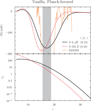
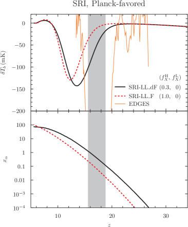
Figure 10: 21 cm backgrounds (top) and the Ly$\alpha$ coupling coefficients (bottom) of models that fit PLD best (those marked by arrows in Fig 7), selected from the vanilla and SRI. The shade indicates the redshift bin of the 500-mK absorption trough claimed by the EDGES observation. The EDGES data is shown in orange, thin solid line.

Compared to the signal interpreted by the EDGES team, none of the the global $\delta T_{b}$’s of our models can match the EDGES’ one in the amplitude and the spectral shape. Among the tested models, V-L_dF provides $\delta T_{b}$ closest to the EDGES data. However, this is as closest as one can get to the amplitude of the EDGES absorption trough in the $\Lambda$CDM, because the case is tuned to produce the coldest $T_{{\rm K}}$ and the largest $x_{\alpha}$, with $x_{\alpha}\simeq 5-20$ in the EDGES window, with a reionization history well under the PLD constraint. The SRI models are terrible in matching the EDGES data, mainly due to the shift of the absorption dip caused by the nature of the Pop III SED of LMACH stars dominating this era. The SRII models are as bad as SRI models in matching the EDGES data within the trough window, mainly due to the dominance of MH stars with Pop III SED. Note that all the cases are tuned to produce maximum possible $\left|\delta T_{b}\right|$ in absorption with $f_{X}^{{\rm L}}=0$ (SRI) and $f_{X}^{{\rm L}}=f_{X}^{{\rm M}}=0$ (SRII) with non-zero $f_{X}^{{\rm H}}$. Any addition of non-zero X-ray heating will increase $T_{{\rm K}}$ from these null-heating cases to reduce $\left|\delta T_{b}\right|$ and worsen the mismatch between the EDGES’ interpretation and the theory.

The SRII models produce $\delta T_{b}$ that is the most peculiar in the spectral shape, because across the full EDGES window ($14\lesssim z\lesssim 24$) $\delta T_{b}(z)$ is almost featureless without much variation. It would be even possible that the process of foreground-removal, utilizing the spectral smoothness of the foreground, from the observed signal could completely remove the true EoR (or Dark Ages) signal at $z\gtrsim 14$ or $\nu\lesssim 95\,{\rm MHz}$ to yield only a null result. The limited amplitude of the absorption depth, $\left|\delta T_{b}(z\gtrsim 14)\right|\lesssim 60\,{\rm mK}$, and the featureless spectral shape place our SRII model category as the one that disagrees with the EDGES data most. Considering the excellent agreement of many two-phase reionization models in the SRII category with the PLD polarization data, rather extreme alternative explanations to the standard model are required to explain the EDGES data in order to accept SRII. If SRII were the right model, the excess radio background or other alternatives should (1) almost solely contribute to the absorption trough of $\sim 500\,{\rm mK}$ because even the small ($\lesssim 60\,{\rm mK}$) absorption signal is likely to be removed in the foreground removal process and (2) offset the possible absorption depth of $\delta T_{b}\sim-100\,{\rm mK}$ at $z\sim 12$ in case X-ray heating is inefficient. Obviously, independent observations such as the 21 cm intensity mapping by radio interferometers will help to settle this issue.

We note that the limited amplitude and the featureless spectral shape of the global $\delta T_{b}(z)$ in SRII models are a novel result, and such features are in large disagreement with other studies that also implement the LW feedback on Pop III stars inside MHs to investigate its impact on $\delta T_{b}$ (Mirocha et al. 2018; Mirocha & Furlanetto 2019; Mebane et al. 2020; Qin et al. 2020a, 2021). Let us explain the major reason for such a discrepancy. A big difference lies among this work and others in the LW feedback is implemented. As described in Section 2.2.3, we assume that there exists a threshold value of $J_{{\rm LW}}$ such that star formation inside MHs are fully suppressed as long as $J_{{\rm LW}}>J_{{\rm LW,\,th}}$, based on the observed abrupt change in $M_{{\rm min}}$ (the minimum mass of star-forming halos) and $T_{{\rm vir,\,min}}$ (the minimum virial temperature of star-forming halos) of star-forming MHs as $J_{{\rm LW}}$ varies across the value $J_{{\rm LW}}\sim 0.1\times 10^{-21}\,{\rm erg\,s^{-1}\,cm^{-2}\,Hz^{-1}\,sr^{-1}}$ in Yoshida et al. (2003) and O’Shea & Norman (2008). In contrast, other studies usually adopt a prescription where $M_{{\rm min}}$ and consequently $T_{{\rm vir,\,min}}$ are smooth functions of $J_{{\rm LW}}$. While numerical coefficients vary somewhat in the literature (e.g. see difference between Fialkov et al. 2013 and Schauer et al. 2020), the commonly used functional form for $M_{{\rm min}}$ is either a redshift-independent one (advocated by Machacek et al. 2001 and Wise & Abel 2007),

$$M_{{\rm min}}/M_{\odot}=2.5\times 10^{5}\left[1+6.8\left(4\pi J_{21}\right)^{0.47}\right]$$ (33)

where $J_{21}\equiv J_{{\rm LW}}/(10^{-21}\,{\rm erg\,s^{-1}\,cm^{-2}\,Hz^{-1}\,sr^{-1}})$, or a redshift-dependent one (Fialkov et al. 2013; Qin et al. 2021; Visbal et al. 2020),

$$M_{{\rm min}}/M_{\odot}$$

$$=2.5\times 10^{5}\left(\frac{1+z}{26}\right)^{-1.5}f(v_{{\rm bc}};\,z)\left[1+6.96J_{21}^{0.47}\right]$$ (34)

where $f(v_{{\rm bc}};\,z)\geq 1$ is an additional factor accounting for the suppression of star formation due to the baryon-dark matter streaming velocity (Tseliakhovich & Hirata 2010; Ahn 2016). If one uses one of equations (33) and (34), the effective $J_{{\rm LW,\,th}}$ is much larger than $J_{{\rm 21}}=0.1$ and thus star formation inside MHs will become much stronger than our prescription at a given $J_{{\rm LW}}$. Therefore, studies adopting equation (34), e.g. Fialkov et al. (2013), Qin et al. (2021) and Visbal et al. (2020), find Ly$\alpha$ intensity much stronger than our prediction, $x_{\alpha}(z\gtrsim 14)\lesssim 0.5$, in SRII models. Consequently, these studies find that MH stars bring the absorption dip occur much earlier at $z\sim 16-18$ than in cases without MH stars (Mebane et al. 2020; Qin et al. 2020a) and with amplitude easily reaching $\left|\delta T_{b}\right|\gtrsim 100\,{\rm mK}$. However, we stress that if one focuses on $T_{{\rm vir,\,min}}$, O’Shea & Norman (2008) clearly shows $T_{{\rm vir,\,min}}\simeq 8000\,{\rm K}$ when $J_{21}\simeq 0.1$. If we take this result and extrapolate to any other redshift, one can instead conclude that $J_{{\rm LW,\,th}}$ should lie around $J_{21}=0.1$. In this paper, we parameterize $J_{{\rm LW,\,th}}$ but to a limited value of $J_{{\rm LW,\,th,\,21}}\leq 0.1$, respecting the results of Yoshida et al. (2003) and O’Shea & Norman (2008). Of course, one cannot exclude one LW feedback scheme against another at the moment, because there is practically no observational constraint on ultra high-$z$ ($z\gtrsim 14)$ radiation sources.

The success of our SRII models in producing two-stage reionization models, which are somewhat favored by PLD against vanilla and SRI models, can be taken as a hint that SRII models may represent the reality including how the LW feedback operates in nature. If this were true, the gross disagreement of the global $\delta T_{b}(z)$ of SRII models with the EDGES result would be hardly conceivable in the standard model or the EDGES result could be an incorrect claim. Further study is warranted.

4 Summary and Conclusion

We studied three types of reionization models semi-analytically: the vanilla, SRI and SRII models. SRI and SRII models implement the negative feedback effects on star formation inside LMACHS (SRI, SRII) and MHs (SRII only), namely the Jeans-mass filtering due to photoionization (LMACH, MH) and the LW feedback (MH). As long as LMACHs and MHs host Pop III stars and dominate the era of $z\gtrsim 14$, we find that $\delta T_{b}$ is constrained to $-50\,{\rm mK}\lesssim\delta T_{b}<0$ in both SRI and SRII models that is in stark contrast with the $\sim 500\,{\rm mK}$ absorption trough claimed by the EDGES. $\delta T_{b}$’s predicted by SRII models are almost featureless in its spectral shape for $z\gtrsim 14$ ($\nu\lesssim 95\,{\rm MHz}$) due to the strong self-regulation of star formation inside MHs by the LW background built up my MHs.

At this stage with the PLD being the most accurate large-scale-CMB anisotropy observation, we find that all three models can provide acceptable reionization scenarios. Especially, we find that SRII models with substantial high-redshift ($z\gtrsim 15$) ionization tails are as favored as those models without such tails, if corresponding $C_{l}^{{\rm EE}}$ is analyzed against the $C_{l}^{{\rm EE}}$ of the PLD. SRII models have the two-stage ionization feature, the high-redshift slow-ionization stage and the low-redshift fast-ionization stage, which seems more favored by PLD than tail-less reionization models even though this tendency is largely uncertain in PLD. In conclusion, SRII models with substantial high-$z$ ionization tails should NOT be ruled out as claimed by Planck Collaboration et al. (2018). Our $C_{l}^{{\rm EE}}$-only analysis favors models with $\tau_{{\rm es}}\simeq 0.055-0.064$, which is relatively larger than the $C_{l}^{{\rm EE}}$-only inference by Planck Collaboration et al. (2018), $\tau_{{\rm es}}=0.0504_{-0.0079}^{+0.0050}$. This issue needs to be investigated further.

In light of the peculiarity of $\delta T_{b}$ but the good agreement with PLD-$C_{l}^{{\rm EE}}$ and the hint of two-stage reionization, we stress that SRII models should be considered more seriously. Such a disagreement with the EDGES data requires a change in the standard $\Lambda$CDM model or the “interpretation” of the EDGES data. Even though many statistical analyses have been already carried out by accepting the full result (e.g. Mebane et al. 2020) or a part of the result (Qin et al. 2020a: only the redshift window of the absorption trough is taken as the possible location for the absorption dip) of EDGES, we question the foreground-removal scheme of the EDGES team as Hills et al. (2018) and Tauscher et al. 2020 did. The claimed signal is indeed a result of extracting an arbitrary smooth signal from the residual signal (Fig 1b in Bowman et al. 2018) after the foreground removal. There is no guarantee that a combination of log-power-law spectral curves could completely remove the foreground, and such an additional arbitrary removal seems even more dubious. It would be even harder to probe the EoR signal if nature were indeed described by our SRII models, because the featureless spectral shape at $z\gtrsim 14$ of the models is going to be removed by any foreground-removal scheme utilizing the spectral smoothness. In this regard, probing the dipole anisotropy of $\delta T_{b}$ seems very promising (Deshpande 2018; Trombetti et al. 2020), because the dipole moment is caused by the monopole moment seen by an observer with a peculiar motion and thus can be an independent probe of the global $\delta T_{b}$.

It is therefore crucial to carry out higher-precision CMB observation and the 21-cm intensity mapping to further constrain the reionization history. A superb CMB polarization apparatus limited only by the cosmic variance (for all $2\leq l\lesssim 200$), LiteBIRD (Lite (Light) satellite for the studies of B-mode polarization and Inflation from cosmic background Radiation Detection), is under way, which will significantly sharpen the constraint on the reionization history. Many different reionization histories can share the same $\tau_{{\rm es}}$ and $z_{{\rm ov}}$ (see e.g. Fig. 4b in Ahn et al. 2012), and breaking this degeneracy seems elusive with the PLD at this low-$\tau_{{\rm es}}$ era but will become more feasible with such a high-precision CMB observation. The boost of $C_{8\lesssim l\lesssim 24}^{{\rm EE}}$ of SRII models relative to that of the vanilla and SRII models is of particular interest. The 21-cm intensity mapping will be able to probe large-scale fluctuation of HI density when large H II regions are produced during EoR. The high-redshift regime with $z\gtrsim 15$ is more in the Dark Ages without too much ionization in typical reionization scenarios, while some SRII models produce a substantial amount of ionization. Nevertheless, SRII models predict only small-size H II regions by MHs (Ahn et al. 2012) that might not be imaged individually by radio interferometers. If future CMB observations favored two-stage reionization but radio interferometry did not reveal any noticeable H II bubbles at high redshift, SRII models would be the strongest candidate to explain both. We will investigate detailed observational prospects in the future.

References

- Abel et al. (2000) Abel, T., Bryan, G. L., & Norman, M. L. 2000, ApJ, 540, 39, doi: 10.1086/309295
- Ahn (2016) Ahn, K. 2016, ApJ, 830, 68, doi: 10.3847/0004-637X/830/2/68
- Ahn et al. (2012) Ahn, K., Iliev, I. T., Shapiro, P. R., et al. 2012, ApJ, 756, L16, doi: 10.1088/2041-8205/756/1/L16
- Ahn et al. (2015) Ahn, K., Iliev, I. T., Shapiro, P. R., & Srisawat, C. 2015, MNRAS, 450, 1486, doi: 10.1093/mnras/stv704
- Ahn et al. (2009) Ahn, K., Shapiro, P. R., Iliev, I. T., Mellema, G., & Pen, U. 2009, ApJ, 695, 1430, doi: 10.1088/0004-637X/695/2/1430
- Ahn et al. (2014) Ahn, K., Xu, H., Norman, M. L., Alvarez, M. A., & Wise, J. H. 2014, ArXiv e-prints. https://arxiv.org/abs/1405.2085
- Barkana (2018) Barkana, R. 2018, Nature, 555, 71, doi: 10.1038/nature25791
- Barkana & Loeb (2001) Barkana, R., & Loeb, A. 2001, Phys. Rep., 349, 125
- Battaglia et al. (2013) Battaglia, N., Natarajan, A., Trac, H., Cen, R., & Loeb, A. 2013, ApJ, 776, 83, doi: 10.1088/0004-637X/776/2/83
- Becker et al. (2001) Becker, R. H., Fan, X., White, R. L., et al. 2001, AJ, 122, 2850, doi: 10.1086/324231
- Bernardi et al. (2015) Bernardi, G., McQuinn, M., & Greenhill, L. J. 2015, ApJ, 799, 90, doi: 10.1088/0004-637X/799/1/90
- Bolton & Haehnelt (2007) Bolton, J. S., & Haehnelt, M. G. 2007, MNRAS, 382, 325, doi: 10.1111/j.1365-2966.2007.12372.x
- Bowman & Rogers (2010) Bowman, J. D., & Rogers, A. E. E. 2010, Nature, 468, 796, doi: 10.1038/nature09601
- Bowman et al. (2018) Bowman, J. D., Rogers, A. E. E., Monsalve, R. A., Mozdzen, T. J., & Mahesh, N. 2018, Nature, 555, 67, doi: 10.1038/nature25792
- Bromm et al. (2002) Bromm, V., Coppi, P. S., & Larson, R. B. 2002, ApJ, 564, 23, doi: 10.1086/323947
- Calverley et al. (2011) Calverley, A. P., Becker, G. D., Haehnelt, M. G., & Bolton, J. S. 2011, MNRAS, 412, 2543, doi: 10.1111/j.1365-2966.2010.18072.x
- Cen (2003) Cen, R. 2003, ApJ, 591, 12, doi: 10.1086/375217
- Chen & Miralda-Escudé (2004) Chen, X., & Miralda-Escudé, J. 2004, ApJ, 602, 1, doi: 10.1086/380829
- Chuzhoy & Shapiro (2006) Chuzhoy, L., & Shapiro, P. R. 2006, ApJ, 651, 1, doi: 10.1086/507670
- Chuzhoy & Shapiro (2007) Chuzhoy, L., & Shapiro, P. R. 2007, ApJ, 655, 843, doi: 10.1086/510146
- Ciardi & Salvaterra (2007) Ciardi, B., & Salvaterra, R. 2007, MNRAS, 381, 1137, doi: 10.1111/j.1365-2966.2007.12303.x
- Deshpande (2018) Deshpande, A. A. 2018, ApJ, 866, L7, doi: 10.3847/2041-8213/aae318
- Dijkstra et al. (2004) Dijkstra, M., Haiman, Z., Rees, M. J., & Weinberg, D. H. 2004, ApJ, 601, 666, doi: 10.1086/380603
- Dodelson (2003) Dodelson, S. 2003, Modern cosmology (Modern cosmology / Scott Dodelson. Amsterdam (Netherlands): Academic Press. ISBN 0-12-219141-2, 2003, XIII + 440 p.)
- Efstathiou (1992) Efstathiou, G. 1992, MNRAS, 256, 43P
- Ewall-Wice et al. (2018) Ewall-Wice, A., Chang, T. C., Lazio, J., et al. 2018, ApJ, 868, 63, doi: 10.3847/1538-4357/aae51d
- Fan et al. (2002) Fan, X., Narayanan, V. K., Strauss, M. A., et al. 2002, AJ, 123, 1247, doi: 10.1086/339030
- Feng & Holder (2018) Feng, C., & Holder, G. 2018, ApJ, 858, L17, doi: 10.3847/2041-8213/aac0fe
- Fialkov et al. (2013) Fialkov, A., Barkana, R., Visbal, E., Tseliakhovich, D., & Hirata, C. M. 2013, MNRAS, 432, 2909, doi: 10.1093/mnras/stt650
- Field (1958) Field, G. B. 1958, Proceedings of the IRE, 46, 240, doi: 10.1109/JRPROC.1958.286741
- Furlanetto (2006) Furlanetto, S. R. 2006, MNRAS, 371, 867, doi: 10.1111/j.1365-2966.2006.10725.x
- Ghara & Mellema (2020) Ghara, R., & Mellema, G. 2020, MNRAS, 492, 634, doi: 10.1093/mnras/stz3513
- Ghara et al. (2020) Ghara, R., Giri, S. K., Mellema, G., et al. 2020, MNRAS, 493, 4728, doi: 10.1093/mnras/staa487
- Glover (2013) Glover, S. 2013, The First Stars, ed. T. Wiklind, B. Mobasher, & V. Bromm, Vol. 396, 103. https://ui.adsabs.harvard.edu/abs/2013ASSL..396..103G
- Gnedin (2000) Gnedin, N. Y. 2000, ApJ, 542, 535, doi: 10.1086/317042
- Gnedin & Hui (1998) Gnedin, N. Y., & Hui, L. 1998, MNRAS, 296, 44
- Greif et al. (2007) Greif, T. H., Johnson, J. L., Bromm, V., & Klessen, R. S. 2007, ApJ, 670, 1, doi: 10.1086/522028
- Grimm et al. (2003) Grimm, H. J., Gilfanov, M., & Sunyaev, R. 2003, MNRAS, 339, 793, doi: 10.1046/j.1365-8711.2003.06224.x
- Haardt & Madau (1996) Haardt, F., & Madau, P. 1996, ApJ, 461, 20, doi: 10.1086/177035
- Haiman & Holder (2003) Haiman, Z., & Holder, G. P. 2003, ApJ, 595, 1
- Haiman & Knox (1999) Haiman, Z., & Knox, L. 1999, in ASP Conf. Ser. 181: Microwave Foregrounds, ed. A. de Oliveira-Costa & M. Tegmark, 227–+
- Haiman & Loeb (1997) Haiman, Z., & Loeb, A. 1997, ApJ, 483, 21, doi: 10.1086/304238
- Haiman et al. (1997) Haiman, Z., Rees, M. J., & Loeb, A. 1997, ApJ, 476, 458, doi: 10.1086/303647
- Heinrich & Hu (2018) Heinrich, C., & Hu, W. 2018, Phys. Rev. D, 98, 063514, doi: 10.1103/PhysRevD.98.063514
- Hill & Baxter (2018) Hill, J. C., & Baxter, E. J. 2018, J. Cosmology Astropart. Phys, 2018, 037, doi: 10.1088/1475-7516/2018/08/037
- Hills et al. (2018) Hills, R., Kulkarni, G., Meerburg, P. D., & Puchwein, E. 2018, Nature, 564, E32, doi: 10.1038/s41586-018-0796-5
- Hinshaw et al. (2013) Hinshaw, G., Larson, D., Komatsu, E., et al. 2013, ApJS, 208, 19, doi: 10.1088/0067-0049/208/2/19
- Hirano et al. (2015) Hirano, S., Hosokawa, T., Yoshida, N., Omukai, K., & Yorke, H. W. 2015, MNRAS, 448, 568, doi: 10.1093/mnras/stv044
- Hirano et al. (2014) Hirano, S., Hosokawa, T., Yoshida, N., et al. 2014, ApJ, 781, 60, doi: 10.1088/0004-637X/781/2/60
- Hirata (2006) Hirata, C. M. 2006, MNRAS, 367, 259, doi: 10.1111/j.1365-2966.2005.09949.x
- Hu & White (1997) Hu, W., & White, M. 1997, Phys. Rev. D, 56, 596
- Iliev et al. (2007) Iliev, I. T., Mellema, G., Shapiro, P. R., & Pen, U. 2007, MNRAS, 376, 534, doi: 10.1111/j.1365-2966.2007.11482.x
- Iliev et al. (2005) Iliev, I. T., Scannapieco, E., & Shapiro, P. R. 2005, ApJ, 624, 491
- Kimm et al. (2017) Kimm, T., Katz, H., Haehnelt, M., et al. 2017, MNRAS, 466, 4826, doi: 10.1093/mnras/stx052
- Kohler et al. (2007) Kohler, K., Gnedin, N. Y., & Hamilton, A. J. S. 2007, ApJ, 657, 15, doi: 10.1086/509907
- Lewis et al. (2000) Lewis, A., Challinor, A., & Lasenby, A. 2000, Astrophys. J., 538, 473, doi: 10.1086/309179
- Loeb & Barkana (2001) Loeb, A., & Barkana, R. 2001, ARA&A, 39, 19, doi: 10.1146/annurev.astro.39.1.19
- Machacek et al. (2001) Machacek, M. E., Bryan, G. L., & Abel, T. 2001, ApJ, 548, 509, doi: 10.1086/319014
- Mao et al. (2020) Mao, Y., Koda, J., Shapiro, P. R., et al. 2020, MNRAS, 491, 1600, doi: 10.1093/mnras/stz2986
- Mebane et al. (2020) Mebane, R. H., Mirocha, J., & Furlanetto, S. R. 2020, MNRAS, 493, 1217, doi: 10.1093/mnras/staa280
- Mertens et al. (2020) Mertens, F. G., Mevius, M., Koopmans, L. V. E., et al. 2020, MNRAS, 493, 1662, doi: 10.1093/mnras/staa327
- Mesinger et al. (2011) Mesinger, A., Furlanetto, S., & Cen, R. 2011, MNRAS, 411, 955, doi: 10.1111/j.1365-2966.2010.17731.x
- Mesinger et al. (2012) Mesinger, A., McQuinn, M., & Spergel, D. N. 2012, MNRAS, 422, 1403, doi: 10.1111/j.1365-2966.2012.20713.x
- Millea & Bouchet (2018) Millea, M., & Bouchet, F. 2018, A&A, 617, A96, doi: 10.1051/0004-6361/201833288
- Miranda et al. (2017) Miranda, V., Lidz, A., Heinrich, C. H., & Hu, W. 2017, MNRAS, 467, 4050, doi: 10.1093/mnras/stx306
- Mirocha (2014) Mirocha, J. 2014, MNRAS, 443, 1211, doi: 10.1093/mnras/stu1193
- Mirocha & Furlanetto (2019) Mirocha, J., & Furlanetto, S. R. 2019, MNRAS, 483, 1980, doi: 10.1093/mnras/sty3260
- Mirocha et al. (2018) Mirocha, J., Mebane, R. H., Furlanetto, S. R., Singal, K., & Trinh, D. 2018, MNRAS, 478, 5591, doi: 10.1093/mnras/sty1388
- Mittal & Kulkarni (2020) Mittal, S., & Kulkarni, G. 2020, MNRAS, doi: 10.1093/mnras/staa3811
- Monsalve et al. (2017) Monsalve, R. A., Rogers, A. E. E., Bowman, J. D., & Mozdzen, T. J. 2017, ApJ, 847, 64, doi: 10.3847/1538-4357/aa88d1
- Mortonson & Hu (2008) Mortonson, M. J., & Hu, W. 2008, Astrophys. J., 672, 737, doi: 10.1086/523958
- Nasirudin et al. (2020) Nasirudin, A., Iliev, I. T., & Ahn, K. 2020, MNRAS, 494, 3294, doi: 10.1093/mnras/staa853
- Navarro & Steinmetz (1997) Navarro, J. F., & Steinmetz, M. 1997, ApJ, 478, 13, doi: 10.1086/303763
- O’Shea & Norman (2008) O’Shea, B. W., & Norman, M. L. 2008, ApJ, 673, 14, doi: 10.1086/524006
- Park et al. (2013) Park, H., Shapiro, P. R., Komatsu, E., et al. 2013, ApJ, 769, 93, doi: 10.1088/0004-637X/769/2/93
- Pawlik et al. (2009) Pawlik, A. H., Schaye, J., & van Scherpenzeel, E. 2009, MNRAS, 394, 1812, doi: 10.1111/j.1365-2966.2009.14486.x
- Pentericci et al. (2011) Pentericci, L., Fontana, A., Vanzella, E., et al. 2011, ApJ, 743, 132, doi: 10.1088/0004-637X/743/2/132
- Planck Collaboration et al. (2013) Planck Collaboration, Ade, P. A. R., Aghanim, N., et al. 2013, ArXiv e-prints. https://arxiv.org/abs/1303.5076
- Planck Collaboration et al. (2016) Planck Collaboration, Ade, P. A. R., Aghanim, N., et al. 2016, A&A, 594, A13, doi: 10.1051/0004-6361/201525830
- Planck Collaboration et al. (2018) Planck Collaboration, Aghanim, N., Akrami, Y., et al. 2018, arXiv e-prints. https://arxiv.org/abs/1807.06209
- Pritchard & Furlanetto (2006) Pritchard, J. R., & Furlanetto, S. R. 2006, MNRAS, 367, 1057, doi: 10.1111/j.1365-2966.2006.10028.x
- Qin et al. (2021) Qin, Y., Mesinger, A., Greig, B., & Park, J. 2021, MNRAS, 501, 4748, doi: 10.1093/mnras/staa3408
- Qin et al. (2020a) Qin, Y., Mesinger, A., Park, J., Greig, B., & Muñoz, J. B. 2020a, MNRAS, 495, 123, doi: 10.1093/mnras/staa1131
- Qin et al. (2020b) Qin, Y., Poulin, V., Mesinger, A., et al. 2020b, MNRAS, 499, 550, doi: 10.1093/mnras/staa2797
- Reichardt et al. (2012) Reichardt, C. L., Shaw, L., Zahn, O., et al. 2012, ApJ, 755, 70, doi: 10.1088/0004-637X/755/1/70
- Schauer et al. (2020) Schauer, A. T. P., Glover, S. C. O., Klessen, R. S., & Clark, P. 2020, arXiv e-prints, arXiv:2008.05663. https://arxiv.org/abs/2008.05663
- Shapiro et al. (1994) Shapiro, P. R., Giroux, M. L., & Babul, A. 1994, ApJ, 427, 25, doi: 10.1086/174120
- Sheth & Tormen (1999) Sheth, R. K., & Tormen, G. 1999, MNRAS, 308, 119, doi: 10.1046/j.1365-8711.1999.02692.x
- Singh et al. (2018) Singh, S., Subrahmanyan, R., Udaya Shankar, N., et al. 2018, ApJ, 858, 54, doi: 10.3847/1538-4357/aabae1
- So et al. (2014) So, G. C., Norman, M. L., Reynolds, D. R., & Wise, J. H. 2014, ApJ, 789, 149, doi: 10.1088/0004-637X/789/2/149
- Stacy et al. (2010) Stacy, A., Greif, T. H., & Bromm, V. 2010, MNRAS, 403, 45, doi: 10.1111/j.1365-2966.2009.16113.x
- Tashiro et al. (2014) Tashiro, H., Kadota, K., & Silk, J. 2014, Phys. Rev. D, 90, 083522, doi: 10.1103/PhysRevD.90.083522
- Tauscher et al. (2020) Tauscher, K., Rapetti, D., & Burns, J. O. 2020, ApJ, 897, 132, doi: 10.3847/1538-4357/ab9a3f
- Thoul & Weinberg (1996) Thoul, A. A., & Weinberg, D. H. 1996, ApJ, 465, 608, doi: 10.1086/177446
- Trac & Cen (2007) Trac, H., & Cen, R. 2007, ApJ, 671, 1, doi: 10.1086/522566
- Trombetti et al. (2020) Trombetti, T., Burigana, C., & Chierici, F. 2020, arXiv e-prints, arXiv:2007.02292. https://arxiv.org/abs/2007.02292
- Tseliakhovich et al. (2011) Tseliakhovich, D., Barkana, R., & Hirata, C. M. 2011, MNRAS, 418, 906, doi: 10.1111/j.1365-2966.2011.19541.x
- Tseliakhovich & Hirata (2010) Tseliakhovich, D., & Hirata, C. 2010, Phys. Rev. D, 82, 083520, doi: 10.1103/PhysRevD.82.083520
- Turk et al. (2009) Turk, M. J., Abel, T., & O’Shea, B. 2009, Science, 325, 601, doi: 10.1126/science.1173540
- Visbal et al. (2020) Visbal, E., Bryan, G. L., & Haiman, Z. 2020, ApJ, 897, 95, doi: 10.3847/1538-4357/ab994e
- Whalen et al. (2008) Whalen, D., van Veelen, B., O’Shea, B. W., & Norman, M. L. 2008, ApJ, 682, 49, doi: 10.1086/589643
- Wise & Abel (2007) Wise, J. H., & Abel, T. 2007, ApJ, 671, 1559, doi: 10.1086/522876
- Wouthuysen (1952) Wouthuysen, S. A. 1952, AJ, 57, 31, doi: 10.1086/106661
- Yoshida et al. (2003) Yoshida, N., Abel, T., Hernquist, L., & Sugiyama, N. 2003, Astrophys. J., 592, 645, doi: 10.1086/375810
- Yoshida et al. (2007) Yoshida, N., Oh, S. P., Kitayama, T., & Hernquist, L. 2007, ApJ, 663, 687, doi: 10.1086/518227
- Zahn et al. (2012) Zahn, O., Reichardt, C. L., Shaw, L., et al. 2012, ApJ, 756, 65, doi: 10.1088/0004-637X/756/1/65
- Zygelman (2005) Zygelman, B. 2005, ApJ, 622, 1356, doi: 10.1086/427682