The Herschel Orion Protostar Survey: Far-Infrared Photometry and Colors
of Protostars and Their Variations across Orion A and B

Abstract

The degree to which the properties of protostars are affected by environment remains an open question. To investigate this, we look at the Orion A and B molecular clouds, home to most of the protostars within 500 pc. At $\sim$ 400 pc, Orion is close enough to distinguish individual protostars across a range of environments in terms of both the stellar and gas projected densities. As part of the Herschel Orion Protostar Survey (HOPS), we used the Photodetector Array Camera and Spectrometer (PACS) to map 108 partially overlapping square fields with edge lengths of 5$\arcmin$ or 8$\arcmin$ and measure the 70 µm and 160 µm flux densities of 338 protostars within them. In this paper we examine how these flux densities and their ratio depend on evolutionary state and environment within the Orion complex. We show that Class 0 protostars occupy a region of the 70 µm flux density versus 160 µm to 70 µm flux density ratio diagram that is distinct from their more evolved counterparts. We then present evidence that the Integral-Shaped Filament (ISF) and Orion B contain protostars with more massive envelopes than those in the more sparsely populated LDN 1641 region. This can be interpreted as evidence for increasing star formation rates in the ISF and Orion B or as a tendency for more massive envelopes to be inherited from denser birth environments. We also provide technical details about the map-making and photometric procedures used in the HOPS program.

1 Introduction

A complete picture of star formation, from the gravitational collapse of a molecular cloud to the dispersal of the circumstellar envelope and disk, is a fundamental part of our understanding of our cosmic origins. In recent years, space-based mid- to far-infrared (far-IR) surveys have mapped a large sample of protostars in nearby molecular clouds, enabling detailed studies of protostellar evolution (Dunham et al., 2014). In this protostellar phase, a dusty infalling envelope and a nascent protoplanetary disk surround an accreting protostar. The envelope absorbs short-wavelength radiation from the central protostar and reprocesses most of the luminosity to far-IR wavelengths (e.g., Whitney et al., 2003). The protostar drives a bipolar outflow that may evacuate cavities in the envelope, allowing some of the shorter wavelength radiation to escape. After $\sim$ 0.5 Myr, the envelope disappears and the protostellar phase is over. It is not clear to what extent the dissipation of the envelopes is driven by feedback from outflows or the depletion of the reservoir of gas in the environment.

Far-IR observations are an essential tool for understanding the protostellar phase. Protostars typically radiate most of their luminosity in the far IR, the dusty star-forming environment also emits strongly at far-IR wavelengths, and far-IR photons easily penetrate this dust to reach the observer. During the protostellar stage, the forming star is still strongly connected to the local environment, and variations in the gas environment may alter the trajectory of protostellar evolution. A detailed characterization of protostellar evolution in the far IR thus allows us to better understand the role of environment in star formation.

This link between protostars and their surroundings presents challenges to observational studies. Observers must disentangle environmental emission from that of the protostar. The spatial scales of the central object, disk, envelope, and outflows range from less than one AU to thousands of AU. Observational strategies must account for morphologies that are complex at both compact and extended scales.

The Herschel Orion Protostar Survey (HOPS; PI: S. T. Megeath) was a 200 hour open-time key program of the Herschel Space Observatory (Pilbratt et al., 2010). HOPS used the Photodetector Array Camera and Spectrometer (PACS) instrument (Poglitsch et al., 2010) to obtain 70 and 160 µm images (with angular resolutions of 5.2″ and 12″, respectively) and 55–200 µm spectra of protostars identified in the Spitzer Space Telescope survey of Orion (Megeath et al., 2012, 2016).

The use of Herschel data facilitates the direct measurement of emission from the protostellar envelopes, sampling the peaks of their spectral energy distributions (SEDs). The unprecedented sensitivity afforded by Herschel at far-IR wavelengths allowed us to efficiently survey a large number of protostars (Furlan et al., 2016) and discover new ones (Stutz et al., 2013). We supplemented these data with imaging, photometry, and spectroscopy from 1.2 to 870 µm. Multiwavelength data allow us to constrain the protostars and the properties of their envelopes (Furlan et al., 2016).

A major benefit to the study of Orion is that it contains a large sample of protostars in a single cloud complex. Furlan et al. (2016) tabulated 319 protostars (in a sample of 330 young stellar objects or YSOs) in Orion alone, while Dunham et al. (2013) used Spitzer data to find 230 protostars in 18 other nearby ($<$ 500 pc) molecular clouds.

A second benefit to the study of Orion is that, at approximately 400 pc, it is relatively nearby. According to Kounkel et al. (2018), our targets mostly lie at distances from 389 pc to 417 pc, except for a few at 345 pc; see further discussion below. Herschel data therefore provide sufficiently high spatial resolution to isolate individual protostellar envelopes in a single comparatively high-mass ($\sim$ 10⁵ $M_{\sun}$; e.g., Stutz & Kainulainen 2015) and nearby cloud, even in clustered regions. The only similarly nearby and massive cloud is the California molecular cloud (Lada et al., 2009), but it contains far fewer YSOs. At the distance of Orion, the angular resolution of PACS corresponds to distances of 2100 and 4800 AU for the 70 and 160 µm channels, respectively.

A third benefit to the study of Orion is that it contains significantly different environments, from isolated cold globules to rich clusters. There are two common observational measures of environment. First, there are the environmental conditions set by the properties of the natal molecular gas, particularly the dense gas. Second, there are environmental variations traced by the protostars, including the densities of young stars and the systematic changes in their properties. These protostars and their properties have been quantified with Spitzer data (Megeath et al., 2012, 2016) and Herschel data from HOPS (Furlan et al., 2016).

With Herschel observations at longer wavelengths and of wider fields than included in HOPS, Stutz & Kainulainen (2015) measured the column density ($N_{\rm H}$) and mass distributions across Orion A, quantifying environmental differences. They found that the column density probability distribution functions vary with location. Furthermore, Stutz & Gould (2016) and Stutz (2018) found that the mass per unit length ($M/L$) varies significantly across Orion A, with the Orion Nebula Cluster (ONC) having a higher $M/L$ than the Integral Shaped Filament (ISF), and the ISF having a higher $M/L$ than LDN 1641. These column density and mass variations imply variations in the volume density and gravitational potential across the cloud.

Environmental variations are also found in the radial velocities of the gas. González Lobos & Stutz (2019) showed that gas radial velocities in both high- and low-density tracers show significant variations within the ISF. In particular, the northern portion has more centrally concentrated gas with stronger overall velocity gradients compared to the southern portion, which transitions to the LDN 1641 region. Systematic variations of the temperatures, line widths, and densities of cores across Orion A were also found by Wilson et al. (1999).

Turning to the stellar content, the observed properties of the protostars vary with environment. Kryukova et al. (2012) found variations in the Orion clouds, where protostars are more luminous in dense regions. Stutz & Kainulainen (2015) found that the fraction of protostars in the young Class 0 phase varies systematically with changes in environment as indicated by variations in the slope of the dust column density probability distribution function ($N$-PDF) across the region. The variation in this fraction may result from differences in the star formation history between these regions, as also suggested by Fischer et al. (2017), the influence of feedback (Sadavoy et al., 2014), or variations in infall rates of the protostars due to variations in the densities of their birth environments (Kryukova et al., 2012, 2014; Dunham et al., 2014).

This paper is part of a series describing results from HOPS. These papers include evolutionary studies of protostars via modeling of their SEDs (Furlan et al., 2016; Fischer et al., 2017), the analysis of far-IR protostellar spectra (Manoj et al., 2013, 2016), the discovery and characterization of the youngest protostars (Stutz et al., 2013; Tobin et al., 2015, 2016; Karnath et al., 2020), a study of multiplicity in the Orion YSOs (Kounkel et al., 2016), progress on understanding outburst phenomena in protostars (Fischer et al., 2012; Safron et al., 2015; Fischer et al., 2019), and detailed studies of the active OMC 2/3 region (Furlan et al., 2014; González-García et al., 2016; Osorio et al., 2017).

Here we present the 70 and 160 µm photometry obtained with Herschel and first reported by Furlan et al. (2016) as part of their effort to model the SEDs of the Orion protostars with Herschel and other multiwavelength data. Section 2 reviews the main aspects of the sample selection and observing strategy, pointing the reader to the Appendix for the HOPS catalog and previously unpublished descriptions of the map-making and photometric techniques that lie at the foundation of Furlan et al. (2016) and other HOPS papers.

Section 3 uses the HOPS 70 and 160 µm photometry to analyze protostellar properties across the Orion complex, including their dependence on evolutionary stage and location within Orion. In part, it relies on the SED classification by Furlan et al. (2016). Section 4 contains our discussion, and our conclusions are summarized in Section 5. Our maps, photometry, SEDs, and model fits to the SEDs can be found at the Infrared Science Archive (IRSA).

2 Sample Selection

The HOPS sources are numbered from 0 to 409. Most were identified as protostars in the Spitzer survey of Orion. The Spitzer protostar sample was defined and described by Megeath et al. (2012), with minor modification by Megeath et al. (2016). Kryukova et al. (2012) discussed the development of the initial criteria. Their identification relied on Spitzer 3.6–24 µm photometry merged with 1–2 µm photometry from the Two Micron All Sky Survey (2MASS; Skrutskie et al. 2006) point-source catalog. Sixteen targets, in contrast, are Herschel-identified protostars that showed weak or no detections at wavelengths $\leq$ 24 µm but were found to be bright in the PACS 70 µm band (Stutz et al., 2013; Tobin et al., 2015).

Based on the time awarded for the key program, the Herschel observations were designed to observe protostars from the Spitzer compilation with estimated 70 µm flux densities greater than 42 mJy. Of the 410 numbered sources, 373 were observed. Of these, 337 were detected at 70 µm and 254 were detected at 160 µm. Furlan et al. (2016) discuss in greater detail the likely nature of sources that were not observed or were observed but not detected. For their study, they focused on the 330 HOPS targets among those detected at 70 µm that they classified as YSOs, 319 of which were determined to be Class 0, Class I, or flat-spectrum protostars based on their mid-IR spectral indices and bolometric temperatures, and 11 of which were determined to be Class II objects. The other seven 70 µm detections were judged to be extragalactic contaminants (six) or of uncertain nature (one).

Table 1 divides the Orion A and B clouds into regions based on their declinations and shows the number of HOPS targets in each region, the number observed, and the numbers detected at 70 µm and 160 µm. It additionally shows how many of the 70 µm detections are classified as Class 0, Class I, or flat-spectrum protostars by Furlan et al. (2016). Figure 1 shows how the 410 HOPS sources are distributed across Orion and divided into regions.

Table 1: Regions in Orion and Source Counts

		Numbered	Observed	Detections		Protostars
Region	Declination Range	Targets	Targets	70 µm	160 µm	Class 0	Class I	Flat-Spectrum
Orion B
LDN 1622	($+$1.3, $+$2.1)	11	10	9	9	2	6	1
NGC 2068	($-$0.5, $+$1.3)	59	56	53	45	22	21	8
NGC 2023/24	($-$3.83, $-$0.5)	27	20	19	14	8	5	5
Orion A
OMC 2/3	($-$5.3, $-$3.83)	65	60	47	28	16	12	16
ONC South	($-$6.1, $-$5.3)	54	49	35	424	11	12	9
LDN 1641 N	($-$6.9, $-$6.1)	47	42	41	29	10	16	13
LDN 1641 C	($-$7.6, $-$6.9)	62	58	55	41	14	21	18
LDN 1641 S	($-$9.0, $-$7.6)	85	78	78	64	9	32	32
Total	($-$9.0, $+$2.1)	410	373	337	254	92	125	102

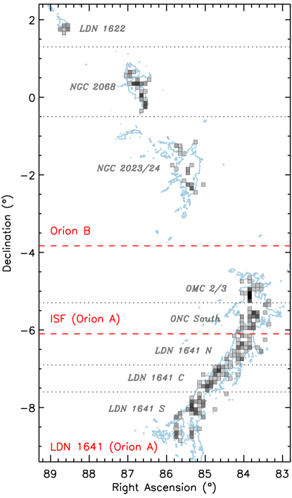
Figure 1: Locations within Orion of the 410 HOPS sources. Each box covers $0.1^{\circ}\times 0.1^{\circ}$ and is shaded according to the number of HOPS sources within its bounds. The lightest boxes contain single HOPS sources, while the darkest box contains 21. Gray labels and dotted lines indicate the regions listed in Table 1, while red labels and dashed lines show how they are combined into super-regions in Section 3.2. The 1.5 Jy beam^-1 contours from the Herschel 500 µm map are shown in blue (Stutz & Kainulainen, 2015).

2.1 Mapping Procedure

The HOPS targets were divided into distinct spatial groups to optimize observing and were imaged in a series of partially overlapping square maps, either 5′ or 8′ on a side. The map centers and sizes can be found in Tables 1 and 2 of Stutz et al. (2013). We used PACS and its scan-map astronomical observing template, with the slowest allowed scan speed (20″ s^-1), to simultaneously obtain 70 µm and 160 µm images. To avoid the striping characteristic of bolometer arrays (Tegmark, 1997), we mapped each group in two orthogonal scan directions that have consecutive observation identifiers (ObsIDs). Multiple scan legs were needed to cover each group, since they are larger than the 1.75′ $\times$ 3.5′ PACS field of view. Our first imaging data were obtained for a single field on 2009 October 9 in the science demonstration phase (Fischer et al., 2010; Stanke et al., 2010), and subsequent imaging data were obtained between 2010 March 10 and 2011 September 19. In the Appendix, we present the HOPS catalog and discuss the data processing, map generation, and photometric techniques.

3 Dependence of Photometry on Evolutionary Stage and Environment

Here we examine trends in the 70 µm flux densities and the ratios of 160 µm to 70 µm flux densities of the HOPS protostars as functions of evolutionary stage and region. We use the evolutionary classes assigned by Furlan et al. (2016) based on mid-IR spectral indices and bolometric temperatures. These follow the standard scheme reviewed by Dunham et al. (2014), where protostars are classified as Class 0, Class I, or flat-spectrum. These classes approximately represent a sequence of evolutionary stages. In the Class 0 protostars, most of the mass is still expected to be in the envelope instead of the star. In contrast, the Class I protostars still have a significant envelope, but most of the mass is expected to be in the star. The flat-spectrum protostars have residual envelopes that typically exceed the masses of their disks. Class II sources are considered to be post-protostellar, although some have residual envelopes.

Since the classification is based on the SED, which may be affected by foreground reddening and the inclination of the protostar, each evolutionary stage may include objects from previous or subsequent classes. Furlan et al. (2016) used the 4.5–24 µm spectral index, which is expected to be relatively unaffected by foreground extinction compared to indices at shorter wavelengths, but they did not explicitly account for extinction in their classification. Although extinction may affect the sorting into Class II YSOs, flat-spectrum protostars, and Class I protostars, the Class 0 protostars were identified by their low $T_{\rm bol}$. As Stutz & Kainulainen (2015) showed statistically, based on the HOPS grid of SED models (Furlan et al., 2016), the rate at which Class I protostars are misclassified as Class 0 protostars due to foreground extinction is small.

Direct comparison of flux densities is valid if all sources are roughly at the same distance. Kounkel et al. (2018) find that the distances to the protostars in our study range from 417 pc at the southern end of LDN 1641 to 389 pc in the vicinity of the ONC, with NGC 2023/24 and NGC 2068 at 403 pc and 417 pc, respectively. They conclude that LDN 1622, at 345 pc, is not part of Orion B; see footnote 2 to Table 1. The ratio of the largest to the smallest distance, squared, is 0.06 in logarithmic units, or 0.16 if LDN 1622 is included. This is negligible compared to the range of flux densities considered in this paper. Including more distant Gaia stars in their analyses, subsequent researchers (Großschedl et al., 2018; Zucker et al., 2020; Rezaei Kh. et al., 2020) reported a distance of 450 pc to the southern end of LDN 1641. This would increase the ratio reported above from 0.16 to 0.23, still small compared to the differences in flux density among regions.

3.1 Trends with Evolutionary Stage

Figure 2 plots the 70 µm flux density against the 160 µm to 70 µm flux density ratio for protostars in our sample that were detected at both wavelengths. By attempting to detect artificial sources in the 70 µm images, Stutz & Kainulainen (2015) estimated that in their regions 1 and 2 (our OMC 2/3 and ONC South), more than 90% of protostars brighter than 0.12 Jy at 70 µm were detected. Elsewhere in Orion A, the limit was lower, 0.03 Jy, as expected from the reduced nebulosity. Limits have not been calculated for Orion B, but we do not expect them to be more severe than 0.12 Jy, because it has low nebulosity compared to the ONC. (The NGC 2024 H II region that covers a small fraction of the NGC 2023/24 region’s area may be an exception.) In the following analysis, we ignore all sources fainter than 0.12 Jy at 70 µm to reduce the impact of region-dependent completeness on the results.

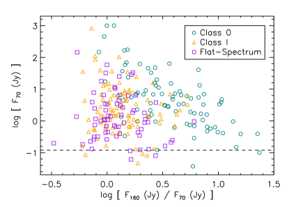
Figure 2: Plot of 70 µm flux density against 160 µm to 70 µm flux density ratio for protostars in our sample that were detected at both wavelengths. This includes 84 of 92 Class 0 protostars, 94 of 125 Class I protostars, and 69 of 102 flat-spectrum protostars. The dashed line at $F_{70}=0.12$ Jy is the 90% completeness limit calculated near the ONC by Stutz & Kainulainen (2015). Although the completeness limit is less stringent in other regions, all sources fainter than this limit are excluded from our analysis to permit region-to-region comparison.

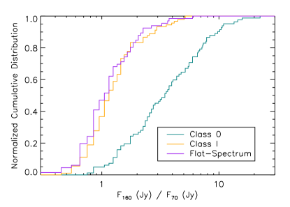
Figure 3: Cumulative distributions of the ratio of 160 µm to 70 µm flux density for protostars in each evolutionary class. We require a flux density in excess of 0.12 Jy at 70 µm and a detection at 160 µm, so the plot is based on 82 of 92 Class 0 protostars, 90 of 125 Class I protostars, and 66 of 102 flat-spectrum protostars. The Class 0 protostars are significantly redder in the far IR than protostars of the other two classes.

In Figure 2, Class 0 protostars occupy a distinct region of the space and are significantly redder than other protostars when the flux density at 70 µm is $\lesssim 10$ Jy. The decreasing color with increasing flux was predicted by synthetic photometry of a grid of protostar models in Ali et al. (2010), where, holding other parameters such as envelope density and outflow cavity opening angle constant, increasing the luminosities led to smaller 160 µm to 70 µm flux density ratios. The figure also shows that the flux density ratios of Class I and flat-spectrum protostars are indistinguishable and lack a strong dependence on flux density.

The cumulative distribution functions in Figure 3 and associated Kolmogorov-Smirnov (KS) tests confirm these class differences. The probabilities that the Class 0 flux density ratios are drawn from the same underlying distribution as the Class I and flat-spectrum flux density ratios are $1\times 10^{-14}$ and $1\times 10^{-13}$, respectively. Because the probabilities are very low, we conclude that the Class 0 protostars have significantly different flux density ratios from the other classes. The KS probability that the Class I and flat-spectrum flux density ratios are drawn from the same distribution is 0.17, so these classes are indistinguishable. The general trend is not surprising, because classification by evolutionary state is based on the shape of the SED. With $T_{\rm bol}<70$ K, Class 0 SEDs peak at a range of wavelengths in the far-IR and can have a range of flux density ratios there, while the SEDs of more evolved protostars peak at shorter wavelengths and cover a narrower range of smaller far-IR flux density ratios. More remarkable is the large separation between Class 0 protostars and other protostars for this flux density ratio alone.

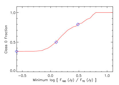
Figure 4: Fraction of protostars that are Class 0 as a function of minimum flux density ratio. When considering all 238 protostars detected in both bands that satisfy the completeness limit (see text), 34% of protostars are Class 0 (left symbol). When limiting the sample to include only those with larger flux density ratios (redder colors), an increasing fraction of protostars are Class 0. Based on the ratio of these two flux densities alone, 50% of a large sample of protostars with $\log\ [F_{160}/F_{70}]>0.10$ (in $F_{\nu}$ units; middle symbol) and 80% of such a sample with $\log\ [F_{160}/F_{70}]>0.48$ (right symbol) are likely to be Class 0.

This separation highlights the value of far-IR data for identifying the youngest, most rapidly accreting protostars. It circumvents the need to obtain data with broad wavelength coverage from multiple telescopes to calculate the usual diagnostics of bolometric temperature or submillimeter to bolometric luminosity ratio. Furthermore, the far-IR ratio is relatively insensitive to foreground extinction and the inclination of the protostar (Ali et al., 2010; Stutz & Kainulainen, 2015), factors that strongly affect the overall shape of the SED (e.g., Whitney et al., 2003; Furlan et al., 2016).

Figure 4 shows how the fraction of Class 0 protostars is higher in samples with larger 160 µm to 70 µm flux density ratios. When all protostars detected in both bands are included, the Class 0 fraction is 34%, similar to what has been found in other studies of different star-forming regions (Dunham et al., 2014), but slightly larger because we have excluded 160 µm non-detections. In a sample of protostars with $\log\ [F_{160}/F_{70}]>0.10$ (in $F_{\nu}$ units), however, 50% are likely to be Class 0. When $\log\ [F_{160}/F_{70}]>0.48$, 80% are likely to be Class 0.

3.2 Trends with Location and Environment

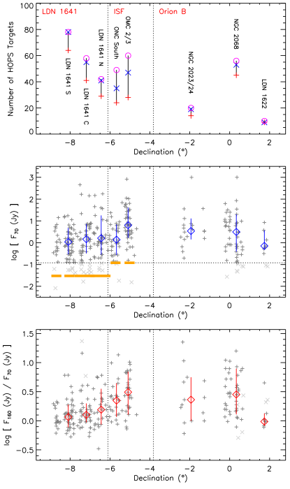
Figure 5: Properties of the HOPS targets plotted by declination. Sources are binned by the regions listed in Table 1. Top: Number of targets per region. Magenta indicates all targets that were observed, blue indicates those with 70 µm detections, and red indicates those with 160 µm detections (which are also 70 µm detections in 253 of 254 cases). Middle: Flux densities at 70 µm. The thick orange lines show the completeness limits determined by Stutz & Kainulainen (2015). Sources below the dotted line are ignored in the analysis to reduce the effect of varying completeness. Bottom: Ratios of 160 µm to 70 µm flux densities. Sources that were excluded from the analysis in the middle panel are marked with $\times$ symbols and also excluded in the calculation of statistics shown here. In the bottom two panels, diamonds mark the median in each region, and vertical lines extend over the middle 68% of the data in each region.

The top panel of Figure 5 shows how the numbers of HOPS targets detected at 70 µm and 160 µm depend on their location within Orion. (In this figure, we consider all targets, including those that are less likely to be protostars.) Declination is plotted as a proxy for region; see Table 1 for the declinations covered by each region. The number of targets observed per region varies between ten in LDN 1622 and 78 in LDN 1641 S, while the fraction detected at 70 µm ranges from 71% in ONC South to 100% in LDN 1641 S. The fraction detected at 160 µm ranges from 47% in OMC 2/3 to 90% in LDN 1622. At both wavelengths, the detection fractions are much lower in the two regions on the periphery of the ONC (ONC South and OMC 2/3), consistent with the finding of Stutz & Kainulainen (2015) that brighter nebulosity makes far-IR detections of protostars more challenging.

The lower two panels in Figure 5 show the distributions of 70 µm flux densities and 160 µm to 70 µm flux density ratios for each region. The middle panel shows the effect on the sample of the completeness cut discussed above. Of the 337 detections at 70 µm, Furlan et al. (2016) classified 319 as protostars, so the distribution of HOPS protostars is similar to what is plotted. Of the 254 detections at 160 µm, 253 are also detected at 70 µm.

In Orion A (the five southernmost regions in Figure 5), the brightest and reddest protostars are in OMC 2/3. Both the 70 µm flux densities and the 160 µm to 70 µm flux density ratios decrease from north to south. In Orion B, the flux density ratios and flux densities for NGC 2023/24 and NGC 2068 are similar to those in the northernmost reaches of Orion A. The flux density ratios and flux densities for LDN 1622 are among the lowest observed, although analysis in this region is subject to a severely limited sample size.

For better statistics in the remaining analysis, we combine the regions listed in Table 1 into three super-regions. LDN 1622, NGC 2028, and NGC 2023/24 are combined into “Orion B.” OMC 2/3 and ONC South are combined into “ISF.” All of the LDN 1641 sub-regions are combined. We also focus strictly on the sources classified as protostars.

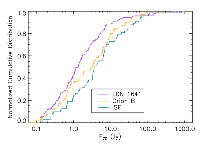
Figure 6: Cumulative distributions of the 70 µm flux density for protostars in each super-region. We require a flux density in excess of 0.12 Jy at 70 µm, so the plot is based on 146 of 165 protostars in LDN 1641, 71 of 78 protostars in Orion B, and 73 of 76 protostars in the ISF. The ISF protostars are marginally brighter at 70 µm than the Orion B protostars, which are in turn brighter than the LDN 1641 protostars.

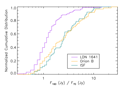
Figure 7: Cumulative distributions of the ratio of 160 µm to 70 µm flux density for protostars in each super-region. We require a flux density in excess of 0.12 Jy at 70 µm and a detection at 160 µm, so the plot is based on 126 of 165 protostars in LDN 1641, 61 of 78 protostars in Orion B, and 51 of 76 protostars in the ISF. The ISF and Orion B protostars have similar colors and are redder than the LDN 1641 protostars.

Figure 6 shows cumulative distributions of the 70 µm flux density for protostars in each super-region. It shows that the ISF protostars are marginally brighter at 70 µm than the Orion B protostars, which are in turn brighter than the LDN 1641 protostars. The KS probabilities that the ISF flux densities are drawn from the same underlying distribution as the Orion B and LDN 1641 flux densities are 0.29 and $3.5\times 10^{-5}$, respectively. The KS probability that the Orion B and LDN 1641 flux densities come from the same distribution is $8.8\times 10^{-3}$.

Figure 7 shows cumulative distributions of the ratio of 160 µm to 70 µm flux density for protostars in each super-region. It shows that the ISF and Orion B protostars are redder than the LDN 1641 protostars. The KS probability that the ISF and Orion B flux density ratios are drawn from the same underlying distribution is 0.72. The KS probabilities that the LDN 1641 ratios are drawn from the same underlying distribution as the ISF and Orion B ratios are $4.4\times 10^{-7}$ and $1.3\times 10^{-5}$, respectively. These trends clearly demonstrate systematic variations in the properties of protostars across the Orion clouds. Most significantly, the far-IR colors of the protostars are redder for the ISF and Orion B regions than for the LDN 1641 region. Furthermore, the 70 µm flux distributions for all three clouds are different, with the ISF containing the brightest protostars, then Orion B, then LDN 1641. Of particular note is the systematic variation of the protostellar properties across the Orion A cloud.

4 Discussion

The parameter most likely to be responsible for the systematic variation in colors is envelope density. This can be established by reviewing the findings of Ali et al. (2010), who used a grid of radiative transfer models (later expanded and used to fit the SEDs of the HOPS protostars by Furlan et al. 2016) to examine how protostellar properties affect the Herschel colors. Important properties that determine the colors are the inclination of the outflow cavity, the opening angle of the outflow cavity, the luminosity of the protostar, and the density of the envelope (usually stated at 1 AU or 1000 AU based on models that assume a radius^-3/2 density law; see Furlan et al. 2016).

Examining these four properties, systematic variations in inclination are unlikely, since we expect the protostars to be randomly oriented. Outflow cavity sizes may vary systematically with region; however, the cavity opening angle has a relatively small effect on the far-IR colors. As luminosity increases, Ali et al. (2010) showed that the 70 µm flux density increases while the 160 µm to 70 µm flux density ratio decreases, the opposite of the correlations seen in Figures 5, 6, and 7. This suggests that the changing colors trace systematic changes in the distribution of envelope densities across the Orion clouds.

Within Orion A, flux densities and flux density ratios increase from south to north, showing an environmental dependence, with location as a proxy for environment. Similarly, Stutz & Kainulainen (2015) found a systematic variation in the ratio of Class 0 to Class I protostars across the Orion A cloud, with the highest ratio toward the OMC 2/3 and ONC South regions. Stutz & Kainulainen (2015) and Stutz & Gould (2016) demonstrated that, along with a larger Class 0 fraction, the ISF has higher column densities than LDN 1641. Stutz & Gould (2016) and González Lobos & Stutz (2019) further showed that the ISF has both higher densities and distinct gas kinematics compared to LDN 1641. Carpenter (2000), Megeath et al. (2016), and Stutz (2018) showed that the ONC has the highest stellar densities in Orion A. Furthermore, Pokhrel et al. (2020) found that the gas and stellar densities in Orion A are strongly correlated.

The Orion B protostars are similar to those in the ISF in the distribution of their far-IR colors. Orion B, specifically NGC 2068, contains an excess of Herschel-detected protostars that are too deeply embedded to have been detected with Spitzer (Stutz et al., 2013) and have morphological evidence of youth (Karnath et al., 2020). Like the ISF, Orion B is dominated by young stellar clusters, in contrast to the young stars in LDN 1641, which are primarily found in smaller groups or in relative isolation (Megeath et al., 2016). Also like the ISF, the Orion B cloud may be directly influenced by the massive stars in the Orion OB1 association (e.g., Brown et al. 1994).

One explanation for the systematic changes from region to region in the typical envelope densities is that the star formation rate (SFR) is varying with time in different ways across the Orion clouds. Regions with a rising SFR will show a higher ratio of younger (Class 0) to older (Class I) protostars and, therefore, higher median envelope densities than regions with a falling SFR. For example, if the Class 0 lifetime is 0.15 Myr (Dunham et al., 2014), a region with a constant SFR would have a Class 0 fraction of 30% at 0.5 Myr (see Fig. 3 of Stutz & Kainulainen 2015). In contrast, a region with a star formation episode that started 0.5 Myr ago and an SFR that increased linearly with time would have a Class 0 fraction of 51%. The exact fraction is determined by the time since the onset of star formation and how the SFR varies with time. Given the unusually low star formation efficiency in Orion B (Megeath et al., 2016) and the high fraction of very young protostars there (Stutz & Gould, 2016; Karnath et al., 2020), the Orion B cloud may be undergoing a rapid rise in the SFR. The OMC 2/3 region in the ISF, which is rich in young protostars, may also be undergoing such a rise.

Alternatively, regions with overall higher gas density may have systematically more massive envelopes that have shorter free-fall times and collapse to form stars more rapidly (Kryukova et al., 2012; Dunham et al., 2014). This inference is consistent with the distributions of bolometric temperatures and envelope masses for these different regions as found in an analysis of the HOPS protostars by Fischer et al. (2017). In contrast to the previous scenario, the SFR in this case is similar from region to region, but the resulting protostellar envelopes are more massive in regions with higher Class 0 fractions. Since the ISF region is known to have the highest gas densities in the Orion A cloud (Wilson et al., 1999; Stutz & Kainulainen, 2015; Stutz & Gould, 2016; Hacar et al., 2020), this could explain the high median envelope densities in the ISF. It is also possible that both effects are operating, with, for example, the rise in the SFR resulting in the high envelope densities in Orion B and the overall high gas densities resulting in the high envelope densities in the ISF. In either case, the variations demonstrate that the properties of protostars are correlated with environmental conditions and can potentially be used as tracers of the star formation history (the first scenario) or the effect of environment on the star formation process (the second scenario).

5 Conclusions

We described the far-IR photometry of Orion protostars obtained as part of the Herschel key program HOPS. The ratio of 160 µm to 70 µm flux densities is an effective means of classifying protostars. Class 0 protostars occupy a distinct region of the 70 µm flux versus 160 µm to 70 µm flux ratio diagram and show an inverse correlation between the two quantities; i.e., fainter Class 0 protostars are redder. More evolved protostars lack such a correlation. Additionally, Class 0 protostars have significantly larger 160 µm to 70 µm flux density ratios than Class I and flat-spectrum protostars, which are statistically indistinguishable at these wavelengths. This shows that Class 0 protostars are fundamentally different from their more evolved counterparts. In a population of protostars, 80% of those with $\log\ [F_{160}/F_{70}]>0.48$ (in $F_{\nu}$ units) are likely to be Class 0. This finding circumvents the need for large multiwavelength datasets to reliably identify the most embedded protostars.

We found that redder and brighter protostars are preferentially located in the ISF and the two southern regions of Orion B relative to LDN 1641. This is consistent with the work of others, who show larger Class 0 / Class I fractions in those regions as well as greater gas and stellar densities. These traits can be interpreted as evidence for increasing star formation rates in the ISF and Orion B or as a tendency for more massive envelopes to be inherited from denser birth environments.

Appendix A The HOPS Catalog

The list of HOPS targets appears in Table 2. For completeness, we include all 410 objects with HOPS identifiers, whether or not these were actually observed with Herschel or classified as protostars. Furlan et al. (2016) identify the 330 HOPS sources that have high probabilities of being YSOs, including 319 that are likely Class 0, Class I, or flat-spectrum protostars.

In Table 2, column 1 lists the HOPS number, and columns 2 and 3 give coordinates. Column 4 identifies the region within the Orion A and B clouds to which the HOPS source belongs, defined in Table 1. Column 5 lists the date on which the group containing the source was observed. Column 6 gives the Herschel ObsIDs, two per group as described in Section 2.1, and column 7 lists the group number. Since sources can appear in more than one group, we list the one for which the source position had the longest exposure time. (Sources mapped in ObsIDs 1342205228–29 were also mapped with shorter exposure times in 1342205230–31, designed to mitigate saturation in OMC 2/3.) Columns 8 through 10 pertain to the 70 µm photometry, giving the flux, uncertainty, and photometric technique. The techniques are discussed in Appendix C; entries indicate whether the measurement is from aperture photometry (A; Appendix C.1) or PSF photometry (P; Appendix C.2) or the source was not detected (X). Upper limits are given for some sources that were not detected. Columns 11 through 13 show the same information for the 160 µm photometry. Sources with no ObsIDs were not covered by the maps or are duplicates of other sources.

Table 2: HOPS Sources

	R.A.	Decl.		Obs. Date			70 µm			160 µm
HOPS	(∘)	(∘)	Region	(UT)	ObsID	Group	Flux (Jy)	Unc. (Jy)	Type	Flux (Jy)	Unc. (Jy)	Type
000	88.6171	$-$1.6264	LDN 1622	$\cdots$	$\cdots$	$\cdots$	$\cdots$	$\cdots$	$\cdots$	$\cdots$	$\cdots$	$\cdots$
001	88.5514	$-$1.7099	LDN 1622	2011 Mar 06	1342215365$-$66	000	3.697e$+$00	1.850e$-$01	A	3.836e$+$00	2.039e$-$01	A
002	88.5380	$-$1.7144	LDN 1622	2011 Mar 06	1342215365$-$66	000	5.188e$-$01	2.617e$-$02	A	4.013e$-$01	4.013e$-$02	P
003	88.7374	$-$1.7156	LDN 1622	2011 Apr 18	1342218780$-$81	001	3.187e$-$01	1.622e$-$02	A	2.621e$-$01	1.628e$-$02	A
004	88.7240	$-$1.7861	LDN 1622	2011 Apr 18	1342218780$-$81	001	6.116e$-$01	3.083e$-$02	A	5.926e$-$01	3.290e$-$02	A
005	88.6340	$-$1.8020	LDN 1622	2011 Apr 16	1342218703$-$04	003	7.103e$-$01	3.573e$-$02	A	6.885e$-$01	4.186e$-$02	A
006	88.5767	$-$1.8176	LDN 1622	2011 Apr 16	1342218703$-$04	003	9.110e$-$02	5.523e$-$03	A	1.900e$-$01	1.900e$-$02	A
007	88.5835	$-$1.8452	LDN 1622	2011 Apr 16	1342218703$-$04	003	1.342e$+$00	6.728e$-$02	A	1.792e$+$00	9.277e$-$02	A
008	83.8880	$-$5.9851	ONC South	2011 Aug 24	1342227328$-$29	006	$\cdots$	$\cdots$	X	$\cdots$	$\cdots$	X
009	83.9550	$-$5.9843	ONC South	$\cdots$	$\cdots$	$\cdots$	$\cdots$	$\cdots$	$\cdots$	$\cdots$	$\cdots$	$\cdots$
010	83.7875	$-$5.9743	ONC South	2010 Sep 09	1342204248$-$49	005	6.823e$+$00	3.414e$-$01	A	1.770e$+$01	9.111e$-$01	A
011	83.8059	$-$5.9661	ONC South	2010 Sep 09	1342204248$-$49	005	2.357e$+$01	1.179e$+$00	A	3.641e$+$01	1.861e$+$00	A
012	83.7858	$-$5.9317	ONC South	2010 Sep 09	1342204248$-$49	005	1.556e$+$01	7.825e$-$01	A	4.172e$+$01	4.172e$+$00	P
013	83.8523	$-$5.9260	ONC South	2011 Aug 24	1342227328$-$29	006	1.122e$+$00	5.636e$-$02	A	1.071e$+$00	7.326e$-$02	A
014	84.0799	$-$5.9251	ONC South	2011 Aug 24	1342227326$-$27	007	$\cdots$	$\cdots$	X	3.626e$+$00	$\cdots$	X
015	84.0792	$-$5.9237	ONC South	2011 Aug 24	1342227326$-$27	007	2.578e$-$01	1.368e$-$02	A	2.926e$+$00	$\cdots$	X
016	83.7534	$-$5.9238	ONC South	2010 Sep 09	1342204248$-$49	005	6.854e$-$01	3.467e$-$02	A	6.470e$+$00	$\cdots$	X
017	83.7799	$-$5.8683	ONC South	2011 Mar 30	1342217446$-$47	008	6.729e$-$01	3.579e$-$02	A	5.953e$+$00	$\cdots$	X
018	83.7729	$-$5.8651	ONC South	2011 Mar 30	1342217446$-$47	008	4.268e$+$00	2.150e$-$01	A	6.307e$+$00	6.307e$-$01	P
019	83.8583	$-$5.8563	ONC South	2011 Mar 30	1342217446$-$47	008	2.470e$-$01	1.892e$-$02	A	9.535e$-$01	9.535e$-$02	P
020	83.3780	$-$5.8447	ONC South	2011 Mar 31	1342217750$-$51	009	1.373e$+$00	6.895e$-$02	A	3.261e$+$00	1.756e$-$01	A
021	84.0421	$-$5.8357	ONC South	2011 Aug 22	1342227096$-$97	010	1.185e$-$01	9.084e$-$03	A	1.376e$+$00	$\cdots$	X
022	83.7522	$-$5.8172	ONC South	2011 Mar 30	1342217446$-$47	008	1.455e$-$01	1.623e$-$02	A	6.369e$+$00	$\cdots$	X
023	84.0745	$-$5.7818	ONC South	2011 Aug 22	1342227096$-$97	010	$\cdots$	$\cdots$	X	$\cdots$	$\cdots$	X
024	83.6956	$-$5.7475	ONC South	2010 Sep 09	1342204246$-$47	012	2.908e$-$01	1.936e$-$02	A	5.810e$-$01	$\cdots$	X
025	83.8443	$-$5.7415	ONC South	2011 Aug 22	1342227098$-$99	013	$\cdots$	$\cdots$	X	$\cdots$	$\cdots$	X
026	83.8222	$-$5.7040	ONC South	2011 Aug 22	1342227098$-$99	013	1.303e$-$01	1.850e$-$02	A	2.295e$+$00	$\cdots$	X
027	84.0905	$-$5.6995	ONC South	$\cdots$	$\cdots$	$\cdots$	$\cdots$	$\cdots$	$\cdots$	$\cdots$	$\cdots$	$\cdots$
028	83.6971	$-$5.6989	ONC South	2010 Sep 09	1342204246$-$47	012	9.445e$-$01	4.860e$-$02	A	2.570e$+$00	2.570e$-$01	P
029	83.7044	$-$5.6951	ONC South	2010 Sep 09	1342204246$-$47	012	3.772e$+$00	1.890e$-$01	A	3.898e$+$00	3.898e$-$01	P
030	83.6836	$-$5.6905	ONC South	2010 Sep 09	1342204246$-$47	012	7.611e$+$00	3.810e$-$01	A	1.303e$+$01	1.303e$+$00	P
031	83.8219	$-$5.6741	ONC South	2011 Aug 22	1342227098$-$99	013	$\cdots$	$\cdots$	X	$\cdots$	$\cdots$	X
032	83.6477	$-$5.6664	ONC South	2010 Sep 09	1342204244$-$45	014	6.168e$+$00	3.098e$-$01	A	7.714e$+$00	7.714e$-$01	P
033	83.6884	$-$5.6658	ONC South	2010 Sep 09	1342204246$-$47	012	1.079e$-$01	9.161e$-$03	A	7.510e$-$01	$\cdots$	X
034	83.7954	$-$5.6585	ONC South	2010 Sep 28	1342205234$-$35	015	$\cdots$	$\cdots$	X	$\cdots$	$\cdots$	X
035	83.8331	$-$5.6503	ONC South	2010 Sep 28	1342205234$-$35	015	$\cdots$	$\cdots$	X	$\cdots$	$\cdots$	X
036	83.6101	$-$5.6279	ONC South	2010 Sep 09	1342204244$-$45	014	9.967e$-$01	5.030e$-$02	A	8.720e$-$01	8.720e$-$02	A
037	83.6986	$-$5.6237	ONC South	2010 Sep 09	1342204244$-$45	014	$\cdots$	$\cdots$	X	$\cdots$	$\cdots$	X
038	83.7697	$-$5.6201	ONC South	2010 Sep 28	1342205234$-$35	015	2.720e$-$01	2.720e$-$02	P	1.698e$+$01	$\cdots$	X
039	84.0934	$-$5.6069	ONC South	$\cdots$	$\cdots$	$\cdots$	$\cdots$	$\cdots$	$\cdots$	$\cdots$	$\cdots$	$\cdots$
040	83.7855	$-$5.5998	ONC South	2010 Sep 28	1342205234$-$35	015	3.306e$+$00	1.727e$-$01	A	1.456e$+$01	1.456e$+$00	P
041	83.6227	$-$5.5952	ONC South	2010 Sep 09	1342204244$-$45	014	4.560e$+$00	2.292e$-$01	A	1.057e$+$01	5.732e$-$01	A
042	83.7710	$-$5.5946	ONC South	2010 Sep 28	1342205234$-$35	015	1.313e$+$00	1.231e$-$01	A	2.880e$+$01	$\cdots$	X
043	83.7688	$-$5.5873	ONC South	2010 Sep 28	1342205234$-$35	015	3.253e$+$00	3.253e$-$01	P	1.717e$+$01	1.717e$+$00	P
044	83.7941	$-$5.5851	ONC South	2010 Sep 28	1342205234$-$35	015	9.560e$-$01	9.560e$-$02	P	1.300e$+$01	1.300e$+$00	A
045	83.7769	$-$5.5598	ONC South	2010 Sep 28	1342205234$-$35	015	6.547e$+$00	6.547e$-$01	P	8.528e$+$00	8.528e$-$01	A
046	83.6758	$-$5.5509	ONC South	2011 Mar 30	1342217448$-$49	016	$\cdots$	$\cdots$	X	6.326e$+$00	$\cdots$	X
047	83.4411	$-$5.5495	ONC South	2010 Sep 13	1342204433$-$34	308	1.809e$-$02	8.193e$-$03	A	4.897e$-$01	$\cdots$	X
048	83.7773	$-$5.5477	ONC South	2010 Sep 28	1342205234$-$35	015	5.667e$+$00	$\cdots$	X	$\cdots$	$\cdots$	X
049	83.7037	$-$5.5294	ONC South	2011 Mar 30	1342217448$-$49	016	6.645e$-$01	4.765e$-$02	A	6.219e$-$01	1.089e$-$01	X
050	83.6705	$-$5.5290	ONC South	2011 Mar 30	1342217448$-$49	016	9.106e$+$00	4.566e$-$01	A	2.027e$+$01	1.106e$+$00	A
051	83.8160	$-$5.5015	ONC South	2011 Mar 30	1342217450$-$51	017	$\cdots$	$\cdots$	X	$\cdots$	$\cdots$	X
052	83.8180	$-$5.4924	ONC South	2011 Mar 30	1342217450$-$51	017	$\cdots$	$\cdots$	X	$\cdots$	$\cdots$	X
053	83.4891	$-$5.3918	ONC South	2011 Mar 31	1342217752$-$53	018	6.898e$+$01	3.465e$+$00	A	1.030e$+$02	5.259e$+$00	A
054	83.3437	$-$5.3841	ONC South	$\cdots$	$\cdots$	$\cdots$	$\cdots$	$\cdots$	$\cdots$	$\cdots$	$\cdots$	$\cdots$
055	83.4754	$-$5.3638	ONC South	2011 Mar 31	1342217752$-$53	018	$\cdots$	$\cdots$	X	1.225e$+$00	1.225e$-$01	A
056	83.8311	$-$5.2591	OMC 2/3	2010 Sep 28	1342205232$-$33	200	4.724e$+$01	2.458e$+$00	A	1.275e$+$02	1.275e$+$01	P
057	83.8327	$-$5.2524	OMC 2/3	2010 Sep 28	1342205232$-$33	200	4.907e$+$00	6.584e$-$01	A	7.511e$+$01	$\cdots$	X
058	83.8271	$-$5.2273	OMC 2/3	2010 Sep 28	1342205228$-$29	130	3.456e$+$00	4.557e$-$01	A	3.805e$+$00	$\cdots$	X
059	83.8339	$-$5.2210	OMC 2/3	2010 Sep 28	1342205228$-$29	130	5.836e$+$01	3.015e$+$00	A	5.813e$+$01	5.813e$+$00	P
060	83.8472	$-$5.2008	OMC 2/3	2010 Sep 28	1342205228$-$29	130	5.830e$+$01	2.942e$+$00	A	8.457e$+$01	8.457e$+$00	A
061	83.3580	$-$5.2007	OMC 2/3	$\cdots$	$\cdots$	$\cdots$	$\cdots$	$\cdots$	$\cdots$	$\cdots$	$\cdots$	$\cdots$
062	83.8524	$-$5.1916	OMC 2/3	2010 Sep 28	1342205228$-$29	130	$\cdots$	$\cdots$	X	4.395e$+$01	$\cdots$	X
063	83.8538	$-$5.1671	OMC 2/3	2010 Sep 28	1342205228$-$29	130	$\cdots$	$\cdots$	X	$\cdots$	$\cdots$	X
064	83.8625	$-$5.1650	OMC 2/3	2010 Sep 28	1342205228$-$29	130	$\cdots$	$\cdots$	X	$\cdots$	$\cdots$	X
065	83.8398	$-$5.1608	OMC 2/3	2010 Sep 28	1342205228$-$29	130	4.812e$-$01	8.142e$-$02	A	2.835e$+$01	$\cdots$	X
066	83.8619	$-$5.1568	OMC 2/3	2010 Sep 28	1342205228$-$29	130	2.719e$+$01	2.719e$+$00	P	3.246e$+$02	$\cdots$	X
067	83.8445	$-$5.1428	OMC 2/3	2010 Sep 28	1342205228$-$29	130	$\cdots$	$\cdots$	X	$\cdots$	$\cdots$	X
068	83.8513	$-$5.1418	OMC 2/3	2010 Sep 28	1342205228$-$29	130	6.959e$+$00	3.723e$-$01	A	2.551e$+$01	2.551e$+$00	A
069	83.8551	$-$5.1400	OMC 2/3	2010 Sep 28	1342205228$-$29	130	$\cdots$	$\cdots$	X	1.558e$+$01	$\cdots$	X
070	83.8434	$-$5.1347	OMC 2/3	2010 Sep 28	1342205228$-$29	130	6.413e$+$00	6.413e$-$01	P	1.161e$+$01	1.161e$+$00	A
071	83.8567	$-$5.1326	OMC 2/3	2010 Sep 28	1342205228$-$29	130	1.426e$+$01	7.339e$-$01	A	4.675e$+$01	$\cdots$	X
072	83.8571	$-$5.1296	OMC 2/3	2010 Sep 28	1342205228$-$29	130	$\cdots$	$\cdots$	X	$\cdots$	$\cdots$	X
073	83.8654	$-$5.1176	OMC 2/3	2010 Sep 28	1342205228$-$29	130	1.672e$+$00	1.251e$-$01	A	1.168e$+$01	1.168e$+$00	A
074	83.8536	$-$5.1059	OMC 2/3	2010 Sep 28	1342205228$-$29	130	1.013e$+$00	1.014e$-$01	A	2.384e$+$01	$\cdots$	X
075	83.8611	$-$5.1029	OMC 2/3	2010 Sep 28	1342205228$-$29	130	7.029e$+$00	3.768e$-$01	A	2.186e$+$01	2.186e$+$00	P
076	83.8573	$-$5.0994	OMC 2/3	2010 Sep 28	1342205228$-$29	130	2.163e$+$00	2.163e$-$01	P	9.743e$+$00	9.743e$-$01	A
077	83.8814	$-$5.0965	OMC 2/3	2010 Sep 28	1342205228$-$29	130	8.871e$+$00	4.528e$-$01	A	3.405e$+$01	$\cdots$	X
078	83.8576	$-$5.0955	OMC 2/3	2010 Sep 28	1342205228$-$29	130	1.509e$+$01	7.644e$-$01	A	5.674e$+$01	5.674e$+$00	P
079	83.8662	$-$5.0934	OMC 2/3	2010 Sep 28	1342205228$-$29	130	$\cdots$	$\cdots$	X	$\cdots$	$\cdots$	X
080	83.8549	$-$5.0860	OMC 2/3	2010 Sep 28	1342205228$-$29	130	1.555e$-$01	2.513e$-$02	A	$\cdots$	$\cdots$	X
081	83.8665	$-$5.0828	OMC 2/3	2010 Sep 28	1342205228$-$29	130	1.989e$+$00	1.071e$-$01	A	8.245e$+$00	8.245e$-$01	A
082	83.8322	$-$5.0818	OMC 2/3	2010 Sep 28	1342205228$-$29	130	3.775e$+$00	3.775e$-$01	P	1.038e$+$01	1.038e$+$00	A
083	83.9822	$-$5.0771	OMC 2/3	$\cdots$	$\cdots$	$\cdots$	$\cdots$	$\cdots$	$\cdots$	$\cdots$	$\cdots$	$\cdots$
084	83.8607	$-$5.0653	OMC 2/3	2010 Sep 10	1342204250$-$51	019	1.035e$+$02	5.191e$+$00	A	1.323e$+$02	7.120e$+$00	A
085	83.8674	$-$5.0614	OMC 2/3	2010 Sep 10	1342204250$-$51	019	2.896e$+$01	1.466e$+$00	A	4.799e$+$01	4.799e$+$00	P
086	83.8485	$-$5.0278	OMC 2/3	2010 Sep 10	1342204250$-$51	019	6.099e$+$00	6.099e$-$01	P	1.930e$+$01	$\cdots$	X
087	83.8478	$-$5.0246	OMC 2/3	2010 Sep 10	1342204250$-$51	019	6.356e$+$01	6.356e$+$00	P	2.305e$+$02	2.305e$+$01	P
088	83.8435	$-$5.0206	OMC 2/3	2010 Sep 10	1342204250$-$51	019	3.283e$+$01	1.648e$+$00	A	8.160e$+$01	8.160e$+$00	P
089	83.8332	$-$5.0174	OMC 2/3	2010 Sep 10	1342204250$-$51	019	3.341e$+$00	2.079e$-$01	A	2.965e$+$01	$\cdots$	X
090	83.8936	$-$5.0145	OMC 2/3	2010 Sep 10	1342204250$-$51	019	2.368e$+$00	1.196e$-$01	A	4.160e$-$01	$\cdots$	X
091	83.8288	$-$5.0141	OMC 2/3	2010 Sep 10	1342204250$-$51	019	3.353e$+$00	3.353e$-$01	P	3.428e$+$01	3.428e$+$00	P
092	83.8263	$-$5.0092	OMC 2/3	2010 Sep 10	1342204250$-$51	019	3.297e$+$01	1.654e$+$00	A	5.625e$+$01	5.625e$+$00	P
093	83.8126	$-$5.0023	OMC 2/3	2010 Sep 10	1342204250$-$51	019	2.491e$+$00	1.580e$-$01	A	4.897e$+$01	$\cdots$	X
094	83.8173	$-$5.0006	OMC 2/3	2010 Sep 10	1342204250$-$51	019	6.338e$+$00	3.446e$-$01	A	3.277e$+$01	3.277e$+$00	P
095	83.8925	$-$4.9978	OMC 2/3	2010 Sep 10	1342204250$-$51	019	6.320e$-$01	6.320e$-$02	P	5.901e$+$00	5.901e$-$01	P
096	83.8738	$-$4.9802	OMC 2/3	2010 Sep 10	1342204250$-$51	019	6.898e$+$00	3.536e$-$01	A	5.125e$+$01	2.802e$+$00	A
097	83.8704	$-$4.9608	OMC 2/3	2010 Sep 10	1342204250$-$51	019	$\cdots$	$\cdots$	X	$\cdots$	$\cdots$	X
098	83.8305	$-$4.9291	OMC 2/3	2011 Mar 31	1342217758$-$59	020	1.648e$+$00	1.648e$-$01	P	4.644e$+$00	$\cdots$	X
099	83.6229	$-$4.9252	OMC 2/3	2011 Mar 31	1342217754$-$55	021	3.595e$+$00	1.801e$-$01	A	8.851e$+$00	4.621e$-$01	A
100	83.5891	$-$4.9208	OMC 2/3	2011 Mar 31	1342217754$-$55	021	1.531e$-$02	5.899e$-$03	A	2.330e$+$00	$\cdots$	X
101	83.7843	$-$4.9027	OMC 2/3	2011 Mar 31	1342217758$-$59	020	2.842e$+$00	2.842e$-$01	A	4.811e$+$01	$\cdots$	X
102	83.6466	$-$4.8716	OMC 2/3	2011 Mar 31	1342217754$-$55	021	6.403e$-$01	3.472e$-$02	A	4.676e$+$00	$\cdots$	X
103	83.5508	$-$4.8353	OMC 2/3	2011 Mar 31	1342217754$-$55	021	$\cdots$	$\cdots$	X	$\cdots$	$\cdots$	X
104	83.7782	$-$4.8338	OMC 2/3	2011 Mar 31	1342217758$-$59	020	$\cdots$	$\cdots$	X	$\cdots$	$\cdots$	X
105	83.8845	$-$4.7801	OMC 2/3	2010 Mar 10	1342191970$-$71	306	2.590e$-$01	1.789e$-$02	A	1.133e$+$00	$\cdots$	X
106	84.0518	$-$4.7544	OMC 2/3	$\cdots$	$\cdots$	$\cdots$	$\cdots$	$\cdots$	$\cdots$	$\cdots$	$\cdots$	$\cdots$
107	83.8473	$-$4.6696	OMC 2/3	2011 Mar 31	1342217756$-$57	024	4.368e$+$00	2.290e$-$01	A	5.556e$+$00	5.364e$-$01	A
108	83.8628	$-$5.1668	OMC 2/3	2010 Sep 28	1342205228$-$29	130	4.081e$+$01	4.081e$+$00	P	2.702e$+$02	2.702e$+$01	P
2109	$\cdots$	$\cdots$	$\cdots$	$\cdots$	$\cdots$	$\cdots$	$\cdots$	$\cdots$	$\cdots$	$\cdots$	$\cdots$	$\cdots$
110	84.0093	$-$5.0472	OMC 2/3	$\cdots$	$\cdots$	$\cdots$	$\cdots$	$\cdots$	$\cdots$	$\cdots$	$\cdots$	$\cdots$
2111	$\cdots$	$\cdots$	$\cdots$	$\cdots$	$\cdots$	$\cdots$	$\cdots$	$\cdots$	$\cdots$	$\cdots$	$\cdots$	$\cdots$
112	85.1833	$-$7.3786	LDN 1641 C	$\cdots$	$\cdots$	$\cdots$	$\cdots$	$\cdots$	$\cdots$	$\cdots$	$\cdots$	$\cdots$
113	84.9922	$-$7.4448	LDN 1641 C	2011 Mar 07	1342215589$-$90	025	5.930e$-$02	3.907e$-$03	A	2.560e$-$01	$\cdots$	X
114	85.0057	$-$7.4274	LDN 1641 C	2011 Mar 07	1342215589$-$90	025	1.114e$-$01	6.204e$-$03	A	1.236e$-$01	1.310e$-$02	X
115	84.9854	$-$7.4310	LDN 1641 C	2011 Mar 07	1342215589$-$90	025	2.601e$-$01	1.364e$-$02	A	2.580e$-$01	2.580e$-$02	P
116	84.9912	$-$7.4203	LDN 1641 C	2011 Mar 07	1342215589$-$90	025	3.281e$-$01	1.714e$-$02	A	3.980e$-$01	3.980e$-$02	P
117	84.9810	$-$7.4054	LDN 1641 C	2011 Mar 07	1342215589$-$90	025	1.226e$-$01	7.029e$-$03	A	2.430e$-$01	2.430e$-$02	P
118	84.9774	$-$7.4041	LDN 1641 C	2011 Mar 07	1342215589$-$90	025	1.293e$-$01	7.438e$-$03	A	7.770e$-$02	7.770e$-$03	X
119	84.9610	$-$7.3918	LDN 1641 C	2011 Mar 07	1342215589$-$90	025	7.459e$-$01	3.751e$-$02	A	5.780e$-$01	5.780e$-$02	P
120	84.8930	$-$7.4365	LDN 1641 C	2011 Mar 07	1342215589$-$90	025	1.625e$-$01	8.558e$-$03	A	5.390e$-$01	5.390e$-$02	P
121	84.8904	$-$7.3839	LDN 1641 C	2011 Apr 17	1342218729$-$30	026	4.268e$-$01	2.161e$-$02	A	2.877e$+$00	$\cdots$	X
122	84.9380	$-$7.3204	LDN 1641 C	2011 Mar 07	1342215589$-$90	025	4.470e$-$02	8.940e$-$03	A	$\cdots$	$\cdots$	X
123	84.8888	$-$7.3826	LDN 1641 C	2011 Aug 22	1342227084$-$85	313	6.141e$-$01	3.105e$-$02	A	2.471e$+$00	1.267e$-$01	A
124	84.8333	$-$7.4364	LDN 1641 C	2011 Apr 17	1342218729$-$30	026	1.650e$+$02	8.255e$+$00	A	2.361e$+$02	1.199e$+$01	A
125	84.8317	$-$7.4386	LDN 1641 C	2011 Apr 17	1342218729$-$30	026	2.158e$+$01	2.158e$+$00	P	$\cdots$	$\cdots$	X
126	85.0408	$-$7.1650	LDN 1641 C	$\cdots$	$\cdots$	$\cdots$	$\cdots$	$\cdots$	$\cdots$	$\cdots$	$\cdots$	$\cdots$
127	84.7539	$-$7.3396	LDN 1641 C	2011 Aug 22	1342227086$-$87	028	7.545e$-$01	3.793e$-$02	A	1.274e$+$00	7.042e$-$02	A
128	84.7167	$-$7.3517	LDN 1641 C	2011 Aug 22	1342227086$-$87	028	3.980e$-$01	3.980e$-$02	P	5.170e$-$01	5.170e$-$02	P
129	84.7994	$-$7.1764	LDN 1641 C	2010 Sep 10	1342204252$-$53	029	3.491e$+$00	1.748e$-$01	A	4.271e$+$00	4.271e$-$01	P
130	84.7623	$-$7.2145	LDN 1641 C	2010 Sep 10	1342204252$-$53	029	2.169e$+$00	1.086e$-$01	A	2.455e$+$00	1.312e$-$01	A
131	84.7815	$-$7.1811	LDN 1641 C	2010 Sep 10	1342204252$-$53	029	3.859e$-$01	2.018e$-$02	A	4.890e$-$01	4.890e$-$02	A
132	84.7723	$-$7.1848	LDN 1641 C	2010 Sep 10	1342204252$-$53	029	6.776e$-$01	3.456e$-$02	A	6.670e$-$01	6.670e$-$02	A
133	84.7743	$-$7.1776	LDN 1641 C	2010 Sep 10	1342204252$-$53	029	6.977e$+$00	3.492e$-$01	A	9.369e$+$00	4.818e$-$01	A
134	84.6783	$-$7.2122	LDN 1641 C	2010 Sep 10	1342204254$-$55	030	3.447e$+$00	1.726e$-$01	A	3.285e$+$00	1.723e$-$01	A
135	84.6888	$-$7.1822	LDN 1641 C	2010 Sep 10	1342204254$-$55	030	2.362e$+$00	1.183e$-$01	A	2.529e$+$00	1.331e$-$01	A
136	84.6939	$-$7.0937	LDN 1641 C	2010 Sep 28	1342205242$-$43	312	1.670e$+$00	8.378e$-$02	A	2.108e$+$00	1.148e$-$01	P
137	84.7248	$-$7.0426	LDN 1641 C	2010 Sep 10	1342204256$-$57	031	3.720e$-$02	2.813e$-$03	A	2.020e$-$01	$\cdots$	X
138	84.7014	$-$7.0454	LDN 1641 C	2010 Sep 10	1342204256$-$57	031	5.214e$-$02	4.374e$-$03	A	1.350e$+$00	$\cdots$	X
139	84.7067	$-$7.0216	LDN 1641 C	2010 Sep 10	1342204256$-$57	031	6.455e$+$00	3.230e$-$01	A	7.361e$+$00	3.906e$-$01	A
140	84.6928	$-$7.0315	LDN 1641 C	2010 Sep 10	1342204256$-$57	031	1.120e$+$00	5.636e$-$02	A	1.938e$+$00	1.938e$-$01	P
141	84.7001	$-$7.0137	LDN 1641 C	2010 Sep 10	1342204256$-$57	031	1.041e$-$01	7.545e$-$03	A	3.070e$-$01	$\cdots$	X
142	84.6990	$-$7.0075	LDN 1641 C	2010 Sep 10	1342204256$-$57	031	7.399e$-$02	6.101e$-$03	A	9.850e$-$01	$\cdots$	X
143	84.6924	$-$7.0135	LDN 1641 C	2010 Sep 10	1342204256$-$57	031	5.385e$+$00	2.713e$-$01	A	6.903e$+$00	6.903e$-$01	A
144	84.6876	$-$7.0171	LDN 1641 C	2010 Sep 10	1342204256$-$57	031	4.842e$+$00	4.842e$-$01	P	1.365e$+$01	1.365e$+$00	X
145	84.6827	$-$7.0203	LDN 1641 C	2010 Sep 10	1342204256$-$57	031	4.303e$+$00	2.158e$-$01	A	2.703e$+$00	2.703e$-$01	P
146	84.6840	$-$7.0112	LDN 1641 C	2010 Sep 10	1342204256$-$57	031	$\cdots$	$\cdots$	X	3.467e$+$00	$\cdots$	X
147	84.7292	$-$6.9385	LDN 1641 C	2010 Sep 10	1342204256$-$57	031	4.460e$-$02	8.920e$-$03	A	3.230e$-$02	4.818e$-$03	X
148	84.6646	$-$6.9918	LDN 1641 C	2010 Sep 10	1342204256$-$57	031	5.535e$-$01	2.794e$-$02	A	4.190e$-$01	4.190e$-$02	P
149	84.6687	$-$6.9727	LDN 1641 C	2010 Sep 10	1342204256$-$57	031	7.770e$+$00	3.888e$-$01	A	5.883e$+$00	3.129e$-$01	A
150	84.5314	$-$7.1414	LDN 1641 C	2011 Aug 21	1342227045$-$46	032	6.185e$+$00	3.096e$-$01	A	9.578e$+$00	4.930e$-$01	A
151	84.6787	$-$6.9447	LDN 1641 C	2010 Sep 10	1342204256$-$57	031	$\cdots$	$\cdots$	X	$\cdots$	$\cdots$	X
152	84.4948	$-$7.1237	LDN 1641 C	2011 Aug 21	1342227045$-$46	032	1.325e$+$00	6.653e$-$02	A	3.144e$+$00	3.144e$-$01	P
153	84.4875	$-$7.1157	LDN 1641 C	2011 Aug 21	1342227045$-$46	032	7.248e$+$00	3.627e$-$01	A	2.956e$+$01	1.496e$+$00	A
154	84.5837	$-$6.9847	LDN 1641 C	2011 Sep 04	1342228171$-$72	033	1.667e$-$01	1.035e$-$02	A	1.630e$-$01	1.630e$-$02	A
155	84.3160	$-$7.2972	LDN 1641 C	$\cdots$	$\cdots$	$\cdots$	$\cdots$	$\cdots$	$\cdots$	$\cdots$	$\cdots$	$\cdots$
156	84.5142	$-$6.9711	LDN 1641 C	2010 Sep 28	1342205240$-$41	034	6.727e$-$01	3.384e$-$02	A	1.050e$+$00	1.050e$-$01	P
157	84.4857	$-$6.9442	LDN 1641 C	2010 Sep 28	1342205240$-$41	034	7.617e$+$00	3.810e$-$01	A	1.106e$+$01	5.599e$-$01	A
158	84.3519	$-$6.9758	LDN 1641 C	2011 Aug 24	1342227314$-$15	035	1.449e$+$00	7.266e$-$02	A	1.481e$+$00	1.481e$-$01	P
159	84.4739	$-$6.7880	LDN 1641 N	2011 Aug 22	1342227088$-$89	036	2.273e$-$01	1.165e$-$02	A	1.610e$-$01	1.610e$-$02	A
160	84.4627	$-$6.7890	LDN 1641 N	2011 Aug 22	1342227088$-$89	036	2.849e$+$00	1.428e$-$01	A	3.859e$+$00	3.859e$-$01	P
161	84.1448	$-$7.1871	LDN 1641 C	$\cdots$	$\cdots$	$\cdots$	$\cdots$	$\cdots$	$\cdots$	$\cdots$	$\cdots$	$\cdots$
162	84.1291	$-$6.8780	LDN 1641 N	$\cdots$	$\cdots$	$\cdots$	$\cdots$	$\cdots$	$\cdots$	$\cdots$	$\cdots$	$\cdots$
163	84.3220	$-$6.6051	LDN 1641 N	2011 Aug 22	1342227090$-$91	037	8.785e$-$01	4.416e$-$02	A	7.654e$-$01	4.306e$-$02	A
164	84.2519	$-$6.6196	LDN 1641 N	2011 Aug 22	1342227090$-$91	037	7.383e$-$01	3.717e$-$02	A	4.096e$+$00	2.305e$-$01	A
165	84.0981	$-$6.7707	LDN 1641 N	2010 Sep 28	1342205238$-$39	038	2.555e$+$00	2.555e$-$01	P	7.338e$+$01	$\cdots$	X
166	84.1047	$-$6.7450	LDN 1641 N	2010 Sep 28	1342205238$-$39	038	1.776e$+$01	8.888e$-$01	A	1.575e$+$01	8.203e$-$01	A
167	84.0825	$-$6.7669	LDN 1641 N	2010 Sep 28	1342205238$-$39	038	2.026e$-$01	1.533e$-$02	A	4.005e$+$00	$\cdots$	X
168	84.0789	$-$6.7563	LDN 1641 N	2010 Sep 28	1342205238$-$39	038	1.469e$+$02	7.346e$+$00	A	1.238e$+$02	6.289e$+$00	A
169	84.1505	$-$6.6478	LDN 1641 N	2011 Aug 22	1342227094$-$95	040	5.091e$+$00	2.548e$-$01	A	2.884e$+$01	1.461e$+$00	A
170	84.1722	$-$6.5667	LDN 1641 N	2011 Aug 22	1342227092$-$93	039	1.148e$+$00	5.787e$-$02	A	9.046e$-$01	6.247e$-$02	A
171	84.0717	$-$6.6338	LDN 1641 N	2011 Aug 22	1342227094$-$95	040	4.437e$+$00	2.223e$-$01	A	6.196e$+$00	6.196e$-$01	P
172	84.0810	$-$6.4852	LDN 1641 N	2011 Aug 24	1342227316$-$17	041	1.043e$+$00	1.043e$-$01	P	1.975e$+$00	1.975e$-$01	P
173	84.1085	$-$6.4181	LDN 1641 N	2010 Sep 28	1342205236$-$37	042	2.151e$+$00	2.151e$-$01	P	5.255e$+$00	5.255e$-$01	P
174	84.1077	$-$6.4163	LDN 1641 N	2010 Sep 28	1342205236$-$37	042	1.625e$+$00	1.625e$-$01	P	7.935e$+$00	$\cdots$	X
175	84.1003	$-$6.4153	LDN 1641 N	2010 Sep 28	1342205236$-$37	042	2.858e$-$01	2.858e$-$02	A	8.795e$+$00	$\cdots$	X
176	84.0983	$-$6.4143	LDN 1641 N	2010 Sep 28	1342205236$-$37	042	9.470e$-$01	9.470e$-$02	P	5.730e$+$00	5.730e$-$01	P
177	83.9584	$-$6.5815	LDN 1641 N	2011 Aug 24	1342227310$-$11	043	1.093e$+$00	5.500e$-$02	A	1.166e$+$00	1.166e$-$01	P
178	84.1025	$-$6.3781	LDN 1641 N	2010 Sep 28	1342205236$-$37	042	3.649e$+$01	1.826e$+$00	A	4.020e$+$01	2.106e$+$00	A
179	84.0910	$-$6.3916	LDN 1641 N	2010 Sep 28	1342205236$-$37	042	1.787e$+$00	8.984e$-$02	A	3.872e$+$00	3.872e$-$01	P
180	84.2475	$-$6.1710	LDN 1641 N	$\cdots$	$\cdots$	$\cdots$	$\cdots$	$\cdots$	$\cdots$	$\cdots$	$\cdots$	$\cdots$
181	84.0813	$-$6.3701	LDN 1641 N	2010 Sep 28	1342205236$-$37	042	1.134e$+$01	1.134e$+$00	P	$\cdots$	$\cdots$	X
182	84.0785	$-$6.3695	LDN 1641 N	2010 Sep 28	1342205236$-$37	042	1.740e$+$02	8.720e$+$00	A	2.650e$+$02	1.367e$+$01	A
183	84.0744	$-$6.3745	LDN 1641 N	2010 Sep 28	1342205236$-$37	042	9.591e$-$01	9.591e$-$02	P	$\cdots$	$\cdots$	X
184	84.0539	$-$6.3918	LDN 1641 N	2010 Sep 28	1342205236$-$37	042	2.820e$-$01	1.510e$-$02	A	6.610e$-$01	6.610e$-$02	A
185	84.1541	$-$6.2494	LDN 1641 N	2010 Sep 10	1342204258$-$59	044	1.614e$+$00	8.104e$-$02	A	6.834e$+$00	6.834e$-$01	P
186	83.9470	$-$6.4374	LDN 1641 N	2011 Mar 07	1342215593$-$94	045	1.404e$+$00	7.042e$-$02	A	2.222e$+$00	1.242e$-$01	A
187	83.9622	$-$6.3788	LDN 1641 N	2011 Mar 07	1342215593$-$94	045	5.340e$-$02	1.068e$-$02	A	$\cdots$	$\cdots$	X
188	83.8743	$-$6.4495	LDN 1641 N	2011 Mar 07	1342215593$-$94	045	3.961e$+$01	1.981e$+$00	A	3.427e$+$01	1.770e$+$00	A
189	83.8787	$-$6.4422	LDN 1641 N	2011 Mar 07	1342215593$-$94	045	1.627e$+$00	8.693e$-$02	A	4.852e$+$00	4.852e$-$01	P
190	83.8687	$-$6.4505	LDN 1641 N	2011 Mar 07	1342215593$-$94	045	2.010e$-$01	2.010e$-$02	P	5.879e$+$00	$\cdots$	X
191	84.0719	$-$6.1864	LDN 1641 N	2011 Aug 24	1342227324$-$25	047	1.011e$+$00	5.078e$-$02	A	1.570e$+$00	1.570e$-$01	P
192	84.1352	$-$6.0212	ONC South	2011 Mar 30	1342217444$-$45	048	2.151e$+$00	1.081e$-$01	A	3.745e$+$00	3.745e$-$01	P
193	84.1261	$-$6.0215	ONC South	2011 Mar 30	1342217444$-$45	048	1.456e$+$00	7.304e$-$02	A	1.707e$+$00	1.707e$-$01	P
194	83.9667	$-$6.1672	LDN 1641 N	2011 Aug 24	1342227322$-$23	049	1.042e$+$01	5.214e$-$01	A	1.229e$+$01	6.450e$-$01	A
195	84.0002	$-$6.1206	LDN 1641 N	2011 Aug 24	1342227322$-$23	049	$\cdots$	$\cdots$	X	$\cdots$	$\cdots$	X
196	83.8371	$-$6.3062	LDN 1641 N	$\cdots$	$\cdots$	$\cdots$	$\cdots$	$\cdots$	$\cdots$	$\cdots$	$\cdots$	$\cdots$
197	83.5662	$-$6.5758	LDN 1641 N	2011 Mar 31	1342217748$-$49	050	1.978e$-$01	1.032e$-$02	A	6.550e$-$02	1.309e$-$02	A
198	83.8424	$-$6.2184	LDN 1641 N	2011 Aug 24	1342227318$-$19	051	2.277e$+$00	1.143e$-$01	A	4.234e$+$00	4.234e$-$01	P
199	83.6661	$-$6.4206	LDN 1641 N	2010 Aug 26	1342203649$-$50	311	1.136e$-$01	6.183e$-$03	A	1.830e$-$01	1.830e$-$02	P
200	83.8884	$-$6.1027	LDN 1641 N	2011 Aug 24	1342227320$-$21	052	4.433e$-$01	2.247e$-$02	A	4.503e$-$01	4.503e$-$02	A
201	83.5289	$-$6.5355	LDN 1641 N	2011 Mar 31	1342217748$-$49	050	7.024e$-$02	4.970e$-$03	A	7.012e$-$01	$\cdots$	X
202	83.4330	$-$6.2295	LDN 1641 N	$\cdots$	$\cdots$	$\cdots$	$\cdots$	$\cdots$	$\cdots$	$\cdots$	$\cdots$	$\cdots$
203	84.0952	$-$6.7684	LDN 1641 N	2010 Sep 28	1342205238$-$39	038	4.509e$+$01	2.256e$+$00	A	1.052e$+$02	5.308e$+$00	A
204	85.7924	$-$8.7689	LDN 1641 S	2011 Apr 17	1342218735$-$36	053	3.413e$+$00	1.708e$-$01	A	6.200e$+$00	3.126e$-$01	A
205	85.7620	$-$8.7971	LDN 1641 S	2011 Apr 17	1342218735$-$36	053	6.231e$-$02	4.416e$-$03	A	7.535e$-$01	$\cdots$	X
206	85.7802	$-$8.7420	LDN 1641 S	2011 Apr 17	1342218735$-$36	053	5.515e$+$00	5.515e$-$01	P	9.083e$+$00	9.083e$-$01	P
207	85.6607	$-$8.8385	LDN 1641 S	2011 Apr 18	1342218796$-$97	054	3.462e$-$01	1.758e$-$02	A	6.786e$-$01	4.110e$-$02	A
208	85.7197	$-$8.7369	LDN 1641 S	2011 Apr 17	1342218735$-$36	053	8.200e$-$03	1.639e$-$03	A	4.308e$-$01	$\cdots$	X
209	85.7204	$-$8.6948	LDN 1641 S	2011 Apr 18	1342218798$-$99	055	2.764e$-$01	1.430e$-$02	A	2.241e$-$01	1.430e$-$02	A
210	85.7428	$-$8.6348	LDN 1641 S	2010 Sep 28	1342205256$-$57	056	2.169e$+$00	1.090e$-$01	A	2.106e$+$00	2.106e$-$01	P
211	85.7432	$-$8.6287	LDN 1641 S	2010 Sep 28	1342205256$-$57	056	5.455e$-$01	2.756e$-$02	A	1.103e$+$00	1.103e$-$01	P
2212	$\cdots$	$\cdots$	$\cdots$	$\cdots$	$\cdots$	$\cdots$	$\cdots$	$\cdots$	$\cdots$	$\cdots$	$\cdots$	$\cdots$
213	85.7004	$-$8.6690	LDN 1641 S	2011 Apr 18	1342218798$-$99	055	1.083e$+$00	5.433e$-$02	A	1.094e$+$00	5.821e$-$02	A
214	85.6968	$-$8.6102	LDN 1641 S	2010 Sep 28	1342205256$-$57	056	1.310e$-$01	7.111e$-$03	A	9.520e$-$02	1.176e$-$02	A
215	85.7899	$-$8.4909	LDN 1641 S	2011 Apr 18	1342218788$-$89	058	1.025e$+$00	5.146e$-$02	A	9.821e$-$01	5.329e$-$02	A
216	85.7314	$-$8.5467	LDN 1641 S	2011 Apr 18	1342218794$-$95	059	1.410e$+$00	7.073e$-$02	A	1.302e$+$00	1.302e$-$01	P
217	85.7965	$-$8.4056	LDN 1641 S	$\cdots$	$\cdots$	$\cdots$	$\cdots$	$\cdots$	$\cdots$	$\cdots$	$\cdots$	$\cdots$
218	85.7912	$-$8.2232	LDN 1641 S	$\cdots$	$\cdots$	$\cdots$	$\cdots$	$\cdots$	$\cdots$	$\cdots$	$\cdots$	$\cdots$
219	85.3719	$-$8.7179	LDN 1641 S	2011 Mar 06	1342215359$-$60	060	4.738e$+$00	2.373e$-$01	A	4.328e$+$00	2.227e$-$01	A
220	85.3741	$-$8.7128	LDN 1641 S	2011 Mar 06	1342215359$-$60	060	4.070e$-$01	4.070e$-$02	P	4.560e$-$01	4.560e$-$02	A
221	85.6960	$-$8.2853	LDN 1641 S	2010 Sep 28	1342205254$-$55	061	1.492e$+$01	7.465e$-$01	A	1.557e$+$01	7.842e$-$01	A
222	85.3612	$-$8.7068	LDN 1641 S	2011 Mar 06	1342215359$-$60	060	4.200e$-$01	2.135e$-$02	A	2.570e$-$01	2.570e$-$02	P
223	85.7019	$-$8.2762	LDN 1641 S	2010 Sep 28	1342205254$-$55	061	1.606e$+$01	8.031e$-$01	A	2.073e$+$01	1.049e$+$00	A
224	85.3834	$-$8.6694	LDN 1641 S	2011 Apr 18	1342218790$-$91	117	6.807e$+$00	3.406e$-$01	A	1.447e$+$01	7.383e$-$01	A
225	85.3764	$-$8.6715	LDN 1641 S	2011 Mar 06	1342215359$-$60	060	6.520e$-$01	6.520e$-$02	P	7.840e$-$01	7.840e$-$02	A
226	85.3752	$-$8.6693	LDN 1641 S	2011 Mar 06	1342215359$-$60	060	1.064e$+$00	1.064e$-$01	P	9.970e$-$01	9.970e$-$02	P
227	85.3847	$-$8.6321	LDN 1641 S	2011 Apr 18	1342218790$-$91	117	4.292e$-$01	2.172e$-$02	A	4.164e$-$01	3.028e$-$02	A
228	85.3924	$-$8.5910	LDN 1641 S	2011 Apr 18	1342218790$-$91	117	1.406e$+$01	7.035e$-$01	A	1.372e$+$01	6.972e$-$01	A
229	85.6974	$-$8.1691	LDN 1641 S	2011 Apr 18	1342218792$-$93	062	1.278e$-$01	7.271e$-$03	A	3.020e$-$01	3.020e$-$02	P
230	85.6283	$-$8.1515	LDN 1641 S	$\cdots$	$\cdots$	$\cdots$	$\cdots$	$\cdots$	$\cdots$	$\cdots$	$\cdots$	$\cdots$
231	85.1189	$-$8.5486	LDN 1641 S	$\cdots$	$\cdots$	$\cdots$	$\cdots$	$\cdots$	$\cdots$	$\cdots$	$\cdots$	$\cdots$
232	85.3977	$-$8.1396	LDN 1641 S	2011 Apr 18	1342218800$-$01	063	1.089e$+$00	5.578e$-$02	A	7.420e$-$01	7.420e$-$02	P
233	85.4680	$-$8.0228	LDN 1641 S	2010 Sep 28	1342205252$-$53	064	1.217e$-$01	6.585e$-$03	A	7.020e$-$01	$\cdots$	X
234	85.4581	$-$8.0240	LDN 1641 S	2010 Sep 28	1342205252$-$53	064	4.859e$+$00	2.432e$-$01	A	5.222e$+$00	5.222e$-$01	P
235	85.3556	$-$8.0986	LDN 1641 S	2011 Mar 07	1342215591$-$92	065	2.473e$+$00	1.239e$-$01	A	1.908e$+$00	1.119e$-$01	A
236	85.3759	$-$8.0615	LDN 1641 S	2011 Mar 07	1342215591$-$92	065	6.511e$+$00	3.258e$-$01	A	6.053e$+$00	3.072e$-$01	A
237	85.3707	$-$8.0572	LDN 1641 S	2011 Mar 07	1342215591$-$92	065	4.500e$-$01	4.500e$-$02	P	5.860e$-$01	5.860e$-$02	P
238	85.3610	$-$8.0535	LDN 1641 S	2011 Mar 07	1342215591$-$92	065	4.513e$-$01	2.279e$-$02	A	3.070e$-$01	3.070e$-$02	P
239	85.3628	$-$8.0152	LDN 1641 S	2011 Mar 07	1342215591$-$92	065	3.301e$-$01	1.685e$-$02	A	6.730e$-$01	$\cdots$	X
240	85.3582	$-$8.0211	LDN 1641 S	2011 Mar 07	1342215591$-$92	065	1.743e$-$01	9.334e$-$03	A	2.320e$-$01	$\cdots$	X
241	85.3600	$-$8.0173	LDN 1641 S	2011 Mar 07	1342215591$-$92	065	1.459e$+$00	1.459e$-$01	P	1.748e$+$00	1.748e$-$01	P
242	85.2022	$-$8.1858	LDN 1641 S	2010 Oct 11	1342206322$-$23	119	1.806e$-$01	9.485e$-$03	A	1.087e$-$01	9.002e$-$03	A
243	85.2569	$-$8.1124	LDN 1641 S	2011 Mar 06	1342215361$-$62	066	9.527e$-$01	4.789e$-$02	A	1.780e$+$00	1.780e$-$01	P
244	85.2583	$-$8.1005	LDN 1641 S	2011 Mar 06	1342215361$-$62	066	3.319e$+$00	1.661e$-$01	A	4.416e$+$00	2.375e$-$01	A
245	85.3452	$-$7.9822	LDN 1641 S	2011 Mar 07	1342215591$-$92	065	2.655e$-$01	1.359e$-$02	A	2.020e$-$01	2.020e$-$02	P
246	85.1963	$-$8.1633	LDN 1641 S	2010 Oct 11	1342206322$-$23	119	8.175e$-$01	4.110e$-$02	A	1.123e$+$00	5.932e$-$02	A
247	85.3593	$-$7.9477	LDN 1641 S	2011 Mar 07	1342215591$-$92	065	4.744e$+$00	2.378e$-$01	A	1.842e$+$01	9.301e$-$01	A
248	85.3421	$-$7.9675	LDN 1641 S	2011 Mar 07	1342215591$-$92	065	1.356e$+$00	6.796e$-$02	A	7.185e$-$01	7.185e$-$02	P
249	85.2202	$-$8.0969	LDN 1641 S	2011 Mar 06	1342215361$-$62	066	5.580e$-$02	3.728e$-$03	A	1.015e$+$00	$\cdots$	X
250	85.2035	$-$8.1159	LDN 1641 S	2011 Mar 06	1342215361$-$62	066	1.729e$+$01	8.649e$-$01	A	1.659e$+$01	8.631e$-$01	A
251	85.2250	$-$8.0869	LDN 1641 S	2011 Mar 06	1342215361$-$62	066	6.547e$-$01	3.302e$-$02	A	8.250e$-$01	8.250e$-$02	P
252	85.2080	$-$8.1023	LDN 1641 S	2011 Mar 06	1342215361$-$62	066	3.037e$+$00	1.526e$-$01	A	3.996e$+$00	3.996e$-$01	P
253	85.3699	$-$7.8975	LDN 1641 S	2010 Sep 28	1342205248$-$49	121	8.773e$-$01	4.422e$-$02	A	1.241e$+$00	7.324e$-$02	A
254	85.3521	$-$7.9187	LDN 1641 S	2010 Sep 28	1342205248$-$49	121	1.129e$+$01	5.651e$-$01	A	1.337e$+$01	7.072e$-$01	A
255	85.2107	$-$8.0969	LDN 1641 S	2011 Mar 06	1342215361$-$62	066	2.921e$-$01	1.550e$-$02	A	1.406e$+$00	$\cdots$	X
256	85.1886	$-$8.1117	LDN 1641 S	2011 Mar 06	1342215361$-$62	066	1.693e$-$01	9.126e$-$03	A	1.842e$+$00	$\cdots$	X
257	85.3328	$-$7.9296	LDN 1641 S	2010 Sep 28	1342205248$-$49	121	4.363e$-$01	2.223e$-$02	A	8.270e$-$01	8.270e$-$02	P
258	85.3530	$-$7.9024	LDN 1641 S	2010 Sep 28	1342205248$-$49	121	9.069e$-$01	4.581e$-$02	A	2.111e$+$00	2.111e$-$01	P
259	85.0870	$-$8.2320	LDN 1641 S	2011 Aug 22	1342227078$-$79	067	7.142e$-$01	3.602e$-$02	A	8.280e$-$01	8.280e$-$02	P
260	85.0808	$-$8.2379	LDN 1641 S	2011 Aug 22	1342227078$-$79	067	1.541e$+$00	7.730e$-$02	A	2.073e$+$00	1.147e$-$01	A
261	85.3287	$-$7.9247	LDN 1641 S	2010 Sep 28	1342205248$-$49	121	4.663e$+$00	2.335e$-$01	A	7.048e$+$00	3.645e$-$01	A
262	85.3499	$-$7.8950	LDN 1641 S	2010 Sep 28	1342205248$-$49	121	1.122e$+$00	1.122e$-$01	P	2.470e$+$00	2.470e$-$01	P
263	85.3487	$-$7.8963	LDN 1641 S	2010 Sep 28	1342205248$-$49	121	1.141e$+$00	1.141e$-$01	P	3.486e$+$00	3.486e$-$01	P
264	85.2463	$-$8.0040	LDN 1641 S	2011 Mar 07	1342215591$-$92	065	5.548e$-$02	4.401e$-$03	A	4.100e$-$02	$\cdots$	X
265	85.3347	$-$7.8863	LDN 1641 S	2010 Sep 28	1342205248$-$49	121	6.960e$-$02	4.164e$-$03	A	1.919e$+$00	$\cdots$	X
266	85.2992	$-$7.8933	LDN 1641 S	2010 Sep 28	1342205248$-$49	121	6.130e$-$02	3.608e$-$03	A	1.005e$-$01	2.010e$-$02	A
267	85.3319	$-$7.8447	LDN 1641 S	2010 Sep 28	1342205248$-$49	121	1.503e$+$00	7.532e$-$02	A	1.321e$+$00	8.202e$-$02	A
268	85.1597	$-$8.0100	LDN 1641 S	2011 Aug 22	1342227080$-$81	069	2.787e$+$00	1.396e$-$01	A	2.425e$+$00	1.247e$-$01	A
269	85.3625	$-$7.7094	LDN 1641 S	$\cdots$	$\cdots$	$\cdots$	$\cdots$	$\cdots$	$\cdots$	$\cdots$	$\cdots$	$\cdots$
270	85.1689	$-$7.9111	LDN 1641 S	2011 Sep 04	1342228167$-$68	070	6.216e$-$01	3.134e$-$02	A	6.980e$-$01	6.980e$-$02	P
271	85.1832	$-$7.8251	LDN 1641 S	2011 Sep 04	1342228163$-$64	071	1.274e$-$01	6.795e$-$03	A	2.300e$-$01	2.300e$-$02	P
272	85.0855	$-$7.9443	LDN 1641 S	2011 Apr 17	1342218733$-$34	072	2.473e$+$00	2.473e$-$01	P	3.475e$+$00	3.475e$-$01	P
273	85.0870	$-$7.9402	LDN 1641 S	2011 Apr 17	1342218733$-$34	072	2.519e$+$00	2.519e$-$01	P	3.076e$+$00	3.076e$-$01	P
274	85.0863	$-$7.9166	LDN 1641 S	2011 Apr 17	1342218733$-$34	072	1.360e$+$00	6.824e$-$02	A	1.457e$+$00	7.694e$-$02	A
275	85.1514	$-$7.8186	LDN 1641 S	2011 Sep 04	1342228163$-$64	071	1.619e$-$01	8.531e$-$03	A	9.660e$-$02	1.931e$-$02	A
276	85.1788	$-$7.7505	LDN 1641 S	2011 Sep 07	1342228325$-$26	073	1.243e$-$01	6.739e$-$03	A	6.700e$-$02	$\cdots$	X
277	85.1848	$-$7.7380	LDN 1641 S	2011 Sep 07	1342228325$-$26	073	4.244e$-$02	3.180e$-$03	A	4.011e$-$01	$\cdots$	X
278	85.0848	$-$7.8541	LDN 1641 S	2011 Apr 17	1342218731$-$32	074	3.921e$-$01	2.000e$-$02	A	6.017e$-$01	3.232e$-$02	A
279	85.0741	$-$7.8072	LDN 1641 S	2011 Apr 17	1342218731$-$32	074	3.901e$+$00	1.954e$-$01	A	2.864e$+$00	1.534e$-$01	A
280	85.0622	$-$7.8135	LDN 1641 S	2011 Apr 17	1342218731$-$32	074	6.812e$+$00	3.409e$-$01	A	6.044e$+$00	3.093e$-$01	A
281	85.1026	$-$7.7190	LDN 1641 S	2011 Aug 22	1342227082$-$83	075	2.616e$+$00	1.311e$-$01	A	3.617e$+$00	1.902e$-$01	A
282	85.1087	$-$7.6256	LDN 1641 S	2010 Sep 28	1342205246$-$47	076	1.923e$+$00	9.631e$-$02	A	1.577e$+$00	8.164e$-$02	A
283	85.1861	$-$7.4985	LDN 1641 C	2011 Sep 07	1342228327$-$28	077	4.139e$-$01	2.094e$-$02	A	3.091e$-$01	1.715e$-$02	A
284	84.7145	$-$8.0243	LDN 1641 S	2011 Sep 04	1342228169$-$70	078	3.124e$-$01	1.588e$-$02	A	2.387e$-$01	2.620e$-$02	A
285	85.0246	$-$7.4925	LDN 1641 C	2011 Mar 07	1342215589$-$90	025	3.349e$-$01	1.709e$-$02	A	4.827e$-$01	3.076e$-$02	A
286	84.9946	$-$7.5200	LDN 1641 C	2011 Mar 07	1342215589$-$90	025	1.354e$+$00	6.838e$-$02	A	1.406e$+$00	1.406e$-$01	P
287	85.0366	$-$7.4577	LDN 1641 C	2011 Mar 07	1342215589$-$90	025	1.500e$+$00	7.599e$-$02	A	2.310e$+$00	1.180e$-$01	A
288	84.9831	$-$7.5078	LDN 1641 C	2011 Mar 07	1342215589$-$90	025	4.536e$+$02	2.270e$+$01	A	4.266e$+$02	4.266e$+$01	P
289	84.9865	$-$7.5017	LDN 1641 C	2011 Mar 07	1342215589$-$90	025	$\cdots$	$\cdots$	X	$\cdots$	$\cdots$	X
290	84.9892	$-$7.4926	LDN 1641 C	2011 Mar 07	1342215589$-$90	025	3.018e$+$00	1.523e$-$01	A	9.972e$+$00	5.387e$-$01	A
291	84.9915	$-$7.4826	LDN 1641 C	2011 Mar 07	1342215589$-$90	025	1.191e$-$01	7.251e$-$03	A	7.060e$+$00	$\cdots$	X
292	84.4787	$-$7.6890	LDN 1641 S	$\cdots$	$\cdots$	$\cdots$	$\cdots$	$\cdots$	$\cdots$	$\cdots$	$\cdots$	$\cdots$
293	85.2454	$-$7.8006	LDN 1641 S	2011 Sep 04	1342228165$-$66	320	3.680e$-$02	2.545e$-$03	A	5.700e$-$02	$\cdots$	X
294	85.2155	$-$2.4468	NGC 2023/24	2011 Aug 18	1342226729$-$30	080	1.814e$+$00	1.814e$-$01	P	3.066e$+$00	3.066e$-$01	P
295	85.3706	$-$2.3887	NGC 2023/24	2011 Aug 18	1342226733$-$34	081	6.560e$-$01	6.560e$-$02	P	1.232e$+$00	1.232e$-$01	P
296	85.3216	$-$2.3021	NGC 2023/24	2011 Sep 19	1342228913$-$14	082	$\cdots$	$\cdots$	X	$\cdots$	$\cdots$	X
297	85.3470	$-$2.2933	NGC 2023/24	2011 Sep 19	1342228913$-$14	082	1.960e$-$01	1.960e$-$02	P	8.705e$+$00	$\cdots$	X
298	85.4049	$-$2.2881	NGC 2023/24	2011 Aug 21	1342227049$-$50	083	3.573e$+$01	1.837e$+$00	A	2.154e$+$01	2.154e$+$00	P
299	85.4358	$-$2.2684	NGC 2023/24	2011 Aug 21	1342227049$-$50	083	1.280e$+$01	1.280e$+$00	P	1.179e$+$01	1.179e$+$00	P
300	85.3509	$-$2.2685	NGC 2023/24	2011 Sep 19	1342228913$-$14	082	1.414e$+$00	1.414e$-$01	P	3.257e$+$00	3.257e$-$01	P
301	85.4366	$-$2.2654	NGC 2023/24	2011 Aug 21	1342227049$-$50	083	3.069e$+$00	3.069e$-$01	P	2.236e$+$01	$\cdots$	X
302	85.0934	$-$2.2610	NGC 2023/24	$\cdots$	$\cdots$	$\cdots$	$\cdots$	$\cdots$	$\cdots$	$\cdots$	$\cdots$	$\cdots$
303	85.5109	$-$2.1294	NGC 2023/24	2011 Aug 18	1342226735$-$36	085	1.912e$+$00	9.587e$-$02	A	1.072e$+$01	5.831e$-$01	A
304	85.4414	$-$1.9406	NGC 2023/24	2011 Aug 21	1342227047$-$48	086	7.529e$+$00	1.506e$+$00	A	2.570e$+$02	$\cdots$	X
305	85.4391	$-$1.8658	NGC 2023/24	2011 Aug 21	1342227047$-$48	086	4.090e$+$00	5.471e$-$01	A	$\cdots$	$\cdots$	X
306	85.7630	$-$1.8013	NGC 2023/24	$\cdots$	$\cdots$	$\cdots$	$\cdots$	$\cdots$	$\cdots$	$\cdots$	$\cdots$	$\cdots$
307	85.3077	$-$1.7844	NGC 2023/24	$\cdots$	$\cdots$	$\cdots$	$\cdots$	$\cdots$	$\cdots$	$\cdots$	$\cdots$	$\cdots$
308	85.8082	$-$1.7195	NGC 2023/24	$\cdots$	$\cdots$	$\cdots$	$\cdots$	$\cdots$	$\cdots$	$\cdots$	$\cdots$	$\cdots$
309	85.6973	$-$1.4130	NGC 2023/24	$\cdots$	$\cdots$	$\cdots$	$\cdots$	$\cdots$	$\cdots$	$\cdots$	$\cdots$	$\cdots$
310	85.6153	$-$1.3336	NGC 2023/24	2010 Sep 28	1342205220$-$21	089	3.666e$+$01	1.834e$+$00	A	5.021e$+$01	2.537e$+$00	A
311	85.7627	$-$1.2747	NGC 2023/24	2011 Sep 09	1342228376$-$77	090	3.317e$+$00	1.660e$-$01	A	3.307e$+$00	1.699e$-$01	A
312	85.7738	$-$1.2651	NGC 2023/24	2011 Sep 09	1342228376$-$77	090	1.572e$+$00	7.880e$-$02	A	3.943e$+$00	2.026e$-$01	A
313	85.2532	$-$1.1529	NGC 2023/24	$\cdots$	$\cdots$	$\cdots$	$\cdots$	$\cdots$	$\cdots$	$\cdots$	$\cdots$	$\cdots$
314	86.6505	$-$0.3414	NGC 2068	$\cdots$	$\cdots$	$\cdots$	$\cdots$	$\cdots$	$\cdots$	$\cdots$	$\cdots$	$\cdots$
315	86.5151	$-$0.2470	NGC 2068	2010 Sep 28	1342205218$-$19	091	9.534e$+$00	4.770e$-$01	A	1.507e$+$01	7.627e$-$01	A
316	86.5304	$-$0.2231	NGC 2068	2010 Sep 28	1342205218$-$19	091	5.728e$+$00	5.728e$-$01	P	2.225e$+$01	2.225e$+$00	P
317	86.5358	$-$0.1774	NGC 2068	2010 Sep 28	1342205218$-$19	091	6.050e$+$00	3.038e$-$01	A	3.152e$+$01	3.152e$+$00	P
318	86.5563	$-$0.1487	NGC 2068	2010 Sep 28	1342205218$-$19	091	1.529e$-$01	8.749e$-$03	A	2.381e$+$00	$\cdots$	X
319	86.5542	$-$0.1375	NGC 2068	2010 Sep 28	1342205216$-$17	092	2.740e$-$02	5.486e$-$03	A	2.934e$+$00	$\cdots$	X
320	86.5592	$-$0.0908	NGC 2068	2010 Sep 28	1342205216$-$17	092	8.440e$-$01	8.440e$-$02	P	2.496e$+$00	2.496e$-$01	P
321	86.6382	$-$0.0006	NGC 2068	2011 Mar 06	1342215363$-$64	093	8.869e$+$00	4.442e$-$01	A	1.274e$+$01	8.300e$-$01	A
322	86.6937	$-$0.0045	NGC 2068	2011 Mar 06	1342215363$-$64	093	8.160e$-$01	8.160e$-$02	P	3.254e$+$01	$\cdots$	X
323	86.6987	$-$0.0070	NGC 2068	2011 Mar 06	1342215363$-$64	093	1.578e$+$01	1.578e$+$00	P	4.079e$+$01	4.079e$+$00	P
324	86.6564	$-$0.0094	NGC 2068	2011 Mar 06	1342215363$-$64	093	3.480e$+$00	1.782e$-$01	A	1.067e$+$01	1.067e$+$00	P
325	86.6636	$-$0.0208	NGC 2068	2011 Mar 06	1342215363$-$64	093	1.121e$+$01	5.675e$-$01	A	3.254e$+$01	1.863e$+$00	A
326	86.6649	$-$0.0713	NGC 2068	2011 Sep 09	1342228365$-$66	094	8.050e$-$01	8.050e$-$02	P	4.201e$+$00	4.201e$-$01	P
327	86.6139	$-$0.1477	NGC 2068	$\cdots$	$\cdots$	$\cdots$	$\cdots$	$\cdots$	$\cdots$	$\cdots$	$\cdots$	$\cdots$
328	86.5561	$-$0.1759	NGC 2068	$\cdots$	$\cdots$	$\cdots$	$\cdots$	$\cdots$	$\cdots$	$\cdots$	$\cdots$	$\cdots$
329	86.7567	$-$0.2997	NGC 2068	2011 Mar 07	1342215587$-$88	096	6.029e$+$00	6.029e$-$01	P	8.811e$+$00	8.811e$-$01	P
330	86.7140	$-$0.3298	NGC 2068	2011 Apr 17	1342218727$-$28	128	$\cdots$	$\cdots$	X	$\cdots$	$\cdots$	X
331	86.6180	$-$0.3304	NGC 2068	2011 Sep 09	1342228374$-$75	302	8.800e$-$01	4.430e$-$02	A	1.911e$+$00	1.911e$-$01	P
332	86.8821	$-$0.3391	NGC 2068	2011 Sep 03	1342227966$-$67	303	$\cdots$	$\cdots$	X	$\cdots$	$\cdots$	X
333	86.8453	$-$0.3495	NGC 2068	2011 Mar 07	1342215587$-$88	096	2.100e$-$01	2.100e$-$02	P	7.880e$-$01	7.880e$-$02	A
334	86.7022	$-$0.3578	NGC 2068	2011 Apr 17	1342218727$-$28	128	5.112e$-$02	4.013e$-$03	A	1.861e$+$00	$\cdots$	X
335	86.7744	$-$0.3775	NGC 2068	2011 Apr 17	1342218727$-$28	128	6.820e$-$01	6.820e$-$02	P	2.778e$+$00	2.778e$-$01	P
336	86.5095	$-$0.3919	NGC 2068	2011 Mar 20	1342216450$-$51	301	4.710e$-$02	3.846e$-$03	A	8.900e$-$02	1.780e$-$02	A
337	86.7296	$-$0.3929	NGC 2068	2011 Apr 17	1342218727$-$28	128	1.829e$+$00	9.168e$-$02	A	2.039e$+$00	2.039e$-$01	P
338	86.7389	$-$0.3973	NGC 2068	2011 Mar 07	1342215587$-$88	096	2.860e$-$01	2.860e$-$02	P	1.731e$+$00	1.731e$-$01	P
339	86.4733	$-$0.4243	NGC 2068	2011 Mar 20	1342216450$-$51	301	1.044e$-$01	5.673e$-$03	A	5.320e$-$02	1.063e$-$02	A
340	86.7554	$-$0.4393	NGC 2068	2011 Apr 17	1342218727$-$28	128	3.124e$+$00	3.124e$-$01	P	1.025e$+$01	1.025e$+$00	P
341	86.7541	$-$0.4395	NGC 2068	2011 Apr 17	1342218727$-$28	128	2.925e$+$00	2.925e$-$01	P	1.025e$+$01	1.025e$+$00	A
342	86.9879	$-$0.5909	NGC 2068	2011 Sep 03	1342227969$-$70	097	2.869e$-$01	1.472e$-$02	A	7.170e$-$01	$\cdots$	X
343	86.9960	$-$0.5925	NGC 2068	2011 Sep 03	1342227969$-$70	097	9.658e$+$00	4.832e$-$01	A	1.015e$+$01	5.242e$-$01	A
344	86.8530	$-$0.6264	NGC 2068	2011 Sep 03	1342227971$-$72	098	8.610e$-$02	5.015e$-$03	A	5.490e$-$02	1.099e$-$02	A
345	86.9124	$-$0.6434	NGC 2068	2010 Sep 28	1342205214$-$15	300	6.460e$-$01	3.271e$-$02	A	1.036e$+$00	7.475e$-$02	A
346	86.9291	$-$0.6826	NGC 2068	2010 Sep 28	1342205214$-$15	300	8.030e$-$02	4.636e$-$03	A	2.190e$-$01	2.190e$-$02	A
347	86.8162	$-$0.3566	NGC 2068	2011 Mar 07	1342215587$-$88	096	5.692e$-$01	3.093e$-$02	A	4.838e$+$00	4.838e$-$01	A
348	86.7511	$-$0.3438	NGC 2068	2011 Mar 07	1342215587$-$88	096	6.821e$-$01	6.506e$-$02	A	1.122e$+$00	1.122e$-$01	A
349	83.8592	$-$5.1426	OMC 2/3	2010 Sep 28	1342205228$-$29	130	$\cdots$	$\cdots$	X	$\cdots$	$\cdots$	X
350	83.8758	$-$5.1386	OMC 2/3	2010 Sep 28	1342205228$-$29	130	2.398e$+$00	1.433e$-$01	A	2.375e$+$01	$\cdots$	X
351	83.8809	$-$5.0797	OMC 2/3	2010 Sep 28	1342205228$-$29	130	$\cdots$	$\cdots$	X	$\cdots$	$\cdots$	X
352	83.8617	$-$5.0675	OMC 2/3	2010 Sep 10	1342204250$-$51	019	$\cdots$	$\cdots$	X	$\cdots$	$\cdots$	X
353	88.5556	$-$1.7175	LDN 1622	2011 Mar 06	1342215365$-$66	000	$\cdots$	$\cdots$	X	$\cdots$	$\cdots$	X
354	88.6011	$-$1.7387	LDN 1622	2011 Mar 06	1342215365$-$66	000	8.428e$+$00	4.221e$-$01	A	3.788e$+$01	1.916e$+$00	A
355	84.3212	$-$6.8304	LDN 1641 N	2011 Aug 24	1342227312$-$13	101	2.759e$+$00	1.382e$-$01	A	9.792e$+$00	4.972e$-$01	A
356	85.5341	$-$1.4438	NGC 2023/24	$\cdots$	$\cdots$	$\cdots$	$\cdots$	$\cdots$	$\cdots$	$\cdots$	$\cdots$	$\cdots$
357	85.4129	$-$1.8687	NGC 2023/24	2011 Aug 21	1342227047$-$48	086	6.282e$+$00	6.282e$-$01	A	3.024e$+$01	$\cdots$	X
358	86.5301	$-$0.2250	NGC 2068	2010 Sep 28	1342205218$-$19	091	6.220e$+$01	3.113e$+$00	A	1.223e$+$02	6.295e$+$00	A
359	86.8534	$-$0.3500	NGC 2068	2011 Sep 03	1342227966$-$67	303	2.003e$+$01	1.005e$+$00	A	5.612e$+$01	2.832e$+$00	A
360	86.8629	$-$0.3425	NGC 2068	2011 Sep 03	1342227966$-$67	303	$\cdots$	$\cdots$	X	$\cdots$	$\cdots$	X
361	86.7699	$-$0.3619	NGC 2068	2011 Mar 07	1342215587$-$88	096	1.001e$+$03	5.021e$+$01	A	1.153e$+$03	5.885e$+$01	A
2362	$\cdots$	$\cdots$	$\cdots$	$\cdots$	$\cdots$	$\cdots$	$\cdots$	$\cdots$	$\cdots$	$\cdots$	$\cdots$	$\cdots$
363	86.6797	$-$0.0146	NGC 2068	2011 Mar 06	1342215363$-$64	093	2.495e$+$01	1.254e$+$00	A	3.208e$+$01	1.929e$+$00	A
364	86.9024	$-$0.3351	NGC 2068	2011 Sep 03	1342227966$-$67	303	8.502e$+$01	4.255e$+$00	A	6.653e$+$01	3.409e$+$00	A
365	86.7942	$-$0.3539	NGC 2068	2011 Mar 07	1342215587$-$88	096	3.463e$+$01	1.734e$+$00	A	5.275e$+$01	2.681e$+$00	A
366	86.7666	$-$0.3696	NGC 2068	2011 Mar 07	1342215587$-$88	096	8.232e$+$00	8.232e$-$01	P	9.781e$+$01	$\cdots$	X
367	88.6511	$-$1.8983	LDN 1622	2011 Apr 18	1342218778$-$79	004	8.170e$-$02	4.727e$-$03	A	1.870e$-$01	1.870e$-$02	P
368	83.8530	$-$5.1751	OMC 2/3	2010 Sep 28	1342205228$-$29	130	1.103e$+$02	5.621e$+$00	A	8.618e$+$01	1.019e$+$01	A
369	83.8624	$-$5.1714	OMC 2/3	2010 Sep 28	1342205228$-$29	130	1.957e$+$01	1.957e$+$00	P	1.350e$+$02	$\cdots$	X
370	83.8651	$-$5.1593	OMC 2/3	2010 Sep 28	1342205228$-$29	130	8.240e$+$02	4.143e$+$01	A	5.969e$+$02	3.116e$+$01	A
371	83.7934	$-$5.9280	ONC South	2010 Sep 09	1342204248$-$49	005	4.423e$-$01	2.346e$-$02	A	4.369e$+$00	4.369e$-$01	P
372	85.3598	$-$2.3056	NGC 2023/24	2011 Sep 19	1342228913$-$14	082	6.458e$+$00	3.240e$-$01	A	2.989e$+$01	1.578e$+$00	A
373	86.6278	$-$0.0431	NGC 2068	2011 Mar 06	1342215363$-$64	093	5.461e$+$00	2.733e$-$01	A	3.630e$+$01	1.826e$+$00	A
374	85.3561	$-$7.9219	LDN 1641 S	2010 Sep 28	1342205248$-$49	121	3.418e$-$01	1.857e$-$02	A	1.109e$+$01	$\cdots$	X
375	84.8265	$-$7.3399	LDN 1641 C	2011 Aug 22	1342227086$-$87	028	1.640e$-$02	3.286e$-$03	A	1.009e$+$00	$\cdots$	X
376	84.5756	$-$7.0406	LDN 1641 C	2011 Sep 04	1342228171$-$72	033	1.434e$+$02	7.170e$+$00	A	7.707e$+$01	3.893e$+$00	A
377	84.6898	$-$7.0173	LDN 1641 C	2010 Sep 10	1342204256$-$57	031	6.974e$+$00	6.974e$-$01	P	1.277e$+$01	1.277e$+$00	P
378	84.1068	$-$6.7879	LDN 1641 N	2010 Sep 28	1342205238$-$39	038	8.823e$-$01	4.841e$-$02	A	4.053e$+$00	$\cdots$	X
379	84.2821	$-$6.5327	LDN 1641 N	2011 Aug 22	1342227090$-$91	037	5.640e$-$02	3.817e$-$03	A	6.331e$-$01	$\cdots$	X
380	84.1054	$-$6.4174	LDN 1641 N	2010 Sep 28	1342205236$-$37	042	5.120e$-$01	5.120e$-$02	P	7.664e$+$00	$\cdots$	X
381	83.7816	$-$5.6986	ONC South	2010 Sep 09	1342204246$-$47	012	$\cdots$	$\cdots$	X	1.628e$+$00	$\cdots$	X
382	83.8403	$-$5.6327	ONC South	2010 Sep 28	1342205234$-$35	015	1.320e$-$01	2.393e$-$02	A	3.470e$-$01	3.470e$-$02	A
383	83.8742	$-$4.9975	OMC 2/3	2010 Sep 10	1342204250$-$51	019	1.311e$+$01	1.500e$-$01	A	3.600e$+$01	2.145e$+$00	A
384	85.4337	$-$1.9125	NGC 2023/24	2011 Aug 21	1342227047$-$48	086	9.932e$+$02	5.030e$+$01	A	9.868e$+$02	5.546e$+$01	A
385	86.5199	$-$0.2379	NGC 2068	2010 Sep 28	1342205218$-$19	091	1.166e$+$01	5.834e$-$01	A	1.359e$+$01	6.902e$-$01	A
386	86.5354	$-$0.1674	NGC 2068	2010 Sep 28	1342205218$-$19	091	2.455e$+$01	2.455e$+$00	P	4.507e$+$01	4.507e$+$00	P
387	86.5327	$-$0.1669	NGC 2068	2010 Sep 28	1342205218$-$19	091	8.588e$+$00	8.588e$-$01	P	1.341e$+$01	1.341e$+$00	A
388	86.5547	$-$0.1013	NGC 2068	2010 Sep 28	1342205216$-$17	092	3.215e$+$01	1.609e$+$00	A	3.123e$+$01	1.593e$+$00	A
389	86.6959	$-$0.0075	NGC 2068	2011 Mar 06	1342215363$-$64	093	3.850e$+$00	3.850e$-$01	P	4.079e$+$01	4.079e$+$00	A
390	86.8852	$-$0.3394	NGC 2068	2011 Sep 03	1342227966$-$67	303	7.695e$+$00	3.853e$-$01	A	1.447e$+$01	7.783e$-$01	A
391	86.8211	$-$0.3481	NGC 2068	2011 Mar 07	1342215587$-$88	096	1.307e$-$01	9.658e$-$03	A	4.385e$+$00	$\cdots$	X
392	86.5687	$-$0.3600	NGC 2068	2011 Sep 09	1342228374$-$75	302	1.204e$-$01	7.612e$-$03	A	3.405e$-$01	2.485e$-$02	A
393	86.6770	$-$0.3837	NGC 2068	2011 Apr 17	1342218727$-$28	128	1.459e$-$01	7.643e$-$03	A	1.064e$+$00	$\cdots$	X
394	83.8497	$-$5.1315	OMC 2/3	2010 Sep 28	1342205228$-$29	130	3.266e$+$00	3.266e$-$01	P	2.397e$+$01	2.397e$+$00	A
395	84.8208	$-$7.4074	LDN 1641 C	2011 Apr 17	1342218729$-$30	026	1.000e$-$01	5.650e$-$03	A	2.343e$+$00	1.251e$-$01	A
396	84.8048	$-$7.2199	LDN 1641 C	2010 Sep 10	1342204252$-$53	029	3.710e$-$02	7.430e$-$03	A	2.190e$-$01	2.190e$-$02	A
397	85.7036	$-$8.2696	LDN 1641 S	2010 Sep 28	1342205254$-$55	061	6.874e$-$01	3.483e$-$02	A	4.173e$+$00	4.173e$-$01	P
398	85.3725	$-$2.3547	NGC 2023/24	2011 Sep 19	1342228913$-$14	082	3.917e$-$01	2.144e$-$02	A	8.830e$+$00	4.901e$-$01	A
399	85.3539	$-$2.3024	NGC 2023/24	2011 Sep 19	1342228913$-$14	082	4.691e$+$00	2.376e$-$01	A	5.038e$+$01	2.621e$+$00	A
400	85.6885	$-$1.2706	NGC 2023/24	2011 Sep 09	1342228376$-$77	090	3.444e$+$00	1.724e$-$01	A	1.678e$+$01	8.485e$-$01	A
401	86.5319	$-$0.2058	NGC 2068	2010 Sep 28	1342205218$-$19	091	6.514e$-$01	3.293e$-$02	A	5.170e$+$00	5.170e$-$01	P
402	86.5416	$-$0.2047	NGC 2068	2010 Sep 28	1342205218$-$19	091	4.137e$-$01	2.102e$-$02	A	4.555e$+$00	4.555e$-$01	P
403	86.6156	$-$0.0149	NGC 2068	2011 Mar 06	1342215363$-$64	093	1.579e$+$00	8.011e$-$02	A	1.243e$+$01	6.470e$-$01	A
404	87.0323	$-$0.5641	NGC 2068	2011 Sep 03	1342227969$-$70	097	1.065e$+$00	5.343e$-$02	A	7.719e$+$00	3.891e$-$01	A
405	85.2436	$-$8.0934	LDN 1641 S	2011 Mar 06	1342215361$-$62	066	1.727e$+$00	8.658e$-$02	A	1.052e$+$01	5.308e$-$01	A
406	86.9307	$-$0.6396	NGC 2068	2010 Sep 28	1342205214$-$15	300	4.692e$-$01	2.444e$-$02	A	3.722e$+$00	3.722e$-$01	P
407	86.6177	$-$0.3242	NGC 2068	2011 Sep 09	1342228374$-$75	302	3.860e$-$01	3.860e$-$02	P	6.123e$+$00	6.123e$-$01	P
408	84.8781	$-$7.3998	LDN 1641 C	2011 Aug 22	1342227084$-$85	313	1.484e$-$01	7.933e$-$03	A	2.152e$+$00	1.105e$-$01	A
409	83.8392	$-$5.2215	OMC 2/3	2010 Sep 28	1342205228$-$29	130	1.310e$+$01	7.000e$-$01	A	8.890e$+$01	6.200e$+$00	A

Appendix B Data Processing and Map Generation

From the Herschel Science Archive, we obtained data processed to Level 1. These are calibrated timelines, or readouts from individual PACS bolometers ordered sequentially by time of observation. The processing steps leading up to Level 1 are described in Poglitsch et al. (2010) and in the data-processing guides for the Herschel Interactive Processing System (HIPE; Ott 2010). For our observations, PACS was used with a fixed readout frequency of 10 Hz. All instrumental effects had already been removed except for the low-frequency noise component (1/$f$ noise), which modifies the signal timelines by adding a drift component with an amplitude that is a power-law function of its Fourier frequency.

Our subsequent map generation mitigated the 1/$f$ noise, combined the two orthogonal scan directions for each group, and projected the timelines onto the final images of each field. All data discussed here are based on the FM7 version of the PACS calibration (Balog et al., 2014) and processed with version 9 of the HIPE software. Our final maps have spatial scales of 1.6″ pixel^-1 and 3.2″ pixel^-1 for the 70 µm and 160 µm PACS filters, respectively. We used two approaches for map generation that are described below. They are based in part on the expectation that protostars will be unresolved by PACS at 70 and 160 µm.

B.1 The High-Pass Filter Technique

The high-pass filter (HPF) technique is described by Popesso et al. (2012) and implemented in HIPE. It blocks all temporal frequencies lower than a chosen filter width. This removes the low-frequency signal due to 1/$f$ noise as well as extended emission from astrophysical sources, but it preserves point sources with temporal frequencies higher than the chosen filter width, facilitating their photometry. For each readout in the timeline that was not flagged as a glitch or otherwise identified as problematic, the median value within a user-selected window surrounding the readout was subtracted from the signal value. We used HPF window widths of 15 readouts (1.5 s) and 20 readouts (2 s) for the 70 µm and 160 µm channels, respectively. Because point sources may elevate the median value in the HPF filter, we masked and excluded them from the calculation. For the aperture photometry discussed in Appendix C.1, we used the HPF maps.

B.2 The Scanamorphos Technique

Scanamorphos is a map-making technique developed and described by Roussel (2013). It removes the low-frequency noise by making use of the redundancy built into the observations. Stutz et al. (2013) also used Scanamorphos maps for their study of the youngest protostars in Orion. Unlike the HPF technique, Scanamorphos preserves astrophysical emission on all spatial scales, ranging from point sources to extended structures with scales just below the map size. Scanamorphos maps are thus suitable for the analysis of both spatially extended and point sources, and we used them for the point spread function (PSF) fitting photometry discussed in Appendix C.2. Figure 8 compares the 70 µm maps of Group 019 generated with each technique. Roussel (2013) provides additional comparisons of the two techniques.

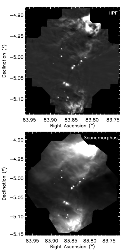
Figure 8: A comparison of 70 µm maps of Group 019 in OMC 2/3, generated with the high-pass filter technique (top) and the Scanamorphos technique (bottom). The high-pass filter technique preserves point sources while suppressing extended structure, and the Scanamorphos technique preserves extended structure.

Appendix C Photometry

Photometry is challenging in star-forming regions. It is necessary to distinguish spatially unresolved knots in the nebular emission from actual point sources and to estimate the local background contribution. The nebular emission is usually complex and contains gradients of emission at all spatial scales that violate the common assumption of constant or smoothly varying backgrounds. It is also difficult to disentangle contributions from multiples with separations similar to the angular resolution of the image. We resolved these issues with multiple approaches to map-making and photometry. The photometry catalog was created by selecting the best approach for each source.

C.1 Aperture Photometry

We used the HPF images for aperture photometry. With ATV (Barth, 2001), we manually determined the appropriate parameters for the process, and with PhotVis (Gutermuth et al., 2008), we automatically identified sources and performed the photometry. Both procedures are based on aper.pro from the IDL Astronomy User’s Library (Landsman, 1993). To avoid nebular contamination from the local environment, we used annuli that are small and adjacent to the source to estimate the background contribution. This step necessitated customized aperture corrections, since the background annuli include a significant fraction of a source’s PSF profile. We used a calibration image of the asteroid Vesta (PACS’s PSF standard; see Lutz 2015) to calculate aperture corrections.

We set the inner radius of the sky annulus to the aperture radius to ensure the sky annulus samples the spatially varying nebulosity near the source. At 70 µm, we used an aperture radius of 9.6″, with the sky annulus extending from 9.6″ to 19.2″. At 160 µm, we used an aperture radius of 12.8″, with the sky annulus extending from 12.8″ to 25.6″. The aperture corrections are 0.7331 and 0.6602 at 70 µm and 160 µm; the measured fluxes were divided by these factors to account for flux outside the aperture.

Aperture photometry has several benefits. It is a reliable and well-understood technique, and it is the technique used for PACS flux calibration (Balog et al., 2014). Further, the use of narrow apertures as described above reduces the effect of contamination and crowding for most sources. However, complex structure in the images may still result in large uncertainties in the aperture photometry of a significant fraction of the sources. The primary problem is flux contamination from a neighboring source or extended emission in either the aperture or the sky annulus. Since the annuli are narrow and few pixels are available for sky estimation, this region can be particularly affected by the presence of a strong source. Contamination has a larger effect on the 160 µm measurements, because there is more extended emission at that wavelength. For the strongly affected sources in crowded or confused fields, we used PSF-fitting photometry as discussed in the next subsection.

C.2 Point Spread Function Fitting Photometry

In PSF-fitting photometry, a known spatial profile for point sources is fit to the measured point-source profiles, and the source brightnesses are determined from the scaling needed to make the known and measured profiles agree (Stetson, 1987). The primary advantage of this technique is that it disentangles the spatial profile of the source from other point sources and emission from the local environment.

This technique requires the source PSF profiles to be well characterized. The PACS PSF is highly non-axisymmetric (Lutz, 2015), requiring an accurate model. Given that no entirely contamination-free sources are available in our HOPS fields, we used images of Vesta as a proxy for the PSF profiles of our sources. To remove any systematic photometry offsets between PSF-based photometry and aperture-based photometry, we repeated the PSF measurements on a subset of PACS flux standard stars. This comparison allowed us to calibrate measured PSF amplitudes with actual flux measurements.

We used the StarFinder package (Diolaiti et al., 2000) for fitting PSF profiles and measuring photometry of sources in the Scanamorphos-reduced images. If there were overlapping sources, we fit them simultaneously even if not all were explicit HOPS targets. The StarFinder source-finding algorithm suffers from the same challenges as other algorithms, in that many of the detected sources are partially resolved or unresolved compact structures in the nebular emission. On the other hand, the PhotVis source finder used for aperture photometry circumvents this problem by using the local confusion noise surrounding each source to set a threshold for detection. We therefore limited our PSF-fitted photometry to protostars for which aperture photometry was known to be unreliable.

C.3 Final Photometry and Uncertainties

Since the aperture photometry might be contaminated by the presence of other nearby sources and spatially extended nebular emission, we inspected the images of each HOPS protostar individually. This inspection identified contaminants such as other point sources within the aperture radius or strong nebular features that were likely to affect photometry. Once identified as contaminated, we considered both PSF-fitted and aperture photometry in the context of the overall SED for the source. Aperture photometry for contaminated sources was rejected in favor of PSF-fitted photometry.

Of the 373 unique HOPS targets observed by PACS, we detected 338 (91%) in at least one of the 70 µm and 160 µm bands. Of the 338 detections, 253 (75%) were detected in both bands, 84 (25%) were detected at only 70 µm, and one was detected at only 160 µm. Of the 337 detections at 70 µm, 276 were measured with aperture photomery, and 61 were measured with PSF-fitting photometry. Of the 254 detections at 160 µm, 150 were measured with aperture photomery, and 104 were measured with PSF-fitting photometry. The expanded role of PSF-fitting photometry at 160 µm reflects how the colder protostellar envelope dust probed at longer wavelengths is less distinct from the dense cloud structures in which the protostars are forming. It is also a consequence of the lower resolution of the 160 µm maps and, therefore, higher likelihood of source blending compared to the 70 µm maps.

Aperture photometry uncertainties are calculated using the root-mean-square (RMS) variation in the intensity values within the sky annulus, but with a floor of 5%. PSF-fitting photometry uncertainties are set to 10% of the measured flux. When a source was observed more than once, only the observation with the longest exposure time appears in Table 2. We averaged all individual measurements to obtain the final estimate of its flux, and the reported uncertainty is the RMS of the individual uncertainties.

References

- Ali et al. (2010) Ali, B., Tobin, J. J., Fischer, W. J., et al. 2010, A&A, 518, L119
- Balog et al. (2014) Balog, Z., Müller, T., Nielbock, M., et al. 2014, ExA, 37, 129
- Barth (2001) Barth, A. J. 2001, in ASP Conf. Ser. 238, Astronomical Data Analysis Software and Systems X, ed. F. R. Harnden, Jr., F. A. Primini, & H. E. Payne (San Francisco, CA: ASP), 385
- Brown et al. (1994) Brown, A. G. A., de Geus, E. J., & de Zeeuw, P. T. 1994, A&A, 289, 101
- Carpenter (2000) Carpenter, J. M. 2000, AJ, 120, 3139
- Diolaiti et al. (2000) Diolaiti, E., Bendinelli, O., Bonaccini, D., et al. 2000, Proc. SPIE, 4007, 879
- Dunham et al. (2013) Dunham, M. M., Arce, H. G., Allen, L. E., et al. 2013, AJ, 145, 94
- Dunham et al. (2014) Dunham, M. M., Stutz, A. M., Allen, L. E., et al. 2014, in Protostars and Planets VI, ed. H. Beuther, R. Klessen, K. Dullemond, & T. Henning (Tucson, AZ: Univ. Arizona Press), 195
- Fischer et al. (2010) Fischer, W. J., Megeath, S. T., Ali, B., et al. 2010, A&A, 518, L122
- Fischer et al. (2017) Fischer, W. J., Megeath, S. T., Furlan, E., et al. 2017, ApJ, 840, 69
- Fischer et al. (2012) Fischer, W. J., Megeath, S. T., Tobin, J. J., et al. 2012, ApJ, 756, 99
- Fischer et al. (2019) Fischer, W. J., Safron, E., & Megeath, S. T. 2019, ApJ, 872, 183
- Furlan et al. (2016) Furlan, E., Fischer, W. J., Ali, B., et al. 2016, ApJS, 224, 5
- Furlan et al. (2014) Furlan, E., Megeath, S. T., Osorio, M., et al. 2014, ApJ, 786, 26
- González-García et al. (2016) González-García, B., Manoj, P., Watson, D. M., et al. 2016, A&A, 596, A26
- González Lobos & Stutz (2019) González Lobos, V., & Stutz, A. M. 2019, MNRAS, 489, 4771
- Großschedl et al. (2018) Großschedl, J. E., Alves, J., Meingast, S., et al. 2018, A&A, 619, A106
- Gutermuth et al. (2008) Gutermuth, R. A., Myers, P. C., Megeath, S. T., et al. 2008, ApJ, 674, 336
- Hacar et al. (2020) Hacar, A., Hogerheijde, M. R., Harsono, D., et al. 2020, A&A, in press
- Karnath et al. (2020) Karnath, N., Megeath, S. T., Tobin, J. J., et al. 2020, ApJ, 890, 129
- Kounkel et al. (2018) Kounkel, M., Covey, K., Suárez, G., et al. 2018, AJ, 156, 84
- Kounkel et al. (2016) Kounkel, M., Megeath, S. T., Poteet, C. A., Fischer, W. J., & Hartmann, L. 2016, ApJ, 821, 52
- Kryukova et al. (2012) Kryukova, E., Megeath, S. T., Gutermuth, R. A., et al. 2012, AJ, 144, 31
- Kryukova et al. (2014) Kryukova, E., Megeath, S. T., Hora, J. L., et al. 2014, AJ, 148, 11
- Lada et al. (2009) Lada, C. J., Lombardi, M. & Alves, J. F. 2009, ApJ, 703, 52
- Landsman (1993) Landsman, W. B. 1993, in ASP Conf. Ser. 52, Astronomical Data Analysis Software and Systems II, ed. R. J. Hanisch, R. J. V. Brissenden, & J. Barnes (San Francisco, CA: ASP), 246
- Lutz (2015) Lutz, D. 2015, PACS Photometer Point Spread Function, Document PICC-ME-TN-033 (Madrid: HSC), http://herschel.esac.esa.int/twiki/pub/Public/PacsCalibrationWeb/bolopsf_22.pdf
- Manoj et al. (2016) Manoj, P., Green, J. D., Megeath, S. T., et al. 2016, ApJ, 831, 69
- Manoj et al. (2013) Manoj, P., Watson, D. M., Neufeld, D. A., et al. 2013, ApJ, 763, 83
- Megeath et al. (2012) Megeath, S. T., Gutermuth, R., Muzerolle, J., et al. 2012, AJ, 144, 192
- Megeath et al. (2016) Megeath, S. T., Gutermuth, R., Muzerolle, J., et al. 2016, AJ, 151, 5
- Osorio et al. (2017) Osorio, M., Díaz-Rodríguez, A. K., Anglada, G., et al. 2017, ApJ, 840, 36
- Ott (2010) Ott, S. 2010, in ASP Conf. Ser. 434, Astronomical Data Analysis Software and Systems XIX, ed. Y. Mizumoto, K.-I. Morita, & M. Ohishi (San Francisco, CA: ASP), 139
- Pilbratt et al. (2010) Pilbratt, G. L., Riedinger, J. R., Passvogel, T., et al. 2010, A&A, 518, L1
- Poglitsch et al. (2010) Poglitsch, A., Waelkens, C., Bauer, O. H. et al. 2010, A&A, 518, L2
- Pokhrel et al. (2020) Pokhrel, R., Gutermuth, R. A., Betti, S. K., et al. 2020, ApJ, 896, 60
- Popesso et al. (2012) Popesso, P., Magnelli, B., Buttiglione, S., et al. 2012, arXiv:1211.4257
- Rezaei Kh. et al. (2020) Rezaei Kh., S., Bailer-Jones, C. A. L., Soler, J. D., & Zari, E. 2020, arXiv:2007.01331
- Roussel (2013) Roussel, H. 2013, PASP, 125, 1126
- Sadavoy et al. (2014) Sadavoy, S. I., Di Francesco, J., André, P., et al. 2014, ApJ, 787, L18
- Safron et al. (2015) Safron, E. J., Fischer, W. J, Megeath, S. T., et al. 2015, ApJ, 800, L5
- Skrutskie et al. (2006) Skrutskie, M. F., Cutri, R. M., Stiening, R., et al. 2006, AJ, 131, 1163
- Stanke et al. (2010) Stanke, T., Stutz, A. M., Tobin, J. J., et al. 2010, A&A, 518, L94
- Stetson (1987) Stetson, P. B. 1987, PASP, 99, 191
- Stutz (2018) Stutz, A. M. 2018, MNRAS, 473, 4890
- Stutz & Gould (2016) Stutz, A. M., & Gould, A. 2016, A&A, 590, A2
- Stutz & Kainulainen (2015) Stutz, A. M., & Kainulainen, J. 2015, A&A, 577, L6
- Stutz et al. (2013) Stutz, A. M., Tobin, J. J., Stanke, T., et al. 2013, ApJ, 767, 36
- Tegmark (1997) Tegmark, M. 1997, ApJ, 480, L87
- Tobin et al. (2016) Tobin, J. J., Stutz, A. M., Manoj, P., et al. 2016, ApJ, 831, 36
- Tobin et al. (2015) Tobin, J. J., Stutz, A. M., Megeath, S. T., et al. 2015, ApJ, 798, 128
- Whitney et al. (2003) Whitney, B. A., Wood, K., Bjorkman, J. E., & Wolff, M. J. 2003, ApJ, 591, 1049
- Wilson et al. (1999) Wilson, T. L., Mauersberger, R., Gensheimer, P. D., Muders, D., & Bieging, J. H. 1999, ApJ, 525, 343
- Zucker et al. (2020) Zucker, C., Speagle, J. S., Schlafly, E. F., et al. 2020, A&A, 633, A51