Evolutionary Models for the Remnant of the Merger of Two Carbon-Oxygen Core White Dwarfs

Abstract

We construct evolutionary models of the remnant of the merger of two carbon-oxygen (CO) core white dwarfs (WDs). With total masses in the range $1-2\,\mathrm{\mathrm{M}_{\odot}}$, these remnants may either leave behind a single massive WD or undergo a merger-induced collapse to a neutron star (NS). On the way to their final fate, these objects generally experience a $\sim 10\,\mathrm{kyr}$ luminous giant phase, which may be extended if sufficient helium remains to set up a stable shell-burning configuration. The uncertain, but likely significant, mass loss rate during this phase influences the final remnant mass and fate (WD or NS). We find that the initial CO core composition of the WD is converted to oxygen-neon (ONe) in remnants with final masses $\gtrsim 1.05\,\mathrm{\mathrm{M}_{\odot}}$. This implies that the CO core / ONe core transition in single WDs formed via mergers occurs at a similar mass as in WDs descended from single stars, and thus that WD-WD mergers do not naturally provide a route to producing ultra-massive CO-core WDs. As the remnant contracts towards a compact configuration, it experiences a “bottleneck” that sets the characteristic total angular momentum that can be retained. This limit predicts single WDs formed from WD-WD mergers have rotational periods of $\approx 10-20\,\mathrm{min}$ on the WD cooling track. Similarly, it predicts remnants that collapse can form NSs with rotational periods $\sim 10\,\mathrm{ms}$.

1 Overview

The merger of two white dwarfs (WDs) can have a range of outcomes depending on the masses and compositions of the WDs (e.g., Webbink, 1984; Iben & Tutukov, 1985). The merger of a He WD with another He WD or low mass CO WD re-initiates stable He burning and the resulting merged object spends nuclear timescales $(\sim 10^{5}-10^{8}\,\mathrm{yr})$ as a hot subdwarf or R CrB star, before eventually going down the cooling track as a single WD (e.g., Schwab, 2018, 2019). In the case of mergers involving more massive WDs, the focus has primarily been on systems where the merger is likely to promptly lead to an explosive transient like a Type Ia supernova (e.g., Shen et al., 2018; Perets et al., 2019). Our current theoretical understanding does not definitively map the WD masses at merger to the set of possible final outcomes. However, it seems likely that there is at least some subset of WD-WD mergers with total mass $\gtrsim 1\,\mathrm{\mathrm{M}_{\odot}}$ that do not immediately destroy the system (i.e., the primary WD does not detonate).

In the non-destructive case, this leaves behind a $\approx~{}1-2\,\mathrm{\mathrm{M}_{\odot}}$ CO-dominated merger remnant. Broadly, the outcome is expected to be dependent on the remnant mass, with systems below the Chandrasekhar mass ($\mathrm{M}_{\rm Ch}$) producing massive single WDs and systems above $\mathrm{M}_{\rm Ch}$ undergoing a merger-induced collapse (MIC) to form a neutron star (NS; Nomoto & Iben, 1985; Saio & Nomoto, 1985). Schwab et al. (2016) demonstrated that this latter process may proceed through the formation of a low-mass iron core, evolving similarly to the exposed, low-mass metal cores found in the progenitors of ultra-stripped supernovae (e.g., Tauris et al., 2015).

Ongoing observational developments motivate understanding the signatures of WD-WD mergers in this mass range. Recent work demonstrates that there is class of massive ($\approx 0.8-1.3\,\mathrm{\mathrm{M}_{\odot}}$) DQ WDs with distinguishing chemical and kinematic properties (Dunlap & Clemens, 2015; Coutu et al., 2019; Koester & Kepler, 2019; Cheng et al., 2019). These objects have been suggested to be WD-WD merger remnants, but seem too He-poor and too massive to be the descendants of the R CrB stars. Further kinematic analysis of Gaia data suggests $\approx 20\%$ of all massive WDs may be merger products (Cheng et al., 2020). Other peculiar individual objects have emerged. Hollands et al. (2020) report a massive WD ($\approx 1.15\,\mathrm{\mathrm{M}_{\odot}}$) with an unusual carbon-hydrogen atmosphere and fast kinematics, potential signatures of a merger. Gvaramadze et al. (2019) report the detection of a hot, luminous object in a H-and-He-free nebula that roughly resembles the predictions of Schwab et al. (2016) for the properties of a double CO WD merger remnant $\sim 10$ kyr post-merger.

A theoretical understanding of the evolution of WD-WD merger remnants begins with knowledge of the conditions that develop in the immediate aftermath of the dynamically-unstable mass transfer in that can occur in these double-degenerate binaries. Modern insight came via smoothed-particle hydrodynamics (SPH) simulations by Benz et al. (1990) and has been refined over the subsequent decades. Beginning from this post-merger configuration, one must then follow the remnant into its longer-duration phases. In an early milestone, Segretain et al. (1997) created hydrostatic models that resembled merged configurations and used them to suggest the likely importance of the loss of mass and angular momentum from the remnant. In a pioneering work, Yoon et al. (2007) modeled WD-WD merger remnants by performing stellar evolution calculations beginning from initial conditions based on the results of WD-WD merger simulations. Much subsequent work, including this paper, follows in that vein.

Here, we construct simple evolutionary models of WD-WD merger remnants with (initially) CO cores and total masses $\gtrsim 1\,\mathrm{\mathrm{M}_{\odot}}$. Our goal is to investigate their final fates and describe the effects of key physical processes on the post-merger evolution. Section 2 describes how we construct our initial conditions and Section 3 describes the baseline post-merger evolution. Sections 4, 5, and 6 discuss the additional effects of mass loss, nuclear burning, and rotation, respectively. In Section 7 we summarize and conclude.

2 Models

We construct stellar evolution models of the merger remnants using MESA r12778 (Paxton et al., 2011, 2013, 2015, 2018, 2019). The initial models are guided by the post-dynamical-phase structures from Dan et al. (2014), but we do not attempt to directly map these results into MESA. Instead, we create a set of parameterized initial MESA models that reflect the key features of the remnant structure and schematically include the effects of the viscous phase (Shen et al., 2012; Schwab et al., 2012). We first describe the procedure that we use to construct non-rotating, pure carbon-oxygen models and then later describe how we extend these models to explore the effects of rotation and the presence of helium.

2.1 Initial Conditions

Dan et al. (2014) performed a large set of WD merger simulations that span the space of mass/composition for each of the primary and secondary WD. Thermodynamic and rotational profiles of their models were previously available online. Their HeCO WDs have masses 0.50, 0.55, and 0.60 $\mathrm{M}_{\odot}$ and have pure CO cores ($X_{\mathrm{C}}=X_{\mathrm{O}}=0.5$) overlaid by a $0.1\,\mathrm{\mathrm{M}_{\odot}}$ pure-He mantle. Their CO WDs have masses $0.65-1.05$ $\mathrm{M}_{\odot}$ and are pure carbon-oxygen ($X_{\mathrm{C}}=0.4,X_{\mathrm{O}}=0.6$) throughout. In this work, our default assumption for the composition of the models is pure CO ($X_{\mathrm{C}}=0.4,X_{\mathrm{O}}=0.6$), but Section 5 discusses the effects of the presence of He.

The Dan et al. (2014) calculations follow the merger through its dynamical phase—covering three orbital periods after the donor is disrupted—and result in the formation of a roughly axisymmetric remnant. Shen et al. (2012) emphasize the importance of a subsequent viscous phase of evolution, lasting for $\sim 10^{4}-10^{8}\,\mathrm{s}$, during which angular momentum (AM) transport due to magnetohydrodynamic (MHD) processes brings the remnant toward solid-body rotation long before significant cooling can occur. The effects of this phase are important to include, but are challenging to follow with numerical simulations (e.g., Schwab et al., 2012; Ji et al., 2013).

The information made publicly available by Dan et al. (2014) are 1D profiles (slices and equipotential averages) of their simulations. These are not sufficient to directly initialize multi-D hydrodynamic simulations of the viscous phase like those performed in Schwab et al. (2012) and MESA does not have appropriate capabilities for approximately following the viscous phase in 1D. As such, we elect instead to schematically include the effects of the viscous phase (described in more detail below). Future work directly modeling the viscous phase can eliminate some of the uncertainties introduced by our schematic approach.

Dan et al. (2014) divide the remnant into 4 components: the core, hot envelope, disk, and tidal tail. We use their provided fitting formulae (which are functions of total mass and mass ratio) to set the masses of each of these components. We identify each of our models primarily by its mass ratio and total mass (i.e., “the $q=2/3$, $M_{\rm tot}=1.5\,\mathrm{M}_{\odot}$ model”).

The tidal tail accounts for at most a few percent of the total mass and we therefore ignore it. We neglect any mass unbound from the system (so that the initial remnant mass remains the same as the total mass of the merging WDs) and do not attempt to include the effect of tidal tail material that may remain bound and fall back. However, we do note that this cool tidal tail material is a potential reservoir of unburned H or He. This material could then be incorporated into the outer layers of the remnant as the remnant expands and/or the tidal material returns from apocenter. This might provide an avenue for creating thin H/He layers on merger remnant WDs.

The core is the inner portion of the primary WD. Our initial model has an isothermal core of mass $M_{\rm core}$ with temperature $T_{\rm core}$. The precise temperature of this material is generally unimportant, so long as it is degenerate. We typically assume $T_{\rm core}\approx 10^{8}\,\mathrm{K}$.

The hot envelope is material that was shock heated in the merger. This is exterior to the core and includes the initial outer layers of the primary. Because the viscous evolution will also transform the disk material into a hot envelope, we instead refer to this region of the model as the “peak”, since it contains the temperature peak. This region has a mass $M_{\rm peak}$ with a maximum temperature $T_{\rm peak}$. We assign this region an entropy profile that linearly increases with mass coordinate and connects the low-entropy core and the high-entropy disk.

Figure 1 shows the $T_{\rm max}$ values reported in Dan et al. (2014) as a function of the total mass of the merging WDs. The value of $T_{\rm max}$ is the maximum over the simulation and so typically reflects a localized hot region. The squares in Figure 1 show the maximum temperature extracted from the equipotential-averaged, 1D profiles of the Dan et al. (2014) models. These temperature values are systematically lower than $T_{\rm max}$ and would more accurately reflect the temperatures implied by a direct mapping of the post-dynamical phase structure into (1D) MESA. However, in the viscous calculations of Schwab et al. (2012), the peak temperature increases relative to its value at the end of the dynamical phase. This is primarily due to adiabatic compression from material above as the rotational support of the disk material is removed (though in some cases additional entropy can be injected due to nuclear burning). Therefore, by using the higher $T_{\rm max}$, we are assuming that these two differences approximately offset. As a check of this crude assumption, the Xs in Figure 1 mark the final maximum temperature from the end of two viscous-phase calculations. On the basis of this limited check, there is no indication that this choice is dramatically incorrect.

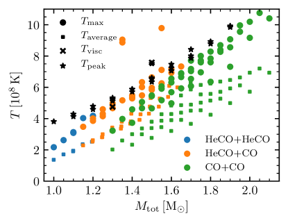
Figure 1: Maximum temperature versus total mass of the merging WDs from Dan et al. (2014). Larger circles show the maximum SPH particle temperature while smaller squares show the maximum value from equipotential-averaged profiles. Colors indicate the compositions of the merging WDs. The Xs indicate the maximum temperature of two models after simulations of the viscous evolution (see text). The stars mark the peak temperatures of the initial models used in this work.

The disk material is primarily the tidally disrupted secondary and is initially rotationally supported. Viscous dissipation subsequently heats this material as its angular momentum is transported outward. Schwab et al. (2012) found that this region became convectively unstable and thus evolved towards an entropy profile that is roughly spatially constant. Therefore, we assign this material such a state. Because we do not directly simulate the viscous phase, we do not know the precise entropy to target, so instead we select a total-mass-dependent entropy that gives us the desired trend in $T_{\rm peak}$. The state of the outer layers is the most artificial aspect of our treatment. This limits the predictive power of our models in their earliest phases. However, after the first few thermal times of this envelope elapse, we expect its state to be reset by the luminosity from the hot material below.

In practice, our prescription is as follows. We begin with a high entropy carbon-oxygen MESA model of the desired mass and relax its temperature/entropy following a procedure similar to that described in Appendix A of Schwab et al. (2016). Our target profile is: for $0\leq M_{r}\leq M_{\rm core}$,

$$T(M_{r})=T_{\rm core}~{};$$

for $M_{\rm core}\leq M_{r}\leq M_{\rm core}+M_{\rm env}$,

$$s(M_{r})=s_{\rm core}+[s_{\rm env}-s(M_{\rm core})]\frac{M_{r}-M_{\rm core}}{M_{\rm peak}}~{};$$

and for $M_{\rm core}+M_{\rm env}<M_{r}\leq M_{\rm tot}$,

$$s(M_{r})=s_{\rm env}~{}.$$

We adopt $T_{\rm core}=10^{8}\,\mathrm{K}$ and the ad hoc relationship $\log(s_{\rm env}/\rm erg\,g^{-1}\,K^{-1})=8.7+0.3\left(M_{\rm tot}/\mathrm{M}_{\odot}-1.5\right)$ in order to achieve the desired $M_{\rm tot}$ vs. $T_{\rm peak}$ relationship shown in Figure 1. Given this somewhat arbitrary form, in Section 3 we show models at a fixed mass with varying values of $s_{\rm env}$ to illustrate that the evolutionary trajectory is not sensitive to this choice.

In Figure 2, we demonstrate that this approach provides a reasonable starting condition. We compare with the post-viscous-phase model of a $0.6+0.9\,\mathrm{\mathrm{M}_{\odot}}$ CO+CO WD merger from Schwab et al. (2012) as the detailed entropy profile of this model provided the initial condition for the fiducial model in Schwab et al. (2016). The schematic model reproduces the key features, namely a hot envelope overlaying a cold core. The dotted lines show the 1D equipotential-averaged, post-dynamical-phase profiles from Dan et al. (2014). The differences from the post-viscous-phase model above the core (at $M_{r}\gtrsim 0.65\,\mathrm{\mathrm{M}_{\odot}}$) illustrate the increase in the peak temperature and the envelope entropy that occur during the viscous phase. As it was designed to do, the schematic approach provides an initial condition that is a closer match to the peak temperature and envelope entropy of the more detailed post-viscous-phase model than a model beginning directly from a Dan et al. (2014) profile.

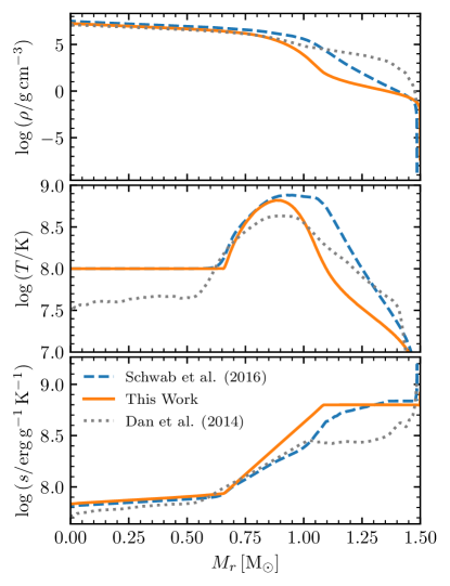
Figure 2: Thermodynamic profiles of the parameterized initial model used in this work (solid lines). For comparison, we show (dashed lines) the equivalent initial model from Schwab et al. (2016), which was based on a higher resolution SPH simulation from Dan et al. (2011) and a simulation of the viscous phase from Schwab et al. (2012). We also show (dotted lines) the 1D equipotential-averaged, post-dynamical-phase profiles from Dan et al. (2014).

While lacking some of the consistency that would come from a more elaborate viscous-phase simulation of the merger, the simple parameterized nature of these initial conditions allows us to easily generate families of models that vary the total mass and mass ratio. Figure 3 illustrates how the temperature profiles vary in two such families.

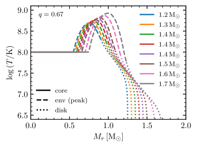
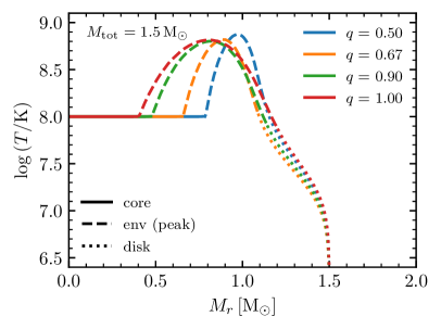
Figure 3: Temperature profiles of families of parameterized initial models. The top (bottom) panel shows a sequence of models at fixed (varying) mass ratio and varying (fixed) total mass. The line style indicates the different components following the Dan et al. (2014) subdivision.

2.2 Input Physics

We use the OPAL radiative opacities for C- and O-rich mixtures (Iglesias & Rogers, 1993, 1996), referred to as “Type 2” tables in MESA, with a base metallicity $Z=0.02$. The stellar models evolve to temperatures below the lower boundary of the OPAL tabulations ($\log(T/\rm K)<3.75$), so we supplement this with the low-temperature table generated in Schwab et al. (2016)—see their Appendix B—that smoothly extends the opacities to lower temperatures.

The MESA equation of state (EOS) compilation does not include any component EOS that covers CO mixtures and includes ionization of these metals. Therefore, in the regions [$\log(T/\rm K)\lesssim 7.7$ and $\log(\rho/\mathrm{g\,cm^{-3}})\lesssim 3.5$] that would normally be covered by the OPAL and/or PTEH EOSes when $Z<1$, we instead use the HELM EOS (Timmes & Swesty, 2000). HELM includes an ideal gas of ions, a Fermi-Dirac electron gas, and radiation. It parameterizes composition by the mean ion weight and charge. HELM is a physically suitable choice for when material is fully ionized and is also the EOS used in the merger simulations of Dan et al. (2011, 2014). The default behavior in MESA is to crudely mock up the effects of ionization by blending between versions of HELM including the contribution of electrons over the temperature range $\log(T/\rm K)=4.5-5.0$. In MESA r6596, as used in Schwab et al. (2016), this blend was hard coded in. In MESA r12778, this is user-configurable, and in this work, we deactivate this blend and so use an EOS assuming full ionization throughout. We use the 21 isotope, $\alpha$-chain nuclear network approx21.net.

As the remnant expands towards a giant structure, it develops radiation-pressure-dominated envelope that is locally super-Eddington. Convection, as modeled by mixing length theory (MLT), becomes inefficient and a steep entropy gradient develops at the base of the convective region. Tracking this narrow region is numerically demanding and often severely limits the timestep. To circumvent this, we apply the ad hoc “MLT++” prescription discussed in Paxton et al. (2013). This procedure essentially assumes a third (unspecified) pathway for energy transport, allowing the temperature gradient to be closer to adiabatic and the entropy gradient less steep.

Taken together, the limited opacities, lack of appropriate EOS, and and use of MLT++ mean that the outer layers of our stellar models are poorly modeled. The luminosity is typically set by the energy transport in the deeper, better-modeled layers, but the radii/effective temperatures of our models are best understood as qualitative predictions.

2.3 Stopping Conditions

We evolve the models until they either begin to go down the WD cooling track (stopping when $L<100\,\mathrm{\mathrm{L}_{\odot}})$ or experience off-center Ne ignition. For those models that experience Ne ignition, we are unable to follow the models further due to the computational expense of resolving the thin neon-oxygen-burning flames that develop. (The one such calculation reported in Schwab et al. (2016) took months to run.) However, because the Ne/O-burning flames are relatively fast $(\sim 10\,\rm cm\,s^{-1}$) and subsequent Si-burning flames even faster $(\sim 10^{3}\,\rm cm\,s^{-1}$), the timescales for these burning stages are $\sim 10\,\mathrm{yr}$ and $\sim 0.1\,\mathrm{yr}$ respectively (Timmes et al., 1994; Woosley & Heger, 2015). As such, while the core continues to evolve in response to these burning processes, we expect that the outer layers are approximately frozen at this time. Therefore, while we do not model it, we expect the remnants that experience Ne ignition and are above $\mathrm{M}_{\rm Ch}$ to undergo a MIC to form a NS via the formation of a low mass Fe core as outlined by Schwab et al. (2016). Those few remnants with masses sufficiently high to ignite Ne but that remain below $\mathrm{M}_{\rm Ch}$ may instead leave behind massive single WDs with Si-group or Fe-group core compositions.

2.4 Comparison with Schwab et al. (2016)

To compare the MESA setup used in this work with that in Schwab et al. (2016), we evolved the same fiducial initial model “M15”. Figure 4 shows the model track in the HR diagram from shortly after the merger until carbon burning reaches the center. The two M15 model tracks agree closely, though the time evolution is slightly different with the current setup, resulting in a model that spends less time in the reddest part of the HR diagram but moves to the blue more slowly. The analogous parameterized model shows more substantial differences, though these simply reflect its different initial structure.

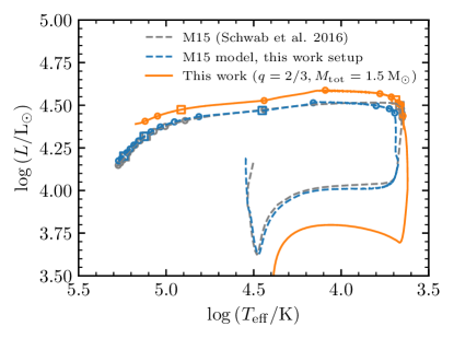
Figure 4: Comparison of the evolution of 0.6 $\mathrm{M}_{\odot}$ + 0.9 $\mathrm{M}_{\odot}$ merger models in the HR diagram. These models stop when carbon burning reaches the center of the remnant. Time moves counterclockwise along the tracks with small circles each kyr and larger squares every 5 kyr. The two dashed lines illustrate the small differences between model M15 from Schwab et al. (2016) and the result of this same initial model evolved using the MESA version and options adopted in this work. The solid line shows the result of the parameterized initial model adopted in this work, illustrating the differences in evolution due to the initial model differences shown in Figure 2.

3 Post Merger Remnants

To illustrate how the evolution depends on the properties of the merging binary, we generate families of initial models following the scheme described in Section 2.1. We focus on masses $M_{\rm tot}\approx 1-2\,\mathrm{\mathrm{M}_{\odot}}$ with mass ratios such that neither of the component WDs would likely be He WDs $(<0.5\,\mathrm{M}_{\odot})$ or ONe WDs $(>1.05\,\mathrm{M}_{\odot})$.

Figure 5 shows the evolution of some of these models in the HR diagram. The left panel shows a sequence at fixed mass $(M_{\rm tot}=1.5\,\mathrm{M}_{\odot})$ and varying mass ratio. All these models ignite carbon burning and terminate at Ne ignition. The HR evolution is similar and the duration of the evolution (indicated in legend) is also within $50\%$. Given the level to which we trust our input physics and the details of the initial models, we regard these tracks as effectively identical. These models do not predict a significant dependence on the mass ratio, where the main mass-ratio-dependent property is the initial location and width of the temperature peak region.

The right panel shows a sequence of models at fixed mass ratio $(q=0.9)$ and varying total mass. All models experience carbon ignition. The 1.1 $\mathrm{M}_{\odot}$ model becomes a ONe WD. The 1.3 $\mathrm{M}_{\odot}$ model experiences numerical problems after the C flame reaches the center. This appears to be associated with a high luminosity during the subsequent KH contraction phase (around its bluest extent). If this model were allowed to launch a wind in response, we expect that it would shed its outer layers (the source of the numerical issues) and become a massive ONe WD. The 1.5, 1.7, and 1.9 $\mathrm{M}_{\odot}$ models all reach Ne ignition. The models evolve more rapidly with increasing mass (18, 13, and 10 kyr respectively), with this most massive model reaching Ne ignition while it still has a relatively extended envelope $(R\approx 30\,\mathrm{R}_{\odot})$.

The luminosity roughly scales with the mass, being near-Eddington. The small dynamic range in expected remnant masses (at most a factor of 2) makes this likely to be challenging as an observational diagnostic, but our models do generically predict that more massive remnants are more luminous.

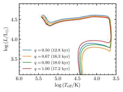
Figure 5: Model evolution in the HR diagram. Models stop when they undergo off-center Ne ignition or start to go down the WD cooling track. The left panel shows a sequence at fixed total mass $(M_{\rm tot}=1.5\,\mathrm{M}_{\odot})$ and the legend indicates the duration of the plotted track. The right panel shows a sequence of models at fixed mass ratio $(q=0.9)$. The green line is the same in the two plots. The total mass of the remnant is the most important parameter controlling its evolution.

The value of the parameter $s_{\rm env}$ in our models was set in an ad hoc way. In Figure 1, the peak temperatures in our remnant models with masses $\lesssim 1.2\,\mathrm{\mathrm{M}_{\odot}}$ are somewhat higher than those suggested by the merger calculations. Raising the envelope entropy will lower the peak temperature. Since the temperatures are already well below the $\sim 10^{9}\,\mathrm{K}$ associated with carbon burning, the initial nuclear energy release will be negligible and so we would not expect our results to be sensitive to modest variations in $T_{\rm peak}$. Figure 6 illustrates that varying $s_{\rm env}$ has only a minor effect on the evolution. The higher entropy models are puffier and so begin as giants on the HR diagram. Given the higher entropy, it also takes longer for the envelopes to cool and contract. The legend indicates the length of time between the start of the calculation and the initiation of carbon burning (marked by the dot).

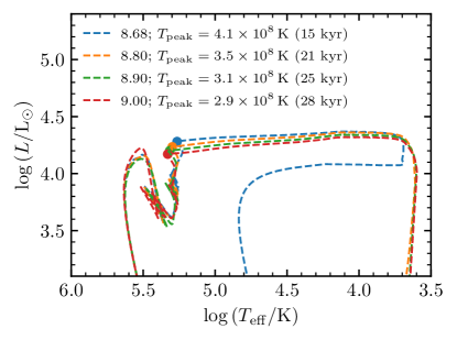
Figure 6: Comparison of evolution in the HR diagram for the $q=0.9$, $M_{\rm tot}=1.1\,\mathrm{M}_{\odot}$ model with varying values of the initial envelope entropy. The first number in each legend entry indicates the value $\log(s_{\rm env}/\rm erg\,g^{-1}\,K^{-1})$. This is followed by the initial peak temperature and the time from the start of the calculation until carbon is ignited (which is indicated by the solid dot). The overall evolution is not strongly influenced by this aspect of the initial condition.

4 Effects of Mass Loss

The thermal energy deposited as a result of the merger causes the remnant to inflate to giant radii ($\gtrsim 100\,\mathrm{\mathrm{R}_{\odot}}$). Given the CO-dominated composition of the envelope, it seems likely that these objects will drive dusty winds. The mass loss of such objects is not observationally well-constrained and we do not have a reliable way of theoretically estimating these mass loss rates. While the mass loss rate will be important for setting the observed properties of the remnant, the overall evolution—in particular the extent to which the object experiences C-burning and Ne-burning (and beyond)—is also influenced by the total amount of mass lost.

We explore the effect of mass loss using an ad hoc wind prescription. Given that the time spent as a giant is $\sim 10$ kyr, only mass loss rates $\gtrsim 10^{-5}\,\mathrm{M}_{\odot}\,\mathrm{yr^{-1}}$ can have a significant evolutionary effect by changing the total mass. We assume that the object will shed a fraction of its mass $f$ on a timescale $\frac{GM^{2}}{RL}$, evaluated at the surface. This implies a mass loss rate

$$\begin{split}\dot{M}=10^{-5}\,\mathrm{M}_{\odot}\,{\rm yr}^{-1}&\left(\frac{f}{10^{-4}}\right)\left(\frac{R}{100\,\mathrm{R}_{\odot}}\right)\\ \times&\left(\frac{L}{3\times 10^{4}\,\mathrm{L}_{\odot}}\right)\left(\frac{M}{\mathrm{M}_{\odot}}\right)^{-1},\end{split}$$ (1)

where our fiducial value of $f$ is selected to give $\dot{M}=10^{-5}\,\mathrm{M}_{\odot}\,\mathrm{yr^{-1}}$. Compared to an even simpler form like a constant, Equation (1) has the advantage that the mass loss rate is smaller when the object is compact and larger when the object is a luminous giant. When discussing models using this prescription, we will indicate the value of $f$ using the shorthand $f_{-4}\equiv f/10^{-4}$. This prescription is equivalent to the Reimers (1975) mass loss prescription for red giants with the scaling factor $\eta_{\rm R}\approx 10f_{-4}$. So $f_{-4}=1$ represents a larger mass loss rate than one would get assuming a typical value for normal red giants of $\eta_{\rm R}\approx 0.5$. The Bloecker (1995) mass loss prescription for asymptotic giant branch stars depends more steeply on $L$ and $M$, such that with $L\approx 3\times 10^{4}\,\mathrm{\mathrm{L}_{\odot}}$, $M\approx 1.5\,\mathrm{\mathrm{M}_{\odot}}$, and a typical scaling factor of $\eta_{\rm B}\approx 0.05$, it yields a factor of $\approx 250$ enhancement over the Reimers prescription. So a value $f_{-4}=1$ represents a lower mass loss rate than if we were to simply assume a Blöcker prescription.

Figure 7 shows the HR diagram evolution of the $q=2/3$, $M_{\rm tot}=1.5\,\mathrm{M}_{\odot}$ model with different scaling factors. The initial thermal adjustment phase is rapid, and so the differences only appear as the remnant reaches its longer-lived luminous giant phase and then begins to evolve to the blue. The model with the highest mass loss rate ($f_{-4}=10$) goes down the cooling track as a $\approx 1.2\,\mathrm{\mathrm{M}_{\odot}}$ ONe WD. The model with a somewhat lower rate ($f_{-4}=3$) shrinks to $\approx 1.3\,\mathrm{\mathrm{M}_{\odot}}$ and undergoes a similar excursion as the initially $1.3\,\mathrm{\mathrm{M}_{\odot}}$ model shown in Figure 5 before halting with the same numerical problems. If the evolution continued and the NeO-burning successfully reached the center, this might leave a WD with a Si-group core composition. The other three models with lower mass loss rates all remain $>1.35\,\mathrm{\mathrm{M}_{\odot}}$, experience off-center Ne ignition, and would likely go on to form low mass Fe cores and subsequently collapse to NSs. This illustrates how the amount of mass shed as a giant qualitatively alters the evolution and that the mass as the object leaves the giant phase controls the extent to which it undergoes advanced burning stages and the type of object it leaves behind.

We also ran a set of models with constant mass loss rates during the giant phase. Tracks with constant mass loss rates comparable to the values realized in the right panel of Figure 7 gave qualitative agreement in terms of the HR tracks and final outcomes. This shows that the evolution is not sensitive to the details of the mass loss prescription. We expect that prescriptions that give similar total mass loss over the giant phase will result in similar evolution.

All of the material lost during these phases has the initial composition of the WD. The carbon burning is ignited relatively deep in the remnant (around the temperature peak) and its neutrino-cooled convection zone does not extend to near the surface. Later, carbon flashes process material further out, and eventually only a CO surface layer of mass $\sim 10^{-2}\,\mathrm{M}_{\odot}$ remains. For representative Kippenhahn diagrams see Figures 2 and 5 in Schwab et al. (2016).

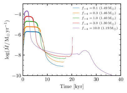
Figure 7: Comparison of the $q=2/3$, $M_{\rm tot}=1.5\,\mathrm{M}_{\odot}$ model with varying mass loss rates using the prescription given by Equation (1). The left panel shows the evolution in the HR diagram. The right panel shows the mass loss rate as a function of time. Most of the mass is lost in the vicinity of the luminous/cool corner of the evolutionary tracks; the thick portion of the matching lines in each panel indicate corresponding time intervals. The legend parenthetically indicates the mass at the end of the calculation.

5 Effects of Nuclear Burning

5.1 Helium burning

The presence of He surface layers on the CO WDs allows for the possibility of surface detonations and hence also double detonation scenarios for thermonuclear supernovae (e.g., Dan et al., 2015). Our approach is not suitable for cases where significant nuclear energy is released on the dynamical or viscous timescales. Rather, we consider the effects of nuclear energy release on the $\sim$ kyr evolutionary timescale of the remnants.

In Dan et al. (2014), their HeCO WDs have masses 0.50, 0.55, and 0.60 $\mathrm{M}_{\odot}$ and have pure CO cores overlaid by a $0.1\,\mathrm{\mathrm{M}_{\odot}}$ He mantle. This is a typical amount of He found on lower mass CO WDs in stellar evolution calculations (e.g., Zenati et al., 2019). Thus for mergers involving at least one lower mass CO WD ($\approx 0.5-0.7\,\mathrm{M}_{\odot}$), initially $\approx 10\%$ of the remnant mass may be He.

When the lower mass WD is tidally disrupted, its composition is mixed as it forms the disk/envelope. The outer layers of the primary WD are also mixed via the dredge-up action of the merger (Staff et al., 2018). The chemical profiles from the Dan et al. (2014) models are generally well-mixed, such that the He distribution can be reasonably approximated as a constant value of $X_{\rm He}$ in the disk/envelope component. (The He mass fraction is higher in the outermost layers reflecting material stripped early in the merger and now at larger radii, including the tidal tail.)

The presence of a significant amount of He suggests that the object will set up a steady He burning shell. This is similar to what happens in the formation of R CrB stars formed via He+CO WD mergers, with the main difference being that the burning shell is processing an envelope that is majority CO with a $\approx 10\%$ He mass fraction, as opposed to the R CrB envelopes which are mostly He with percent-level C abundances (e.g., Asplund et al., 2000). Given that CO core WDs are O-dominated, one other conspicuous difference may be a C/O number ratio $<1$, suggesting an O-rich surface chemistry in the cool outer layers.

This steady shell burning will extend the time the object spends in the giant phase. The specific energy associated with He burning is $Q_{\rm He}\approx 7\times 10^{17}\,\mathrm{erg\,g^{-1}}$. Given core masses $\gtrsim 0.6\,\mathrm{\mathrm{M}_{\odot}}$, the shell burning luminosity is expected to be a significant fraction of the Eddington luminosity (e.g., Jeffery, 1988; Saio, 1988). Thus, assuming all the He burns, the associated timescale is

$$t_{\rm giant}\sim 40\,\mathrm{kyr}\left(\frac{L}{3\times 10^{4}\,\mathrm{\mathrm{L}_{\odot}}}\right)\left(\frac{M_{\rm He}}{0.1\,\mathrm{\mathrm{M}_{\odot}}}\right)~{}.$$ (2)

That is similar to the lifetime of an R CrB star, reflecting the similar luminosities and amount of He. As discussed by Schwab (2019) in the R CrB context, if the mass loss rate becomes comparable to the rate at which mass is processed through the He burning shell, then the lifetime is limited by the removal of the reservoir of He in the envelope.

To illustrate the difference in evolution, we set $X_{\rm He}=0.1$ in the outer layers of the $q=0.90$, $M_{\rm tot}=1.1\,\mathrm{M}_{\odot}$ model. This adds a total mass of 0.04 $\mathrm{M}_{\odot}$ of He. This initial model is indicated as “CO + He”, while the model without He is indicated as “CO”. Figure 8 compares the evolutionary tracks in the HR diagram. The reference (both panels, solid, grey line) is the pure CO model without mass loss. In the run without mass loss (left panel, solid, blue line), the model with He spends approximately 10 times longer than the “CO” model (40 kyr vs. 4 kyr) in the giant phase. The increased luminosity and longer giant phase suggest that the presence of He will make mass loss an even more important effect. In a run of the “CO + He” model with mass loss (left panel, dotted, orange line), the object spends only $\approx 15$ kyr as a giant and does not reach such extreme luminosities.

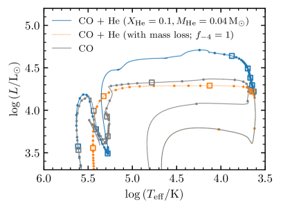
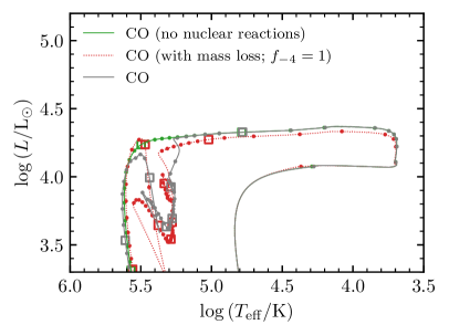
Figure 8: Evolution in the HR diagram of a $q=0.90$, $M_{\rm tot}=1.1\,\mathrm{M}_{\odot}$ remnant. Initial model “CO” has the default pure carbon-oxygen composition. Initial model “CO + He” has the indicated amount of He uniformly distributed in the disk/envelope material. Solid lines show models without mass loss; dotted lines show models that include mass loss. A small dot appears along the track each kyr and a large square each 10 kyr. The left panel illustrates that the presence of He and the energy release from He burning extends the time spent as a giant by $\sim 10$ kyr. The right panel illustrates the limited influence of carbon burning during the giant phase. (See text for more discussion.)

5.2 Carbon burning

Figure 8 we show the case (right panel, solid, green line) of the “CO” model in which nuclear reactions are not included. The evolution on the right of the HR diagram is the same, reflecting that this phase radiates the thermal energy deposited in the merger, not nuclear energy from carbon burning. On the left of the HR diagram, the case without nuclear reactions simply goes down the cooling track as a massive CO WD. This track notably lacks the drop in $L$ around $\log(T_{\rm eff}/\rm K)=5.3$ that is present in other models. This feature is associated with carbon ignition (see marked point in Figure 6), the propagation of the carbon burning to the center, and subsequent of carbon flashes in the outer layers. Therefore, tracks with this feature that also go down the cooling track leave behind an ONe WD.

Note that in the case with He burning and mass loss (left panel, dotted, orange line), this feature is absent. The mass loss led to less compression around the location of the temperature peak and a long-lived carbon-burning front did not form. The remnant in this case is a $0.91\,\mathrm{\mathrm{M}_{\odot}}$ CO WD (with $3\times 10^{-4}\,\mathrm{\mathrm{M}_{\odot}}$ of He). By contrast, the “CO” model evolved with the same mass loss prescription (right panel, dotted, red line), but lacking the He-burning-associated mass loss, reaches the cooling track as an $1.06\,\mathrm{\mathrm{M}_{\odot}}$ ONe WD.

This illustrates that variations in the mass loss rate affect whether particular advanced nuclear burning stages occur. If we vary the mass loss rate scaling factor for the $q=0.9$, $M_{\rm tot}=1.1\,\mathrm{M}_{\odot}$ model, the $f_{-4}=10$ case leaves behind a $1.02\,\mathrm{\mathrm{M}_{\odot}}$ CO WD, whereas the $f_{-4}=3$ case leaves a $1.04\,\mathrm{\mathrm{M}_{\odot}}$ ONe WD. Our models change whether or not they experience C-ignition within the (post-giant-phase) mass range $\approx 1.0-1.1\,\mathrm{\mathrm{M}_{\odot}}$. Figure 7 shows the similar change for Ne-ignition occurring within a mass range $\approx 1.3-1.4\,\mathrm{\mathrm{M}_{\odot}}$. Figure 9 illustrates how the outcome varies with the initial total mass at merger and the final remnant mass. These transition masses are not dissimilar from the typical characteristic masses in single star evolution.

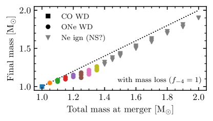
Figure 9: Final masses (and remnant type) for a set of models with varying total mass and mass ratio. The dotted line marks conservative evolution (final mass equals initial mass). Since our models stop at Ne ignition, we cannot definitely say these form NSs, but that outcome seems inevitable for anything that remains super-Chandrasekhar (i.e., all but the lowest mass set of grey triangles, which might instead leave an Si- or Fe-group core WD).

5.2.1 Implications for WD core compositions

In single stars, the transition from CO WDs to ONe WDs is marked by the occurrence of off-center carbon ignition in the degenerate, neutrino-cooled CO core. The characteristic core mass for this process to occur was calculated by Murai et al. (1968), who performed calculations of contracting CO cores and found a minimum mass for carbon ignition of 1.06 $\mathrm{M}_{\odot}$. This early estimate matches the maximum mass of $\approx 1.06\,\mathrm{\mathrm{M}_{\odot}}$ found in modern calculations of single star evolution (e.g., Doherty et al., 2015).

The thermal structure of the merger remnants is not identical to the CO cores in single stars, but is similar, with an off-center temperature peak above a degenerate core. Carbon burning is not directly ignited by the merger in the lower mass merger remnants relevant for understanding the CO / ONe transition. Rather, the compressional heating at the base of the cooling envelope leads to carbon ignition. This compression-induced ignition has long been understood from work treating the WD-WD merger as the Eddington-limited accretion of the secondary onto the primary (Nomoto & Iben, 1985; Saio & Nomoto, 1985). Within this framework, Kawai et al. (1987) found ignition in CO WDs to occur at a mass 1.07 $\mathrm{M}_{\odot}$. While we argue against the details of the accretion picture, the compression at the base of a cooling envelope radiating at the Eddington luminosity is similar to the compression at the base of the accreted layer in an object accreting at the Eddington rate (Shen et al., 2012). Consistent with this understanding, our models that do not experience carbon ignition are those that either begin at masses $\lesssim 1.05\,\mathrm{\mathrm{M}_{\odot}}$ or reach these lower masses through significant mass loss.

Cheng et al. (2019) present evidence from Gaia kinematics that a population of massive ($\gtrsim 1\,\mathrm{\mathrm{M}_{\odot}}$) WDs experiences multi-Gyr cooling delays. The location of these objects on the Q-branch in the color-magnitude diagram (CMD) is coincident with the expected location of crystallization for CO-core WDs (see also Tremblay et al., 2019). Bauer et al. (2020) argue that this delay is explainable by an enhanced rate of $\mathrm{{}^{22}Ne}$ sedimentation in strongly liquid material near the liquid-solid phase transition, providing further evidence that this sequence coincides with the location of core crystallization. Because of the higher mean charge in the plasma, WDs with ONe cores crystallize at higher temperatures and thus at locations in the CMD incompatible with the population identified by Cheng et al. (2019). Therefore, the observed Q-branch sequence appears to indicate the presence of CO-core WDs with $\gtrsim 1.2\,\mathrm{\mathrm{M}_{\odot}}$. Based on our models, such objects continue to be surprising, as the production of ultra-massive CO WDs is not a natural prediction of the WD-WD merger scenario.

6 Effects of Rotation

The orbital angular momentum of the WD binary at the point of tidal disruption becomes part of the rotational angular momentum of the merged object. If the subsequent evolution of the remnant conserved total angular momentum, the object would reach break-up as it contracted towards a compact configuration (Gourgouliatos & Jeffery, 2006).

Compact configurations do become accessible so long as the evolution is non-conservative (see e.g., Figure 14 in Yoon et al., 2007). During the viscous phase, angular momentum is transported outwards. As the object expands to its giant phase, its angular momentum no longer need imply particularly rapid rotation. As the rotating outer layers of the envelope are shed, they can dramatically reduce the total angular momentum. For example, in the Schwab (2018) models of He WD + He WD merger remnants evolving to form hot subdwarfs, 99% of the angular momentum is lost by the removal of 1% of the mass.

The hot, differentially-rotating merger remnant offers the opportunity to produce a strong, long-lived magnetic field. Simple equipartition arguments suggest the possibility of fields $\sim 10^{10}\,\mathrm{G}$ and García-Berro et al. (2012) show that dynamo action can easily produce fields of $\sim 10^{7}\,\mathrm{G}$ under these conditions.

The magnetization and remaining angular momentum may play an important role in the signatures and final fate of the remnant. If the core remains rapidly rotating, its spin-down might power a wind (Gvaramadze et al., 2019; Kashiyama et al., 2019). For those remnants that evolve towards a core collapse event, the rotation could play a role in the supernova and its explosion and/or lead to the formation of a magnetar. For those objects that leave behind massive WDs, the rotation may provide a clue to their origins. Since WDs are typically slow rotators, rapid WD rotation (and strong magnetization) has often been interpreted as evidence for a merger event (e.g., Ferrario et al., 1997; Reding et al., 2020).

Yoon et al. (2007), who evolve stellar models of remnants with initial conditions based on WD-WD merger simulations, include the effects of rotation in their models. They incorporate internal angular momentum transport based on hydrodynamic (but not MHD) processes and study the effect of varying a parameterized angular momentum loss timescale. They find that when this timescale is longer than the neutrino cooling at the merger interface, rotation prevents the compression of these initially hot layers. This avoids off-center carbon ignition and (in the super-Chandrasekhar case) leads instead to central carbon ignition and a Type Ia SN. However, the inclusion of transport via a turbulent viscosity suggests compression on a viscous timescale of hours to days as recognized by Lorén-Aguilar et al. (2009) and van Kerkwijk et al. (2010) and placed more securely in an MHD context by Shen et al. (2012) and Ji et al. (2013). As the Yoon et al. (2007) scenario for avoiding off-center carbon ignition requires transport/loss timescales many orders of magnitude slower than the MHD-motivated processes considered here, we do not expect rotation to significantly modify the carbon burning scenarios outlined in Section 5.

We construct a series of MESA models including the effects of rotation. Similar our approach to the thermal structure of our models, we make approximate choices for the initial angular momentum profiles. We then adopt various prescriptions for the internal angular momentum transport in the remnant and the rate of mass loss from the surface. We cap the rotational corrections to the structure (Section 4, Paxton et al., 2019) at those corresponding to 0.6 of critical rotation. Some material in the envelope may exceed this value and in some cases even become super-critical. The evolution of this material cannot be followed with any fidelity in our 1D calculations. Nonetheless, our models provide a schematic picture of the rotational evolution.

6.1 First thermal time after merger

In the simulations of Schwab et al. (2012), the core spun down substantially during the $\sim 10^{4}\,\mathrm{s}$ viscous phase. However, the simulations in Schwab et al. (2012) assume a constant $\alpha$ value for the viscosity of $\sim 10^{-2}$. This is reasonable for regions where the transport is induced by the magneto-rotational instability (MRI), but is likely an overestimate in the MRI-stable regions where the operative viscosity is a less efficient process such as the Tayler-Spruit dynamo (Tayler, 1973; Spruit, 2002). While less efficient than the MRI, we still expect that the core slows on timescales much shorter than the kyr evolutionary timescale. Shen et al. (2012) estimate a viscous timescale $\sim 10^{8}\,\mathrm{s}$ associated with Tayler-Spruit.

To illustrate that we expect the core to no longer be rapidly rotating by the time the object expands, we run a rotating MESA model of the $q=2/3$, $M_{\rm tot}=1.5\,\mathrm{M}_{\odot}$ merger remnant with two versions of transport due to the Tayler instability. One is the MESA version of the Tayler-Spruit dynamo described in Paxton et al. (2013), which we refer to as ST. This is based on the implementation of Petrovic et al. (2005) and Heger et al. (2005). The other is the treatment of the Tayler instability from Fuller et al. (2019), using the authors’ own implementation, which we refer to as FPJ.

We choose an initial core rotation profile to resemble the angular velocities from the Dan et al. (2014) calculations (where the WDs were assumed to be tidally locked) at the end of the dynamical phase. This makes the limiting assumption that no spindown occurred during the elided viscous phase. For the model we show, $\Omega_{0}\approx 0.35\,\rm s^{-1}$. We place the rest of the remnant at a fixed fraction of critical rotation, in this case chosen to be $\approx 0.25$, as this gave a total angular momentum of the remnant approximately equal to that from the merger calculation.

Figure 10 shows the initial rotation profile adopted in the $q=2/3$, $M_{\rm tot}=1.5\,\mathrm{M}_{\odot}$ MESA model. For comparison, we show the immediate post-merger state of the analogous calculation from Dan et al. (2014). The enclosed angular momentum profiles are similar. The difference in the structure of the outer hot envelope in the MESA model and the immediate post-merger state of the Dan et al. (2014) calculation (see Figure 2 and surrounding discussion) cause the more significant difference in $\Omega$. For our purposes, the important points of comparison are that the total angular momentum is approximately the same and that the cores have similar sizes and angular velocities.

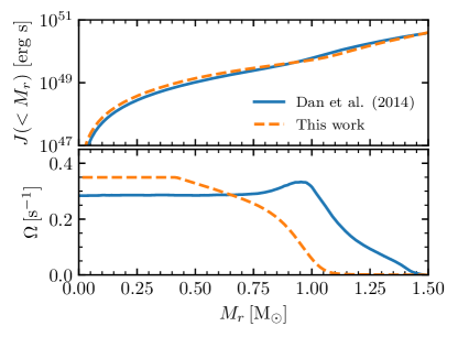
Figure 10: Initial rotation properties for the $q=2/3$, $M_{\rm tot}=1.5\,\mathrm{M}_{\odot}$ MESA model compared to the immediate post-merger rotational properties of the analogous (equipotential-averaged) calculation from Dan et al. (2014). The upper panel shows the total enclosed angular momentum at each mass coordinate. The lower panel shows the angular velocity.

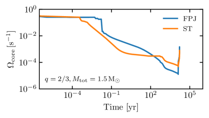
Figure 11: Core rotation rate for the $q=2/3$, $M_{\rm tot}=1.5\,\mathrm{M}_{\odot}$ model assuming two different schemes for angular momentum transport driven by the Tayler instability Tayler (1973). FPJ indicates the scenario and prescription of Fuller et al. (2019); ST is the MESA implementation of the classic Tayler-Spruit dynamo (Spruit, 2002). The core is initialized as shown in Figure 10. In both cases, the core spins down on a timescale shorter than the thermal time in the remnant envelope, so this core spindown occurs before the object has reached the giant phase.

Figure 11 shows the time evolution of the core rotation in a merger model using each of the ST and FPJ treatments. These calculations confirm the essential point that we expect the initially rapidly rotating core to spin down on $\sim$ yr timescales, faster than the remnant can thermally adjust. Therefore, we expect that this spindown energy is deposited in very optically thick material and so primarily goes into work to expand the remnant. This spindown energy from the core will not be significant compared to the energy thermalized during the dynamical and viscous phases of the merger. A rough way to understand this is that the merger thermalized the kinetic energy of the orbit, the orbit and WD rotation have the same period, but the orbital moment of inertia of the binary is much greater than the rotational moment of inertia of the primary WD.

6.2 Giant phase and beyond

In the previous subsection, we argue that the core is unlikely to remain rapidly rotating on kyr timescales. On that first thermal timescale, the remnant swells to become a giant and hence the envelope also no longer need be rapidly rotating because of its large radius.

The remnant may have shed some angular momentum on the way to the giant phase—though our models cannot reliably quantify the amount, as it will depend on the details of the initial thermal and rotational state of the outer layers and the prescriptions for removing mass. During the giant phase, as discussed in Section 4, the remnant presumably loses some mass (and the accompanying angular momentum). However, if it retains even a few percent of the total angular momentum at merger, it will still return to rapid rotation as the envelope starts to cool and the object approaches a compact configuration.

From non-rotating models, we can make a simple estimate of the total angular momentum that an object would be able to retain. We do so by calculating the angular momentum of the object if it were in solid body rotation at the critical rotation rate of the surface: $J_{\rm crit}\equiv I_{\rm NR}\Omega_{\rm crit}$, where $I_{\rm NR}$ is the moment of inertia of the non-rotating model and $\Omega_{\rm crit}=\sqrt{GM/R^{3}}$ is the critical rotation of the surface. (This simple estimate neglects the effects of rotational deformation, the additional outward force from the near-Eddington luminosity, and differential rotation.) The dashed line in the top panel Figure 12 shows this quantity as a function of time in the $q=2/3$, $M_{\rm tot}=1.5\,\mathrm{M}_{\odot}$ MESA model. This quantity generally reaches a minimum as the object crosses to the blue after the giant phase. The middle panel shows the contraction of the radius at this time and the evolution of the quantities that make up $J_{\rm crit}$.

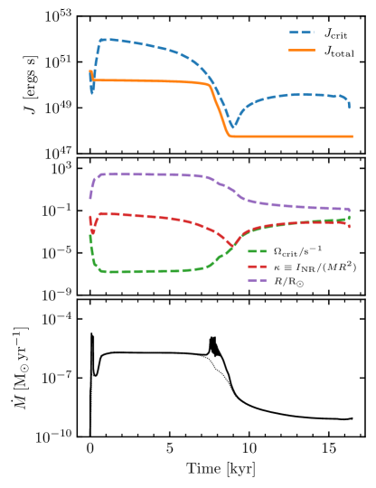
Figure 12: Rotation-related quantities for the evolution of the $q=2/3$, $M_{\rm tot}=1.5\,\mathrm{M}_{\odot}$ MESA model using FPJ angular momentum transport. Dashed lines show quantities from the non-rotating model. In the upper panel, $J_{\rm crit}$ is the critical angular momentum, evaluated as $J_{\rm crit}\equiv I_{\rm NR}\Omega_{\rm crit}$. The middle panel shows these two values individually as well as the remnant radius. In the upper panel, $J_{\rm total}$ is the total angular momentum of the rotating model that sheds its critically-rotating outer layers. The lower panel shows the mass loss rate in this model. The solid line shows the realized mass loss rate in the model while the thin dotted line indicates what the mass loss rate would be if critically-rotating material were not being removed.

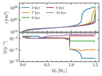
Figure 13: Internal profiles of the models from Figure 12 at indicated times. The top panel shows the specific moment of inertia. The bottom panel shows the angular velocity.

The solid line in the top panel of Figure 12 shows the evolution of the total angular momentum in the rotating $q=2/3$, $M_{\rm tot}=1.5\,\mathrm{M}_{\odot}$ MESA model with the FPJ angular momentum transport prescription. Angular momentum loss occurs such that $J_{\rm total}<J_{\rm crit}$. In addition to a small mass loss rate ($f_{-4}=0.1$), we use built-in MESA capabilities that can, at each timestep, find the mass-loss rate that will keep the star below critical rotation. This approach avoids relying on any particular form for rotationally-enhanced mass loss but still rapidly removes super-critical material from the model. During the evolution $\approx 0.02\,\mathrm{\mathrm{M}_{\odot}}$ of material is shed. The lower panel of Figure 12 shows the mass loss rate in the model as a solid line. The thin, dotted line shows what the mass loss rate would be without this enhancement and there are two clear peaks corresponding to the periods when $J_{\rm total}\sim J_{\rm crit}$. The amount of angular momentum lost during first kyr depends on our initial conditions and so may not be reliable. However, even if all of the angular momentum were retained during this early phase, the object will later shed angular momentum as it goes through the even more restrictive (i.e., lower $J_{\rm crit}$) bottleneck (at 8-10 kyr in Figure 12).

The bottleneck occurs because the star is transitioning from having a significant amount of mass in an extended envelope to a having a more compact configuration. The middle panel of Figure 12 shows the evolution of the dimensionless moment of inertia $\kappa=I/(MR^{2})$, along with $R$ and $\Omega_{\rm crit}$. At fixed mass, $J_{\rm crit}\propto\kappa\sqrt{R}$, and we see the value $R$ monotonically decreases, while the value $\kappa$ displays the minimum. When the star is a giant, there is a significant amount of mass out in the envelope at a radius comparable to the surface radius. Once the star has reached a compact configuration, again, a significant amount of mass is at a radius comparable to the surface radius. However, in between, while the envelope is contracting, there is a smaller fractional amount of mass near the surface. Figure 13 shows information about the internal structure of the remnant at selected times. The top panel plots the specific moment of inertia $i$ (i.e., $I_{\rm NR}=\int i\,dm$). The contribution of the core remains constant (and sub-dominant), but the contribution of material in the envelope ($M_{r}\gtrsim 1.0\,\mathrm{\mathrm{M}_{\odot}}$) changes significantly, reflecting the previously described transition. The bottom panel of Figure 13 shows the profiles of $\Omega$. With the assumed FPJ AM transport, the envelope generally remains near solid body rotation.

Immediately post-merger objects have total angular momentum $J\sim 10^{50}\,\mathrm{erg\,s}$ well above the minimum $J_{\rm crit}$ they will reach in their subsequent evolution. Motivated by Figure 12, we make the assumption that the objects that evolve to the blue (either to collapse to an NS or to go down the WD cooling track) have their total angular momentum reduced to a characteristic value $J_{\rm final}\sim\min J_{\rm crit}$. In our models, $J_{\rm final}\sim 10^{48}\,\mathrm{erg\,s}$. Assuming that subsequent evolution is conservative, this reflects the angular momentum of the final remnant, and so we can estimate the associated rotation periods.

The moment of inertia of a NS is $I\sim 10^{45}\,\mathrm{g\,cm^{2}}$, implying $P_{\rm rot}\sim 10\,\mathrm{ms}$. Figure 14 shows the rotational periods of the subset of models from Figure 9 that likely collapse to NSs. If the merger generates a $\sim 10^{9}\,\mathrm{G}$ field that is then amplified by $\sim 10^{4}$ via flux conservation in the collapse, this could lead to the formation of a millisecond magnetar.

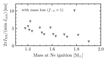
Figure 14: Estimated rotational periods of NSs. Each symbol is one of the subset of models shown in Figure 9 that experience Ne ignition and seem likely to undergo an MIC to form a NS. . Under the assumption of a conservative collapse, the x-axis would approximate the NS (baryonic) mass and the y-axis its rotational period. This simple estimate assumes $I_{\rm NS}=10^{45}\,\mathrm{g\,cm^{2}}$ with no mass dependence.

The moment of inertia of a massive WD is $I\sim 10^{50}\,\mathrm{g\,cm^{2}}$, implying $P_{\rm rot}\sim 10\,\mathrm{min}$. Figure 15 shows the rotational periods of the subset of models from Figure 9 that leave WDs. The rotational periods are mostly in the range $\approx 10-20\,\mathrm{min}$, with the most massive objects at $\gtrsim 1.2\,\mathrm{\mathrm{M}_{\odot}}$ having shorter periods of $\approx 5-10\,\mathrm{min}$. The mass ratio is not explicitly indicated, but increasing mass ratio (at fixed total mass) typically gives higher final masses and shorter periods. We also plot a set of models with less assumed mass loss ($f_{-4}=0.1$) as open symbols. Since the AM bottleneck occurs after the giant phase where the mass loss is most important, the predicted rotational periods do not depend strongly on this choice.

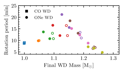
Figure 15: Estimated rotational periods of single WDs on the cooling track. Each solid symbol is one of the subset of models shown in Figure 9 that leave single WDs. The color indicates the total mass at merger via Figure 9. Open symbols are a set of models with lower mass loss $f_{-4}=0.1$. The rotational periods assume that the total angular momentum of the WD is the minimum value of the critical angular momentum encountered in the post-giant-phase evolution of the remnant.

Such periods are much shorter than typical WD rotational periods, which are in the range of hours to days (e.g., Hermes et al., 2017). One class of atypical objects are the hot DQs (Dufour et al., 2008), many of which have photometrically-detected periods (likely associated with rotation) in the range $\approx 5-20\,\mathrm{min}$ (Williams et al., 2016), though one object in this class does have a more typical 2.1 d period (Lawrie et al., 2013) and some do not have detected variability. A few individual objects with rapid rotation are also known. RE J0317-853 has a 12 min rotation period, a $\sim 100$ MG field, and a mass $\approx 1.3\,\mathrm{\mathrm{M}_{\odot}}$. The case for this object as WD-WD merger remnant is somewhat complicated by the fact that it is a DA WD and in orbit with another WD with a roughly similar cooling age (Barstow et al., 1995; Ferrario et al., 1997; Vennes et al., 2003; Külebi et al., 2010). Reding et al. (2020) found the as yet fastest-rotating, apparently isolated WD with a period of $\approx 5.3\,\mathrm{min}$ and a mass $\approx 0.65\,\mathrm{\mathrm{M}_{\odot}}$. Current and future ground- and space-based photometric surveys are expected to enlarge our sample of rapid WD rotators. Our models suggest that a rotation period of $\sim 10\,\mathrm{min}$ in a single WD is a natural signature of its origin in a WD-WD merger.

7 Conclusions

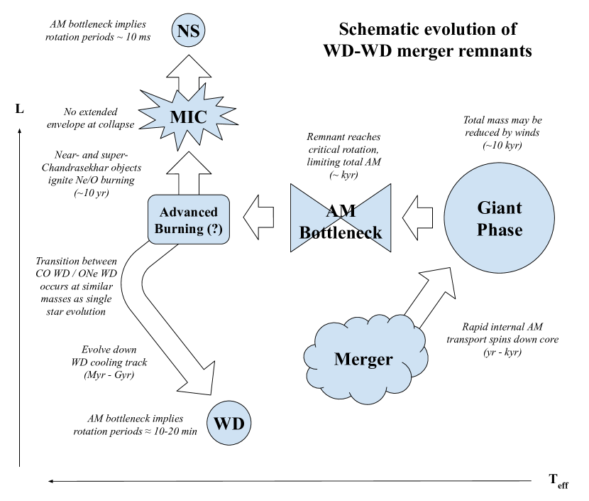
Figure 16: Evolutionary scenario outlined in this work illustrated on a schematic HR diagram. Key phases and corresponding conclusions from this work are indicated.

We construct 1D stellar evolution models of the remnants of the merger of two CO-core WDs using MESA. We use the results of hydrodynamic calculations of the dynamical merger process from Dan et al. (2014), along with the picture of the post-merger viscous phase developed in Shen et al. (2012) and Schwab et al. (2012), to construct approximate initial conditions for merger remnants with a range of total mass and mass ratios. This allows us to survey the possible outcomes for these mergers, extending beyond the single case considered in Schwab et al. (2016), and paying increased attention to cases that leave behind single, massive WDs. This suite of models provides a useful outline of the post-merger evolution. We schematically summarize this evolution and some of our conclusions in Figure 16.

Immediately following the merger, the core of the remnant is rapidly rotating ($\Omega\sim 0.3\,\rm s^{-1}$), reflecting the short orbital period of the tidally-locked binary at merger. When MHD angular momentum transport process are included, we find (in agreement with Shen et al. 2012), that the core spins down on $\sim$ yr timescales, which is much less than the thermal time of the remnant.

On the $\sim$ kyr thermal time, the remnant evolves into a giant. It remains a giant for the $\sim 10$ kyr required to radiate away the thermal energy deposited during the merger. If significant He is present on the WDs at merger (but not detonated), then a stable He-burning shell is set up. This energy release can extend the lifetime of this phase by up to a factor of $\approx 10$, setting up an object similar to an R CrB star, except with a He-deficient, CO-dominated atmosphere. Given the duration, if the Milky Way merger rate of appropriate WD-WD systems is $\sim$ 1 per 300 yr, then we predict the existence of $\sim 30$ galactic objects in this phase.

During the giant phase, the high luminosities, large radii, and metal-rich surface suggest that significant mass loss can occur. This mass loss limits the duration of the giant phase and reduces the mass of the remnant. Simple prescriptions suggest that this is the most non-conservative phase of the post-merger evolution, with the remnant shedding $\sim 0.1\,\mathrm{\mathrm{M}_{\odot}}$ of material. By setting the remnant mass, this phase helps determine whether advanced burning stages occur in the remnant interior and thus influences whether the remnant becomes a NS or WD (and the core composition of the WD).

Our models do not naturally yield ultra-massive CO WDs, that is WDs with CO core compositions and masses significantly above the $\approx 1.06\,\mathrm{\mathrm{M}_{\odot}}$ minimum mass for ONe WDs formed in single star evolution. We find that off-center carbon ignition occurs and converts the core to ONe unless the initial total mass is $\lesssim 1.05\,\mathrm{\mathrm{M}_{\odot}}$ or unless significant mass loss can reduce the mass below this value. We similarly find that Ne ignition occurs in remnants with total masses $\gtrsim\mathrm{M}_{\rm Ch}$ and that in the most cases, the remnant is in a compact, blue configuration at the time collapse to an NS would occur (as also found in Schwab et al., 2016). Only in the most massive remnant we consider (total mass $\approx 1.9\,\mathrm{\mathrm{M}_{\odot}}$) does the collapse to a NS occur in a still-inflated envelope of $\approx 30\,\mathrm{\mathrm{R}_{\odot}}$.

As the remnant evolves blueward and the envelope contracts, we find that an angular momentum “bottleneck” occurs. The assumption of solid body rotation and critical surface rotation define a characteristic total angular momentum for the remnant and this quantity reaches a minimum after the giant phase. Assuming that minimum sets the amount of angular momentum retained by the remnant beyond this point (and that further evolution is conservative), we predict characteristic single WD rotation periods of $\approx 10-20\,\mathrm{min}$. This strengthens the suggestion that single WDs with these rotation periods are the products of WD-WD mergers. For the more massive cases that undergo a merger-induced collapse, NSs formed with this same amount of angular momentum would have periods $\approx 10\,\mathrm{ms}$. These NSs may plausibly have magnetar-strength fields due to the field generated in the aftermath of the merger and its subsequent enhancement during the collapse. As such, WD-WD mergers provide an intriguing pathway for the formation of young magnetars in old stellar populations.

Future calculations that model the WD-WD merger and its immediate aftermath will be of significant utility as they will provide information about which systems experience thermonuclear explosions, and, for the surviving systems, provide higher fidelity initial conditions for the study of the remnant evolution

References

- Asplund et al. (2000) Asplund, M., Gustafsson, B., Lambert, D. L., & Rao, N. K. 2000, A&A, 353, 287
- Barstow et al. (1995) Barstow, M. A., Jordan, S., O’Donoghue, D., et al. 1995, MNRAS, 277, 971, doi: 10.1093/mnras/277.3.971
- Bauer et al. (2020) Bauer, E. B., Schwab, J., Bildsten, L., & Cheng, S. 2020, ApJ, 902, 93, doi: 10.3847/1538-4357/abb5a5
- Benz et al. (1990) Benz, W., Bowers, R. L., Cameron, A. G. W., & Press, W. H. . 1990, ApJ, 348, 647, doi: 10.1086/168273
- Bloecker (1995) Bloecker, T. 1995, A&A, 297, 727
- Cheng et al. (2019) Cheng, S., Cummings, J. D., & Ménard, B. 2019, ApJ, 886, 100, doi: 10.3847/1538-4357/ab4989
- Cheng et al. (2020) Cheng, S., Cummings, J. D., Ménard, B., & Toonen, S. 2020, ApJ, 891, 160, doi: 10.3847/1538-4357/ab733c
- Clayton (2012) Clayton, G. C. 2012, Journal of the American Association of Variable Star Observers (JAAVSO), 40, 539. https://arxiv.org/abs/1206.3448
- Coutu et al. (2019) Coutu, S., Dufour, P., Bergeron, P., et al. 2019, ApJ, 885, 74, doi: 10.3847/1538-4357/ab46b9
- Dan et al. (2015) Dan, M., Guillochon, J., Brüggen, M., Ramirez-Ruiz, E., & Rosswog, S. 2015, MNRAS, 454, 4411, doi: 10.1093/mnras/stv2289
- Dan et al. (2014) Dan, M., Rosswog, S., Brüggen, M., & Podsiadlowski, P. 2014, MNRAS, 438, 14, doi: 10.1093/mnras/stt1766
- Dan et al. (2011) Dan, M., Rosswog, S., Guillochon, J., & Ramirez-Ruiz, E. 2011, ApJ, 737, 89, doi: 10.1088/0004-637X/737/2/89
- Doherty et al. (2015) Doherty, C. L., Gil-Pons, P., Siess, L., Lattanzio, J. C., & Lau, H. H. B. 2015, MNRAS, 446, 2599, doi: 10.1093/mnras/stu2180
- Dufour et al. (2008) Dufour, P., Fontaine, G., Liebert, J., Schmidt, G. D., & Behara, N. 2008, ApJ, 683, 978, doi: 10.1086/589855
- Dunlap & Clemens (2015) Dunlap, B. H., & Clemens, J. C. 2015, in Astronomical Society of the Pacific Conference Series, Vol. 493, 19th European Workshop on White Dwarfs, ed. P. Dufour, P. Bergeron, & G. Fontaine, 547
- Ferrario et al. (1997) Ferrario, L., Vennes, S., Wickramasinghe, D. T., Bailey, J. A., & Christian, D. J. 1997, MNRAS, 292, 205, doi: 10.1093/mnras/292.2.205
- Fuller et al. (2019) Fuller, J., Piro, A. L., & Jermyn, A. S. 2019, MNRAS, 505, doi: 10.1093/mnras/stz514
- García-Berro et al. (2012) García-Berro, E., Lorén-Aguilar, P., Aznar-Siguán, G., et al. 2012, ApJ, 749, 25, doi: 10.1088/0004-637X/749/1/25
- Gourgouliatos & Jeffery (2006) Gourgouliatos, K. N., & Jeffery, C. S. 2006, MNRAS, 371, 1381, doi: 10.1111/j.1365-2966.2006.10780.x
- Gvaramadze et al. (2019) Gvaramadze, V. V., Gräfener, G., Langer, N., et al. 2019, Nature, 569, 684, doi: 10.1038/s41586-019-1216-1
- Heger et al. (2005) Heger, A., Woosley, S. E., & Spruit, H. C. 2005, ApJ, 626, 350, doi: 10.1086/429868
- Hermes et al. (2017) Hermes, J. J., Gänsicke, B. T., Kawaler, S. D., et al. 2017, ApJS, 232, 23, doi: 10.3847/1538-4365/aa8bb5
- Hollands et al. (2020) Hollands, M. A., Tremblay, P. E., Gänsicke, B. T., et al. 2020, Nature Astronomy, 4, 663, doi: 10.1038/s41550-020-1028-0
- Iben & Tutukov (1985) Iben, Jr., I., & Tutukov, A. V. 1985, ApJS, 58, 661, doi: 10.1086/191054
- Iglesias & Rogers (1993) Iglesias, C. A., & Rogers, F. J. 1993, ApJ, 412, 752, doi: 10.1086/172958
- Iglesias & Rogers (1996) —. 1996, ApJ, 464, 943, doi: 10.1086/177381
- Jeffery (1988) Jeffery, C. S. 1988, MNRAS, 235, 1287, doi: 10.1093/mnras/235.4.1287
- Ji et al. (2013) Ji, S., Fisher, R. T., García-Berro, E., et al. 2013, ApJ, 773, 136, doi: 10.1088/0004-637X/773/2/136
- Kashiyama et al. (2019) Kashiyama, K., Fujisawa, K., & Shigeyama, T. 2019, ApJ, 887, 39, doi: 10.3847/1538-4357/ab4e97
- Kawai et al. (1987) Kawai, Y., Saio, H., & Nomoto, K. 1987, ApJ, 315, 229, doi: 10.1086/165126
- Koester & Kepler (2019) Koester, D., & Kepler, S. O. 2019, A&A, 628, A102, doi: 10.1051/0004-6361/201935946
- Külebi et al. (2010) Külebi, B., Jordan, S., Nelan, E., Bastian, U., & Altmann, M. 2010, A&A, 524, A36, doi: 10.1051/0004-6361/201015237
- Lawrie et al. (2013) Lawrie, K. A., Burleigh, M. R., Dufour, P., & Hodgkin, S. T. 2013, MNRAS, 433, 1599, doi: 10.1093/mnras/stt832
- Lorén-Aguilar et al. (2009) Lorén-Aguilar, P., Isern, J., & García-Berro, E. 2009, A&A, 500, 1193, doi: 10.1051/0004-6361/200811060
- Montiel et al. (2015) Montiel, E. J., Clayton, G. C., Marcello, D. C., & Lockman, F. J. 2015, AJ, 150, 14, doi: 10.1088/0004-6256/150/1/14
- Montiel et al. (2018) Montiel, E. J., Clayton, G. C., Sugerman, B. E. K., et al. 2018, AJ, 156, 148, doi: 10.3847/1538-3881/aad772
- Murai et al. (1968) Murai, T., Sugimoto, D., Hōshi, R., & Hayashi, C. 1968, Progress of Theoretical Physics, 39, 619, doi: 10.1143/PTP.39.619
- Nomoto & Iben (1985) Nomoto, K., & Iben, Jr., I. 1985, ApJ, 297, 531, doi: 10.1086/163547
- Paxton et al. (2011) Paxton, B., Bildsten, L., Dotter, A., et al. 2011, ApJS, 192, 3, doi: 10.1088/0067-0049/192/1/3
- Paxton et al. (2013) Paxton, B., Cantiello, M., Arras, P., et al. 2013, ApJS, 208, 4, doi: 10.1088/0067-0049/208/1/4
- Paxton et al. (2015) Paxton, B., Marchant, P., Schwab, J., et al. 2015, ApJS, 220, 15, doi: 10.1088/0067-0049/220/1/15
- Paxton et al. (2018) Paxton, B., Schwab, J., Bauer, E. B., et al. 2018, ApJS, 234, 34, doi: 10.3847/1538-4365/aaa5a8
- Paxton et al. (2019) Paxton, B., Smolec, R., Schwab, J., et al. 2019, ApJS, 243, 10, doi: 10.3847/1538-4365/ab2241
- Perets et al. (2019) Perets, H. B., Zenati, Y., Toonen, S., & Bobrick, A. 2019, arXiv e-prints, arXiv:1910.07532. https://arxiv.org/abs/1910.07532
- Petrovic et al. (2005) Petrovic, J., Langer, N., Yoon, S.-C., & Heger, A. 2005, A&A, 435, 247, doi: 10.1051/0004-6361:20042545
- Reding et al. (2020) Reding, J. S., Hermes, J. J., Vanderbosch, Z., et al. 2020, ApJ, 894, 19, doi: 10.3847/1538-4357/ab8239
- Reimers (1975) Reimers, D. 1975, Memoires of the Societe Royale des Sciences de Liege, 8, 369
- Saio (1988) Saio, H. 1988, MNRAS, 235, 203, doi: 10.1093/mnras/235.1.203
- Saio & Nomoto (1985) Saio, H., & Nomoto, K. 1985, A&A, 150, L21
- Schwab (2018) Schwab, J. 2018, MNRAS, 476, 5303, doi: 10.1093/mnras/sty586
- Schwab (2019) —. 2019, ApJ, 885, 27, doi: 10.3847/1538-4357/ab425d
- Schwab et al. (2016) Schwab, J., Quataert, E., & Kasen, D. 2016, MNRAS, 463, 3461, doi: 10.1093/mnras/stw2249
- Schwab et al. (2012) Schwab, J., Shen, K. J., Quataert, E., Dan, M., & Rosswog, S. 2012, MNRAS, 427, 190, doi: 10.1111/j.1365-2966.2012.21993.x
- Segretain et al. (1997) Segretain, L., Chabrier, G., & Mochkovitch, R. 1997, ApJ, 481, 355, doi: 10.1086/304015
- Shen et al. (2012) Shen, K. J., Bildsten, L., Kasen, D., & Quataert, E. 2012, ApJ, 748, 35, doi: 10.1088/0004-637X/748/1/35
- Shen et al. (2018) Shen, K. J., Boubert, D., Gänsicke, B. T., et al. 2018, ApJ, 865, 15, doi: 10.3847/1538-4357/aad55b
- Spruit (2002) Spruit, H. C. 2002, A&A, 381, 923, doi: 10.1051/0004-6361:20011465
- Staff et al. (2018) Staff, J. E., Wiggins, B., Marcello, D., et al. 2018, ApJ, 862, 74, doi: 10.3847/1538-4357/aaca3d
- Tauris et al. (2015) Tauris, T. M., Langer, N., & Podsiadlowski, P. 2015, MNRAS, 451, 2123, doi: 10.1093/mnras/stv990
- Tayler (1973) Tayler, R. J. 1973, MNRAS, 161, 365
- Timmes & Swesty (2000) Timmes, F. X., & Swesty, F. D. 2000, ApJS, 126, 501, doi: 10.1086/313304
- Timmes et al. (1994) Timmes, F. X., Woosley, S. E., & Taam, R. E. 1994, ApJ, 420, 348, doi: 10.1086/173565
- Tremblay et al. (2019) Tremblay, P.-E., Fontaine, G., Fusillo, N. P. G., et al. 2019, Nature, 565, 202, doi: 10.1038/s41586-018-0791-x
- van Kerkwijk et al. (2010) van Kerkwijk, M. H., Chang, P., & Justham, S. 2010, ApJ, 722, L157, doi: 10.1088/2041-8205/722/2/L157
- Vennes et al. (2003) Vennes, S., Schmidt, G. D., Ferrario, L., et al. 2003, ApJ, 593, 1040, doi: 10.1086/376728
- Webbink (1984) Webbink, R. F. 1984, ApJ, 277, 355, doi: 10.1086/161701
- Williams et al. (2016) Williams, K. A., Montgomery, M. H., Winget, D. E., Falcon, R. E., & Bierwagen, M. 2016, ApJ, 817, 27, doi: 10.3847/0004-637X/817/1/27
- Woosley & Heger (2015) Woosley, S. E., & Heger, A. 2015, ApJ, 810, 34, doi: 10.1088/0004-637X/810/1/34
- Yoon et al. (2007) Yoon, S.-C., Podsiadlowski, P., & Rosswog, S. 2007, MNRAS, 380, 933, doi: 10.1111/j.1365-2966.2007.12161.x
- Zenati et al. (2019) Zenati, Y., Toonen, S., & Perets, H. B. 2019, MNRAS, 482, 1135, doi: 10.1093/mnras/sty2723