Accelerating combinatorial filter reduction through constraints

Abstract

Reduction of combinatorial filters involves compressing state representations that robots use. Such optimization arises in automating the construction of minimalist robots. But exact combinatorial filter reduction is an NP-complete problem and all current techniques are either inexact or formalized with exponentially many constraints. This paper proposes a new formalization needing only a polynomial number of constraints, and characterizes these constraints in three different forms: nonlinear, linear, and conjunctive normal form. Empirical results show that constraints in conjunctive normal form capture the problem most effectively, leading to a method that outperforms the others. Further examination indicates that a substantial proportion of constraints remain inactive during iterative filter reduction. To leverage this observation, we introduce just-in-time generation of such constraints, which yields improvements in efficiency and has the potential to minimize large filters.

I Introduction

A growing body of work has described tools, employed optimization methods, or proposed new algorithms to help automate the design and/or fabrication of robots (e.g., [1, 2, 3, 4, 5]). Important among those approaches are algorithms that aim to manage or minimize resources (for instance, see [6]). Memory is one resource of particular interest to us, not because RAM is expensive, but rather because when state requirements are reduced this often conveys insight into the fundamental informational structure of particular robot tasks (cf. [7, 8]). To this end, we focus on filter reduction, targeting combinatorial filters of the style promoted by LaValle [9]. These filters are discrete variants of the probabilistic estimators ubiquitous in modern robotics, and they yield particularly elegant treatments for certain practical tasks (e.g, see [10]). The minimization problem for combinatorial filters is simple to state and easy to grasp, but continued work on the topic [11, 12, 13, 14, 15, 16] shows that it involves more than first meets the eye.

As a simple example to motivate filter minimization, consider the safari park with vehicle rental service shown in Figure 1(a). The cars for hire are each equipped with a compass and an intelligent gear shifting system. The compass measures the heading of the vehicle before and after its movement, e.g., ‘nw’ means that the vehicle was heading north and then turned to face west. The intelligent gear shifting system takes the readings from the compass as input, and automatically shifts gears to abide with the speed limit. There are three types of speed limits on roads: ($a$) between $15$ and $30$ (gray), ($b$) speeds below $30$ (brown), or ($c$) slower than $15$ (green). Every vehicle is capable of moving with a low gear to drive with a maximum speed $15$, and with a high gear to drive between speed $15$ and $30$. A naïve gear shifting system satisfying the speed limits is realized by a filter shown in Figure 1(b): each vertex represents a system state, each edge represents the state transition, with the label on the edges representing the readings from the compass. A vertex is colored gray if the system outputs high gear, colored green if it outputs low gear, or colored both colors if the system may use either gear (via, say, a nondeterministic choice). We are interested in finding a minimal filter, like the one shown in Figure 1(c), that realizes appropriate behavior but with fewest states.

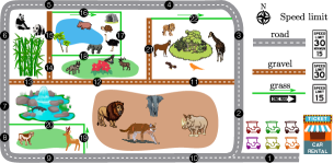
(a)

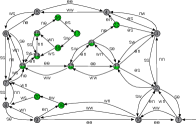
(b)

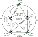
(c)

Figure 1: (a) A safari park with vehicles for rental. The vehicles are equipped with an intelligent gear shifting system automatically shifts the gear to satisfy the speed limit according to its compass readings. (b) A naïve filter to implement the intelligent gear shifting system. (c) A minimal filter for the intelligent gear shifting system.

A natural way to proceed is by first constructing a discrete state-transition system (such as in Figure 1(b)) using the problem description as a basis. Then, the next step is to apply some algorithm capable of compressing it. Despite the apparent similarity of combinatorial filter minimization to the problem of state minimization of deterministic automata, with Myhill–Nerode’s famous and efficient reduction [17], minimization of combinatorial filters is NP-complete [11]. One thread of work studies filter minimization based on merger operations. These algorithms reduce filter minimization to a graph coloring instance [11, 12, 13] or integer linear programming [16]. Saberifar et. al. [13] examined special cases, approximation and parameterized complexity of filter minimization. Rahmani and O’Kane [14] showed that the well-known notion of bisimulation relation in general yields only sub-optimal solutions. They proposed three different integer linear programming formulations to search for the smallest equivalence relation [16]. Recent work shows that both merge and split operations are necessary to find a minimal filter [15]. It formalizes the problem as a clique cover problem subject to the constraint that the output filter should be deterministic and must simulate the output of the input filter. But both criteria involve constraints that are exponential in size, which is obviously computationally unattractive.

In this paper, we propose a new, competing formulation of the filter minimization problem with only a polynomial number of constraints and which yields a concise nonlinear integer programming formulation. Since employing nonlinear constraints is generally computationally inefficient, we ‘flatten’ these nonlinear constraints leading to (1) an integer linear programming and (2) a Boolean satisfaction formalism—both involve expressions of constraints that are of comparable size. Looking at the experimental results in depth, we observed that many constraints remain inactive during the iterative search for a minimal filter. To speed computation within the Boolean satisfaction formalism, we treat these constraints just-in-time: only introducing a constraint when we detect that some proposed variable assignment would violate it. Empirical results show that the speedup from this treatment can outweigh the overhead of detecting and dynamically introducing the constraints.

After presenting the problem statement in Section II, we first formalize filter minimization as an integer nonlinear program in Section III. Based on that, we give integer linear programming and Boolean satisfaction formulations in Section IV. Experimental results appear in Section V.

II Problem Description

II-A Combinatorial filters and their minimization

We firstly recall the notion of a combinatorial filter:

Definition 1 (procrustean filter [18]).

A procrustean filter, p-filter or filter for short, is a 6-tuple $(V,V_{0},Y,\tau,C,c)$ in which $V$ is a non-empty finite set of states, $V_{0}$ is the set of initial states, $Y$ is the set of observations, $\tau:V\times V\rightarrow 2^{Y}$ is the transition function, $C$ is the set of outputs (colors), and $c:V\to 2^{C}\setminus\{\varnothing\}$ is the output function.

The sets of states, initial states, and observations for filter $F$ are denoted $V(F)$, $V_{0}(F)$ and $Y(F)$, respectively. Without loss of generality, we treat a filter as a graph with states as its vertices and transitions as directed edges.

Given a filter $F=(V,V_{0},Y,\tau,C,c)$, an observation sequence (or a string) $s=y_{1}y_{2}\dots y_{n}\in Y^{*}$, and states $v,w\in V$, we say that $w$ is reached by $s$ (or $s$ reaches $w$) when traced from $v$, if there exists a sequence of states $w_{0},w_{1},\dots,w_{n}$ in $F$, such that $w_{0}=v$, $w_{n}=w$, and $\forall i\in\{1,2,\dots,n\},y_{i}\in\tau(w_{i-1},w_{i})$. We denote the set of all states reached by $s$ from a state $v$ in $F$ with $\mathcal{V}_{F}(v,s)$ (also called $s$-children of $v$), and denote all states reached by $s$ from any initial state of the filter with $\mathcal{V}_{F}(s)$, i.e., $\mathcal{V}_{F}(s)=\bigcup_{v_{0}\in V_{0}}\mathcal{V}_{F}(v_{0},s)$. If $\mathcal{V}_{F}(v,s)=\varnothing$, then we say that string $s$ crashes in $F$ starting from $v$. We also denote the set of all strings reaching $w$ from some initial state in $F$ as $\mathcal{S}^{F}_{w}=\{s\in Y^{*}|w\in\mathcal{V}_{F}(s)\}$. The set of all strings that do not crash in $F$ is called the interaction language (or, briefly, just language) of $F$, and is written as $\mathcal{L}(F)=\{s\in Y^{*}|\mathcal{V}_{F}(s)\neq\varnothing\}$. We also use $\mathcal{C}(F,s)$ to denote the set of outputs for all states reached in $F$ by $s$, i.e., $\mathcal{C}(F,s)=\cup_{v\in\mathcal{V}(F,s)}c(v)$. For empty string $\epsilon$, we have $\mathcal{C}(F,\epsilon)=\cup_{v_{0}\in V_{0}}c(v_{0})$.

Definition 2 (output simulating).

Let $F$ and $F^{\prime}$ be two filters, then $F^{\prime}$ output simulates $F$ if $\forall s\in\mathcal{L}(F)$, $\mathcal{C}(F^{\prime},s)\neq\varnothing$ and $\mathcal{C}(F^{\prime},s)\subseteq\mathcal{C}(F,s)$.

Informally, one filter output simulates another if it admits all strings from the other filter and does not generate any new outputs for each of those strings.

We focus on filters with deterministic behavior:

Definition 3 (deterministic).

A filter $F=(V,V_{0},Y,\tau,C,c)$ is deterministic or state-determined, if $|V_{0}|=1$, and for every $v_{1},v_{2},v_{3}\in V$ with $v_{2}\neq v_{3}$, $\tau(v_{1},v_{2})\cap\tau(v_{1},v_{3})=\varnothing$. Otherwise, we say that the filter is non-deterministic.

Algorithm $2$ in [19] can be used to make any non-deterministic filter into a deterministic one. Then the filter minimization problem can be formalized as follows:

Problem: Filter Minimization (fm) Input: A deterministic filter $F$. Output: A deterministic filter $F^{\dagger}$ with fewest states, such that $F^{\dagger}$ output simulates $F$.

We have also a filter reduction problem as follows.

Problem: $k$-Filter Reduction ($k$-fm) Input: A deterministic filter $F$. Output: A deterministic filter $F^{\dagger}$ with no more than $k$ states, such that $F^{\dagger}$ output simulates $F$.

From now on, by filter we mean a deterministic filter, and we shall also assume $F$ has no unreachable states.

III Nonlinear integer programming formulation

In our previous work [15], we expressed the two requirements on the output, namely being both deterministic and output simulating of $F$, via compatibility relationships which characterize all sets of states that can be merged. But since the set of compatibility relationships can be exponentially large, they are time-inefficient to enumerate and space-inefficient to represent explicitly. Hence, in this section, we aim for concision: instead of enumerating compatibility relationships, we represent filters via vertex covers. These covers can be encoded with a polynomial number of binary variables, they allow for determinism and output simulation requirements to be expressed, and they allow us to solve fm as an instance of an integer nonlinear program.

III-A The vertex cover representation of a filter

To begin, define the basic combinatorial object involved:

Definition 4 (vertex cover).

A vertex cover $\bm{K}=\{K_{1},K_{2},\dots,K_{m}\}$ on a filter $F$ is a collection of subsets of vertices which cover all $F$’s vertices, i.e., $K_{i}\subseteq V(F)$ for each $i$, and $\bigcup_{i=1}^{m}K_{i}=V(F)$. The size of $\bm{K}$ is number of the subsets, i.e., $|\bm{K}|=m$.

A vertex cover $\bm{K}=\{K_{1},K_{2},\dots,K_{m}\}$ on filter $F$ is zipped if for every subset $K_{i}\in\bm{K}$ and for each observation $y\in Y(F)$, there exists at least one subset $K_{j}\in\bm{K}$ that contains all $y$-children of the states within $K_{i}$. Next, we show how a zipped vertex cover begets a filter.

Definition 5 (induced filter).

Given a zipped vertex cover $\bm{K}=\{K_{1},K_{2},\dots\}$ on $F=(V,\{v_{0}\},Y,\tau,C,c)$, its induced filter $F^{\dagger}=(V^{\dagger},\{v^{\dagger}_{0}\},Y,\tau^{\dagger},C,c^{\dagger})$ is constructed as follows:

1. Create a state $v^{\dagger}_{i}$ in $F^{\dagger}$ for each non-empty subset $K_{i}$.

2. Select an arbitrary vertex $v^{\dagger}_{i}$ as $v^{\dagger}_{0}$, such that the corresponding $K_{i}$ contains the initial state $v_{0}$ in $F$.

3. For each vertex $v^{\dagger}_{i}$ and $y\in Y$, if $y$-children of vertices in $K_{i}$ is not empty, then add one transition from $v^{\dagger}_{i}$ to $v^{\dagger}_{j}$ under $y$ such that $K_{j}$ contains all $y$-children of $K_{i}$; if there are multiple such $v^{\dagger}_{j}$s, pick an arbitrary one.

4. Assign the output for $v^{\dagger}_{i}$ to be $c^{\dagger}(v^{\dagger}_{i})\in\bigcap_{v\in K_{i}}c(v)$, i.e., an output common to all vertices in $K_{i}$.

Note that each vertex in filter $F$ may be contained in multiple subsets in the vertex cover, and that each subset in the cover is mapped to a unique vertex in the induced filter. Hence, we say that each vertex in $F$ may be mapped to multiple vertices in the induced filter.

The construction does not shrink the filter’s language.

Lemma 1.

Let $F^{\dagger}$ be the induced filter for a zipped vertex cover $\bm{K}$ on a filter $F$. It holds that $\mathcal{L}(F)\subseteq\mathcal{L}(F^{\dagger})$.

Proof sketch.

This lemma can be proved by induction on the length of strings $s\in L(F)$ that shows if $s$ reaches a state $v$ in $F$, then $s$ reaches a state $v^{\dagger}_{i}$ in $F^{\dagger}$ such that the corresponding $K_{i}$ contains $v$. This will show that if $s\in\mathcal{L}(F)$, then $s\in\mathcal{L}(F^{\dagger})$, meaning that $\mathcal{L}(F)\subseteq\mathcal{L}(F^{\dagger})$. ∎

The next throws light on why vertex covers interest us.

Lemma 2.

Given an input filter $F=(V,\{v_{0}\},Y,\tau,C,c)$, if there exists a solution to $k$-fm, then there is always a filter $F^{\dagger}$ as a solution to $k$-fm such that $F^{\dagger}$ is induced from a zipped vertex cover on $F$.

Proof.

Let $F^{\star}=(V^{\star},\{v^{\star}_{0}\},Y,\tau^{\star},C,c^{\star})$ be any solution to $k$-fm with input $F$. From $F^{\star}$ and $F$, we construct a zipped vertex cover $\bm{K}$ on $F$, then construct an induced filter $F^{\dagger}$ from $\bm{K}$ and show that $F^{\dagger}$ is also a solution for $k$-fm.

We construct $\bm{K}$ as follows: For each $i\in\{1,2,\ldots,|V^{\star}|\}$, we choose $v^{\star}_{i}\in V^{\star}$ and let $K_{i}=\{v\in V\mid\mathcal{S}^{F}_{v}\cap\mathcal{S}^{F^{\star}}_{v^{\star}_{i}}\neq\varnothing\}$. Then we set $\bm{K}=\{K_{1},K_{2},\ldots,K_{|V^{\star}|}\}$. Collection $\bm{K}$ is a vertex cover on $F$ because by assumption, $\mathcal{L}(F)\subseteq\mathcal{L}(F^{\star})$, which implies that for each $v\in V$, there is at least one vertex $v^{\star}\in V^{\star}$ such that $\mathcal{S}^{F}_{v}\cap\mathcal{S}^{F^{\star}}_{v^{\star}}\neq\varnothing$, and this means that each vertex $v$ of $F$ is contained in at least one subset $K\in\bm{K}$. In addition, $\bm{K}$ must be zipped. For otherwise, some string is in $F$ but not in $F^{\star}$, which contradicts with the fact that $F^{\star}$ output simulates $F$.

Now, we show that $F^{\dagger}$ is also a solution to $k$-fm. Trivially, $|\bm{K}|=|V^{\star}|\leq k$, and by the construction in Definition 5, $|V(F^{\dagger})|\leq|\bm{K}|$. Hence, $|V(F^{\dagger})|\leq k$.

We will prove by contradiction that $F^{\dagger}$ output simulates $F$. Suppose $F^{\dagger}$ does not output simulate $F$. Then there must be a string $s\in\mathcal{L}(F)$, such that either ($i$) $s\not\in F^{\dagger}$, or ($ii$) at least two states are reached by $s$ in $F^{\dagger}$ ($F^{\dagger}$ is non-deterministic), or ($iii$) $\mathcal{C}(F^{\dagger},s)\not\subseteq\mathcal{C}(F,s)$. Regarding case ($i$), since $s\in\mathcal{L}(F)$ and $\mathcal{L}(F)\subseteq\mathcal{L}(F^{\star})$, we have $s\in\mathcal{L}(F^{\star})$. Let $v^{\star}_{j}$ be a vertex reached by $s$ in $F^{\star}$. Then $s$ must also reach $v^{\dagger}_{j}$ in $F^{\dagger}$, which indicates that $s\in F^{\dagger}$. Regarding case ($ii$), let $v^{\dagger}_{j}$ and $v^{\dagger}_{l}$ ($j\neq l$) be two states in $F^{\dagger}$ that are reached by $s$. Notice that there is an injective function from the vertices and edges in $F^{\dagger}$ to those in $F^{\star}$. Thus, $s$ must reach two different vertices $v^{\star}_{j}$ and $v^{\star}_{l}$ in $F^{\star}$, which contradicts the fact that $F^{\star}$ is deterministic. Regarding case $(iii)$, there must exist a vertex $v^{\dagger}_{i}$ in $F^{\dagger}$ and a vertex $v$ in $F$ that are both reached by $s$ and that $v^{\dagger}_{i}$ and $v$ have different outputs. But according to the construction of $F^{\dagger}$, $v^{\dagger}_{i}$ must share the same output as $v$. Hence, $F^{\dagger}$ must output simulate $F$. ∎

Hence, to solve fm, we can always look for vertex covers.

III-B Searching over vertex covers via variables

Now we represent a vertex cover with binary variables.

To encode a vertex cover $\bm{K}=\{K_{1},K_{2},\dots K_{m}\}$ on an input filter $F=(V,\{v_{0}\},Y,\tau,C,c)$, we introduce the following binary variables:

• Create a binary variable $R^{i}_{v}$ for each $v\in V$ and each $i\in\{1,2,\dots,|V|\}$, and assign $R^{i}_{v}=1$ if and only if $v$ is contained in $K_{i}$. If $i>|\bm{K}|$, then we view $K_{i}$ as an empty set and set $R^{i}_{v}=0$ for all $v\in V$.

• Create a binary variable $q^{i}$ for each $i\in\{1,2,\dots,|V|\}$, and assign $q^{i}=1$ if and only if $K_{i}$ is not empty.

We also define additional variables with constant values assigned from the structure of the input filter:

• Introduce a binary variable $t^{y}_{v}$ for each $v\in V$ and $y\in Y$, to which we assign value $1$ if and only if $v$ has non-empty $y$-children.

• Introduce a binary variable $p^{o}_{v}$ for each $v\in V$ and $o\in O$, to which we assign value $1$ if and only if $v$ has $o$ in its outputs, i.e., $o\in c(v)$.

With these variables, we can encode an output filter and the constraints for it to be a valid solution in fm.

III-C fm as an integer nonlinear program (INP)

Now, we formalize fm as an integer nonlinear program. In what follows, we denote the input filter as $F=(V,\{v_{0}\},Y,\tau,C,c)$, the vertex cover to be searched for as $\bm{K}$, and the induced output filter from $\bm{K}$ as $F^{\dagger}=(V^{\dagger},\{v^{\dagger}_{0}\},Y,\tau^{\dagger},C,c^{\dagger})$. For brevity, we will simply write $\forall i$ for $\forall i\in\{1,2,\dots,|V|\}$, $\forall v$ for $\forall v\in V$, and $\forall y$ for $\forall y\in Y$.

Minimize $$\sum_{1\leq j\leq|V|}q^{j}$$ (INP-Obj) Subject to: $$q^{i},R_{v}^{i}\in\{0,1\}:\forall i,\forall v$$ (INP-Vars) $$R^{i}_{v}\leq q^{i}:\forall i,\forall v$$ (INP-NESubset) $$q^{i}\leq q^{i-1}:\forall i$$ (INP-Sym) $$\sum_{1\leq j\leq|V|}R^{j}_{v_{0}}\geq 1$$ (INP-ValidCover) $\displaystyle{\sum_{1\leq j\leq|V|}\prod_{v\in V}(2-R^{i}_{v}-t^{y}_{v}+R^{j}_{v_{y}})\geq 1:\forall i,\forall y}$ (INP-Zip) $$\small\sum_{o\in C}\prod_{v\in V}(1-R^{i}_{v}+p^{o}_{v})\geq 1:\forall i$$ (INP-Out)

The objective (INP-Obj) is to minimize the number of non-empty subsets in $\bm{K}$. For each $j$, variable $q^{j}$ receives value $1$ if at least one vertex of $F$ is assigned to $K_{j}$. This is expressed by constraints (INP-NESubset). We use the idea of Méndez-Díaz and Paula [20] to reduce symmetry by pushing the non-empty subsets to smaller indices. This is imposed by constraints (INP-Sym).

Constraint (INP-ValidCover) requires that the initial state of $F$ be contained in at least one subset of the vertex cover. Together with constraints (INP-Zip), this ensures that all vertices of $F$ that are reachable from the initial state will be covered by $\bm{K}$. For the output filter to be deterministic, for each observation $y$ and each state $v^{\dagger}_{i}$ in $F^{\dagger}$, $v^{\dagger}_{i}$ must have at most a single $y$-child. Accordingly, for each subset $K_{i}$, there must exist a subset $K_{j}$ that contains all the $y$-children of $K_{i}$. More exactly, $\forall i\in\{1,2,\dots,|V|\}$, $\forall y\in Y$:

$$\exists j\in\{1,2,\dots,|V|\},\text{s.t.},\underbrace{\forall v\in V,\left((R_{v}^{i}t_{v}^{y}=1)\implies(R^{j}_{v_{y}}=1)\right)}_{\text{\footnotesize all $y$-children of $K_{i}$ are contained in $K_{j}$}}.$$

In algebraically simplified form, this is the zipped constraints (INP-Zip). Note that we allow multiple such $K_{j}$’s to exist for any $K_{i}$ and $y$, but in the output filter, only one will be (arbitrarily) picked for the transition.

In addition, the output for vertex $v^{\dagger}_{i}$ should be the common output of all vertices in the subset $K_{i}$. This means that for each subset $K_{i}$, all states within that subset must share a common output. Formally, $\forall i\in\{1,2,\dots,|V|\}$,

$$\exists o\in C,s.t.,\underbrace{\forall v\in V,\left((R_{v}^{i}=1)\implies(p_{v}^{o}=1)\right)}_{\text{\footnotesize all vertices in $K_{i}$ must share output $o$}},$$

which is expressed by constraints (INP-Out).

With a solution to the integer nonlinear program in hand, we first form the vertex cover $\bm{K}$ by constructing the subsets according to the values assigned to variables $R_{v}^{i}$’s. Then we make the output filter $F^{\dagger}$ by following Definition 5.

The next we prove the correctness of INP.

Lemma 3 (correctness).

Let $\bm{K}$ be the vertex cover formed by an optimal solution to the integer nonlinear program for an input filter $F$ and let $F^{\dagger}$ be an induced filter from $\bm{K}$. Filter $F^{\dagger}$ is an optimal solution to fm with input $F$.

Proof sketch.

The constraints from the nonlinear programming formalize exactly the induced filter $F^{\dagger}$ to be deterministic and output simulate the input filter $F$. And the objective function characterizes exactly that $F^{\dagger}$ has the minimum number of states. To show this, we establish the equivalence between the nonlinear constraints and properties of determinism and output simulating in fm. This holds in both directions.

$\impliedby$: If constraints (INP-ValidCover) and (INP-Zip) hold, then $\bm{K}$ is a zipped vertex cover, $F^{\dagger}$ constructed following Definition 5 is deterministic, and $\mathcal{L}(F)\subseteq\mathcal{L}(F^{\dagger})$ as per Lemma 1. If constraint (INP-Out) is satisfied, then $\forall s\in\mathcal{L}(F)$, $\mathcal{C}(F,s)\supseteq\mathcal{C}(F^{\dagger},s)$. Hence, $F^{\dagger}$ is deterministic and output simulates $F$.

$\implies:$ Given an $F^{\dagger}$ that is an optimal solution for fm, construct an induced zipped cover $\bm{K}$ following Lemma 2. The values of the variables encoding this cover must satisfy constraints (INP-NESubset) and (INP-ValidCover). If $F^{\dagger}$ is deterministic, then constraints (INP-Zip) must also be satisfied. The fact that $F^{\dagger}$ output simulates $F$ implies that constraints (INP-Out) are satisfied.

Proof that if $F^{\dagger}$ is minimal, then the value of (INP-Obj) must be optimal (and vice versa) follows similarly. ∎

IV Integer linear programming and SAT

In this section, we introduce three additional formulations of fm: ($i$) an integer linear programming formulation, ($ii$) a Boolean satisfaction formulation, and ($iii$) a Boolean satisfaction with zipped constraints being added just-in-time.

IV-A Integer linear programming (ILP) with linear constraints

This section presents an integer linear program by linearizing the nonlinear constraints (INP-Zip) and (INP-Out).

To linearize constraints (INP-Zip), we introduce a binary variable $a^{i,j}_{y}$ for each $i,j\in\{1,2,\dots,|V|\}$ and $v\in V$ to determine whether there is a transition from vertex $v^{\dagger}_{i}$ to vertex $v^{\dagger}_{j}$ under label $y$ in the output filter $F^{\dagger}$. If $a^{i,j}_{y}=1$, then the value of term $\prod_{v\in V}(1-R^{i}_{v}+1-t^{y}_{v}+R^{j}_{v_{y}})$ must be a positive integer. Otherwise, we choose not to build such a transition in the output filter, regardless of the value of the corresponding term. Mathematically, we have:

$${a^{i,j}_{y}+R^{i}_{v}+t^{y}_{v}-R^{j}_{v_{y}}\leq 2:\forall i,\forall j,\forall v,\forall y}.$$ (ILP-Zip-1)

Then constraints (INP-Zip) are written as

$$\sum_{j=1}^{|V|}a^{i,j}_{y}\geq 1:\forall i,\forall y.$$ (ILP-Zip-2)

For constraints (INP-Out), we similarly introduce a binary variable $b^{i}_{o}$, with value $1$ to denote the fact that the term $\prod_{v\in V}(1-R_{v}^{i}+p^{o}_{v})$ has a positive value. If $b^{i}_{o}=0$, then we do not care whether the value of the corresponding term is positive or not. Thus, we add the following constraints:

$$1-b^{i}_{o}+1-R^{i}_{v}+p^{o}_{v}\geq 1:\forall i,\forall o,\forall v.$$ (ILP-Out-1)

Then constraints (INP-Out) are linearized as follows:

$$\sum_{o\in C}b^{i}_{o}\geq 1:\forall i.$$ (ILP-Out-2)

IV-B Boolean satisfaction (SAT)

We next treat fm as a sequence of $k$-fm problems by enumerating the bound on the output filter size. Each $k$-fm is formalized as a Boolean satisfaction problem, which we call ${SAT}_{[k]}$. To find the minimal filter, the idea is to solve a ${SAT}_{[k]}$, and then decrement $k$ until no smaller output filter can be found.

To obtain a ${SAT}_{[k]}$ instance, we first remove variables $q^{i}$ ($\forall i$) and constraints (INP-NESubset) and (INP-Sym) since we do not need (INP-Obj) and only want to find an output filter with a size bounded by $k$. Next, we treat binary variables $R^{i}_{v}$, $a^{i,j}_{y}$, $b^{i}_{o}$ as boolean-valued and write constraints (ILP-Zip-1)–(ILP-Out-2) in conjunctive normal form (CNF).

Given a filter minimization problem with size bounded by $k$, constraint (INP-ValidCover) is written as a clause:

$$\small\bigvee_{i\in\{1,2,\dots,k\}}R^{i}_{v_{0}}.$$ (SAT-ValidCover)

Constraints (ILP-Zip-1) and (ILP-Zip-2) are written as the following clauses:

$$\overline{a^{i,j}_{y}}\lor\overline{R^{i}_{v}}\lor\overline{t^{y}_{v}}\lor R^{j}_{v_{y}}:\forall i,\forall j,\forall v,\forall y$$ (SAT-Zip-1)

$$\bigvee_{j\in\{1,2,\dots,k\}}a^{i,j}_{y}:\forall i,\forall y.$$ (SAT-Zip-2)

And constraints (ILP-Out-1) and (ILP-Out-2) become:

$$\overline{b^{i}_{o}}\lor\overline{R^{i}_{v}}\lor p^{o}_{v}:\forall i,\forall o,\forall v,$$ (SAT-Out-1)

$$\bigvee_{o\in C}b^{i}_{o}:\forall i.$$ (SAT-Out-2)

Notice that consecutive SAT instances share most of their variables and constraints. The ${SAT}_{[k]}$ instance is equivalent to the ${SAT}_{[k+1]}$ one but with additional unit clauses $\overline{R^{k+1}_{v}}$ for all $v\in V$. Instead of making each ${SAT}_{[k]}$ instance from scratch and solving it, we add unit clauses while decreasing $k$. This allows the solver to re-use knowledge acquired from previous SAT instances, and leads to an incremental anytime procedure in Algorithm 1. First, we initialize $k$ to be $|V(F)|$ (line $1$). Next, we construct a CNF formula for ${SAT}_{[k]}$ and invoke the SAT solver (lines $2$–$6$). If an assignment is found for ${SAT}_{[k]}$ within the time budget (line $7$), then we set its cover choice to be the smallest one found so far (line $8$), update the time budget by the amount of time used in this iteration (line $9$), add the unit clauses (line $10$), and decrease $k$ (line $11$). Otherwise, if the ${SAT}_{[k]}$ has not been solved within the time budget, then we use the minimum cover found so far to construct the minimal filter (line $16$). When given an adequate time budget, the algorithm will find the minimal filter. And running the algorithm for a longer duration increases the chance of finding a smaller filter.

1:  $k\leftarrow|V(F)|$ 2:  $\operatorname{CNF}\leftarrow\operatorname{BuildFormula}(F,k)$ 3:  Initialize minimum vertex cover $\bm{K}_{min}$ to be empty 4:  $solver\leftarrow\operatorname{SATSolver(CNF)}$ 5:  while $k\geq 1$ and $timeout>0$ do 6:     $result\leftarrow solver.\operatorname{solve}(timeout)$ 7:     if $result.solved$ then 8:        $\bm{K}_{min}\leftarrow result.model$ 9:        Reduce $timeout$ by the time used 10:        Add unit clauses $\overline{R^{k}_{v}}$ ($\forall v\in V$) to $solver$ 11:        $k\leftarrow k-1$ 12:     else 13:        break 14:     end if 15:  end while 16:  $F^{\prime}\leftarrow\operatorname{FilterConstruction}(F,\bm{K}_{min})$ 17:  return  $F^{\prime}$

Algorithm 1 $\mathrm{{SAT}}(F,timeout)$

IV-C SAT with just-in-time constraints: LazySAT

In SAT, zipped constraints (SAT-Zip-1) and (SAT-Zip-2) are critical to ensure deterministic transitions between subsets of $\bm{K}$. If a set of vertices in the input filter do not share any common output, then there is no need to check these zipped constraints on any set containing these vertices. In this case, we say that the zipped constraints related to these vertices are inactive. The existence of inactive constraints slows down the resolution of the SAT problem, but detecting and representing all active zipped constraints in fm requires exponential time and space [15]. To speed up the SAT approach without significant overhead, we introduce LazySAT, a just-in-time treatment of the zipped constraints. In LazySAT, we first partition these constraints into non-overlapping sets of clauses, solve the SAT problem without these constraints, and introduce each set of clauses only when a non-zipped cover is returned and it violates these clauses.

Zipped constraints ensure that $\bm{K}$ covers $F$ as well as being zipped. To treat them lazily, we update constraints (SAT-ValidCover) so that every state in $F$ is contained in at least a subset:

$$\bigwedge_{v\in V}\bigg{(}\bigvee_{i\in\{1,2,\dots,k\}}R^{i}_{v}\bigg{)}.$$ (LazySAT-ValidCover)

Next, we partition the clauses in the zipped constraints. Let the set of clauses from constraint (SAT-Zip-1) be $\mathbb{A}$. Then $\mathbb{A}$ can be partitioned into non-overlapping subsets according to the vertex $v$ and outgoing label $y$, i.e., $\mathbb{A}=\cup_{v\in V}\cup_{y}\mathbb{A}^{v}_{y}$. Each subset $\mathbb{A}^{v}_{y}$ consists of the following clauses:

$$\small\bigwedge_{i\in\{1,2,\dots,k\}}\bigwedge_{j\in\{1,2,\dots,k\}}\big{(}\overline{a^{i,j}_{y}}\lor\overline{R^{i}_{v}}\lor\overline{t^{y}_{v}}\lor R^{j}_{v_{y}}\big{)}.$$

Similarly, the set of clauses from constraint (SAT-Zip-2) is denoted as $\mathbb{B}$, which is parameterized by the outgoing label $y$. Each subset $\mathbb{B}_{y}$ consists of the following clauses:

$$\small\bigwedge_{i\in\{1,2,\dots,k\}}\bigg{(}\bigvee_{j\in\{1,2,\dots,k\}}a^{i,j}_{y}\bigg{)}.$$

We detect the violation of these clauses, and add the clauses to the solver as needed. Let $Y_{c}$ be the set of outgoing labels $y$ such that the clauses in $\mathbb{B}_{y}$ are already present in the solver, and $P$ be the set of vertex $v$ and outgoing label $y$ pairs such that $\mathbb{A}^{v}_{y}$ are also added to the solver. Both $Y$ and $P$ are initialized as empty sets. Given a vertex cover $\bm{K}$ returned from the SAT algorithm, if $\bm{K}$ is not zipped, then there must exist a set of states $K\in\bm{K}$ and a label $y$ such that all $y$-children of vertices in $K$ are not contained in any single subset in the cover $\bm{K}$. This must be a consequence of violating some missing clauses parameterized by $K$ and $y$ in the zipped constraints. We add these clauses as follows: ($i$) if $y\not\in Y_{c}$, add $y$ to $Y_{c}$ and add clauses in $\mathbb{B}_{y}$ to the solver; ($ii$) for any $v\in K$, if $(v,y)\not\in P$, add $(v,y)$ to $P$ and add clauses in $\mathbb{A}^{v}_{y}$ to the solver. Now, repeatedly call the solver, adding clauses if needed, until we find a zipped vertex cover with size no greater than $k$. To find a minimum solution, follow the same procedure as Algorithm 1.

V Experimental results

We implemented INP, ILP, SAT and LazySAT in Python, based on mixed integer nonlinear solver SCIP [21], mixed integer linear solver Gurobi [22], and SAT solver CaDiCaL [23]. All executions are conducted on an OSX laptop with a $2.4\text{\,}\mathrm{GHz}$ Intel Core i5 processor, and each algorithm is given $10\text{\,}\mathrm{min}$ budget to solve a filter minimization problem.

First, we minimize the filter in Figure 1(b). INP failed to give a result before timing out, while ILP, SAT and LazySAT give minimal filters with $5$ states within $1\text{\,}\mathrm{s}$, $2\text{\,}\mathrm{s}$ and $100\text{\,}\mathrm{s}$, respectively. One such minimal filter is shown in Figure 1(c). We collected no further results for INP since it appears to be incapable of minimizing filters with more than $10$ states within $10\text{\,}\mathrm{min}$.

To test the performance of the remaining three algorithms, we randomly generated a filter as follows: ($i$) construct a tree with a root node at layer $0$ and $w$ nodes at each of $d$ additional layers, and then connect each vertex from a parent vertex in an earlier layer by drawing a directed edge; ($ii$) randomly pick $m$ vertices to add self loops; ($iii$) randomly pick $n$ vertices to connect to some parent vertex in a later layer, so as to generate cycles. Next we randomly assign $n_{o}$ outputs to vertices in the filter, where each vertex is assigned with $p$ of them. Similarly, we randomly assign $n_{y}$ observations to the edges in the filter while keeping the filter deterministic.

To compare ILP and SAT-based approaches, we start with a filter structure randomly generated by parameters $d$=$4$, $w$=$3$, $m$=$n$=$2$, $p$=$2$ and $n_{o}$=$5$. For any given number of observations $n_{y}$, we sample $10$ filters, and collect the time to minimize these filters for each algorithm in Figure 2(a). As more observations are added to the filter, fewer states share common observations. The zipped constraints (ILP-Zip-1) and (SAT-Zip-1) will be simplified, since $a^{i,j}_{y}$ connects with fewer vertices. Hence, the computational time for both ILP and SAT-based approaches tend to decrease. Fixing the number of observations to be $n_{y}=5$, we also collect the computation time under varying outputs in Figure 2(b). This gives an opposite trend as increasing the number of outputs makes the problem harder from two aspects: ($i$) the number of variables increases; ($ii$) the number of output constraints (ILP-Out-1) or (SAT-Out-1) increases owing to both an increasing number of outputs and an increasing number of vertices with $p^{o}_{v}=0$ for each output $o$. Across both studies, SAT-based approaches outperform integer linear programming. We speculate that this is because the constraints for fm are fundamentally combinatorial in nature and can be concisely encoded in CNF. These CNF constraints can be exploited relatively efficiently (e.g., by building a constraint-dependency graph). And a final factor might be that the objective function really takes a limited range of values and its values can be enumerated efficiently.

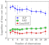
(a) Time cost (natural log) for inputs with varying observations.

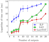
(b) Time cost (natural log) for inputs with varying outputs.

Figure 2: Comparison of logarithmic computational time to minimize filters with different number of outputs and observations.

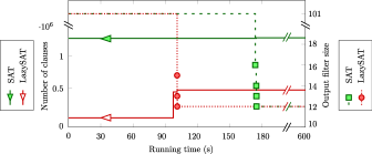
Figure 3: The number of constraints used by SAT and LazySAT to find the sub-optimal solutions while increasing the running time. The input filter is constructed with parameters $d=20$, $w=5$, $m=n=10$, $p=1$, with $50$ observations and $5$ outputs.

Observe that in Figure 2(b), as we increase the number of outputs, LazySAT significantly outperforms SAT since few states share common outputs, so most zipped constraints are inactive and can be removed. We further tested them on a larger filter instance, where many states share common outputs and hence a significant proportion of constraints become active. In Figure 3, instead of presenting the time to find a minimal solution, we report the number of clauses used by the solver, and size of the sub-optimal solutions found by the two algorithms along the way. LazySAT is still able to find sub-optimal solutions faster than SAT, and the number of clauses used by LazySAT is much fewer than those in SAT. Treating constraints lazily does incur overhead in detecting and adding the active clauses, but the speedup from just-in-time treatment is seen to outweigh its overhead even when a large number of vertices share common outputs.

VI Conclusion

This paper accelerates filter minimization through constraints. It introduces a concise constraint description, encodes it in different forms, and reports empirical evidence suggesting that constraints in conjunctive normal form are most efficient. It also proposes a just-in-time treatment of constraints to speed up iterative filter reduction. Future work might consider non-deterministic input, as well as searching for non-deterministic minimizers.

References

- [1] K. S. Luck, J. Campbell, M. Jansen, D. Aukes, and H. B. Amor, “From the lab to the desert: Fast prototyping and learning of robot locomotion,” in Robotics: Science and Systems, Cambridge, Massachusetts, 2017.
- [2] A. Schulz, C. Sung, A. Spielberg, W. Zhao, R. Cheng, E. Grinspun, D. Rus, and W. Matusik, “Interactive robogami: An end-to-end system for design of robots with ground locomotion,” International Journal of Robotics Research, vol. 36, no. 10, pp. 1131–1147, 2017.
- [3] A. M. Hoover and R. S. Fearing, “Fast scale prototyping for folded millirobots,” in Proceedings of IEEE International Conference on Robotics and Automation, Pasadena, California, 2008, pp. 886–892.
- [4] A. Pervan and T. D. Murphey, “Low complexity control policy synthesis for embodied computation in synthetic cells,” in Proceedings of International Workshop on the Algorithmic Foundations of Robotics, Mérida, México, 2018, pp. 602–618.
- [5] Y. Zhang and D. A. Shell, “Abstractions for computing all robotic sensors that suffice to solve a planning problem,” in Proceedings of IEEE International Conference on Robotics and Automation, Paris, France, 2020, pp. 8469–8475.
- [6] A. Censi, “A Class of Co-Design Problems With Cyclic Constraints and Their Solution,” IEEE Robotics and Automation Letters, vol. 2, no. 1, pp. 96–103, 2017.
- [7] J. H. Connell, Minimalist Mobile Robotics: A Colony Style Architecture for an Artificial Creature. San Diego, CA: Academic Press, 1990.
- [8] B. R. Donald, “On Information Invariants in Robotics,” Artificial Intelligence — Special Volume on Computational Research on Interaction and Agency, Part 1, vol. 72, no. 1–2, pp. 217–304, 1995.
- [9] S. M. LaValle, “Sensing and filtering: A fresh perspective based on preimages and information spaces,” Foundations and Trends in Robotics, vol. 1, no. 4, pp. 253–372, 2010.
- [10] B. Tovar, F. Cohen, L. Bobadilla, J. Czarnowski, and S. M. Lavalle, “Combinatorial filters: Sensor beams, obstacles, and possible paths,” ACM Transactions on Sensor Networks (TOSN), vol. 10, no. 3, pp. 1–32, 2014.
- [11] J. M. O’Kane and D. A. Shell, “Automatic reduction of combinatorial filters,” in Proceedings of IEEE International Conference on Robotics and Automation, Karlsruhe, Germany, 2013, pp. 4082–4089.
- [12] J. M. O’Kane and D. A. Shell, “Concise planning and filtering: hardness and algorithms,” IEEE Transactions on Automation Science and Engineering, vol. 14, no. 4, pp. 1666–1681, 2017.
- [13] F. Z. Saberifar, A. Mohades, M. Razzazi, and J. M. O’Kane, “Combinatorial filter reduction: Special cases, approximation, and fixed-parameter tractability,” Journal of Computer and System Sciences, vol. 85, pp. 74–92, 2017.
- [14] H. Rahmani and J. M. O’Kane, “On the relationship between bisimulation and combinatorial filter reduction,” in Proceedings of IEEE International Conference on Robotics and Automation, Brisbane, Australia, 2018, pp. 7314–7321.
- [15] Y. Zhang and D. A. Shell, “Cover combinatorial filters and their minimization problem,” in Proceedings of International Workshop on the Algorithmic Foundations of Robotics, Oulu, Finland, 2020.
- [16] H. Rahmani and J. M. O’Kane, “Integer linear programming formulations of the filter partitioning minimization problem,” Journal of Combinatorial Optimization, vol. 40, pp. 431–453, 2020.
- [17] J. E. Hopcroft, R. Motwani, and J. D. Ullman, Introduction to Automata Theory, Languages, and Computation, 3rd ed. Addison-Wesley, 2006.
- [18] F. Z. Saberifar, S. Ghasemlou, J. M. O’Kane, and D. A. Shell, “Set-labelled filters and sensor transformations.” in Robotics: Science and Systems, Ann Arbor, Michigan, 2016.
- [19] F. Z. Saberifar, S. Ghasemlou, D. A. Shell, and J. M. O’Kane, “Toward a language-theoretic foundation for planning and filtering,” International Journal of Robotics Research—in WAFR’16 special issue, vol. 38, no. 2-3, pp. 236–259, 2019.
- [20] I. Méndez-Díaz and P. Zabala, “A cutting plane algorithm for graph coloring,” Discrete Applied Mathematics, vol. 156, no. 2, pp. 159–179, 2008.
- [21] G. Gamrath, D. Anderson, K. Bestuzheva, W.-K. Chen, L. Eifler, M. Gasse, P. Gemander, A. Gleixner, L. Gottwald, K. Halbig, G. Hendel, C. Hojny, T. Koch, P. Le Bodic, S. J. Maher, F. Matter, M. Miltenberger, E. Mühmer, B. Müller, M. E. Pfetsch, F. Schlösser, F. Serrano, Y. Shinano, C. Tawfik, S. Vigerske, F. Wegscheider, D. Weninger, and J. Witzig, “The SCIP Optimization Suite 7.0,” Zuse Institute Berlin, ZIB-Report 20-10, 2020. [Online]. Available: http://nbn-resolving.de/urn:nbn:de:0297-zib-78023
- [22] LLC Gurobi Optimization, “Gurobi optimizer reference manual,” 2020. [Online]. Available: http://www.gurobi.com
- [23] A. Biere, K. Fazekas, M. Fleury, and M. Heisinger, “CaDiCaL, Kissat, Paracooba, Plingeling and Treengeling entering the SAT Competition 2020,” in Proc. of SAT Competition 2020 – Solver and Benchmark Descriptions, vol. B-2020-1. University of Helsinki, 2020, pp. 51–53.