A search for variable subdwarf B stars in TESS Full Frame Images
I. Variable objects in the southern ecliptic hemisphere

Abstract

We report the results of our search for pulsating subdwarf B stars in Full Frame Images, sampled at 30 min cadence and collected during Year 1 of the TESS mission. Year 1 covers most of the southern ecliptic hemisphere. The sample of objects we checked for pulsations was selected from a subdwarf B stars database available to public. Only two positive detections have been achieved, however, as a by-product of our search we found 1807 variable objects, most of them not classified, hence their specific variability class cannot be confirmed at this stage. Our preliminary discoveries include: two new subdwarf B (sdB) pulsators, 26 variables with known sdB spectra, 83 non-classified pulsating stars, 83 eclipsing binaries (detached and semi-detached), a mix of 1535 pulsators and non-eclipsing binaries, two novae, and 77 variables with known (non-sdB) spectral classification. Among eclipsing binaries we identified two known HW Vir systems and four new candidates. The amplitude spectra of the two sdB pulsators are not rich in modes, but we derive estimates of the modal degree for one of them. In addition, we selected five sdBV candidates for mode identification among 83 pulsators and describe our results based on this preliminary analysis. Further progress will require spectral classification of the newly discovered variable stars, which hopefully include more subdwarf B stars.

1 Introduction

Subdwarf B (sdB) stars are identified as objects located at the blue end of the horizontal branch in the Hertzsprung-Russell diagram (Heber, 2016). These stars are compact in size, with surface gravities, $\log(g/\,\mbox{$\mbox{cm}\,\mbox{s}^{-2}$})$, of 5.0 to 5.8, which translates into radii of 0.15 – 0.35 R_☉. SdBs are blue due to their high effective surface temperature (T_eff) ranging between 20,000 and 40,000 K. Such a high temperature makes them candidates for the ionizing sources of interstellar gas at high galactic latitudes (de Boer, 1985) and mostly responsible for the ultraviolet upturn phenomenon in early-type galaxies (Brown et al., 1997). The sdB stars have masses 0.47 M_☉ on average, which is sometimes called the canonical mass (Heber, 2016).

After the discovery of pulsating sdBs (sdBV) observationally by Kilkenny et al. (1997) and theoretically by Charpinet et al. (1997), asteroseismology became the major tool to investigate the interior of sdBs. The pulsations were found at both low and high frequencies. The low frequencies (long periods of hours) are explained by gravity modes, while the high frequencies (short periods of minutes) are explained by pressure modes Fontaine et al. (2003). Since these stars were discovered only recently, it was essential to make an effort in more discoveries to increase the sample of sdBVs to a statistically significant number. First discoveries were made from the ground and detections were limited to sdBVs showing pressure modes. They were easier to detect because of their higher observable amplitudes and shorter periods. sdBVs with gravity modes were also detected from the ground, but the actual number of these discoveries was never published. Only a handful sdBVs were found to be pulsating in both types of modes, with Balloon 090100001 being the best example (Baran et al., 2005). Overall, there are about 50 sdBVs found only from the ground. Thanks to the Kepler spacecraft (Borucki et al., 2010) we found more sdBVs. Most of them pulsate in gravity modes and many of them show both types of pulsations, which means that hybrid behaviour is common among sdBVs. To date, there are around 130 sdBV found in both ground and space data (Holdsworth et al., 2017; Reed et al., 2018). SdBVs are found in both open (Reed et al., 2012) and globular (Randall et al., 2009) clusters but mostly as Galactic-field counterparts. While ground-based discoveries were made all over the sky, Kepler discoveries were limited, first to the fixed region during the original mission, and second to the ecliptic plane during K2 mission. We lack a complete all-sky search for sdBVs. It prevented us from a comprehensive analysis of pulsation properties correlated with stellar population to conclude the location of instability strip(s) or physical parameters (especially masses).

At present the Kepler successor, the Transiting Exoplanet Survey Satellite (TESS, Ricker et al., 2014) is an all-sky survey whose primary goal is to detect exoplanets orbiting around nearby bright stars using the transit method. As a by-product, time-series photometry of nearly 20,000 additional targets for astrophysical research are produced (pre-defined targets). These data are taken either in the long cadence (LC) or short cadence (SC) modes. The LC is 30 min, while the SC is 2 min. What makes TESS different from Kepler is that full-frame images (FFI) taken with LC are all downloaded and available to public. This is a significant source of time-series data, since almost the entire sky is sampled at the 30 min resolution. Since only for pre-defined targets, time-series data are prepared by the in-house pipeline, the other objects detected in the FFIs need special data processing. Handling all objects detectable in the FFIs, although desirable, is technically difficult (processing would take months if not years), one can focus on a selected target type only, limiting the time needed for data processing and time-series delivery. During Year 1 and 2, TESS covered nearly 85% of the sky. The entire TESS field is divided into 26 sectors and each sector is monitored for 27 days. After first 13 sectors in the southern ecliptic hemisphere were completed, TESS switched to the northern ecliptic hemisphere.

The main goal of our work was to select sdBs and sdB candidates that were not included in the pre-defined target list, produce time-series data directly from FFIs and make mode identifications of the best suitable cases showing pulsations. An all-sky search for sdBVs, along with Gaia parallaxes will tell us about the distribution of these stars in the Galaxy and contribute toward pulsation-stellar population relationship. In Section 2 we describe the source of our targets, the selection process and data processing. In Section 3 we present objects with found variables. Section 4 reports our mode identification effort, followed by Section 5 that summarizes our results.

2 Target selection and flux extraction

We used the sdB database described by Geier (2020) that we consider the most updated database of confirmed sdB as well as sdB candidates. It was prepared based on Gaia mission (Gaia Collaboration, 2018), specifically ESA Gaia Data Release 2 (DR2) and several ground-based multi-band photometry surveys. Color indices, absolute magnitudes and reduced proper motions were used to select the most suitable candidates. The database is limited to Gaia G mag = 19 and contains 39 800 objects. From this sample we selected targets located in the southern ecliptic hemisphere and covered by TESS silicons. Using Gaia IDs and target coordinates we applied TOPCAT (Taylor, 2005) to reject targets that are assigned to be observed in the SC mode. Then, we used Tesscut (Brasseur et al., 2019) to collect sector information targets in our sample will be observed in, and targets with no sector assignment were also rejected. Finally, we filtered targets assigned to sector 1-13 only, and we ended up with 21,879 targets. It turned out that 1237 targets have no useful data, so these were also rejected from our sample, resulting in 20,642 targets. For completeness, we have included targets with non-sdB spectral classification. It may also happen that some of these already classified objects will be reclassified as sdBs with further analysis. In addition, other researchers may find it useful to have these objects identified as variables.

We used the Eleanor (Feinstein et al., 2019) that is an open source python framework developed for downloading, analysis, and visualization of data directly from the TESS FFIs. It is able to extract corrected time-series data for a given object. As input it takes the TIC ID, Gaia ID, or coordinates along with observed TESS sector information, and returns with a table FITS file with time-series data, optimal aperture shape applied.

The Eleanor works in two steps. First, it detects a target and creates a target pixel file (TPF), then it does aperture photometry to extract the flux and create time-series data. Eleanor works directly with the "Barbara A. Mikulski Archive for Space Telescopes" (MAST) to download all necessary data for a given target. We specified a square target mask of 15 pixels on side and a square background mask of 31 pixels on side. It delivers raw and corrected time-series data. The raw data is a simple sky-subtracted simple aperture photometry, which is basically a sum of all flux within an optimal aperture for each timestamp. The corrected data account for known satellite artifacts. We extracted both data sets and have chosen the one that shows better signal to noise ratio. All details on the Eleanor can be found in the reference paper by Feinstein et al. (2019).

We used lightkurve python package (Lightkurve Collaboration et al., 2018) to detrend and remove outliers from both raw and corrected time-series data. We clipped the data at 4$\sigma$ and de-trended long term variations (longer than two days). Then, we cleaned these data again by removing data points that were not clipped, but still significantly deviated from the expected trend. These were data points at the beginning and/or end of each satellite orbit that are caused by unstable satellite temperature. Finally, we normalized fluxes by calculating $(f/\bar{f}-1)*1000$ reporting amplitudes in parts per thousand (ppt). We stress that the Eleanor does not remove contributions from neighboring objects, which results in overestimated average flux and diluted amplitude of flux variations. Therefore, the amplitudes are not realistic and are affected by our case-to-case definition of a flux zero point accurately. In case of sdBV stars, the amplitudes are not important, but accurate modelling of eclipsing binaries or classical pulsators may require further individual effort to pull out the fluxes with preserved amplitudes.

We calculated amplitude spectra for each target and we used them to search for flux variations. These spectra help detect variations even if the time-series data show no significant (by eye) variations. We accept a positive detection only if peaks in the spectra meet our signal-to-noise (S/N) ratio of 4.5 (Baran et al., 2015). Since we work with the long cadence data, the Nyquist frequency equals 277 ${\mu}$Hz (24c/d), which translates to 30 min period. This limits our search to gravity mode sdBVs only.

3 Results of our flux variation search

We detected significant flux variations in 1807 objects, out of which 28 are classified as sdBs, 2 as subdwarfs (sd), 77 as non-sdBs, and 1619 are not spectroscopically classified. To identify sdB objects we used the sdB database Geier (2020), the LAMOST spectroscopic survey (Lei et al., 2018, 2019a, 2019b; Luo et al., 2019), the Evryscope survey (Ratzloff et al., 2020) and the Simbad database (Wenger, M. et al., 2000). The large square pixels, 21 arcsec on side, cause serious issues in crowded regions of the sky, since an optimal aperture may contain neighboring objects. We over-plotted optimal apertures of all our objects, adopted by the Eleanor, on top of the Digitized Sky Survey (DSS) color images using the Aladin (Bonnarel, F. et al., 2000). If the aperture overlaps with additional sources, and we are not positive about which object a flux variation comes from, we made remarks in Tables 1–7 that provide basic information on our target findings and possible contamination. In case an optimal aperture region contains more than five objects we marked it with crowded region remark, while in case the optimal aperture is densely covered by stars, e.g. a cluster region, we marked it with very crowded region. If a few objects (< 5) were spotted, we specified the number of objects within a radius or in case of a single object within optimal aperture, we provided the distance to the object. If possible, we provided designations of such objects. In addition, some of the objects may have already been discovered and published. If we found that a given target is already known as a variable star, we provided a relevant reference. We included these objects for completeness and to report on the frequency of variable stars found in the TESS data.

3.1 SdB stars

We found 28 variable objects classified as sdB and we list them in Table 1. Two objects, Gaia DR2 3129751228471383808 and 3159937564294110080, show multiple peaks in their amplitude spectra (Figure 1), which we interpret as g-modes. Both objects were first observed by Høg et al. (2000) and the spectral classifications were made by Luo et al. (2019) and Lei et al. (2018).

The other 26 objects show light variation typical of binaries. All objects (here and later on) that show mono-periodic, most likely binary, behavior with large amplitude flux variations were phased and the orbital periods were cited in the relevant figures and tables. If a flux variation is easily seen in the light curves we phased and binned data and these are plotted in Figure 2. This figure contains candidates for reflection binaries (a sdB and a low mass main sequence companion) and ellipsoidal binaries (a sdB and a white dwarf). One of the eclipsing binaries, Gaia DR2 2969438206889996160, which has just recently been published by Ratzloff et al. (2020), is an HW Vir system (Wood et al., 1993; Baran et al., 2018).

Figure 3 includes 14 variable sdB stars that show low amplitude variation that are detectable in amplitude spectra. Even though the peaks we detected are in the g-mode region, one or two peaks can be interpreted as either pulsations or binarity. The only exception could be Gaia DR2 599294211494840704 that shows a single peak between 160 and 200 $\upmu$Hz. Gaia DR2 3757498318395098240 shows two peaks above 80 $\upmu$Hz, but the higher frequency peak is a harmonic, hence we claim it to be a signature of binarity, as well.

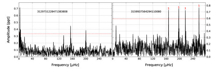
Figure 1: Amplitude spectra of two sdBV stars. Horizontal red dashed line indicates $4.5\,\sigma$ detection threshold (all relevant figures). In the right panel we added our guesses on the modal degree based on the period spacing.

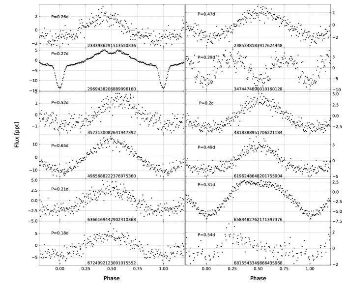
Figure 2: Phased and binned time-series data of a sample of sdBs that show relatively large amplitude flux variations.

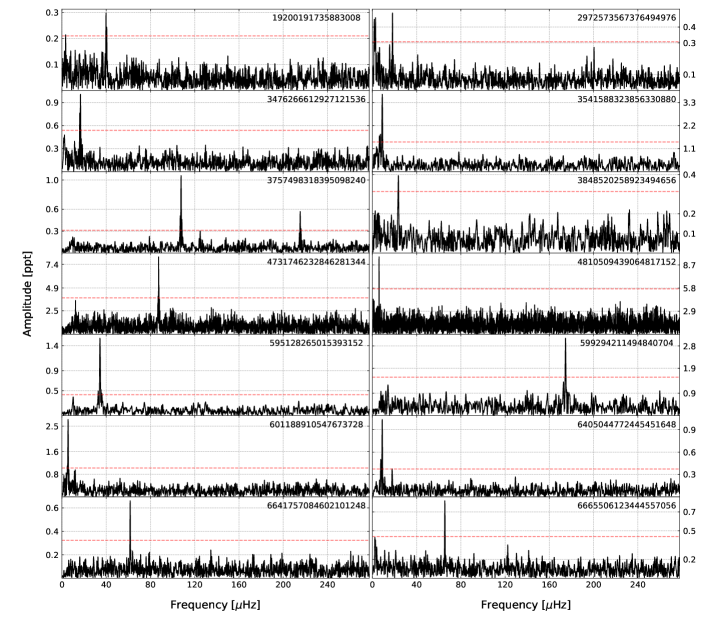
Figure 3: Amplitude spectra of a sample of sdBs that show low amplitude flux variations.

Table 1: Basic information of 28 objects classified as sdBs. Time-series data or amplitude spectra of these objects are plotted in Figs. 1,2 and 3. Objects in all tables and figures are sorted by Gaia ID.

Gaia DR2	TIC	Name	G mag	Sector	Period[d]	Remarks
19200191735883008	337216760	PG 0229+064	11.9242	4	0.2906	-
2333936291513550336	12379252	Ton S138	16.0148	2	0.2648	-
2385348183917624448	9035375	PHL 460	12.2071	2	0.4734	object 1.3’ away
2969438206889996160	139397815	HW Vir type	13.6079	5-6	0.2746	Ratzloff et al. (2020)
2972573567376494976	146340999	EC 04542-2320	16.1603	5	0.6377	-
3129751228471383808	237597052	TYC 161-49-1	11.1375	6	0.05-0.1	sdBV candidate
3159937564294110080	262753627	TYC 770-941-1	12.4615	7	0.04-0.08	sdBV candidate
3474474890010160128	402107174	EC 12067-2747	15.8566	10	0.2923	-
3476266612927121536	443619867	HE 1221-2618	14.6445	10	0.6925	-
3541588323856330880	219512715	EC 11362-2049	14.1469	9	1.2933	-
3573130082641947392	386644511	PG 1145-135	14.2710	9	0.5239	-
3757498318395098240	902644573	PG 1039-119	16.4582	9	0.1075	-
3848520258923494656	275358553	PG 0957+037	15.4126	8	0.4928	-
4731746232846281344	198005084	EC 03572-5455	16.2585	2-4	0.1325	-
4810509439064817152	200323355	EC 05043-4538	16.4590	4-6	1.9133	-
4818388951706221184	77372867	2MASS J04512188-3743059	16.0941	4-5	0.2007	-
4965688222376975360	49593787	-	13.4408	3	0.6467	Vos et al. (2018)
595128265015393152	366656123	2MASS J08412266+0630294	14.8264	7	0.337	-
599294211494840704	366353515	PTF 1J082340.04+081936.5	14.7016	7	0.0663	Kupfer et al. (2017)
601188910547673728	800381314	2MASS J08251803+1131062	14.6493	7	2.0941	Boudreaux et al. (2017)
6196248648201755904	6116091	HE 1318-2111	14.7001	10	0.4879	Kupfer, T. et al. (2015)
6366169442902410368	265124418	JL 24	15.2841	13	0.2091	-
6405044772445451648	234287962	EC 22209-6344	15.3326	1	1.3015	-
6583482762171397376	159735013	CD-3914181	10.9537	1	0.3054	CMC 316837 1.3" away
6641757084602101248	320055780	EC 19301-5523	15.9155	13	0.1878	-
6665506123444557056	1990074078	EC 20043-5310	15.2382	13	0.1767	object 2.6" away
6724092123091015552	86141703	-	13.4682	13	0.1782	Ratzloff et al. (2020)
6815543349866435968	302114308	EC 21271-2412	15.9811	1	0.5418	-

3.2 Pulsators

We found 83 additional objects that show multi-peak amplitude spectra that we interpret as pulsation. These objects are not classified so we cannot make any definite conclusion on their pulsation nature. We listed these objects along with their basic information in Table 2. Objects in this list have at least two peaks in their amplitude spectra that are not related. Some of the objects show peaks at frequencies too low compared to known g-mode sdBVs (e.g. Gaia DR2 5618197551112972288), unless they are very cool sdBVs, which have g-modes shifted to longer periods. We show the amplitude spectra of these pulsators in Figures 4 and 5.

Even though we have no spectral classifications for these pulsator candidates, we selected five objects for preliminary mode identification. We chose objects that are rich in high amplitude peaks in a frequency range that is typical of g-modes in sdBVs. These stars may also be $\delta$ Scuti or $\beta$ Cep stars, however Geier et al. (2019) and Geier (2020) applied a color index criterium to avoid cool stars. These papers provide detailed arguments using Gaia color indices that these targets are hot subluminous stars and occupy the region $-0.7<G_{BP}-G_{RP}\lesssim 0.7$ in the Gaia colour space. Selecting only the targets which are rich in high amplitude peaks are necessary to search for multiplets and equally spaced overtones. The frequencies cannot be too close to the Nyquist frequency, since we are unable to discern between true peaks and their reflections across the Nyquist frequency. This constrains our selection to cool sdBVs, since only these objects have peaks in their amplitude spectra shifted to lower frequencies, as compared with hotter g-mode sdBVs. Even though we are not sure the selected objects are sdBVs, our suggested mode assignment may be useful if a spectral classification is confirmed by future spectroscopic analyses. We show the result of our mode identification in Section 4.

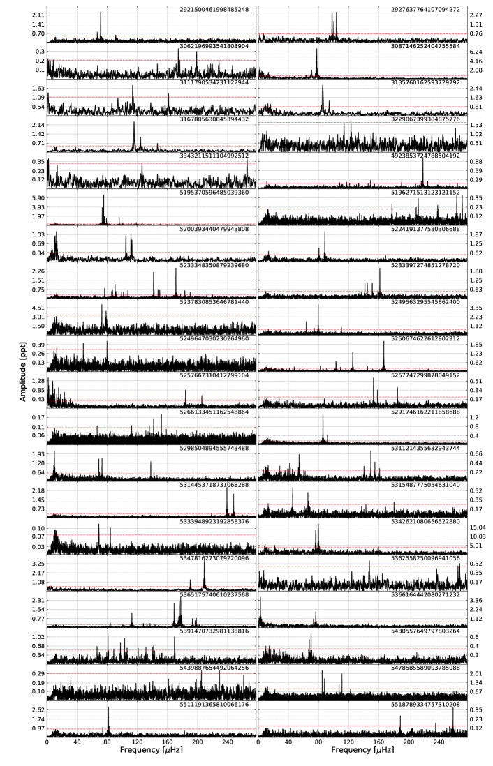
Figure 4: Amplitude spectra of pulsator candidates that are not spectroscopically classified.

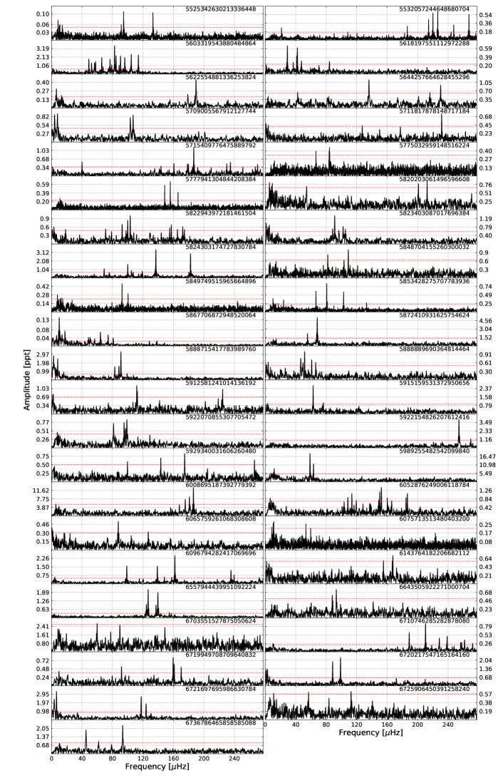
Figure 5: Same as Figure 4

Table 2: Basic information of 83 pulsator candidates we found that are not spectroscopically classified. We show amplitude spectra of these objects in Figs. 4 and 5

Gaia DR2	TIC	G mag	Sector	Remarks
2921500461998485248	744231977	18.3131	6-7	2 objects within 21"
2927637764107094272	744958933	18.6743	7	crowded field
3062196993541803904	754827446	17.4488	7	2 objects within 21"
3087146252404755584	257068255	15.0790	7	bright object 18" away
3111790534231122944	284329074	15.2648	7	-
3135760162593729792	318043125	15.1359	7	-
3167805630845394432	762068195	18.6149	7	3 bright objects within 31"
3229067399384875776	457225725	14.3108	5	-
3343211511104992512	247871256	12.0741	6	-
4923853724788504192	201251043	11.9467	1-2	-
5195370596485039360	309437982	11.6366	11-13	-
5196271513123121152	323174439	13.3202	11-13	-
5200393440479943808	356730219	12.0231	12	2 objects within 21"
5224191377530306688	454961165	16.1859	11-12	2 objects within 20"
5233348350879239680	906337576	18.9777	11-12	crowded field
5233397274851278720	906364997	17.9977	11-12	-
5237830853646781440	910533311	17.9658	10-11	-
5249563295545862400	846723312	17.9838	9-11	crowded field
5249647030230264960	846766924	18.0805	9-11	3 objects within 21"
5250674622612902912	362098036	11.4953	9-11	-
5257667310412799104	854453711	15.6269	9-10	bright object 19" away
5257747299878049152	442128473	10.7712	9-10	-
5266133451162548864	141684783	14.5486	1-13	-
5291746162211858688	349477778	15.4137	1-13	-
5298504894555743488	359056669	13.4350	9-11	-
5311214355632943744	810530414	17.3119	8-10	crowded field
5314453718731068288	811223439	18.1562	8-10	-
5315487775054631040	811466418	17.6162	8-10	-
5333948923192853376	281555312	16.1262	10-11	crowded field
5342621080656522880	265631178	14.4456	10-11	crowded field
5347816273079220096	933707513	16.8892	10	2 bright objects within 21"
5362558250096941056	178621334	13.3439	10	-
5365175740610237568	864799220	18.6240	9-10	bright object 19" away
5366164442080271232	146721954	16.2229	9-10	CV (Pretorius & Knigge, 2008)
5391470732981138816	147136095	15.1171	9-10	-
5430557649797803264	3120302	16.4812	8-9	bright object 11" away
5439887654492064256	25836205	13.1569	8-9	3 objects within 20"
5478585589003785088	737275640	18.4758	1-13	bright object 15" away
5511191365810066176	123027362	15.9615	7-8	3 objects within 25"
5518789334757310208	818321152	18.1986	7-9	very crowded field
5525342630213336448	181142865	11.1041	8-9	-
5532057244648680704	768899830	18.9053	7-8	very crowded field
5603319543880484864	98487756	14.2329	7	-
5618197551112972288	100472259	11.5248	7	TYC 6537-2358-1 17" away
5622554881336253824	190720627	11.0249	8	3 objects within 21"
5644257664628455296	147520373	16.3055	8	2 bright objects nearby
5709005567912127744	834530823	16.5010	8	2 bright objects within 19"
5711817878148717184	140753138	12.8517	7	objects within 22"
5715409776475889792	415273200	13.9153	7	3 objects within 21"
5775032959148516224	1205151714	18.5283	12-13	3 objects within 21"
5777941304844208384	310102142	15.9065	12-13	object 24" away
5820203061496596608	1108611714	17.5718	12	-
5822943972181461504	1109489759	18.2134	12	crowded field
5823403087017696384	446919722	12.9835	12	-
5824303174727830784	1110689652	17.1889	12	bright object 16" away
5848704155260300032	1121956723	17.7436	12	3 objects within 21"
5849749515965664896	398597669	16.0006	11-12	very crowded field
5853428275707783936	1019266145	16.3022	11-12	very crowded field
5867706872948520064	1028442563	18.4981	11	2 objects within 21"
5872410931625754624	1035773311	17.5023	11	3 bright objects within 21"
5888715417783989760	461920379	13.9432	12	object 16" away
5888889690364814464	144582845	15.4221	12	-
5912581241014136192	360220395	13.8772	12	GSC 08740-00359 22" away
5915159531372950656	1314011445	18.7489	12	crowded field
5922070855307705472	388832080	12.5940	12	-
5922154826207612416	1514267365	18.9560	12	very crowded field
5929340031606260480	1321621063	18.6969	12	crowded field
5989255482542099840	1163132002	17.9496	12	crowded field
6008695187392779392	1169856895	18.9471	12	crowded field
6052876249006118784	973849292	17.1040	11	crowded field
6065759261068308608	1046158353	17.0814	11	very crowded field
6075713513480403200	991374485	18.5056	10-11	crowded field
6096794282417069696	1051339091	17.9689	11	3 objects within 21"
6143764182206682112	22217594	15.1797	10	-
6557944439951092224	2027194271	18.6307	1	overlapped with a galaxy
6643505922271000704	230975415	15.6128	13	object 15" away
6703551527875050624	1692650109	17.9725	13	-
6710746285282878080	1819391406	18.2905	13	crowded field
6719949708709640832	1695487554	18.3141	13	crowded field
6720217547165164160	1695657786	17.1742	13	2 bright objects within 21"
6721697695986630784	89907858	14.7930	13	-
6725906450391258240	1701013661	18.3070	13	very crowded field
6736786465858585088	1707873842	17.0868	13	crowded field

3.3 Eclipsing binaries

We have found an additional 83 eclipsing binaries in our analysis that are not yet classified. They all show distinct eclipses and are likely either detached or semi-detached binaries. Possible contact binaries are not included in this group. We separated these 83 objects into three groups. 32 objects show both primary and secondary eclipses and we list them along with their basic information in Table 3. We show phased time-series data of these objects in Figure 6. Two objects, Gaia DR2 6144569024718252544 and Gaia DR2 6652952415078798208, show additional reflection effect, which allows us to classify them as HW Vir systems. The latter has been already reported by Drake et al. (2017).

42 objects show only one eclipse (likely primary). The secondary eclipses are not detected in our data. This may be a consequence of a low inclination and/or small size of either companion with respect to the distance between them. These objects are listed in Table 4 and we show phased time-series data in Figure 7. There are three candidates for HW Vir systems in this sample. They show no detectable secondary eclipses but they show a flux increase between primary eclipses that is characteristic of a reflection effect. These objects are Gaia DR2 2943004023214007424, Gaia DR2 3117155669938231552 and Gaia DR2 5289914135324381696. Two objects, Gaia DR2 5518740367833012224 and Gaia DR2 6097540197980557440, show the flux increase between primary eclipses, however the eclipses itself seem to be too wide for a compact primary component.

We also found nine eclipsing binaries with secondary eclipses not centered at 0.5 phase, which we interpret as the signature of an eccentric orbit. We list these objects in Table 5 and we show phased time-series data in Figure 8. In Figure 9 we present one object which is likely a binary with eccentric orbit but we have not detected either two primary or secondary eclipses and consequently we are unable to determine an orbital period. If the system were not eccentric we would see the consecutive primary eclipse at around BJD-2457000 = 1512.5.

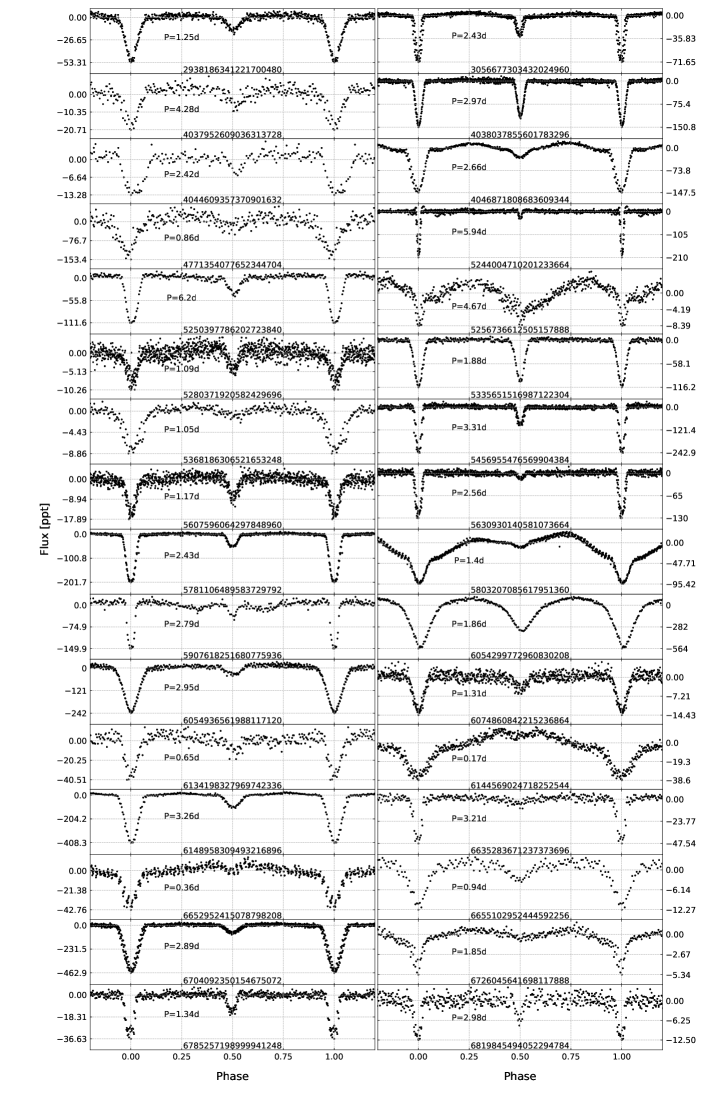
Figure 6: Phased time-series data of eclipsing binaries that show both primary and secondary eclipses and are likely detached or semi-detached binaries.

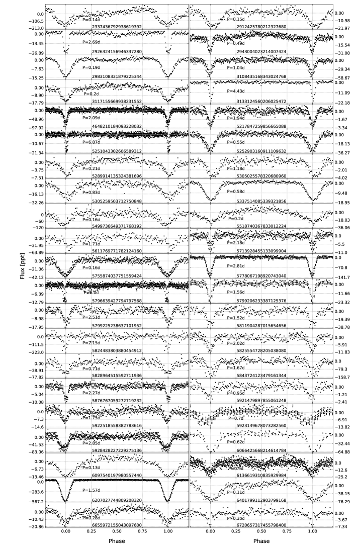
Figure 7: Phased time-series data of eclipsing binaries that show only primary eclipses.

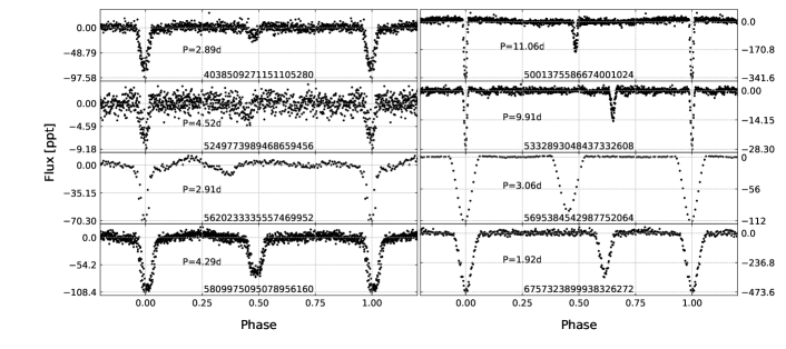
Figure 8: Phased/binned time-series data of eclipsing binaries with eccentric orbits.

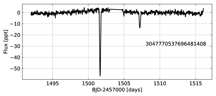
Figure 9: Time-series data of eclipsing binary Gaia DR2 3047770537696481408 with an eccentric orbit.

Table 3: Basic information of 32 eclipsing binaries that show both primary and secondary eclipses. We show the time-series data of these objects in Figure 6

Gaia DR2	TIC	G mag	Sector	Period[d]	Remarks
2938186341221700480	60523137	16.2325	6	1.2532	3 bright objects within 21"
3056677303432024960	753916356	17.9663	7	2.4282	3 objects within 21"
4037952609036313728	1556986400	18.8581	13	4.2844	very crowded field
4038037855601783296	1557298522	17.1815	13	2.9735	2 objects within 17"
4044609357370901632	1569961982	16.4584	13	2.415	very crowded field
4046871808683609344	1577179385	17.9382	13	2.6564	crowded field
4771354077652344704	685209944	17.0220	3-6,10,13	0.8619	-
5244004710201233664	371323868	16.7718	10,11	5.9367	2 bright objects within 30"
5250397786202723840	847157315	17.3345	9-11	6.1989	crowded field
5256736612505157888	462454783	13.0236	9-10	4.6739	-
5280371920582429696	176935277	15.8967	1-13	1.0922	-
5335651516987122304	321175529	12.1788	10-11	1.8844	crowded field
5368186306521653248	146317976	14.3942	9-10	1.0496	crowded field
5456955476569904384	942871718	18.0126	9	3.3063	very bright star 9" away
5607596064297848960	778203221	17.2286	7	1.1652	-
5630930140581073664	827970537	17.0919	8,9	2.5561	3 bright objects within 20"
5781106489583729792	309959661	16.1617	12-13	2.4251	2 bright objects within 20"
5803207085617951360	1509000006	16.6916	12-13	1.3974	object 14" away
5907618251680775936	1155805356	18.0498	11	2.7874	a bright star is at 12"
6054299772960830208	976146222	16.7204	10-11	1.8626	very crowded field
6054936561988117120	450420664	10.6360	11	2.9541	Avvakumova et al. (2013)
6074860842215236864	990883707	18.0659	11	1.3087	2 objects within 21"
6134198327969742336	996495522	17.9314	10-11	0.6491	-
6144569024718252544	258379678	15.3605	10	0.1739	Drake et al. (2017); HW Vir
6148958309493216896	998016645	18.0266	10	3.2584	3 bright objects within 21"
6635283671237373696	1689813971	18.9809	13	3.2146	2 bright objects within 21"
6652952415078798208	76760933	13.8504	13	0.3613	HW Vir candidate
6655102952444592256	1817787859	16.5162	13	0.9444	-
6704092350154675072	1692824895	16.7411	13	2.8881	CRTS J183755.6-484955 (Drake et al., 2017)
6726045641698117888	1701292115	9.1796	13	1.8459	3 objects nearby
6785257198999941248	270535918	13.4223	1	1.3423	-
6819845494052294784	2028782100	18.2564	1	2.9797	-

Table 4: Basic information of 42 eclipsing binaries that show primary eclipses only. We show the time-series data of these objects in Figure 7.

Gaia DR2	TIC	G mag	Sector	Period[d]	Remarks
2337436792938619392	33984762	15.4745	2	0.1445	Nova (Samus et al., 2017)
2912425780212327680	37737816	16.9636	6	0.1488	-
2926324156946337280	707111651	17.8191	6-7	2.6908	object 10" away
2943004023214007424	33743252	14.0155	6	0.4886	2 objects within 25"; HW Vir candidate
2983108331879225344	189012795	15.3166	5	0.1889	object 13" away
3108435168343024768	756875938	17.2058	7	1.0354	2 bright objects within 21"
3117155669938231552	42566802	16.0394	6	0.1986	HW Vir candidate
3133124560206025472	202273662	12.3871	6	4.4319	2 objects within 21"
4648210184093228032	141280240	15.7999	1-2,4-12	2.0908	-
5217847259856665088	843283217	17.9546	10-12	1.9444	object 16" away
5251043302606589312	847473488	18.2467	9-10	6.8704	3 objects within 21"
5252903160911109632	849266771	18.8591	10-11	0.5458	crowded field
5289914135324381696	308541002	16.5557	1,4,7-11	0.2105	HW Vir candidate
5305025578320680960	383375636	15.5078	8-10	1.1821	crowded field
5305259503712750848	856066667	18.4776	9	0.8298	4 bright objects within 21"
5337514085339321856	280246753	12.2093	10-11	0.5821	crowded field
5499736649371768192	255594396	17.4141	1-2,5-9,11-12	0.1585	-
5518740367833012224	818308005	17.4758	7-8,9	0.2049	2 bright objects within 21"
5611769771782124160	779128665	18.9927	7	1.7065	4 brighter objects within 21"
5713928455133099904	834924649	18.3591	7	2.1812	2 objects within 21"
5755874037751559424	95785714	15.8131	8	0.1559	-
5778067198920743040	1309769412	17.8042	12-13	2.8099	object 5" away
5796639427794797568	401617089	13.1231	12	5.9992	3 objects within 26"
5799206233387125376	1106932458	18.1909	12	1.5615	crowded field
5799225238637101952	1106947173	18.2872	12	2.5142	-
5811904287015654656	1509561926	17.7235	12-13	1.5239	2 objects within 21"
5824483803880454912	1110889969	17.7445	12	2.1506	crowded field
5825554728205038080	424717152	15.0860	12	2.0156	bright object 9" away
5828964515592711936	1209068896	17.3298	12	0.7066	5 objects within 21"
5843724123479161344	957158511	17.2414	11-12	1.673	crowded field
5876767059272719232	1130777039	15.8884	12	2.2711	crowded field
5921479897855061248	1513749999	18.3774	12	0.9524	crowded field
5922518558382783616	1315988153	18.8932	12	1.7541	3 bright objects within 21"
5923149678073282560	1316233834	18.4008	12	0.698	3 bright objects within 21"
5928428227229275136	1219774587	18.9003	12	2.8496	crowded field
6066425668214614784	986927321	17.3006	11	0.6241	very crowded field
6097540197980557440	242402846	16.3590	11	0.1274	-
6136619310835929984	996840740	18.3096	11	0.9006	object 14" away
6207027744809208320	1174994870	17.7766	11	1.5731	-
6401799112903799168	410442849	14.6995	13	0.1117	CV (O’Donoghue et al., 2013)
6655972155043097600	456516418	13.5608	13	0.2786	-
6720657317455798400	1695999069	16.2634	13	0.3536	crowded field

Table 5: Basic information of nine eclipsing binaries with eccentric orbits. We show the time-series data of these objects in Figures 8 and 9

Gaia DR2	TIC	G mag	Sector	Period[d]	Remarks
3047770537696481408	187657618	9.8610	7	-	TYC 5395-2586-2 nearby
4038509271151105280	1558593400	18.7875	13	2.8936	very crowded field
5001375586674001024	616535392	18.7768	2	11.0648	-
5249773989468659456	846855557	18.4170	9-11	4.5177	2 objects within 21"
5332893048437332608	305898260	11.8255	10-11	9.9141	crowded field
5620233335557469952	139334900	13.0033	7	2.9054	-
5695384542987752064	832426099	9.8621	8	3.0607	AC Pyx (Samus et al., 2003)
5809975095078956160	1509255862	18.9775	12-13	4.2926	2 bright objects within 21"
6757323899938326272	1826847776	18.8560	13	1.9224	3 bright objects within 21"

3.4 Spectroscopically unclassified variables

We found a spectroscopically unidentified sample of 1536 variable stars that we identified neither as pulsators nor as eclipsing binary systems, presented in the previous subsections. The proper variability type can only be done with a spectroscopic classification and radial velocity curves. We split this sample into two groups.

The first group contains targets that show peaks consistent with binarity, and amplitudes of a flux variation that is large enough to be clearly seen in phased data. The typical S/N is 45. The phased time-series data of these objects show either one maximum or two maxima of a flux variation. Those with one maximum can be symmetric or asymmetric. The symmetric case can be interpreted as a reflection binary (Baran et al., 2019). The asymmetric case is characteristic of some of the classical pulsators, e.g. RR Lyrae stars, anomalous Cepheids, classical Cepheids. Two maxima cases can be explained by ellipsoidal variables or contact eclipsing binaries e.g. W UMa stars. If the maxima are not equal, it may indicate a Doppler boosting contribution (former case), which can even end up with just one maximum mimicking a reflection binary (Reed et al., 2016), or the O’Connell effect (latter case). Examples of all these three cases selected in our sample are plotted in Figure 10. We provided basic information about these targets in Table 6, while the data are plotted in Figure 10.

The second group contains targets that show peaks consistent with binarity, and flux variation amplitudes that are too small to be clearly seen in phased data. The typical S/N is 8. We find these variations in amplitude spectra. This group contains also targets with multipeak amplitude spectra, regardless of the S/N, which makes data phasing unnecessary. This multiplicity of peaks is characteristic of pulsators, however the amplitude spectra do not resemble the ones of sdBVs, since the unrelated peaks are below 60 $\upmu$Hz, and that is why we decided not to include them in Section 3.2. We found flux variations in targets of this group in their amplitude spectra. We provided basic information about these targets in Table 7, while the data are plotted in Figure 11.

We have also detected two Nova stars, Gaia DR2 5207384891323130368 and Gaia DR2 6544371342567818496, during outbursts. The latter star is spectroscopically classified and formally included in the subsequent subsection. We show the time-series data in Figure 12. Both stars have been known before but TESS data recorded outbursts and that is why we included these objects in our list. More information on these two objects can be find in Table 8. Other known Nova detected in our sample are not specifically mentioned, since time-series data of these objects do not show significant outbursts.

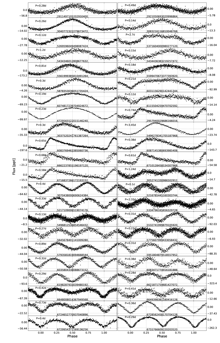
Figure 10: Phased time-series data for variable objects that are spectroscopically unclassified. The first fifteen objects have one symmetric maximum, the next eight objects have one asymmetric maximum, and the final twenty-one objects have two maxima.

Figure 11: Amplitude spectra of variable objects that are spectroscopically unclassified.

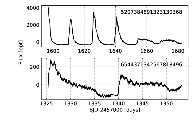
Figure 12: Time-series data during outbursting of two Nova stars.

Table 6: Basic information of 44 (out of 273) spectroscopically unclassified variables. The top section lists 15 objects that show one symmetric maximum, the middle section lists eight objects that show one asymmetric maximum, and the bottom section lists 21 objects that show two maxima. We show phased time-series data of these objects in Figure 10. The list of remaining objects (229) are included in on-line material only.

Gaia DR2	TIC	G mag	Sector	Period[d]	Remarks
2911497105202950400	37004041	15.1572	6	0.2833	Drake et al. (2017)
2921050693020996864	63113578	11.4451	6-7	0.4854	object 11" away
3040772322279673472	32302937	14.2637	7	0.2618	-
3083216116810048768	73238638	15.3182	7	0.1376	-
5269596049498087424	765017261	17.1323	1-13	0.1247	-
5371604000980277120	61762775	12.6910	10	2.7027	-
5434346012808677632	70717873	13.6554	9	1.2048	-
5434436383219257472	29723252	14.0488	9	0.1502	-
5561999385810491264	170310610	15.3198	6-7	0.813	Drake et al. (2017)
5599470673377393920	775878600	16.1312	7	0.1767	-
5878353036051735424	1036707862	15.0629	11-12	0.3026	crowded field
6031156290142441344	191221080	12.8298	12	0.2053	crowded field
6074817239704924672	990861367	17.7796	11	0.1887	-
6115504259470702592	166894438	15.8446	11	0.1238	-
6729565522015146240	1821904001	18.1963	13	0.2268	TYC 7919-615-1 20" away
2957940029686166016	708350292	17.5007	5-6	0.7353	very crowded field
3037520241761387264	750862698	18.9978	7	0.3003	5 objects within 21"
5496278341705187968	737473774	16.7776	1-13	3.4483	bright object 13" away
6083769463385060736	1048223010	16.7149	11	0.6536	-
6087145380693985408	1048399825	18.8821	11	0.3831	-
6662237855196197120	1818520053	18.8787	13	0.6849	2 objects within 21"
6710128458534307968	1819242966	18.3171	13	0.6098	4 objects within 21"
6716837266172193152	1820684543	18.5151	13	0.578	3 objects within 21"
3052741330986502912	125197892	12.7196	7	1.2426	3 objects within 25"
3070438000690624384	803473779	17.6109	7	0.4016	3 objects within 21"
5216785445160303744	287977499	12.5806	6,10-12	0.0976	Ratzloff et al. (2019)
5217109006519074176	804970406	18.7363	10-12	0.3344	3 objects within 21"
5334796165656329728	325158549	11.0515	10-11	2.3256	crowded field
5496812536854546432	278861557	15.2643	1-13	0.1318	Kosakowski et al. (2020)
5532741999879105920	821330826	17.5457	7-8	0.3077	3 objects within 21"
5645678401141009280	830270910	18.8839	8	0.2713	2 bright objects within 21"
5775607999433058432	1205184125	16.7156	12-13	0.2342	-
5793581819094668544	1105179202	18.9163	12	0.8929	2 bright objects within 21"
5951804879518557952	1523243111	17.5232	12	0.3058	very crowded field
6035804338088673152	1255310693	18.8790	12	0.3185	4 bright objects within 21"
6083471774916181888	1048022421	17.0149	11	0.3774	2 bright objects within 21"
6198287933039480192	1173764699	17.0215	11	0.2857	-
6621871759681427072	2028297898	18.8353	1	0.2833	-
6648008014367949568	1690227091	17.0039	13	0.4157	-
6649398381180416128	119153557	16.3566	13	0.4132	object 7" away
6724652770937040896	1699111897	17.1528	13	0.7317	crowded field
6728562458170704128	1821458807	17.1410	13	0.3584	bright object 8" away
6729954371169136256	1704724045	18.6622	13	0.3953	crowded field
6755766609220203520	1826089601	17.7117	13	0.2933	2 objects within 21"

Table 7: Basic information of 26 (out of 1262) spectroscopically unclassified variables. We show amplitude spectra of these objects in Figure 11. The figures of remaining objects (1236) are included in on-line material only.

Gaia DR2	TIC	G mag	Sector	Remarks
2494281851762928512	250416977	14.3723	4	Nova (Downes et al., 2001)
2922496653888398976	744429291	10.7118	6-7	TYC 6522-1975-1 2" away
4035494852634865664	1552304995	16.7775	13	crowded field
4044733572133754240	1570330815	18.6726	13	very crowded field
5255832397304667264	852628533	17.7834	9-11	-
5263888695091870976	271554913	15.9580	1-7,9-13	-
5313049268735645312	299705972	16.2419	9-10	-
5332775190225061504	321662350	15.4428	10-11	2 bright objects within 15"
5407274838253246720	867297951	17.8164	9-10	crowded field
5416786571595520768	870414976	17.5691	9	3 objects within 21"
5594391097148387712	151005205	16.8940	7-8	TYC 7123-1718-1 19" away
5596751409325049856	154909544	15.0666	7-8	2 objects within 21"
5610727198536681600	778822592	16.0649	6-7	object 17" away
5611674977567099648	109931573	15.9019	7	crowded field
5758065776742268544	60659496	15.3353	8	-
5817603850371030528	447448883	15.6791	12	5 bright objects within 21"
5850711622986006272	1012682181	16.2865	11-12	crowded field
5852787840208469760	1017631564	16.3352	11-12	crowded field
5875446992500886784	455460222	10.7497	12	-
5886385827467871488	46197886	16.0325	12	4 objects within 21"
5954096772853080448	1526877224	17.4808	13	2 objects within 21"
6083675803027407872	1048099460	16.8865	11	very crowded field
6707713694774167424	1694125610	16.6361	13	object 13" away
6721011463293001216	1696341981	18.5560	13	crowded field
6727998894039826304	1703871394	18.4060	13	very crowded field
6728063696533517696	1703965520	18.9681	13	crowded field

3.5 Non-sdB classified variables

We have also pulled out fluxes of additional 77 objects that are spectroscopically classified. These were first considered candidates for hot stars, but spectral analyses confirmed them as non-sdB objects, mostly O, B or A main sequence stars. We found the same collection of a flux variation as in case of the sample of spectroscopically unclassified objects and we present it grouped the same way, i.e. pulsator candidates, eclipsing, reflection, ellipsoidal binaries, and classical pulsators. A table and figures showing the list of objects with their data are included in the on-line material only. The table includes basic information on each object along with additional references or contaminating objects, if any. The spectroscopically classified nova showing outbursts is included in Table 8.

Table 8: Basic information of two Nova stars. We show the time-series data in Figure 12. Both stars are reported by Samus et al. (2003).

Gaia DR2	TIC	Name	Spectral type	G mag	Sector
5207384891323130368	735128403	AH Men	-	13.5101	1,4,11-13
6544371342567818496	121422158	RZ Gru	B6	12.6299	1

4 Mode identification

We selected five objects out of 83 non-classified pulsators to identify their pulsation geometry by assuming them as g-mode rich sdBVs. Gaia DR2 IDs of these objects are 5233348350879239680, 5250674622612902912, 5365175740610237568, 5391470732981138816, 6096794282417069696. We provided arguments for our selection in Section 3.2.

We followed a standard prewhitening procedure by calculating an amplitude spectrum and removing consecutive peaks by fitting $A_{i}\sin(2{\pi}f_{i}t+{\phi_{i}})$ using a non-linear least-square method, where A_i is an amplitude, f_i is a frequency and $\phi_{i}$ is a phase of an i-th peak. We used our custom scripts for prewhitening. We removed all peaks down to a detection threshold of 4.5 times the mean noise level. We updated this level after each peak removal, hence the final level was calculated from the residual amplitude spectra, i.e. with all significant peaks removed. The lists of frequencies detected in each star are listed in Tables 9, 10, 11, 12 and 13, while we show the amplitude spectra in Figure 13.

In the case of no rotation, one cannot tell the non-radial modes of degree (l) value of a peak, as only one peak is present. Rotation splits a mode into 2l+1 components of different m values. The frequency shift is given by the following equation $\Delta{\nu}_{n,l,m}=1-C_{n,l}/P_{\rm rot}$. According to Charpinet et al. (2000), for gravity modes, the Ledoux constant C_n,l, can be calculated from the following expression $C_{n,l}=(l^{2}+1)^{-1}$. When the frequency shift is measured in an amplitude spectrum, a rotation period P_rot can be derived. The formulas for the frequency shift and for $C_{n,l}$ assume first order corrections and are in the asymptotic limits since the frequency range corresponds to an overtone number of 20 or greater in a typical sdBV star.

In sdBVs, in the asymptotic regime i.e. $n\gg l$, consecutive overtones of gravity modes are equally spaced in period (e.g. Charpinet et al., 2000; Reed et al., 2011). Previous analyses of photometric Kepler space data of sdBVs showed that the average period spacing of dipole modes is nearly 250 s (Reed et al., 2018). The period spacings for higher degree modes can be calculated using the following relation $\Delta P_{l}={P_{0}}/{\sqrt{l(l+1)}}$.

We searched for multiplet candidates and we only found a few examples of split dipole modes in Gaia DR2 5233348350879239680. We marked these peaks with ’*’ in Figure 13. In Table 9 we added an azimuthal order assignment according to the splitting. If a single splitting is measured, f₂, f₃ and f₄, f₅ we arbitrarily chose one of the peaks to be the central (m = 0) component. In case of f₁₂, f₁₃, the splitting is doubled so we may have detected only the side components. Assuming our multiplet identification is correct the average rotation period equals 5.238(48) days. The non-split modes are arbitrarily chosen to central components m = 0.

The multiplet detection helps to constrain the modal degree and provides a head start for determining the asymptotic period spacing, as these three pairs of peaks were assigned l = 1 modes. In all other cases, including four other stars, we found no additional hints of a modal degree preference and we decided to assign l = 1 to any peaks that are spaced by a period spacing between 200 and 300 sec. Those peaks not satisfying our requirements were assigned either l = 2 or a trapped l = 1 mode. The latter happened only in Gaia DR2 5391470732981138816. The average period spacings of dipole modes we measured in these stars are 288.20 (1.08) s (Gaia DR2 5233348350879239680), 279.50 (35) s (Gaia DR2 5250674622612902912), 274.30 (1.26) s (Gaia DR2 5365175740610237568), 267.84 (78) s (Gaia DR2 5391470732981138816), 248.74 (1.29) s (Gaia DR2 6096794282417069696). We included the resultant radial order and modal degree assignment in Tables 9 – 13.

Table 9: List of frequencies detected in Gaia DR2 5233348350879239680.

ID	Frequency	Period	Amplitude	S/N	l	m	n
	[$\upmu$Hz]	[s]	[ppt]
f1	76.667(8)	13043.4(1.4)	0.824(57)	12.5	1	0	46
f2	85.977(11)	11631.1(1.5)	0.575(57)	8.7	1	0	41
f3	87.073(9)	11484.6(1.2)	0.716(57)	10.8	1	-1	41
f4	90.534(6)	11045.5(7)	1.143(57)	17.3	1	0	39
f5	91.653(12)	10910.7(1.5)	0.529(57)	8.0	1	-1	39
f6	99.142(11)	10086.5(1.1)	0.585(57)	8.9	2	0	62
f7	101.635(11)	9839.1(1.1)	0.572(57)	8.7	1	0	35
f8	104.81(2)	9541.2(1.8)	0.331(57)	5.0	1	0	34
f9	107.499(9)	9302.4(8)	0.714(57)	10.8	1	0	33
f10	141.584(3)	7063.0(2)	2.096(57)	31.7	1	0	25
f11	142.361(19)	7024.4(9)	0.35(57)	5.3	-	-	-
f12	147.615(9)	6774.40(42)	0.718(57)	10.9	1	+1	24
f13	149.814(9)	6674.94(40)	0.728(57)	11.0	1	-1	24
f14	171.236(3)	5839.9(1)	2.522(57)	38.2	1	0	21
f15	177.34(2)	5638.8(6)	0.324(57)	4.9	2	0	35
f16	183.17(1)	5459.57(30)	0.646(57)	9.8	2	0	34
f17	190.303(13)	5254.79(35)	0.518(57)	7.8	1	0	19
f18	219.98(2)	4545.97(41)	0.334(57)	5.1	-	-	-
f19	228.411(25)	4378.08(48)	0.261(57)	4.0	1	0	16

Table 10: List of frequencies detected in Gaia DR2 5250674622612902912.

ID	Frequency	Period	Amplitude	S/N	l	n
	[$\upmu$Hz]	[s]	[ppt]
f1	41.327(16)	24197(10)	0.224(47)	4.7	1	87
f2	47.94(11)	20859.4(4.9)	0.325(47)	6.9	1	75
f3	64.508(15)	15501.9(3.7)	0.24(5)	5.1	1	56
f4	82.56(1)	12112.1(1.4)	0.384(47)	8.2	2	75
f5	103.236(5)	9686.5(5)	0.706(47)	15.0	1	35
f6	109.111(12)	9165.0(1.0)	0.306(47)	6.4	2	57
f7	125.473(3)	7969.9(2)	1.28(5)	27.1	1	29
f8	145.12(1)	6890.8(5)	0.36(5)	7.6	1	25
f9	152.038(17)	6577.3(7)	0.215(47)	4.6	1	24
f10	166.346(13)	6011.6(5)	0.28(5)	5.9	-	-
f11	166.56(1)	6003.7(4)	0.356(47)	7.5	-	-
f12	166.766(2)	5996.4(1)	1.913(47)	40.6	1	22
f13	166.982(8)	5988.6(5)	0.466(47)	9.9	-	-
f14	214.713(13)	4657.4(3)	0.278(47)	5.9	1	17

Table 11: List of frequencies detected in Gaia DR2 5365175740610237568.

ID	Frequency	Period	Amplitude	S/N	l	n
	[$\upmu$Hz]	[s]	[ppt]
f1	84.074(13)	11894.3(1.8)	0.412(42)	8.4	1	44
f2	99.793(18)	10020.7(1.8)	0.291(42)	5.9	1	37
f3	101.038(23)	9897.3(2.3)	0.228(42)	4.6	-	-
f4	112.816(4)	8864.02(33)	1.238(42)	25.1	1	33
f5	128.048(14)	7809.6(9)	0.377(42)	7.7	1	29
f6	132.607(15)	7541.1(9)	0.349(42)	7.1	1	28
f7	136.978(14)	7300.4(8)	0.371(42)	7.5	1	27
f8	143.537(19)	6966.9(9)	0.276(42)	5.6	1	26
f9	168.952(3)	5918.85(9)	2.053(42)	41.6	1	22
f10	173.128(24)	5776.1(8)	0.219(42)	4.4	-	-
f11	175.858(2)	5686.40(7)	2.457(42)	49.8	2	36
f12	177.531(29)	5632.8(9)	0.181(42)	3.7	-	-
f13	177.668(2)	5628.48(6)	2.768(42)	56.1	1	21
f14	193.201(7)	5175.94(19)	0.726(42)	14.7	2	33
f15	196.89(1)	5078.75(26)	0.527(42)	10.7	-	-
f16	198.388(7)	5040.64(17)	0.807(42)	16.4	1	19
f17	202.604(25)	4935.7(6)	0.213(42)	4.3	-	-
f18	224.079(22)	4462.71(43)	0.243(42)	4.9	1	17

Table 12: List of frequencies detected in Gaia DR2 5391470732981138816.

ID	Frequency	Period	Amplitude	S/N	l	n
	[$\upmu$Hz]	[s]	[ppt]
f1	66.562(19)	15023.6(4.2)	0.65(1)	5.4	1	57
f2	81.086(11)	12332.6(1.6)	1.12(1)	9.3	1	47
f3	88.754(21)	11267.1(2.7)	0.57(1)	4.7	1	43
f4	97.621(15)	10243.7(1.6)	0.82(1)	6.8	1	39
f5	103.09(12)	9700.3(1.2)	0.99(1)	8.2	1	37
f6	105.592(22)	9470.5(2.0)	0.54(1)	4.5	-	-
f7	106.448(19)	9394.2(1.7)	0.64(1)	5.3	1	36
f8	121.176(21)	8252.5(1.4)	0.59(1)	4.9	2	54
f9	131.49(2)	7605.4(1.1)	0.62(1)	5.1	2	50
f10	140.108(18)	7137.4(9)	0.67(1)	5.5	2	47
f11	141.623(17)	7061.0(8)	0.72(1)	5.9	1	t
f12	143.025(22)	6991.8(1.1)	0.54(1)	4.5	1	27
f13	169.373(12)	5904.14(42)	1.02(1)	8.4	1	23

Table 13: List of frequencies detected in Gaia DR2 6096794282417069696.

ID	Frequency	Period	Amplitude	S/N	l	n
	[$\upmu$Hz]	[s]	[ppt]
f1	98.741(18)	10127.5(1.8)	1.582(92)	15.2	1	41
f2	138.863(19)	7201.3(1.0)	1.535(92)	14.7	1	29
f3	148.208(47)	6747.3(2.1)	0.607(92)	5.8	2	46
f4	161.876(11)	6177.57(43)	2.496(92)	23.9	1	25
f5	235.547(24)	4245.44(43)	1.201(92)	11.5	2	29
f6	239.563(36)	4174.3(6)	0.786(92)	7.5	1	17
f7	272.763(49)	3666.2(7)	0.578(92)	5.5	1	15

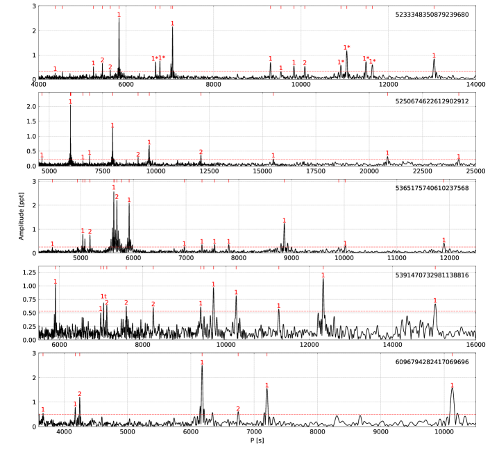
Figure 13: Amplitude spectra of five pulsators plotted versus period (instead of frequency). The red horizontal dashed lines denote $4.5\,\sigma$ detection threshold. The values of modal degrees are shown on top of each detected peak.

5 Summary

To date, the sample of sdBVs has been selected by random discoveries made from ground-based and space observations. This limits the study of sdBVs to individual cases only and it does not allow for inferring how pulsation properties depend on a stellar population. We undertook a search for sdBVs candidates selected from a sdB database Geier (2020) and based on an all-sky photometry collected during the TESS mission in the LC mode. This data still limits our search to g-mode sdBVs, which is a consequence of a 30 min. cadence, however the search utilizes the most updated sdB database along with the only all-sky space survey, allowing for the most complete sample of g-mode sdBVs currently possible.

Many sdBV candidates are allocated for TESS SC monitoring and these objects have time-series data pulled out and ready for variability check. We focused on additional sample of sdBV candidates that are located on TESS silicons but with no automated time-series data pulled out. We have prepared and used a set of applications and scripts that allowed us to derive the fluxes and to calculate amplitude spectra to detect a significant flux variation.

From time-series data and amplitude spectra, we detected significant variability in 1807 (out of 20,642) objects. 28 objects are classified as sdBs and only two of them show convincing pulsations. One object shows eclipses and a reflection effect typical of HW Vir systems, while the remaining 25 sdBs show significant signal in their amplitude spectra, which we interpreted as a binary signature. A sample of 77 objects not classified as sdBs were found to be variable and we include them in this paper (on-line material) for completeness and as a resource for others. The remaining 1702 objects were found to be variable but are spectroscopically unclassified, hence we are unable to verify if they are sdBVs or another type of variable stars yet. In this group we found 83 objects showing a significant signal typical of g-modes in sdBVs. We selected the five objects best-suited for mode identification and assigned modal degrees. We used multiplets and a period spacing for this purpose. The sequences of presumably same degree overtones are not too complete but the multiples of 250 sec (ish) can still be found. This may be another argument for these objects being sdB stars. However, our identification will only be reliable if these objects are spectroscopically confirmed to be sdBs. Regardless the correctness of our choice, other objects are not suitable for the mode identification since the signal we detected either has too few peaks or the peaks are too close to the Nyquist frequency.

We also found 83 eclipsing binaries and organized them into three subgroups based on their eclipse content. We found 32 objects that show both primary and secondary eclipses, 42 objects that show only primary eclipses, and nine objects that show secondary eclipses out of 0.5 phase, indication of eccentric orbits. The last sample of variables contains 1535 objects that show either binary signatures or classical pulsator asymmetric light curves. 273 objects show flux variation amplitudes that are large enough to see in phased time-series data. These objects show one symmetric maximum, one asymmetric maximum, and two maxima. The remaining 1262 objects show amplitude spectra that are consistent with binarity.

We also detected flux variations in two known novae, of which only one is spectroscopically classified.

Our search for variable sdB stars in TESS LC data reveals a few new and more than a thousand candidates for sdBVs. We used our discoveries to propose those candidates to be observed in either 2 min or 20 sec cadence, during the second run of TESS in the southern ecliptic hemisphere. If these objects are allocated the upcoming data may bring additional discoveries of p-modes, confirming their sdB nature. Our work is the first focused on an all-sky TESS survey to search for sdBVs and, when the spectral classification is performed, we consider it to be the most updated list of sdBVs in the southern ecliptic hemisphere. Such a sample will be very useful to understand the pulsation–population relationship.

Data availability

The datasets were derived from MAST in the public domain archive.stsci.edu.

References

- Avvakumova et al. (2013) Avvakumova E. A., Malkov O. Y., Kniazev A. Y., 2013, Astronomische Nachrichten, 334, 860
- Baran et al. (2005) Baran A., Pigulski A., Kozieł D., Ogłoza W., Silvotti R., Zoła S., 2005, MNRAS, 360, 737
- Baran et al. (2015) Baran A. S., Koen C., Pokrzywka B., 2015, MNRAS, 448, 16
- Baran et al. (2018) Baran A. S., et al., 2018, Monthly Notices of the Royal Astronomical Society, 481, 2721
- Baran et al. (2019) Baran A., Telting J., Jeffery C., Østensen R., Vos J., Reed M., Vučković M., 2019, MNRAS, 489, 1556
- Bonnarel, F. et al. (2000) Bonnarel, F. et al., 2000, Astron. Astrophys. Suppl. Ser., 143, 33
- Borucki et al. (2010) Borucki W. J., et al., 2010, Science, 327, 977
- Boudreaux et al. (2017) Boudreaux T. M., et al., 2017, The Astrophysical Journal, 845, 171
- Brasseur et al. (2019) Brasseur C. E., Phillip C., Fleming S. W., Mullally S. E., White R. L., 2019, Astrocut: Tools for creating cutouts of TESS images (ascl:1905.007)
- Brown et al. (1997) Brown T. M., Ferguson H. C., Davidsen A. F., Dorman B., 1997, ApJ, 482, 685
- Charpinet et al. (1997) Charpinet S., Fontaine G., Brassard P., Chayer P., Rogers F. J., Iglesias C. A., Dorman B., 1997, ApJ, 483, 123
- Charpinet et al. (2000) Charpinet S., Fontaine G., Brassard P., Dorman B., 2000, ApJS, 131, 223
- Downes et al. (2001) Downes R. A., Webbink R. F., Shara M. M., Ritter H., Kolb U., Duerbeck H. W., 2001, PASP, 113, 764
- Drake et al. (2017) Drake A. J., et al., 2017, Monthly Notices of the Royal Astronomical Society, 469, 3688
- Feinstein et al. (2019) Feinstein A. D., et al., 2019, Publications of the Astronomical Society of the Pacific, 131, 094502
- Fontaine et al. (2003) Fontaine G., Brassard P., Charpinet S., Green E., Chayer P., Billères M., Randall S., 2003, ApJ, 597, 518
- Gaia Collaboration (2018) Gaia Collaboration 2018, A&A, 616, A10
- Geier (2020) Geier S., 2020, A&A, 635, A193
- Geier et al. (2019) Geier S., Raddi R., Gentile Fusillo N., Marsh T., 2019, A&A, 621, A38
- Heber (2016) Heber U., 2016, PASP, 128, 2001
- Høg et al. (2000) Høg E., et al., 2000, A&A, 355, L27
- Holdsworth et al. (2017) Holdsworth D. L., Østensen R. H., Smalley B., Telting J. H., 2017, Monthly Notices of the Royal Astronomical Society, 466, 5020
- Kilkenny et al. (1997) Kilkenny D., Koen C., O’Donoghue D., Stobie R. S., 1997, Monthly Notices of the Royal Astronomical Society, 285, 640
- Kosakowski et al. (2020) Kosakowski A., Kilic M., Brown W. R., Gianninas A., 2020, The Astrophysical Journal, 894, 53
- Kupfer, T. et al. (2015) Kupfer, T. et al., 2015, A&A, 576, A44
- Kupfer et al. (2017) Kupfer T., et al., 2017, The Astrophysical Journal, 835, 131
- Lei et al. (2018) Lei Z., Zhao J., Németh P., Zhao G., 2018, The Astrophysical Journal, 868, 70
- Lei et al. (2019a) Lei Z., Bu Y., Zhao J., Németh P., Zhao G., 2019a, Publications of the Astronomical Society of Japan, 71
- Lei et al. (2019b) Lei Z., Zhao J., Németh P., Zhao G., 2019b, The Astrophysical Journal, 881, 135
- Lightkurve Collaboration et al. (2018) Lightkurve Collaboration et al., 2018, Lightkurve: Kepler and TESS time series analysis in Python, Astrophysics Source Code Library (ascl:1812.013)
- Luo et al. (2019) Luo Y., Németh P., Deng L., Han Z., 2019, The Astrophysical Journal, 881, 7
- O’Donoghue et al. (2013) O’Donoghue D., Kilkenny D., Koen C., Hambly N., MacGillivray H., Stobie R. S., 2013, MNRAS, 431, 240
- Pretorius & Knigge (2008) Pretorius M. L., Knigge C., 2008, MNRAS, 385, 1471
- Randall et al. (2009) Randall S., van Grootel V., Fontaine G., Charpinet S., Brassard P., 2009, A&A, 507, 911
- Ratzloff et al. (2019) Ratzloff J. K., et al., 2019, The Astrophysical Journal, 883, 51
- Ratzloff et al. (2020) Ratzloff J. K., et al., 2020, The Astrophysical Journal, 890, 126
- Reed et al. (2011) Reed M. D., et al., 2011, MNRAS, 414, 2885
- Reed et al. (2012) Reed M. D., Baran A., Østensen R. H., Telting J. H., O’Toole S. J., 2012, MNRAS, 427, 1245
- Reed et al. (2016) Reed M. D., et al., 2016, MNRAS, 458, 1417
- Reed et al. (2018) Reed M., et al., 2018, Open Astronomy, 27, 157
- Ricker et al. (2014) Ricker G. R., et al., 2014, Transiting Exoplanet Survey Satellite (TESS), doi:10.1117/12.2063489
- Samus et al. (2003) Samus N. N., et al., 2003, Astronomy Letters, 29, 468
- Samus et al. (2017) Samus N. N., Kazarovets E. V., Durlevich O. V., Kireeva N. N., Pastukhova E. N., 2017, Astronomy Reports, 61, 80
- Taylor (2005) Taylor M. B., 2005, TOPCAT & STIL: Starlink Table/VOTable Processing Software. p. 29
- Vos et al. (2018) Vos J., Vučković M., Chen X., Han Z., Boudreaux T., Barlow B. N., Østensen R., Németh P., 2018, Monthly Notices of the Royal Astronomical Society, 482, 4592
- Wenger, M. et al. (2000) Wenger, M. et al., 2000, Astron. Astrophys. Suppl. Ser., 143, 9
- Wood et al. (1993) Wood J. H., Zhang E.-H., Robinson E. L., 1993, Monthly Notices of the Royal Astronomical Society, 261, 103
- de Boer (1985) de Boer K., 1985, A&A, 142, 321