Improving Sales Forecasting Accuracy: A Tensor Factorization Approach with Demand Awareness

Abstract

Due to accessible big data collections from consumers, products, and stores, advanced sales forecasting capabilities have drawn great attention from many companies especially in the retail business because of its importance in decision making. Improvement of the forecasting accuracy, even by a small percentage, may have a substantial impact on companies’ production and financial planning, marketing strategies, inventory controls, supply chain management, and eventually stock prices. Specifically, our research goal is to forecast the sales of each product in each store in the near future. Motivated by tensor factorization methodologies for personalized context-aware recommender systems, we propose a novel approach called the Advanced Temporal Latent-factor Approach to Sales forecasting (ATLAS), which achieves accurate and individualized prediction for sales by building a single tensor-factorization model across multiple stores and products. Our contribution is a combination of: tensor framework (to leverage information across stores and products), a new regularization function (to incorporate demand dynamics), and extrapolation of tensor into future time periods using state-of-the-art statistical (seasonal auto-regressive integrated moving-average models) and machine-learning (recurrent neural networks) models. The advantages of ATLAS are demonstrated on eight product category datasets collected by the Information Resource, Inc., where a total of 165 million weekly sales transactions from more than 1,500 grocery stores over 15,560 products are analyzed.

Keywords: design science, machine learning, sales forecasting, tensor decomposition, consumer demand

1 Introduction

Supply chain and inventory management involve many complex problems, where decision makers (e.g., producers, distributors, store managers) typically need to consider a wide variety of aspects, including costs, inventory levels, transportation, labor, supply and demand trends, potential risks and gains. Product sales forecasting is a key component in many decision processes, and making accurate sales forecasts constitutes an important and challenging problem. For example, store managers often have to decide on the optimal inventory levels of products by making trade-offs between continuously re-stocking existing items and testing out alternative products to increase novelty, diversity, and serendipity. Effective forecasting techniques are needed, especially when there is little or no direct historical sales data for a specific product in a specific store.

One possible solution is to leverage sales data from similar stores and/or from similar products. Store managers could potentially acquire historical data of other stores from market research or consulting companies. Based on the trend and seasonality of product sales in other stores, a store manager could more accurately predict the future sales of a product in her store. Inspired by recommender systems (e.g., Aggarwal,, 2016), when there are rich data about product sales from other stores, one could consider employing collaborative filtering techniques (Breese et al.,, 1998; Su and Khoshgoftaar,, 2009; Walter et al.,, 2012; Lee and Hosanagar,, 2019) to take advantage of such information. The value of a collaborative recommender system for consumers is that it helps them deal with the information overload (Jacoby,, 1984; Horrigan,, 2016). In other words, it removes unwanted, irrelevant information and finds matched, personalized products in an efficient manner (Chen and Xie,, 2005; Liebman et al.,, 2019), thus, adding significant value to user experience and increasing product sales (Hosanagar et al.,, 2014). In the sales forecasting context, similarly, if collaborative filtering is incorporated properly, store managers could use it to filter out unpopular or non-profitable products and hence identify potentially profitable products from a great number of alternative choices.

However, the context of sales forecasting is different from recommender systems, and hence off-the-shelf collaborative filtering methods may not be directly applicable or effective. One major difference is that forecasting targets on predicting future values, whereas most preference-based recommendations aim at predicting users’ preferences over their unexperienced items, although time can still be taken into account as an important factor for quantifying dynamic user preferences (e.g., Koren et al.,, 2009; Koren, 2010a, ; Sahoo et al., 2012b, ; Aggarwal,, 2016). Another major difference is that product sales are also subject to the dynamics of consumer demand. For example, if one customer bought a TV from Target, s/he probably would not buy it again from Walmart within a short period of time. In contrast, for preference-based recommendation, for instance, one user could have high preferences for (and hence assign high ratings to) many movies. That is, in addition to the collaborative nature, sales forecasting also entails a competitive nature, where increased sales in one store may satisfy a large portion of local consumer demand, and hence result in reduced sales of similar products in other local stores.

Our work follows the design science paradigm (Hevner et al.,, 2004) in that it designs a data-driven, machine-learning methodology to improve forecasting accuracy for product sales. The problem setting consists of product sales at the store level, that is, weekly (or daily, monthly, etc.) transactions from $n$ brick-and-mortar grocery stores of $m$ products over weeks $1,2,\ldots,T$. For example, a sample data point could be “store #1 sold 80.95 dollars of beer #246 in week #3”. In this paper, our goal is to forecast the future sales of every product in every store in weeks $T+1$, $T+2$, etc.

The key contribution of this design artifact is that we incorporate the element of consumer demand dynamics into our forecasting model, which allows for a better understanding of the dynamics of the sales competition, as well as provides higher accuracy for predicting future sales. This artifact also allows store or distribution managers to forecast the product sales from their competitors, which provides informative implications for planning promotion, logistics, and other business strategies ahead of time.

Technically, the proposed method utilizes a regularized tensor (multi-dimensional array) decomposition approach. In our setting, store, product, and time represent three modes of a tensor, and we consider the Candecomp/Parafac (CP) decomposition (Carroll and Chang,, 1970; Harshman,, 1970) to extract store-, product-, and time-specific latent factors. To incorporate the dynamics of consumer demand, a novel regularization function is employed which imposes correlation among store-specific latent factors for stores within the same geographical region, as will be discussed later in more detail. After tensor decomposition, we propose to extrapolate latent factors to future periods via two canonical models – seasonal auto-regressive integrated moving-average models (SARIMA; e.g., Wei,, 1994) or long-short-term-memory recurrent neural networks (LSTM; Hochreiter and Schmidhuber,, 1997; Gers et al.,, 1999). This achieves sales forecasting over the timeframe which is beyond what has been observed in data.

To illustrate the capabilities of the proposed approach, we use a subset of a rich data collection from the Information Resource, Inc. (“IRI”) (Bronnenberg et al.,, 2008). The data include 164.9 million store-level weekly transaction records across 47 U.S. markets from 2008 to 2011. In this dataset, more than 1,500 grocery stores are tracked continuously and the sales of 15,560 products are recorded. The products can be classified into 8 categories, including razor blades, coffee, deodorant, diapers, frozen pizza, milk, photography, and toothpaste. Here the eight categories are chosen to span a wide range of consumer packaged goods and have varying product diversity and sample size. In our analysis, we illustrate how to forecast the sales of each product in each store over the next few weeks. The proposed Advanced Temporal Latent-factor Approach to Sales forecasting (ATLAS) is compared to traditional time-series models as well as recent and competitive latent factor models which demonstrate effectiveness in sales forecasting. The results show that ATLAS is able to substantially improve upon existing methods in terms of sales forecasting accuracy.

The high-level, managerial merit of ATLAS is in its accuracy of predicting future sales via incorporating local-demand-related information, which can facilitate or improve companies’ decision making for production planning, marketing strategies, inventory controls, and supply chain management. As one representative example, for many brick-and-mortar stores, the space on shelves and in inventories is usually limited; thus decisions regarding what products to stock is of great importance to many store managers. Through forecasting product sales, ATLAS enhances decision-making on whether, which, when, and where products should be stocked, and tracks the products’ potential sales in the upcoming time periods.

2 Related Literature

In this section, we review some related literature on product sales forecasting, general machine-learning-based forecasting models, and collaborative filtering techniques which influenced the framework for ATLAS.

2.1 Product Sales Forecasting

Sales forecasting has been a task of long-standing importance. An accurate sales forecasting conveys important information on investors’ future earnings (Nichols and Tsay,, 1979; Penman,, 1980) and can provide managerial implications for companies’ inventory management (Cui et al.,, 2018), budgeting, marketing, production, and sales planning. Forecasting models are applied in many stages of a product introduction process (Mahajan and Wind,, 1988), among which forecasting models play an important role in organizations (Mentzer and Moon,, 2004) and are commonly used by managers (Mas-Machuca et al.,, 2014).

Meanwhile, product sales forecasting heavily relies on quantitative methods (Schroeder and Goldstein,, 2016), which typically involve statistical, machine learning, econometric, and optimization models (Mas-Machuca et al.,, 2014; Box et al.,, 2015). More recently, a number of advanced machine learning methods including neural networks have been developed for sales forecasting (Chu and Cao,, 2011; Parry et al.,, 2011; Kaneko and Yada,, 2016), and are applied to both online and in-store sales (Walter et al.,, 2012).

Furthermore, an emerging direction for improving sales forecasting is through taking advantage of social media information and sentiment analysis (Liu et al.,, 2016; Lau et al.,, 2018). For example, Cui et al., (2018) show that social media information significantly improves accuracy of online retail forecasts. Chong et al., (2017) and See-To and Ngai, (2018) illustrate the impact of customer reviews on sales forecasting. See Choi et al., (2018) and references therein for a review of other forecasting methods for large-scale sales data.

Existing studies also investigate the association between sales forecasting and its context (Gaur et al.,, 2007; Kesavan et al.,, 2010; Kremer et al.,, 2011). For example, Osadchiy et al., (2013) investigate the association of financial market information and retail sales. Curtis et al., (2014) discuss the influence of sales forecast on firms’ financial statements.

In fact, very few existing studies directly incorporate sales competition or consumer demand information in product sales forecasting. Wacker and Lummus, (2002) discuss the relationship between sales forecasting and resource planning from a managerial perspective. Sun et al., (2008) design a neural network to investigate factors that are associated with demand in fashion retailing. Ma et al., (2016) study the contribution of stock-keeping-unit-level promotion information to forecasting accuracy via variable selection. Ferreira et al., (2015) and Fisher et al., (2018) incorporate competition in the retail sales context, but largely focus on the dynamic pricing issues. And Pavlyshenko, (2019) consider distance to competitor’s store as one of the explanatory variables in sales forecasting. To the best of our knowledge, however, none of the existing methods aim at forecasting in a multiple-store and multiple-product setting while incorporating sales competition as a key feature to improve accuracy. This is the motivation of our work.

2.2 Machine-Learning-Based Forecasting Models

In addition to product sales, forecasting as an important and practical goal has been discussed broadly in the statistics and machine learning research areas.

One classical yet canonical forecasting model is the seasonal auto-regressive integrated moving average model (SARIMA, Wei,, 1994). The SARIMA model is a linear statistical model, which is considered to be general-purpose in the classical time series analysis field. Many traditional forecasting methods are special cases of SARIMA. Given a time series, SARIMA takes account of trend, time lags, auto-regression, moving average, and seasonality, and hence provides effective model fitting and forecasting. It is also computationally efficient and can be easily implemented.

Another model is the long-short-term memory (LSTM), which is a special type of the recurrent neural network. LSTM has demonstrated its effectiveness in many fields, including sequential data analysis (Hochreiter and Schmidhuber,, 1997; Gers et al.,, 1999), handwriting recognition (Graves et al.,, 2008), multimodal learning (e.g., image plus text, Kiros et al.,, 2014), speech recognition (Sak et al.,, 2014; Li and Wu,, 2015), and anomaly detection (Malhotra et al.,, 2015). In contrast to the SARIMA model, LSTM is essentially a non-linear machine-learning model. The LSTM model has an internal self-loop to preserve non-zero gradients, and hence partially solves the vanishing or exploding gradients problem commonly seen in recurrent neural networks (Rumelhart et al.,, 1988). Our work considers both SARIMA and LSTM to achieve forecasting.

Recently, additional advances in neural networks have been developed for the forecasting tasks. For example, Shi et al., (2015) propose the Convolutional LSTM to build an end-to-end model for spatio-temporal sequence forecasting. Shi et al., (2017) propose the Trajectory GPU to formulate location-variant structure in high-resolution forecasts. Wang et al., (2019) design a deep hybrid model which captures complex patterns and estimates uncertainty simultaneously.

Forecasting is of great importance to companies’ decision making. Improvement of the forecasting accuracy, even by a small percentage, can have a potentially huge impact. Our work follows this direction, but focuses on incorporating the element of local consumer demand when historical data from similar (or different) stores and products are available. The results of our work contribute to this stream of literature by advancing forecasting methodology.

2.3 Collaborative Filtering

Collaborative filtering (CF) is one of the most popular and effective classes of techniques for personalization as commonly seen in recommender systems (e.g., Ricci et al.,, 2011). The proposed method utilizes demand-aware tensor factorization, which can be considered as a CF procedure.

A variety of CF-based methods have been developed over the past two decades, for example, nearest-neighbor-based methods (Resnick et al.,, 1994; Breese et al.,, 1998; Sarwar et al.,, 2001; Bell and Koren,, 2007; Koren, 2010b, ), restricted Boltzman machines (Salakhutdinov et al.,, 2007), and ensemble methods (Jahrer et al.,, 2010). Moreover, Sahoo et al., 2012a generalize CF to accommodate multi-component ratings. Wang et al., (2015) propose Collaborative Deep Learning to jointly conduct deep learning and collaborative filtering when auxiliary information is available. And Wang et al., 2016a design a Collaborative Recurrent AutoEncoder to jointly predict user ratings and generate content sequences.

In particular, singular value decomposition (SVD) is one of the most widely used CF procedures (Funk,, 2006; Koren et al.,, 2009; Feuerverger et al.,, 2012). In traditional recommendation applications, SVD formulates user-item interactions in a low-rank utility matrix, and makes predictions through matrix factorization. Some major advantages of SVD include its accuracy and scalability (Koren and Bell,, 2015; Clark and Provost,, 2016). Many SVD-related methods have been proposed, such as factorization machines (libFM, Rendle,, 2012) and group-specific recommender systems (Bi et al.,, 2017; Wang et al.,, 2020).

Aside from its methodological advancement, CF has been broadly applied to business settings. A number of studies investigate its impact on decision-making processes (Xiao and Benbasat,, 2007; Adomavicius et al.,, 2013; Bi et al., 2020b, ), on sales concentration (Fleder and Hosanagar,, 2009; Brynjolfsson et al.,, 2010, 2011; Oestreicher-Singer and Sundararajan,, 2012), on consumers’ willingness to pay (Adomavicius et al.,, 2018), and on recommendation diversity (Adomavicius and Kwon,, 2014; Muter and Aytekin,, 2017; Song et al.,, 2019).

Some CF methods also take into account the contextual information (Adomavicius and Tuzhilin,, 2005, 2015; Panniello et al.,, 2016; Bi et al.,, 2018). In particular, time is regarded as a special context of interest in many applications, including ours. Several approaches have been proposed to accommodate time-awareness (e.g., Koren, 2010a, ; Koenigstein et al.,, 2011; Sahoo et al., 2012b, ; Campos et al.,, 2014; Wang et al., 2016b, ). In addition, time together with customer, product, and other information can be formulated as a tensor (e.g., Karatzoglou et al.,, 2010; Hidasi and Tikk,, 2012; Adomavicius and Tuzhilin,, 2015; Zhang et al.,, 2020; Bi et al., 2020a, ), which provides for more diverse and flexible interactions.

CF has also been applied to the forecasting problem. For example, Hasan et al., (2017) utilize matrix factorization to formulate weekly energy consumption across multiple households. Giering, (2008) achieves retail sales prediction for stores and products for each customer type. Xiong et al., (2010) incorporate time effects via tensor factorization and predict future sales at customer level. And Yu et al., (2016) build a flexible autoregressive regularizer and apply matrix factorization to weekly product sales. The proposed ATLAS combine demand-aware tensor factorization with SARIMA and LSTM to achieve forecasting.

3 Methodology

In this section, we first describe one of the fundamental CF-based approaches, namely the singular value decomposition (SVD), and its generalization to tensors. Then we present the proposed method, demonstrate its advantages and effectiveness in predicting future product sales, and propose two important extensions.

3.1 Notation and Preliminaries

3.1.1 Singular Value Decomposition

We first review SVD on a fixed time point. Suppose we have $n$ stores and $m$ products. Let an $(n\times m)$-dimensional matrix ${\bf Y}_{n\times m}$ denote the utility matrix where each row and each column of ${\bf Y}$ represent a store and a product, respectively; and each element $y_{ij}$ represents the (total) sales of product $j$ at store $i$.

SVD allows ${\bf Y}$ (after standardization, if necessary) to be factorized into a store-specific latent-factor matrix ${\bf P}$ and a product-specific latent-factor matrix ${\bf Q}$, that is, ${\bf Y}\approx{\bf P}{\bf Q}^{\prime},$ where ${\bf P}$ and ${\bf Q}$ have a low rank $k\ll\min(n,m)$ (Feuerverger et al.,, 2012). Specifically, each element $y_{ij}$ is estimated as

$$y_{ij}\approx\sum_{l=1}^{k}p_{il}q_{jl},$$ (1)

where ${\bf p}_{i}=(p_{i1},\ldots,p_{ik})^{\prime}$ and ${\bf q}_{j}=(q_{j1},\ldots,q_{jk})^{\prime}$ are $k$-dimensional latent factors, and are the $i$-th and $j$-th row of ${\bf P}$ and ${\bf Q}$, respectively. We estimate ${\bf P}$ and ${\bf Q}$ such that the distance between ${\bf Y}$ and ${\bf P}{\bf Q}^{\prime}$ is small.

It is possible that a certain product is only sold once or twice in a certain store, which could be far fewer than the number of latent factors $k$. Therefore, it is necessary to impose regularization methods to ensure algorithm convergence. The simplest regularization method is the $L_{2}$ penalty (weight decay), as it is convex and has explicit solution for squared loss. That is, we minimize the overall criterion function:

$$L({\bf P},{\bf Q})=\sum_{(i,j)\in\Omega}(y_{ij}-{\bf p}_{i}^{\prime}{\bf q}_{j})^{2}+\lambda(\sum_{i=1}^{n}\|{\bf p}_{i}\|^{2}+\sum_{j=1}^{m}\|{\bf q}_{j}\|^{2}),$$ (2)

where the tuning parameter $\lambda$ is to control the magnitude of the regularization; and $\Omega=\{(i,j):y_{ij}\mbox{ is observed}\}$ is the set of observed sales data. An advantageous value of $\lambda$ (and $k$) typically can be found automatically using standard practices of machine learning, e.g., by maximizing predictive performance on an independent validation set or through cross-validation. A commonly used alternating least square algorithm (ALS; Koren et al.,, 2009), which estimates ${\bf p}_{i}$ and ${\bf q}_{j}$ values iteratively, is described in Algorithm A1 (in Appendix 1) in the supplementary materials. Then the predicted value for an unobserved element $(i_{0},j_{0})$ of ${\bf Y}$ is given by the estimated $\hat{{\bf p}}_{i_{0}}$ and $\hat{{\bf q}}_{j_{0}}$ as:

$$\hat{y}_{i_{0}j_{0}}=\hat{{\bf p}}_{i_{0}}^{\prime}\hat{{\bf q}}_{j_{0}}.$$ (3)

From the business perspective, ${\bf p}_{i}$ and ${\bf q}_{j}$ also describe certain (latent) characteristics of store $i$ and product $j$, respectively. In the sales prediction context, ${\bf p}_{i}$ could hypothetically be interpreted as an indicator of consumer demand from local communities around store $i$. For example, for beverage sales prediction, elements of ${\bf p}_{i}$ may represent the local demand for the sweetness, coolness, size, or a particular flavor. Of course, elements of ${\bf p}_{i}$ are latent and solely determined by the algorithm and, thus, may not have a direct mapping into specific features. Nevertheless, if one specific type of ice cream $j$ has its characteristics ${\bf q}_{j}$ closely match with the demand ${\bf p}_{i}$, then the SVD model suggests that total sales of ice cream $j$ will be high in store $i$. We can hence consider the prediction model (3) as measuring the similarity (unstandardized correlation) between stores and products.

3.1.2 Tensor Decomposition

Now we assume that the sales are time-dependent. In addition to store and product, we assume that the product sales $y_{ijt}$ is also a function of time $t$, $t=1,\ldots,T$, where $t$ represents the $t$-th time point, e.g., a calendar week, month, or year, depending on the desired granularity of analysis. The product sales $y_{ijt}$ can be represented using a third-order tensor $\mathcal{Y}$, where the three modes correspond to store, product, and time.

We consider the CP decomposition (Carroll and Chang,, 1970; Harshman,, 1970), which generalizes SVD to tensors. It approximates $\mathcal{Y}$ by $k$ sets of store-, product-, and time-specific latent factors, where, similar to the SVD, $k$ is the number of latent factors. Element-wise, sales of each product $j$ in each store $i$ at each time $t$ is formulated as

$$y_{ijt}=\sum_{l=1}^{k}p_{il}q_{jl}w_{tl},$$ (4)

where ${\bf p}_{i}=(p_{i1},\ldots,p_{ik})^{\prime}$ and ${\bf q}_{j}=(q_{j1},\ldots,q_{jk})^{\prime}$ are latent factors as defined in Section 3.1.1. Similarly, ${\bf w}_{t}=(w_{t1},\ldots,w_{tk})^{\prime}$ are the latent factors associated with the time effect, e.g., some latent representation of the time trend and seasonality of product sales. Equation (4) implies that product sales are based on a “three-way similarity”, which is generalized from the two-way similarity in the SVD as in (1). That is, we expect a high sales volume of product $j$ in store $i$ of time $t$, if the latent characteristics of store $i$, product $j$, and time $t$ are highly consistent with each other. For the same beverage sales example, the demand for the characteristic “coolness” might be low during the winter but high during the summer – such change could be measured by one or more dimensions of the time-dependent latent factor ${\bf w}_{t}$. Let ${\bf W}=({\bf w}_{1},\ldots,{\bf w}_{T})^{\prime}$. Then the overall criterion function is given by

$$L({\bf P},{\bf Q},{\bf W})=\sum_{(i,j,t)\in\Omega}(y_{ijt}-\sum_{l=1}^{k}p_{il}q_{jl}w_{tl})^{2}+\lambda(\sum_{i=1}^{n}\|{\bf p}_{i}\|^{2}+\sum_{j=1}^{m}\|{\bf q}_{j}\|^{2}+\sum_{t=1}^{T}\|{\bf w}_{t}\|^{2}),$$ (5)

where $\Omega=\{(i,j,t):y_{ijt}\mbox{ is observed}\}$ is the set of observed data. Similar to the SVD, the minimization of $L({\bf P},{\bf Q},{\bf W})$ can be achieved through cyclically estimating ${\bf P}$, ${\bf Q}$, and ${\bf W}$, using the blockwise coordinate descent algorithm (Friedman et al.,, 2007).

3.2 The Proposed Method: ATLAS

3.2.1 Incorporation of Demand Dynamics

We now discuss the proposed ATLAS approach which incorporates consumer demand. It adopts the same tensor framework as in Section 3.1.2. That is, store-level data $y_{ijt}$ represents the sales of product $j$ at store $i$ during time $t$.

We assume demand dynamics among stores or among products is grouping-specific. Here a grouping can be externally (i.e., based on domain knowledge) defined based on the similarity of attributes. For grouping of stores, such attributes may include geographical regions, store size, reputation, type, or any combinations of them. And for grouping of products, product attributes can be subcategory, volume, price, best-before date, among others. Thus, importantly, the proposed method can incorporate demand dynamics based on groupings of stores, products, or both.

Specifically, the dynamics of consumer demand is incorporated as follows. Recall from Section 3.1.1 that ${\bf p}_{i}$ can be viewed as (latent) consumer demand from local communities around store $i$. Suppose there exist $n_{g}$ stores in store group $g$ ($g=1,\ldots,G$), namely, $i_{1},i_{2},\ldots,i_{n_{g}}$, where each $g$ represents a different geographic region. In order to reflect the inherent level of consumer demand in $g$, we propose to impose correlation among stores’ latent factors ${\bf p}_{i_{1}},{\bf p}_{i_{2}},\ldots,{\bf p}_{i_{n_{g}}}$. For example, if such correlation is negative, then increased local demand ${\bf p}_{i_{1}}$ leads to decreased ${\bf p}_{i_{2}},\ldots,{\bf p}_{i_{n_{g}}}$. In other words, if a customer buys a bottle of Heineken in one store, it is less likely that this customer would buy another bottle of Heineken in other stores, which properly reflects the relationship between consumer demand and sales competition.

Even though basic competition dynamics would typically be reflected by negative correlation, the proposed approach supports arbitrary correlation. For example, if we have domain knowledge that store collaboration exists among certain pairs of stores (e.g., due to chain-level promotion or complementarity), we may also allow the corresponding correlations to be positive.

Note that, for products, similarly, we can impose correlation among latent factors ${\bf q}_{j_{1}},\ldots,{\bf q}_{j_{m_{d}}}$, corresponding to $m_{d}$ products in product group $d$, $d=1,\ldots,D$. This allows to formulate product competition or complementality in an analogous manner.

Suppose ${\bf P}_{g}=({\bf p}_{i_{1}},{\bf p}_{i_{2}},\ldots,{\bf p}_{i_{n_{g}}})$ for a given store group $g$ (e.g., a given geographic region). Let $\mbox{\boldmath$\Sigma$}_{g}$ be the theoretical covariance matrix of columns of ${\bf P}_{g}$. For example, the $(1,2)$-th element of $\mbox{\boldmath$\Sigma$}_{g}$ reflects the perceived demand dynamics between stores $i_{1}$ and $i_{2}$. Here $\mbox{\boldmath$\Sigma$}_{g}$ is assumed to be known and positive-semi-definite. Practically, elements of $\mbox{\boldmath$\Sigma$}_{g}$ would be obtained based on domain knowledge; however, they could also potentially be selected as tuning parameters. Meanwhile, we let $\hat{\mbox{\boldmath$\Sigma$}}_{g}$ be the estimated covariance matrix based on the current value of ${\bf P}_{g}$, that is,

$$\hat{\mbox{\boldmath$\Sigma$}}_{g}={\bf P}_{g}^{\prime}({\bf I}-{\bf H}){\bf P}_{g},$$

where ${\bf I}$ is a $k$-dimensional identity matrix, ${\bf H}={\bf 1}({\bf 1}^{\prime}{\bf 1})^{-1}{\bf 1}^{\prime}$, and ${\bf 1}$ is a $k$-dimensional vector of $1$’s. In contrast to $\mbox{\boldmath$\Sigma$}_{g}$, $\hat{\mbox{\boldmath$\Sigma$}}_{g}$ reflects the actual covariance among ${\bf p}_{i_{1}},{\bf p}_{i_{2}},\ldots,{\bf p}_{i_{n_{g}}}$. Our goal is to leverage ${\bf P}_{g}$ such that $\hat{\mbox{\boldmath$\Sigma$}}_{g}$ can be as close to $\mbox{\boldmath$\Sigma$}_{g}$ as possible, especially for the off-diagonal elements across all regions $g$. Similarly, we can define the theoretical and estimated covariance matrix for products as $\mbox{\boldmath$\Gamma$}_{d}$ and $\hat{\mbox{\boldmath$\Gamma$}}_{d}={\bf Q}_{d}^{\prime}({\bf I}-{\bf H}){\bf Q}_{d}$ for product group $d$, respectively. Then the formulation of tensor decomposition with demand dynamics can be described as

$$\begin{aligned} &\text{minimize}&&L({\bf P},{\bf Q},{\bf W})\\ &\text{subject to}&&\sum_{g}\|\hat{\mbox{\boldmath$\Sigma$}}_{g}-\mbox{\boldmath$\Sigma$}_{g}\|\leq c_{1},\text{ and }\sum_{d}\|\hat{\mbox{\boldmath$\Gamma$}}_{d}-\mbox{\boldmath$\Gamma$}_{d}\|\leq c_{2},\end{aligned}$$ (6)

where $L$ is defined in (5), $c_{1},c_{2}\geq 0$ are constants, and $\|\cdot\|$ is the Frobenius norm (element-wise square loss).

However, since demand dynamics exists among groups, most off-diagonal elements in $\mbox{\boldmath$\Sigma$}_{g}$ (or $\mbox{\boldmath$\Gamma$}_{d}$) are expected to be non-zero. Imposing a regularization function to directly shrink the elements of $\hat{\mbox{\boldmath$\Sigma$}}_{g}$ (or $\hat{\mbox{\boldmath$\Gamma$}}_{d}$) towards their non-zero counterparts is computationally challenging. For $\hat{\mbox{\boldmath$\Sigma$}}_{g}$ (or $\hat{\mbox{\boldmath$\Gamma$}}_{d}$ similarly), recall from linear algebra that $\mbox{\boldmath$\Sigma$}_{g}=(\mbox{\boldmath$\Sigma$}_{g}^{1/2})(\mbox{\boldmath$\Sigma$}_{g}^{1/2})^{\prime}$ and

$$\|\hat{\mbox{\boldmath$\Sigma$}}_{g}-\mbox{\boldmath$\Sigma$}_{g}\|=\Big{\|}(\mbox{\boldmath$\Sigma$}_{g}^{1/2})\Big{\{}(\mbox{\boldmath$\Sigma$}_{g}^{-1/2})\hat{\mbox{\boldmath$\Sigma$}}_{g}(\mbox{\boldmath$\Sigma$}_{g}^{-1/2})^{\prime}-{\bf I}\Big{\}}(\mbox{\boldmath$\Sigma$}_{g}^{1/2})^{\prime}\Big{\|}.$$ (7)

To ease the computational intensity, we revise the problem in (6) based on (7) and consider the following problem:

$$\begin{aligned} &\text{minimize}&&L({\bf P},{\bf Q},{\bf W})\\ &\text{subject to}&&\sum_{g}\|(\mbox{\boldmath$\Sigma$}_{g}^{-1/2})\hat{\mbox{\boldmath$\Sigma$}}_{g}(\mbox{\boldmath$\Sigma$}_{g}^{-1/2})^{\prime}-{\bf I}\|\leq c_{1},\text{ and }\sum_{d}\|(\mbox{\boldmath$\Gamma$}_{d}^{-1/2})\hat{\mbox{\boldmath$\Gamma$}}_{d}(\mbox{\boldmath$\Gamma$}_{d}^{-1/2})^{\prime}-{\bf I}\|\leq c_{2}.\end{aligned}$$

Therefore, instead of requiring off-diagonal elements of $\hat{\mbox{\boldmath$\Sigma$}}_{g}$ to be close to those of $\mbox{\boldmath$\Sigma$}_{g}$ as in (6), now our goal is to shrink off-diagonal elements of $\tilde{\mbox{\boldmath$\Sigma$}}_{g}\equiv(\mbox{\boldmath$\Sigma$}_{g}^{-1/2})\hat{\mbox{\boldmath$\Sigma$}}_{g}(\mbox{\boldmath$\Sigma$}_{g}^{-1/2})^{\prime}$ towards off-diagonal elements of ${\bf I}$, which are zero. An analogous goal can be defined for $\tilde{\mbox{\boldmath$\Gamma$}}_{d}\equiv(\mbox{\boldmath$\Gamma$}_{d}^{-1/2})\hat{\mbox{\boldmath$\Gamma$}}_{d}(\mbox{\boldmath$\Gamma$}_{d}^{-1/2})^{\prime}$.

Next, we design regularization functions $f_{g}(\cdot)$ and $h_{d}(\cdot)$ to achieve this goal. We define $\sigma_{g,ab}$ and $\gamma_{d,ab}$, $a\neq b$, as the $(a,b)$-th element of $\tilde{\mbox{\boldmath$\Sigma$}}_{g}$ and $\tilde{\mbox{\boldmath$\Gamma$}}_{d}$, respectively, and aim at $\sigma_{g,ab}\rightarrow 0$ and $\gamma_{d,ab}\rightarrow 0$. Then the regularization functions, $f_{g}$ and $h_{d}$, which shrink all off-diagonal elements of $\tilde{\mbox{\boldmath$\Sigma$}}_{g}$ and $\tilde{\mbox{\boldmath$\Gamma$}}_{d}$ towards 0 can be represented as

$$f_{g}=\sum_{a\neq b}|\sigma_{g,ab}|,\mbox{ and }h_{d}=\sum_{a\neq b}|\gamma_{d,ab}|.$$

Through adding $f$ and $h$ into the framework provided by (5), we have the new criterion function for the proposed method as

$$\begin{aligned} L({\bf P},{\bf Q},{\bf W})&=\sum_{(i,j,t)\in\Omega}(y_{ijt}-\sum_{l=1}^{k}p_{il}q_{jl}w_{tl})^{2}+\lambda_{1}\sum_{g=1}^{G}f_{g}+\lambda_{1}^{*}\sum_{d=1}^{D}h_{d}\\ &\qquad+\lambda_{2}(\sum_{i=1}^{n}\|{\bf p}_{i}\|^{2}+\sum_{j=1}^{m}\|{\bf q}_{j}\|^{2}+\sum_{t=1}^{T}\|{\bf w}_{t}\|^{2}),\end{aligned}$$ (8)

where $\lambda_{2}$ controls the magnitude of ${\bf p}_{i}$, ${\bf q}_{j}$, and ${\bf w}_{t}$ values as in (5), and $\lambda_{1}$ and $\lambda_{1}^{*}$ control the closeness off-diagonal elements of $\tilde{\mbox{\boldmath$\Sigma$}}_{g}$ and $\tilde{\mbox{\boldmath$\Gamma$}}_{d}$ to 0, respectively, that is, the degree of demand dynamics.

3.2.2 Implementation

In this subsection, we discuss how $({\bf P},{\bf Q},{\bf W})$ in (8) can be estimated.

We adopt a blockwise coordinate descent (BCD) algorithm to minimize the value of $L({\bf P},{\bf Q},{\bf W})$ in (8). The BCD cyclically estimates ${\bf P}$, ${\bf Q}$, and ${\bf W}$. Since no demand-related regularization is imposed on time, the estimation of ${\bf W}$ can be done through ridge regression. That is, for each time point,

$$\hat{{\bf w}}_{t}=\mathop{\arg\min}_{{\bf w}_{t}}\sum_{\{(i,j):\mbox{ }(i,j,t)\in\Omega\}}(y_{ijt}-\sum_{l=1}^{k}p_{il}q_{jl}w_{tl})^{2}+\lambda_{2}\|{\bf w}_{t}\|^{2},\mbox{ }t=1,\ldots,T.$$ (9)

However, the estimation of ${\bf P}$ or ${\bf Q}$ appears to be more challenging because of the additional penalty imposed by $f$ and $h$. Since the penalty formulates demand dynamics within each group, latent factors of stores or products within each group are no longer independent, and hence the estimation of ${\bf P}$ or ${\bf Q}$ has to be done group by group, instead of store by store (or product by product). For each store group $g$, the estimated $\hat{{\bf P}}_{g}$ can be derived as

$$\hat{{\bf P}}_{g}=\mathop{\arg\min}_{{\bf P}_{g}}\sum_{i\in\{i_{1},\ldots,i_{n_{g}}\}}\left\{\sum_{\{(j,t):\mbox{ }(i,j,t)\in\Omega\}}(y_{ijt}-\sum_{l=1}^{k}p_{il}q_{jl}w_{tl})^{2}+\lambda_{2}\|{\bf p}_{i}\|^{2}\right\}+\lambda_{1}f_{g}$$ (10)

with $f_{g}$ being represented as

$$f_{g}=\mbox{vec}({\bf P}_{g})^{\prime}\left(\sum_{a<b}s_{g,ab}{\bf U}_{g,ab}\right)\mbox{vec}({\bf P}_{g}).$$ (11)

Here $\mbox{vec}({\bf P}_{g})$ is the vectorization of ${\bf P}_{g}$, which stacks the columns of ${\bf P}_{g}$ into a single vector, and

$${\bf U}_{g,ab}=(\gamma_{g,a}\gamma_{g,b}^{\prime}+\gamma_{g,b}\gamma_{g,a}^{\prime})\otimes({\bf I}-{\bf H})$$

with $\gamma_{g,a}$ and $\gamma_{g,b}$ being the $a$-th and $b$-th column of $(\mbox{\boldmath$\Sigma$}_{g}^{-1/2})^{\prime}$, respectively. And

$$s_{g,ab}=\mbox{sign}\Big{(}\mbox{vec}({\bf P}_{g})^{\prime}{\bf U}_{g,ab}\mbox{vec}({\bf P}_{g})\Big{)}$$

represents the sign of each term.

For each product group $d$, similarly, we have

$$\hat{{\bf Q}}_{d}=\mathop{\arg\min}_{{\bf Q}_{d}}\sum_{j\in\{j_{1},\ldots,j_{m_{d}}\}}\left\{\sum_{\{(i,t):\mbox{ }(i,j,t)\in\Omega\}}(y_{ijt}-\sum_{l=1}^{k}p_{il}q_{jl}w_{tl})^{2}+\lambda_{2}\|{\bf q}_{j}\|^{2}\right\}+\lambda_{1}^{*}h_{d},$$ (12)

where

$$h_{d}=\mbox{vec}({\bf Q}_{d})^{\prime}\left(\sum_{a<b}r_{d,ab}{\bf V}_{d,ab}\right)\mbox{vec}({\bf Q}_{d}),$$ (13)

and ${\bf V}_{d,ab}$ and $r_{d,ab}$ are defined in the same way as ${\bf U}_{g,ab}$ and $s_{g,ab}$, respectively, but with corresponding ${\bf P}_{g}$ replaced by ${\bf Q}_{d}$, and $\mbox{\boldmath$\Sigma$}_{g}$ replaced by $\mbox{\boldmath$\Gamma$}_{d}$. Mathematical derivation of (11) and (13) is provided in Appendix 2 of the supplementary materials. Since (11) and (13) have a quadratic form, the estimation of each ${\bf P}_{g}$ and ${\bf Q}_{d}$ has an explicit solution in each iteration of the BCD algorithm. Then the estimation of $({\bf P},{\bf Q},{\bf W})$ can be achieved through estimating (10), (12), and (9) cyclically. The high-level summary of the overall algorithm is provided in Section 3.3 (Algorithm 1).

3.3 Forecasting

The previous subsection describes the procedure of how a sparse tensor of sales can be decomposed into store-, product-, and time-specific latent factors, while also incorporating the element of local demand dynamics within each region. Suppose our data are collected up to time $T$. The forecasting of future events, say $y_{ij,T+1}$, is not feasible within the tensor directly, since tensor decomposition is not able to estimate latent factors ${\bf w}_{t}$ at $t>T$. To achieve this, one has to consider a time series model. The entire high-level process is illustrated in Figure 1.

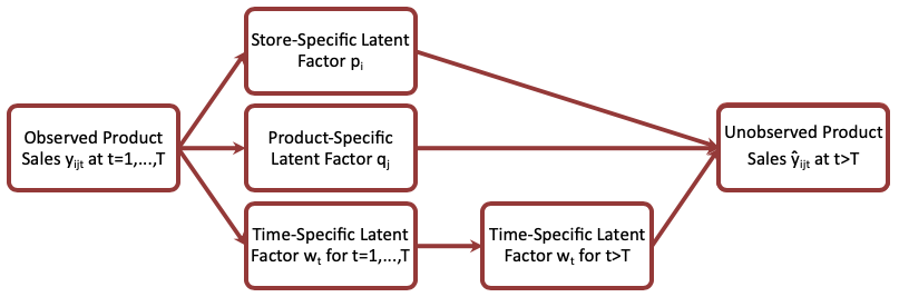
Figure 1: High-level process of the proposed method (ATLAS). Store-, product-, and time-specific latent factors are obtained from the tensor decomposition. A time-series model is applied to extrapolate time-specific factors to future time points ($t>T$). The new time-specific latent factors, together with the original store- and product-specific latent factors, are utilized to predict future sales.

One major advantage of tensor decomposition is that we convert a problem of analyzing millions of time series (e.g., combinations of thousands of stores and thousands of products) to a problem of analyzing a $k$-dimensional time series ${\bf w}_{t}$, where usually $k\leq 100$. Some existing approaches can be applied to extrapolate ${\bf w}_{t}$ from $t\leq T$ to $t>T$, for example, the kernel methods (Koren, 2010a, ), Holt-Winters method (Dunlavy et al.,, 2011), vector autoregression (Wang et al., 2016b, ), or context assertion (Hasan et al.,, 2017). Second, sales data contain a large percentage of “missing values” where stores may have little or no records of selling certain products. Using time-specific latent factors can borrow data information from similar stores or products, and hence reduce the impact of missing data. Both of these advantages are also noted in Yu et al., (2016).

To demonstrate this point, we aggregated store- and product-level IRI data into region- and category-level, respectively, such that sales competition across regions or categories is light and that sales for all region-category-week combinations are observed. Then we find that applying tensor decomposition prior to a time series model is 3% more accurate and 49% faster than applying time series models to each combination individually.

In this article, we consider two canonical and comprehensive time series models for forecasting. One is the SARIMA model (e.g.; Wei,, 1994). The other is the LSTM neural network (Hochreiter and Schmidhuber,, 1997; Gers et al.,, 1999). Technical details on how SARIMA and LSTM work are provided in Appendices 3 and 4 of the supplementary materials, respectively.

For an arbitrary time series $\{x_{t}\}_{t=1}^{T}$, both SARIMA and LSTM take $x_{1},\ldots,x_{T}$ as the input, and output $x_{T+1},\ldots,x_{T+\Delta}$ for a small number $\Delta>0$. For the proposed tensor decomposition method, we apply SARIMA or LSTM to each time series $\{w_{tl}\}$, $l=1,\ldots,k$, and acquire its forecasting value at $t>T$. Then the sales at $t=T+1,\ldots,T+\Delta$ can be predicted as

$$\hat{y}_{ijt}=\sum_{l=1}^{k}\hat{p}_{il}\hat{q}_{jl}\hat{w}_{tl}.$$ (14)

In summary, ATLAS is achieved through two steps. The first step utilizes tensor decomposition to provide store-, product-, and time-specific latent factors. In the second step, while maintaining the store- and product-specific latent factors unchanged, we extrapolate time-specific latent factors to future time points. Then we forecast future sales through using all latent factors via (14). Algorithm 1 summarizes the entire ATLAS method. For the $u$-th iteration, the improvement of the criterion function $J$ is defined as $J=1-L({\bf P}^{(u)},{\bf Q}^{(u)},{\bf W}^{(u)})/L({\bf P}^{(u-1)},{\bf Q}^{(u-1)},{\bf W}^{(u-1)})$, where $L({\bf P},{\bf Q},{\bf W})$ is defined in (8).

Data: $\lambda_{1}$, $\lambda_{1}^{*}$, $\lambda_{2}$, $k$, $\Delta$, and initial values of $J$, $\hat{p}_{i}$, $\hat{q}_{j}$, and $\hat{w}_{t}$, $t=1,\ldots,T$

Result: $\hat{y}_{ijt}$ for $i=1,\ldots,n$, $j=1,\ldots,m$ and $t=T+1,\ldots,T+\Delta$

while $J>1\times 10^{-3}$ do

       1: Estimate $\hat{{\bf P}}_{g}$ for each store group $g$ through (10),

      2: Estimate $\hat{{\bf Q}}_{d}$ for each product group $d$ through (12),

      3: Estimate $\hat{{\bf w}}_{t}$, $t=1,\ldots,T$, through (9),

end while

4: Apply SARIMA or LSTM to each time series $\{\hat{w}_{tl}\}_{t=1}^{T}$, $l=1,\ldots,k$

5. Predict $\hat{{\bf w}}_{t}$ at $t=T+1,\ldots,T+\Delta$

6: Calculate each $\hat{y}_{ijt}$ through (14)

Algorithm 1 ATLAS with Forecasting

3.4 Model Extensions

3.4.1 End-to-End Learning

One important extension of the proposed method is its ability to be formulated as an end-to-end predictive modeling technique (e.g., Wang et al.,, 2015; Wang et al., 2016a, ). As illustrated in Algorithm 1, the current version of ATLAS achieves tensor decomposition and time series analysis in two steps. An end-to-end version of ATLAS allows simultaneous achievement of these two steps. This makes the implementation of ATLAS more efficient, and, practically, may impose fewer technicalities for business analysts.

Specifically, instead of minimizing a criterion function $L({\bf P},{\bf Q},{\bf W})$ as in (8), we are now minimizing a new criterion function $L({\bf P},{\bf Q},{\bf W},\mbox{\boldmath$\theta$})$ described as follows

$$\begin{aligned} L({\bf P},{\bf Q},{\bf W},\mbox{\boldmath$\theta$})=&\sum_{(i,j,t)\in\Omega}(y_{ijt}-\sum_{l=1}^{k}p_{il}q_{jl}w_{tl})^{2}\\ &+\lambda_{1}\sum_{g=1}^{G}f_{g}+\lambda_{1}^{*}\sum_{d=1}^{D}h_{d}+\lambda_{2}(\sum_{i=1}^{n}\|{\bf p}_{i}\|^{2}+\sum_{j=1}^{m}\|{\bf q}_{j}\|^{2}+\sum_{t=1}^{T}\|{\bf w}_{t}\|^{2})\\ &+\lambda_{3}\sum_{t=\Delta_{0}+1}^{T}\|{\bf w}_{t}-\xi({\bf w}_{t-1},\ldots,{\bf w}_{t-\Delta_{0}}|\mbox{\boldmath$\theta$})\|^{2},\end{aligned}$$

where $\xi(\cdot|\mbox{\boldmath$\theta$})$ is the forecasting model approximated by either SARIMA or LSTM, $\theta$ is a vector of all parameters introduced during the training of $\xi(\cdot|\mbox{\boldmath$\theta$})$ (e.g., auto-regressive and moving-average coefficients in SARIMA, or weight matrices and bias vectors in LSTM), $\Delta_{0}>0$ is the prespecified time lag, and $\lambda_{3}>0$ is a new tuning parameter.

We still consider the blockwise coordinate descent algorithm when optimizing the criterion function above. In other words, parameters $({\bf P},{\bf Q},{\bf W},\mbox{\boldmath$\theta$})$ are estimated cyclically, where the estimation of ${\bf P},{\bf Q},{\bf W}$ follows (10), (12), and (9), respectively, and the estimation of $\theta$ is provided by either SARIMA or LSTM. Numerical results of this end-to-end version of ATLAS are provided in Appendix 5 of the supplementary materials. Importantly, the original and end-to-end versions of ATLAS provide highly similar forecasting performance.

3.4.2 Incorporating Contextual Information

Another important extension is to incorporate contextual information that could have a direct impact on sales; our proposed approach is able to incorporate this aspect naturally, as part of the pre-model-building preparation. In particular, suppose we observe a vector of independent variables ${\bf x}_{ijt}$. For example, elements of ${\bf x}_{ijt}$ may represent the price, and promotion, managerial, and operational strategies of product $j$ in store $i$ at time $t$. Then we can fit a linear regression to control the effects of variables in ${\bf x}$ before applying ATLAS. In other words, we define $e_{ijt}=y_{ijt}-{\bf x}_{ijt}\hat{\mbox{\boldmath$\beta$}},$ where $\hat{\mbox{\boldmath$\beta$}}$ is the estimated regression coefficient of $y_{ijt}$’s fitted against ${\bf x}_{ijt}$’s. Next, we replace each $y_{ijt}$ by $e_{ijt}$, and conduct Algorithm 1 to forecast $\hat{e}_{ijt}$’s for $t=T+1,\ldots,T+\Delta$. Then the final context-aware forecast can be obtained as

$$\hat{y}_{ijt}={\bf x}_{ijt}\hat{\mbox{\boldmath$\beta$}}+\hat{e}_{ijt},\mbox{ for }t=T+1,\ldots,T+\Delta.$$

Incorporating contextual information brings two advantages. First, from a managerial perspective, through fitting a regression model, managers could know which factors are significant contributors to sales, as well as how these factors are influencing the sales amount. This allows managers to design more informed pricing and promotion strategies. Second, from a technical perspective, incorporating contextual information may improve forecasting accuracy. Along this direction, we could also consider deep learning techniques such as feedforward neural networks or embedding approaches to further enhance the forecasting results. Numerical experiments on IRI data incorporating price and promotion information are conducted and provided in Appendix 6 of the supplementary materials.

4 A Real-World Application: IRI Marketing Data

4.1 Data Description

In our study, we use the IRI marketing data as an example to demonstrate the effectiveness of the proposed method. The data we acquired are from 2008 to 2011 at a weekly level of granularity (i.e., 208 weeks in total). Specifically, the dataset contains weekly transactions of 2,447 grocery stores from over 47 U.S. markets. A detailed description of an early version (2001-2005) of the data, as well as the data’s availability, can be obtained from Bronnenberg et al., (2008). Figure 2 illustrates a snapshot of the original data. Here the first column is the de-identified store ID. Notice that, although the data are collected at the store level, all stores in the datasets are chain (rather than independent) stores. Bronnenberg et al., (2008) provide the rationale that independent stores “are less important for competition in most markets.” This also aligns with our research goal where important competitors are included in the forecasting. Zipcode of each store is also provided in a separate spreadsheet. The second column represents the week ID, where 1479 corresponds to the first week of 2008 (i.e., December 31, 2007 to January 6, 2008) and 1686 corresponds to the second-to-last week of 2011 (i.e., December 19, 2011 to December 25, 2011, the last week that our data are collected). Columns 3-6 (i.e., system code, product generation, vendor ID, item ID) together make up a twelve-digit Universal Product Code (UPC) which is unique for each product and thus is used as the product ID in our analysis. In the last two columns, the volume and dollar amount of sales of each product are recorded. For example, in the first row in Figure 2, store #234212 has sold 1 unit of product #0-1-41778-08268 in week #1479 for 9.99 dollars.

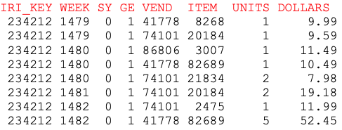
Figure 2: A snapshot of the IRI data.

Due to the fact that many products come in different sizes but may share the same unit (for example, beverages may come in one single bottle or a six-pack, selling either one of which would be counted as a 1-unit sale, but essentially they are very different), we therefore choose dollar amount as the response variable for analysis and forecasting. Nevertheless, we are aware of the importance of sales units in the sales forecasting area. The proposed method, as well as all the competing methods, can be applied to the sales unit forecasting if they are tuned accordingly.

Data from eight categories of products are analyzed, including razor blades, coffee, deodorant, diapers, frozen pizza, milk, photography related products, and toothpaste. That is, a spreadsheet similar to Figure 2 is collected for each product category. The proposed method, as well as its competing methods, are applied to each product category individually and compared. In other words, the eight categories are treated as eight independent datasets for the forecasting purposes.

In Table 1, we list the number of grocery stores, number of products, and sample size (number of rows as in Figure 2) within each category. For every category, we select stores or products only if they have more than 1,000 or 200 transactions, respectively. That is, on an average week, a selected store sells at least 5 products, and a selected product is sold in at least one store across the entire nation. We also demonstrate in Appendix 7 of the supplementary materials that the performance of ATLAS does not change substantially if all stores and products are included.

The number of stores is similar across all datasets except for the photography category. In terms of the number of products, nearly 5,000 coffee products and 4,000 milk products nationwide pass the aforementioned screening. The sample size of each category ranges from 0.2 million to nearly 39 million. However, although the sample size for most datasets is large, there are still a huge number of store-product-week combinations that do not have any sales. For example, there are 1,528 stores that sell milk, 3,739 types of milk, and a total of 208 weeks. The total number of store-product-week combinations could go up to $1528\times 3739\times 208\approx 1.2\mbox{ billion}$. In contrast, the sample size of 26.4 million observed milk-related combinations, although large, is still highly sparse in the store-product-week tensor, as it only consists of roughly $2.2\%$ of the total elements.

Table 1: The number of grocery stores, number of products, and the sample size (number of rows as in Figure 2) are provided for each dataset we analyze.

	Num. of Stores	Num. of Products	Sample Size
Blades	1,417	686	9,001,597
Coffee	1,535	4,844	38,971,593
Deodorant	1,502	1,445	25,869,335
Diapers	1,477	1,653	13,622,073
Frozen Pizza	1,528	2,057	28,574,874
Milk	1,528	3,739	26,439,459
Photography	176	131	241,851
Tooth Paste	1,511	1,005	22,173,211

In Appendix 8 of the supplementary materials, we provide the summary statistics regarding the average sales amount of each single product (per store per week) for each dataset, as well as the weekly sales trends of the eight categories of products.

Since all the participating stores are grocery stores, we expect that local consumer demand dynamics exists among stores in close proximity. Therefore, we consider a store group as a geographical region defined by the 3-digit zip code prefix. As an illustration, in each panel of Figure 3, we have identified a region in the Northeastern U.S. where only two chain stores were selling milk. In the left panel, store #906 and #1255 were the only two chain stores in the region. Store #906 closed (or stopped selling milk) near the end of year 2010, and since then store #1255 saw an increase in milk sales. In the right panel, store #695 was once the only chain store in that region which sold milk. A new store, #1264, opened (or started to sell milk) since spring 2011 whose sales amount started to increase by the end of summer 2011. Then we saw a slightly decrease in the milk sales in the existing store #695. However, product specific attributes (such as subcategory or volume) are not available in our datasets. Therefore, product demand dynamics is not considered in our numerical studies. In the Discussion section, we discuss this direction as an important future research area.

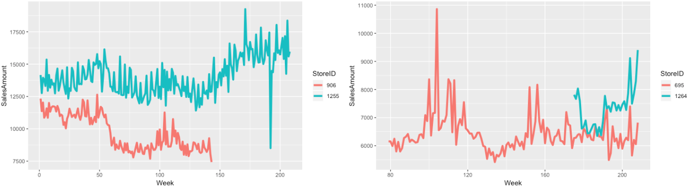
Figure 3: Sales amounts of milk changed after the opening or closing of the sole competitor in the same region.

4.2 Model Description

The proposed method is compared to seven methods from prior literature. One is the classical and widely-adopted time-series benchmark: the SARIMA model. We apply it to every store-product pair individually. In other words, a 208-week time series of sales amounts is analyzed for every single product in every single store without requiring data of other stores (or products). Another two methods are LSTM and vector autoregression (VAR; e.g., Holtz-Eakin et al.,, 1988) which can formulate multivariate time series.

The other three methods are more recent and competitive latent factor models which have frameworks similar to the one of ATLAS and have demonstrated or claimed their capability of sales forecasting under the same or similar scenarios, i.e., where sales across multiple stores and products are available. Specifically, they are Bayesian probabilistic tensor factorization (BPTF; Xiong et al.,, 2010), factorization machine (libFM; Rendle,, 2012), and temporal regularized matrix factorization (TRMF; Yu et al.,, 2016). However, none of them consider local demand information in the latent factor estimation step. And while some of them consider extrapolation, none of them incorporate full SARIMA, or LSTM as canonical tools for forecasting. For VAR, LSTM, and TRMF, we apply them to each store individually, while for the rest of the latent factor models, we formulate all stores and products simultaneously.

In addition, we also report the results of ATLAS without incorporating local demand dynamics, namely, CP decomposition (CPD) with SARIMA or LSTM, through which we demonstrate that incorporating local demand dynamics indeed improves the forecasting accuracy. For the proposed method as well as most of the latent factor benchmarks, we expect sufficient observations from stores, products, or weeks (ideally close to or greater than the number of latent factors $k$ for each of them), such that the estimation procedures can be robust. This has been met in the IRI datasets.

4.3 Model Training and Validation

Recall that data from a total of 208 weeks are collected, and our ultimate goal is to forecast the future sales amounts based on historical sales data. Therefore, we split the training, validation, and testing set based on the chronological order, rather than a random split, to mimic the real-world forecasting scenario. Unlike in many applications where a series of rolling one-point-ahead forecasting is adopted (e.g.; Osadchiy et al.,, 2013), retail sales usually expect a longer-term forecasting for the sake of optimizing their operational decisions (Cui et al.,, 2018). Therefore, we use data from the first 192 weeks as the training set, weeks 193-200 as the validation set, and the latest 8 weeks as the testing set (see Figure 4 for an illustration). Summary of the training, validation, and test data, as well as detailed information about parameter tuning, its managerial interpretation, and model software availability, are provided in Appendices 9 and 10 of the supplementary materials. Here the 8-week-ahead forecasting window was determined after some discussions with a few local experts, who are in retail business, subscribe to the IRI marketing data, and conduct sales forecasting on a regular basis. The length of forecasting horizon, however, can be adjusted based on different contexts or needs. To evaluate the performance of ATLAS on different forecasting horizons, we allow a varying test data size (ranging from 4 to 20 weeks) in Appendix 12 of the supplementary materials, where ATLAS is compared with competing methods and demonstrates advantageous performance. We further conduct an additional experiment for robustness check in Appendix 13, where we evaluate ATLAS under different training data size (ranging from 8 to 192 weeks) to demonstrate its stability when the time range of training data collection is short.

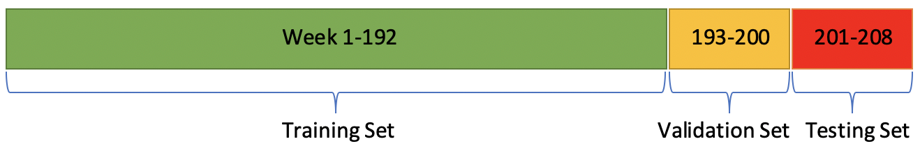
Figure 4: Each dataset is split into a training set (week 1-192), a validation set (week 193-200) and a testing set (week 201-208), based on the chronological order.

5 Main Results: Product Sales Forecasting

In this section, we apply ATLAS and competing methods to the eight IRI marketing datasets described in Section 4.1.

5.1 Performance Evaluation

For model performance evaluation, we utilize the popular and widely used numeric prediction accuracy metric – root mean square error (RMSE), which assigns disproportionately larger penalties for bigger prediction errors. Suppose $y_{ijt}$ is the sales amount of product $j$ in store $i$ at week $t$, and $\hat{y}_{ijt}$ is the predicted value of $y_{ijt}$. Then the RMSE on a given test set $\Omega$ is defined as $\mbox{RMSE}(\Omega)=\left\{\frac{1}{|\Omega|}\sum_{(i,j,t)\in\Omega}(y_{ijt}-\hat{y}_{ijt})^{2}\right\}^{1/2},$ where $\Omega=\{(i,j,t):y_{ijt}\mbox{ is observed and }t>200\}$ in the IRI data context, and $|\Omega|$ is the size of $\Omega$.

In Table 2, we list the RMSE values exhibited by ATLAS and the competing methods. Smaller RMSE indicates a smaller average distance between the predicted and the actual sales amounts. The differences in the results of CPD with SARIMA or LSTM are less than $10^{-4}$, and hence are reported as one column.

In general, ATLAS (either with SARIMA or LSTM) demonstrates the best performance across all product categories: ATLAS with SARIMA forecasting has the best performance in seven out of eight datasets, and ATLAS with LSTM forecasting has the best performance in the deodorant dataset. It is possible that given a longer time series, LSTM would be able to achieve better performance. And in many categories, both ATLAS with SARIMA and ATLAS with LSTM perform better than the competing methods (or at least in the top 3). It is important to note that, for VAR, the number of parameters is huge, which results in overfitting and sometimes unreasonably large predicted values for stores with few transaction records. To alleviate this issue and significantly improve the VAR predictive performance, we truncate the most extreme 10% of VAR results, that is, replacing the largest (and smallest) 5% predicted values by the 95th (and 5th) quantile. In particular, by comparing the results of CPD and ATLAS, we can see that incorporating local consumer demand dynamics indeed improves prediction accuracy. In Appendix 11 of the supplementary materials, we also consider performance evaluation under the mean absolute error metric, where ATLAS also demonstrates superior performance for the vast majority of datasets.

To further evaluate the performance of ATLAS across product categories, we combine “coffee” and “milk”, as they both belong to beverages. We also combine “blades” and “toothpaste”, as they both represent personal hygiene products. Furthermore, we combine “coffee”, “milk”, and “frozen pizza” as “edibles”, and “blades”, “deodorant”, “diapers”, “photography”, and “tooth paste” as “inedibles”. We demonstrate in Appendix 14 of the supplementary materials that, for products in categories which are more likely to be co-purchased, such as “coffee” and “milk”, ATLAS is able to take advantage of the additional across-category information and further enhance its forecasting accuracy. In Appendix 15, we further compare ATLAS with competing methods after aggregating the original product-level data into completely category-level data (i.e., no more product-specific transactions), which significantly reduces data sparsity (i.e., much less data are “missing” at the store-category level). Advantageous performance of ATLAS is still observed, indicating its flexibility on datasets with varying degrees of density.

Table 2: RMSE results from the proposed method with SARIMA forecasting (ALTLAS(S)) and with LSTM forecasting (ATLAS(L)) are compared with baseline techniques, where VAR and LSTM are new benchmarks; the lowest RMSE for each category is highlighted in bold.

	SARIMA	VAR	LSTM	BPTF	libFM	TRMF	CPD	ATLAS(S)	ATLAS(L)
Blades	17.09	25.91	18.53	16.75	21.03	17.65	17.17	14.26	14.32
Coffee	60.47	69.14	56.08	72.06	54.83	61.97	59.03	52.32	57.19
Deodorant	8.12	7.96	6.94	9.48	5.92	7.23	5.57	5.72	5.54
Diapers	30.01	27.53	26.10	25.38	16.34	25.48	17.31	15.67	16.20
Frozen Pizza	41.46	47.37	35.77	42.51	105.75	43.00	39.33	33.92	34.41
Milk	103.19	336.44	119.09	204.31	349.70	108.85	226.69	78.91	85.20
Photography	11.77	12.85	12.55	12.61	12.27	11.94	12.04	10.66	11.20
Tooth Paste	35.62	21.00	18.96	48.25	28.38	22.98	18.18	17.17	18.60

5.2 Efficiency

In terms of computational efficiency, all the latent factor models are significantly faster than the individual SARIMA, since the sales across multiple stores and products are modeled simultaneously. Theoretically, BPTF, libFM, CPD, and ATLAS have the same computational complexity in terms of the number of stores, products, and weeks, as all of them estimate the three modes of a tensor iteratively and their loss functions have similar forms with explicit solutions. TRMF, VAR, and LSTM are applied to each store individually, and are hence slower than the tensor based methods. In general, the computational complexity of each method is provided in Table 3. When the number of stores and products are large, BPTF, libFM, CPD, and ATLAS are expected to have high computational efficiency.

Table 3: Computational complexity of the tensor decomposition of ALTAS is compared with baseline techniques. Here $n_{s}$, $n_{p}$ and $n_{w}$ represent the number of stores, products, and weeks, respectively.

ARIMA	TRMF, VAR and LSTM	ATLAS and others
$O(n_{s}n_{p}n_{w})$	$O(n_{s}(n_{p}+n_{w}))$	$O(n_{s}+n_{p}+n_{w})$

In practice, however, the computational runtime (model building and deployment) may differ, as the best-performing model parameters, convergence criterion, and number of iterations might be pre-specified differently. For example, for the frozen pizza dataset, the computational runtimes for individual SARIMA, VAR, LSTM, BPTF, libFM, TRMF, CPD, and ATLAS were 28.07, 9.13, 1.62, 0.80, 0.93, 5.91, 0.42, and 1.83 hours, respectively. And for the toothpaste dataset, the computational runtimes for individual SARIMA, VAR, LSTM, BPTF, libFM, TRMF, CPD, and ATLAS were 18.49, 10.90, 8.55, 0.42, 0.79, 4.51, 0.23, and 0.81 hours, respectively. It can be seen that the computational runtimes for each method roughly follow the theoretical complexity as provided in Table 3, where SARIMA is the longest, followed by VAR, LSTM, and TRMF, while BPTF, libFM, CPD, and ATLAS are at comparable levels.

6 Summary and Conclusions

Following the design science paradigm, we propose, develop, and evaluate a new latent-factor-based approach, namely the Advanced Temporal Latent-factor Approach to Sales forecasting (ATLAS). Specifically, ATLAS is designed for the complex settings where sales data from multiple stores across multiple products are collected, and sales forecasting for many store-product combinations is of interest. The key feature of our work is that ATLAS is able to incorporate elements of local consumer demand information in a large-scale, multiple-store, multiple-product setting. It leads to significant accuracy improvements, especially compared with existing latent factor models which use a similar framework. Such accuracy improvement on sales forecasting provides important managerial implications for companies’ decision making for budgeting, production, supply chain management, and inventory control.

This work opens up several interesting opportunities for future studies. Although the proposed model improves upon existing methods through incorporation of local demand dynamics as part of its regularization procedure, it does not attempt to model the consumer demand directly, e.g., based on sophisticated economic theory. While the current approach does provide substantial forecasting accuracy improvements, we believe that incorporating economic theory considerations into machine learning models can provide significant additional advantages, and, thus, constitutes a promising direction for future work. For instance, from a microeconomic perspective, the consumer demand might be formulated by the consumer choice models as in demand theory (Böhm and Haller,, 2008). Collecting data at the customer level and incorporating consumer choice models into the tensor framework might lead to further improvements in forecasting accuracy.

Second, refining the definition of the demand dynamics may further improve flexibility and forecasting accuracy of the proposed model. For example, there could be asymmetric competition among stores or products, which may not be formulated as correlation matrices. Therefore, new regularization methods to accommodate asymmetric matrices are needed. Furthermore, a time-dependent demand formulation may be considered. This requires the estimation of time-varying parameters as well as imposes additional assumptions regarding how the covariance matrix would change in the near future. To address this issue, one possible solution is to allow the demand dynamics to change less rapidly, for example, on a seasonal or yearly basis, based on domain knowledge, such that fewer new parameters are needed while the demand pattern is no longer static. Meanwhile, we are also aware that there may be other store competitors, both online and offline, which can be considered if their data become available.

Finally, there can be additional socioeconomic, marketing, managerial, operational, and product-related attributes which contribute to the forecasting results. For example, the IRI dataset provides demographic information of the population within 2-mile radius of each store location, which includes, for example, number of households, average age, percentage of males/females, and average household income. Incorporating this information may further explain demand dynamics and enhance sales forecasting. Furthermore, it would be interesting to explore which specific products (or what specific characteristics of products) favor ATLAS. Collecting product-related information may help address this issue and provide deeper managerial implications regarding where and how the proposed method may be most advantageous. Meanwhile, if other variables, such as managerial and operational strategies are available, one may consider generalizing the proposed approach even further to utilize this information.

References

- Adomavicius et al., (2013) Adomavicius, G., Bockstedt, J., Curley, S. P., and Zhang, J. (2013). Do recommender systems manipulate consumer preferences? A study of anchoring effects. Information Systems Research, 24(4):956–975.
- Adomavicius et al., (2018) Adomavicius, G., Bockstedt, J. C., Curley, S. P., and Zhang, J. (2018). Effects of online recommendations on consumers’ willingness to pay. Information Systems Research, 29(1):84–102.
- Adomavicius and Kwon, (2014) Adomavicius, G. and Kwon, Y. (2014). Optimization-based approaches for maximizing aggregate recommendation diversity. INFORMS Journal on Computing, 26(2):351–369.
- Adomavicius and Tuzhilin, (2005) Adomavicius, G. and Tuzhilin, A. (2005). Toward the next generation of recommender systems: A survey of the state-of-the-art and possible extensions. IEEE Transactions on Knowledge and Data Engineering, 17(6):734–749.
- Adomavicius and Tuzhilin, (2015) Adomavicius, G. and Tuzhilin, A. (2015). Context-aware recommender systems. In Recommender Systems Handbook, 191–226. Springer.
- Aggarwal, (2016) Aggarwal, C. C. (2016). Recommender Systems. Springer.
- Bell and Koren, (2007) Bell, R. M. and Koren, Y. (2007). Scalable collaborative filtering with jointly derived neighborhood interpolation weights. In Proceedings of the 2007 7th IEEE International Conference on Data Mining, 43–52. IEEE.
- Bi et al., (2018) Bi, X., Qu, A., and Shen, X. (2018). Multilayer tensor factorization with applications to recommender systems. The Annals of Statistics, 46(6B):3308–3333.
- Bi et al., (2017) Bi, X., Qu, A., Wang, J., and Shen, X. (2017). A group specific recommender system. Journal of the American Statistical Association, 112(519):1344–1353.
- (10) Bi, X., Tang, X., Yuan, Y., Zhang, Y., and Qu, A. (2020a). Tensors in statistics. Annual Review of Statistics and Its Application, 8.
- (11) Bi, X., Yang, M., and Adomavicius, G. (2020b). Consumer acquisition for recommender systems: A theoretical framework and empirical evaluations. Available at SSRN.
- Böhm and Haller, (2008) Böhm, V. and Haller, H. (2008). Demand theory. The New Palgrave Dictionary of Economics, 2:1311–1320.
- Box et al., (2015) Box, G. E., Jenkins, G. M., Reinsel, G. C., and Ljung, G. M. (2015). Time Series Analysis: Forecasting and Control. John Wiley & Sons, 5th edition.
- Breese et al., (1998) Breese, J. S., Heckerman, D., and Kadie, C. (1998). Empirical analysis of predictive algorithms for collaborative filtering. In Proceedings of the Fourteenth Conference on Uncertainty in Artificial Intelligence, 43–52. Morgan Kaufmann Publishers Inc.
- Bronnenberg et al., (2008) Bronnenberg, B. J., Kruger, M. W., and Mela, C. F. (2008). Database paper-The IRI marketing data set. Marketing Science, 27(4):745–748.
- Brynjolfsson et al., (2011) Brynjolfsson, E., Hu, Y., and Simester, D. (2011). Goodbye pareto principle, hello long tail: The effect of search costs on the concentration of product sales. Management Science, 57(8):1373–1386.
- Brynjolfsson et al., (2010) Brynjolfsson, E., Hu, Y., and Smith, M. D. (2010). Research commentary—long tails vs. superstars: The effect of information technology on product variety and sales concentration patterns. Information Systems Research, 21(4):736–747.
- Campos et al., (2014) Campos, P. G., Díez, F., and Cantador, I. (2014). Time-aware recommender systems: a comprehensive survey and analysis of existing evaluation protocols. User Modeling and User-Adapted Interaction, 24(1-2):67–119.
- Carroll and Chang, (1970) Carroll, J. D. and Chang, J.-J. (1970). Analysis of individual differences in multidimensional scaling via an N-way generalization of “Eckart-Young” decomposition. Psychometrika, 35(3):283–319.
- Chen and Xie, (2005) Chen, Y. and Xie, J. (2005). Third-party product review and firm marketing strategy. Marketing Science, 24(2):218–240.
- Choi et al., (2018) Choi, T.-M., Wallace, S. W., and Wang, Y. (2018). Big data analytics in operations management. Production and Operations Management, 27(10):1868–1883.
- Chong et al., (2017) Chong, A. Y. L., Ch’ng, E., Liu, M. J., and Li, B. (2017). Predicting consumer product demands via big data: the roles of online promotional marketing and online reviews. International Journal of Production Research, 55(17):5142–5156.
- Chu and Cao, (2011) Chu, B.-S. and Cao, D.-B. (2011). Dynamic cubic neural network with demand momentum for new product sales forecasting. Information-An International Interdisciplinary Journal, 14(4):1171–1182.
- Clark and Provost, (2016) Clark, J. and Provost, F. (2016). Matrix-factorization-based dimensionality reduction in the predictive modeling process: A design science perspective. NYU Working Paper No.; CBA-16-01.
- Cui et al., (2018) Cui, R., Gallino, S., Moreno, A., and Zhang, D. J. (2018). The operational value of social media information. Production and Operations Management, 27(10):1749–1769.
- Curtis et al., (2014) Curtis, A., Lundholm, R. J., and McVay, S. E. (2014). Forecasting sales: A model and some evidence from the retail industry. Contemporary Accounting Research, 31(2):581–608.
- Dunlavy et al., (2011) Dunlavy, D. M., Kolda, T. G., and Acar, E. (2011). Temporal link prediction using matrix and tensor factorizations. ACM Transactions on Knowledge Discovery from Data (TKDD), 5(2):10.
- Ferreira et al., (2015) Ferreira, K. J., Lee, B. H. A., and Simchi-Levi, D. (2015). Analytics for an online retailer: Demand forecasting and price optimization. Manufacturing & Service Operations Management, 18(1):69–88.
- Feuerverger et al., (2012) Feuerverger, A., He, Y., and Khatri, S. (2012). Statistical significance of the Netflix challenge. Statistical Science, 27(2):202–231.
- Fisher et al., (2018) Fisher, M., Gallino, S., and Li, J. (2018). Competition-based dynamic pricing in online retailing: A methodology validated with field experiments. Management Science, 64(6):2496–2514.
- Fleder and Hosanagar, (2009) Fleder, D. and Hosanagar, K. (2009). Blockbuster culture’s next rise or fall: The impact of recommender systems on sales diversity. Management Science, 55(5):697–712.
- Friedman et al., (2007) Friedman, J., Hastie, T., Höfling, H., and Tibshirani, R. (2007). Pathwise coordinate optimization. The Annals of Applied Statistics, 1(2):302–332.
- Funk, (2006) Funk, S. (2006). Netflix update: Try this at home. URL http://sifter.org/~simon/journal/20061211.html.
- Gaur et al., (2007) Gaur, V., Kesavan, S., Raman, A., and Fisher, M. L. (2007). Estimating demand uncertainty using judgmental forecasts. Manufacturing & Service Operations Management, 9(4):480–491.
- Gers et al., (1999) Gers, F. A., Schmidhuber, J., and Cummins, F. (1999). Learning to forget: Continual prediction with LSTM. Proceedings of ICANN’99 International Conference on Artificial Neural Networks, 2:850–855.
- Giering, (2008) Giering, M. (2008). Retail sales prediction and item recommendations using customer demographics at store level. ACM SIGKDD Explorations Newsletter, 10(2):84–89.
- Graves et al., (2008) Graves, A., Liwicki, M., Fernández, S., Bertolami, R., Bunke, H., and Schmidhuber, J. (2008). A novel connectionist system for unconstrained handwriting recognition. IEEE Transactions on Pattern Analysis and Machine Intelligence, 31(5):855–868.
- Harshman, (1970) Harshman, R. A. (1970). Foundations of the PARAFAC procedure: Models and conditions for an "explanatory" multi-modal factor analysis. UCLA Working Papers in Phonetics, 16:1–84.
- Hasan et al., (2017) Hasan, T., Arshad, N., Dahquist, E., and McCrickard, S. (2017). Collaborative filtering for household load prediction given contextual information. SDM ’17 Workshop on Machine Learning for Recommender Systems.
- Hevner et al., (2004) Hevner, A. R., March, S. T., Park, J., and Ram, S. (2004). Design science in information systems research. MIS Quarterly, 28(1):75–105.
- Hidasi and Tikk, (2012) Hidasi, B. and Tikk, D. (2012). Fast als-based tensor factorization for context-aware recommendation from implicit feedback. In Joint European Conference on Machine Learning and Knowledge Discovery in Databases, 67–82. Springer.
- Hochreiter and Schmidhuber, (1997) Hochreiter, S. and Schmidhuber, J. (1997). Long short-term memory. Neural computation, 9(8):1735–1780.
- Holtz-Eakin et al., (1988) Holtz-Eakin, D., Newey, W., and Rosen, H. S. (1988). Estimating vector autoregressions with panel data. Econometrica, 1371–1395.
- Horrigan, (2016) Horrigan, J. B. (2016). Information overload. Pew Research Center.
- Hosanagar et al., (2014) Hosanagar, K., Fleder, D., Lee, D., and Buja, A. (2014). Will the global village fracture into tribes? Recommender systems and their effects on consumer fragmentation. Management Science, 60(4):805–823.
- Jacoby, (1984) Jacoby, J. (1984). Perspectives on information overload. Journal of consumer research, 10(4):432–435.
- Jahrer et al., (2010) Jahrer, M., Töscher, A., and Legenstein, R. (2010). Combining predictions for accurate recommender systems. In Proceedings of the 16th ACM SIGKDD international conference on Knowledge discovery and data mining, 693–702. ACM.
- Kaneko and Yada, (2016) Kaneko, Y. and Yada, K. (2016). A deep learning approach for the prediction of retail store sales. In 2016 IEEE 16th International Conference on Data Mining Workshops (ICDMW), 531–537. IEEE.
- Karatzoglou et al., (2010) Karatzoglou, A., Amatriain, X., Baltrunas, L., and Oliver, N. (2010). Multiverse recommendation: n-dimensional tensor factorization for context-aware collaborative filtering. In Proceedings of the Fourth ACM Conference on Recommender Systems, 79–86. ACM.
- Kesavan et al., (2010) Kesavan, S., Gaur, V., and Raman, A. (2010). Do inventory and gross margin data improve sales forecasts for U.S. public retailers? Management Science, 56(9):1519–1533.
- Kiros et al., (2014) Kiros, R., Salakhutdinov, R., and Zemel, R. S. (2014). Unifying visual-semantic embeddings with multimodal neural language models. arXiv:1411.2539.
- Koenigstein et al., (2011) Koenigstein, N., Dror, G., and Koren, Y. (2011). Yahoo! music recommendations: modeling music ratings with temporal dynamics and item taxonomy. In Proceedings of the fifth ACM conference on Recommender systems, 165–172. ACM.
- (53) Koren, Y. (2010a). Collaborative filtering with temporal dynamics. Communications of the ACM, 53(4):89–97.
- (54) Koren, Y. (2010b). Factor in the neighbors: Scalable and accurate collaborative filtering. ACM Transactions on Knowledge Discovery from Data (TKDD), 4(1):1.
- Koren and Bell, (2015) Koren, Y. and Bell, R. (2015). Advances in collaborative filtering. In Recommender Systems Handbook, 77–118. Springer.
- Koren et al., (2009) Koren, Y., Bell, R., and Volinsky, C. (2009). Matrix factorization techniques for recommender systems. Computer, 42(8):30–37.
- Kremer et al., (2011) Kremer, M., Moritz, B., and Siemsen, E. (2011). Demand forecasting behavior: System neglect and change detection. Management Science, 57(10):1827–1843.
- Lau et al., (2018) Lau, R. Y. K., Zhang, W., and Xu, W. (2018). Parallel aspect-oriented sentiment analysis for sales forecasting with big data. Production and Operations Management, 27(10):1775–1794.
- Lee and Hosanagar, (2019) Lee, D. and Hosanagar, K. (2019). How do recommender systems affect sales diversity? A cross-category investigation via randomized field experiment. Information Systems Research, to appear.
- Li and Wu, (2015) Li, X. and Wu, X. (2015). Constructing long short-term memory based deep recurrent neural networks for large vocabulary speech recognition. In 2015 IEEE International Conference on Acoustics, Speech and Signal Processing, 4520–4524.
- Liebman et al., (2019) Liebman, E., Saar-Tsechansky, M., and Stone, P. (2019). The right music at the right time: Adaptive personalized playlists based on sequence modeling. Management Information Systems Quarterly, to appear.
- Liu et al., (2016) Liu, X., Singh, P. V., and Srinivasan, K. (2016). A structured analysis of unstructured big data by leveraging cloud computing. Marketing Science, 35(3):363–388.
- Ma et al., (2016) Ma, S., Fildes, R., and Huang, T. (2016). Demand forecasting with high dimensional data: The case of sku retail sales forecasting with intra-and inter-category promotional information. European Journal of Operational Research, 249(1):245–257.
- Mahajan and Wind, (1988) Mahajan, V. and Wind, Y. (1988). New product forecasting models: Directions for research and implementation. International Journal of Forecasting, 4(3):341–358.
- Malhotra et al., (2015) Malhotra, P., Vig, L., Shroff, G., and Agarwal, P. (2015). Long short term memory networks for anomaly detection in time series. In Proceedings of European Symposium on Artificial Neural Networks, Computational Intelligence and Machine Learning, 89–94.
- Mas-Machuca et al., (2014) Mas-Machuca, M., Sainz, M., and Martinez-Costa, C. (2014). A review of forecasting models for new products. Intangible Capital, 10(1):1–25.
- Mentzer and Moon, (2004) Mentzer, J. T. and Moon, M. A. (2004). Sales Forecasting Management: A Demand Management Approach. Sage Publications, Inc., 2nd edition.
- Muter and Aytekin, (2017) Muter, I. and Aytekin, T. (2017). Incorporating aggregate diversity in recommender systems using scalable optimization approaches. INFORMS Journal on Computing, 29(3):405–421.
- Nichols and Tsay, (1979) Nichols, D. R. and Tsay, J. J. (1979). Security price reactions to long-range executive earnings forecasts. Journal of Accounting Research, 140–155.
- Oestreicher-Singer and Sundararajan, (2012) Oestreicher-Singer, G. and Sundararajan, A. (2012). Recommendation networks and the long tail of electronic commerce. MIS Quarterly, 36(1):65–83.
- Osadchiy et al., (2013) Osadchiy, N., Gaur, V., and Seshadri, S. (2013). Sales forecasting with financial indicators and experts’ input. Production and Operations Management, 22(5):1056–1076.
- Panniello et al., (2016) Panniello, U., Gorgoglione, M., and Tuzhilin, A. (2016). Research note—In CARSs we trust: How context-aware recommendations affect customers’ trust and other business performance measures of recommender systems. Information Systems Research, 27(1):182–196.
- Parry et al., (2011) Parry, M. E., Cao, Q., and Song, M. (2011). Forecasting new product adoption with probabilistic neural networks. Journal of Product Innovation Management, 28(s1):78–88.
- Pavlyshenko, (2019) Pavlyshenko, B. M. (2019). Machine-learning models for sales time series forecasting. Data, 4(1):15.
- Penman, (1980) Penman, S. H. (1980). An empirical investigation of the voluntary disclosure of corporate earnings forecasts. Journal of accounting research, 132–160.
- Rendle, (2012) Rendle, S. (2012). Factorization machines with libFM. ACM Transactions on Intelligent Systems and Technology, 3(3):57:1–57:22.
- Resnick et al., (1994) Resnick, P., Iacovou, N., Suchak, M., Bergstrom, P., and Riedl, J. (1994). Grouplens: An open architecture for collaborative filtering of netnews. In Proceedings of the 1994 ACM Conference on Computer Supported Cooperative Work, 175–186. ACM.
- Ricci et al., (2011) Ricci, F., Rokach, L., and Shapira, B. (2011). Introduction to recommender systems handbook. In Recommender systems handbook, 1–35. Springer.
- Rumelhart et al., (1988) Rumelhart, D. E., Hinton, G. E., Williams, R. J., et al. (1988). Learning representations by back-propagating errors. Cognitive modeling, 5(3):1.
- (80) Sahoo, N., Krishnan, R., Duncan, G., and Callan, J. (2012a). Research note—The halo effect in multicomponent ratings and its implications for recommender systems: The case of Yahoo! movies. Information Systems Research, 23(1):231–246.
- (81) Sahoo, N., Singh, P. V., and Mukhopadhyay, T. (2012b). A hidden markov model for collaborative filtering. MIS Quarterly, 36(4):1329–1356.
- Sak et al., (2014) Sak, H., Senior, A., and Beaufays, F. (2014). Long short-term memory recurrent neural network architectures for large scale acoustic modeling. In Fifteenth Annual Conference of the International Speech Communication Association.
- Salakhutdinov et al., (2007) Salakhutdinov, R., Mnih, A., and Hinton, G. (2007). Restricted Boltzmann machines for collaborative filtering. In Proceedings of the 24th International Conference on Machine Learning, 791–798. ACM.
- Sarwar et al., (2001) Sarwar, B. M., Karypis, G., Konstan, J. A., and Riedl, J. (2001). Item-based collaborative filtering recommendation algorithms. In Proceedings of the 10th International WWW Conference, volume 1, 285–295.
- Schroeder and Goldstein, (2016) Schroeder, R. G. and Goldstein, S. M. (2016). Operations Management in the Supply Chain: Decisions and Cases. McGraw-Hill Education, 7th edition.
- See-To and Ngai, (2018) See-To, E. W. and Ngai, E. W. (2018). Customer reviews for demand distribution and sales nowcasting: A big data approach. Annals of Operations Research, 270(1-2):415–431.
- Shi et al., (2015) Shi, X., Chen, Z., Wang, H., Yeung, D.-Y., Wong, W.-K., and Woo, W.-c. (2015). Convolutional LSTM network: A machine learning approach for precipitation nowcasting. In Advances in Neural Information Processing Systems, 802–810.
- Shi et al., (2017) Shi, X., Gao, Z., Lausen, L., Wang, H., Yeung, D.-Y., Wong, W.-k., and Woo, W.-c. (2017). Deep learning for precipitation nowcasting: A benchmark and a new model. In Advances in Neural Information Processing Systems, 5617–5627.
- Song et al., (2019) Song, Y., Sahoo, N., and Ofek, E. (2019). When and how to diversify—a multicategory utility model for personalized content recommendation. Management Science, forthcoming.
- Su and Khoshgoftaar, (2009) Su, X. and Khoshgoftaar, T. M. (2009). A survey of collaborative filtering techniques. Advances in artificial intelligence, 2009.
- Sun et al., (2008) Sun, Z.-L., Choi, T.-M., Au, K.-F., and Yu, Y. (2008). Sales forecasting using extreme learning machine with applications in fashion retailing. Decision Support Systems, 46(1):411–419.
- Wacker and Lummus, (2002) Wacker, J. G. and Lummus, R. R. (2002). Sales forecasting for strategic resource planning. International Journal of Operations & Production Management.
- Walter et al., (2012) Walter, F. E., Battiston, S., Yildirim, M., and Schweitzer, F. (2012). Moving recommender systems from on-line commerce to retail stores. Information Systems and e-Business Management, 10(3):367–393.
- Wang et al., (2015) Wang, H., Wang, N., and Yeung, D.-Y. (2015). Collaborative deep learning for recommender systems. In Proceedings of the 21th ACM SIGKDD international conference on knowledge discovery and data mining, 1235–1244. ACM.
- (95) Wang, H., Xingjian, S., and Yeung, D.-Y. (2016a). Collaborative recurrent autoencoder: Recommend while learning to fill in the blanks. In Advances in Neural Information Processing Systems, 415–423.
- (96) Wang, X., Donaldson, R., Nell, C., Gorniak, P., Ester, M., and Bu, J. (2016b). Recommending groups to users using user-group engagement and time-dependent matrix factorization. In Thirtieth AAAI Conference on Artificial Intelligence.
- Wang et al., (2020) Wang, Y., Bi, X., and Qu, A. (2020). A logistic factorization model for recommender systems with multinomial responses. Journal of Computational and Graphical Statistics, 29(2):396–404.
- Wang et al., (2019) Wang, Y., Smola, A., Maddix, D., Gasthaus, J., Foster, D., and Januschowski, T. (2019). Deep factors for forecasting. In International Conference on Machine Learning, 6607–6617.
- Wei, (1994) Wei, W. W.-S. (1994). Time Series Analysis. Addison-Wesley.
- Xiao and Benbasat, (2007) Xiao, B. and Benbasat, I. (2007). E-commerce product recommendation agents: Use, characteristics, and impact. MIS Quarterly, 31(1):137–209.
- Xiong et al., (2010) Xiong, L., Chen, X., Huang, T.-K., Schneider, J., and Carbonell, J. G. (2010). Temporal collaborative filtering with Bayesian probabilistic tensor factorization. In Proceedings of the 2010 SIAM International Conference on Data Mining. SIAM.
- Yu et al., (2016) Yu, H.-F., Rao, N., and Dhillon, I. S. (2016). Temporal regularized matrix factorization for high-dimensional time series prediction. In Advances In Neural Information Processing Systems, 847–855.
- Zhang et al., (2020) Zhang, Y., Bi, X., Tang, N., and Qu, A. (2020). Dynamic tensor recommender systems. arXiv preprint arXiv:2003.05568.