Dark Energy Survey Year 3 results: Optimizing the lens sample in a combined galaxy clustering and galaxy-galaxy lensing analysis

Abstract

We investigate potential gains in cosmological constraints from the combination of galaxy clustering and galaxy-galaxy lensing by optimizing the lens galaxy sample selection using information from Dark Energy Survey (DES) Year 3 data and assuming the DES Year 1 Metacalibration sample for the sources. We explore easily reproducible selections based on magnitude cuts in $i$-band as a function of (photometric) redshift, $z_{\rm phot}$, and benchmark the potential gains against those using the well established redMaGiC [1] sample. We focus on the balance between density and photometric redshift accuracy, while marginalizing over a realistic set of cosmological and systematic parameters. Our optimal selection, the MagLim sample, satisfies $i<4\,z_{\rm phot}+18$ and has $\sim 30\%$ wider redshift distributions but $\sim 3.5$ times more galaxies than redMaGiC. Assuming a $w$CDM model (i.e. with a free parameter for the dark energy equation of state) and equivalent scale cuts to mitigate nonlinear effects, this leads to $40\%$ increase in the figure of merit for the pair combinations of $\Omega_{m}$, $w$, and $\sigma_{8}$, and gains of $16\%$ in $\sigma_{8}$, $10\%$ in $\Omega_{m}$, and $12\%$ in $w$. Similarly, in $\Lambda$CDM we find an improvement of $19\%$ and $27\%$ on $\sigma_{8}$ and $\Omega_{m}$, respectively. We also explore flux-limited samples with a flat magnitude cut finding that the optimal selection, $i<22.2$, has $\sim 7$ times more galaxies and $\sim 20\%$ wider redshift distributions compared to MagLim, but slightly worse constraints. We show that our results are robust with respect to the assumed galaxy bias and photometric redshift uncertainties with only moderate further gains from increased number of tomographic bins or the inclusion of bin cross-correlations, except in the case of the flux-limited sample, for which these gains are more significant.

I Introduction

According to the current consensus cosmological model, $\Lambda$CDM, dark matter and dark energy make up most of the energy density of the Universe (see e.g. [2]). However, their nature is still unknown and understanding them presents a grand challenge for present-day cosmology. The pillars for the establishment of an accelerating Universe within a $\Lambda$CDM  model have been the characterization of cosmic microwave background fluctuations (CMB) [3, 4] and distance measurements to Type Ia supernovae (SNIa) [5, 6]. In addition, the study of the large-scale structure (LSS) in our Universe, which carries a wealth of cosmological information, allows us to further constrain these fundamental physics questions (e.g. [7, 8, 9, 10, 11] and references therein).

The first cosmology results from ongoing imaging surveys, such as the Dark Energy Survey (DES) [12, 9], the Kilo-Degree Survey (KiDS) [13, 14], and the Hyper Suprime Cam (HSC) [15, 16], have demonstrated the feasibility of complex LSS analyses from photometric data and its value and complementarity to the CMB and SNIa in the establishment of a concordance cosmological model. Consequently, preparations are also under way for the next generation of surveys that will provide high quality imaging data during this decade. The Rubin Observatory Legacy Survey of Space and Time (LSST) [17], Euclid [18], and the Nancy Grace Roman Space Telescope (Roman) [19] complement each other in terms of area, depth, wavelength, and resolution, and will increase the mapped volume of the Universe by more than one order of magnitude (see e.g. [20, 21]). Two of the main cosmological probes from these surveys are galaxy clustering and weak gravitational lensing which we further discuss below.

Weak gravitational lensing refers to the correlated gravitational distortion induced in background galaxy shapes by foreground LSS as their light travels towards us [22]. This effect is sensitive to the geometry of the Universe and the growth rate of density fluctuations. Hence, information about the cosmological model can be extracted by correlating the observed shapes of galaxies, which is commonly referred to as cosmic shear, or by correlating the positions of galaxies in the foreground (a biased tracer of the LSS) with the shapes of the galaxies in the background, which is often referred to as galaxy-galaxy lensing. The latter can be combined with the auto-correlation of foreground (lens) galaxy positions, a.k.a. galaxy clustering, to break degeneracies with the bias and improve the robustness and constraining power of the cosmological analysis. Such a multi-probe analysis has been carried out by DES in the analysis of its first year of data (DES Y1) [12], and by KiDS, combining their shape measurements with spectroscopic foreground (lens) galaxies from the Galaxies And Mass Assembly (GAMA) survey [14] or from the 2-degree Field Lensing Survey (2dFLenS) and the Baryon Oscillation Spectroscopic Survey (BOSS) [13, 23], over the overlapping areas.

When analyzing galaxy clustering (and its combination with galaxy-galaxy lensing) there is a trade-off between selecting the largest galaxy samples to minimize shot noise and selecting samples with the best redshift accuracy, which generally include only a small subset of galaxies. In this paper we investigate the potential gains in cosmological constraints that can be obtained by optimizing the selection of the lens galaxy sample in a combined galaxy clustering and galaxy-galaxy lensing analysis (hereafter $2\times 2$pt). We choose to not include cosmic shear in this work given that the only impact would be an overall increase of the constraining power for all cases, independently of the lens sample considered. Note that, as a consequence, the relative improvements in cosmological constraints in a $3\times 2$pt analysis (i.e., when including shear) will be likely smaller than the results presented here.

In order to define samples with accurate redshift estimates from photometric data, a common choice is to use luminous red galaxies (LRGs), which are characterized by a sharp break at 4000$\AA$ [24, 25] and a remarkably uniform spectral energy distribution. They also correlate well with clusters. These features allow the selection of this sample of galaxies from the general population, as well as the estimation of their redshifts with high accuracy. The approach taken in the DES Y1 analysis [12] consisted of selecting the lens galaxies in terms of optimal photometric redshift (photo-$z$) accuracy using the redMaGiC algorithm [1] which relies on the calibration of the red-sequence in optical clusters. A similar selection of red-sequence galaxies has been carried out recently by KiDS, combining their broad-band optical catalog with near-infrared photometry from the VISTA Kilo-degree Infrared Galaxy (VIKING) survey [26]. Selections of LRG’s in photometric data, based on color and magnitude cuts, have been done also for measurements of Baryon Acoustic Oscillations [25, 27, 28].

An alternative choice is to select all galaxies up to a limiting magnitude. This can lead to galaxy samples that reach higher redshifts with a much higher number density, at the expense of lower photo-$z$ accuracy. Flux-limited samples have been used, for example, in the DES Science Verification analysis [29] and, previously, in the galaxy clustering measurements from Canada-France-Hawaii Telescope Legacy Survey (CFHTLS) data [30]. Both analyses were very similar in terms of depth, photometry, and area, and the samples were defined with the same cut in apparent magnitude: $i<22.5$. More recently, a flux-limited sample has been considered in the galaxy clustering measurements from HSC data [31], in which the authors select galaxies with a limiting magnitude $i<24.5$ and study their properties such as large-scale bias. This kind of galaxy selection is simple and easily reproducible in different data-sets and, as a consequence, the properties of the sample can be well understood. For instance, in [29] the authors show that the redshift evolution of the linear galaxy bias of their sample matches the one from CHFTLS [30], and this redshift evolution also agrees well with that from HSC data [31]. However, to our knowledge this type of selection has not yet been used to derive cosmological constraints.

In this work, we follow this approach and consider flux-limited samples as an alternative to the LRG redMaGiC sample selected from the third year of DES data (DES Y3), aiming to optimize the lens galaxy selection to extract the maximum amount of cosmological information. We will then consider this optimal sample as one of the lenses of the upcoming DES Y3 analysis, not only because of potential improved constraints but also as a test of the robustness of the cosmological results given the characteristics of the lens galaxy sample such as its redshift extent, bias, photo-$z$ characterization or density. In the follow-up paper [32, in prep.], we will obtain cosmological constraints from the galaxy clustering and galaxy-galaxy lensing measurements of this sample. We will also validate the redshift distributions, the treatment of photometric uncertainties, the scale cuts, and the modeling pipeline.

This paper is organized as follows. In Sec. II we describe the DES data used and the sample selections we consider throughout. In Sec. III we detail our methodology to infer cosmological parameter constraints including the theory modeling, the parameter space (cosmological and systematic), and the scale cuts. In Sec. IV we discuss the optimization process, which reflects the core of our results. In Sec. V we describe the optimal samples and compare their properties and cosmological constraints obtained from Monte-Carlo Markov chains (MCMC) to provide realistic Y3 simulated analysis. In Sec. VI we study the performance of the optimized samples for different analysis choices such as the binning strategy, assumed galaxy bias or photo-$z$ error priors. We finish in Sec. VII presenting our conclusions.

II DES Y3 Data

DES [33] is an imaging survey of $\sim 5000\,{\rm deg}^{2}$ of the southern sky, using a 570 megapixel camera [DECam; 33] mounted on the 4 m Blanco telescope at the Cerro Tololo Inter-American Observatory (CTIO) in Chile in five broadband filters, $grizY$. The main goal of DES is to determine the dark energy equation of state parameter $w$ and other key cosmological parameters. In this work we use data from the first three years of observations (Y3), which were taken from August 2013 to February 2016.

The catalog that will be used for the cosmological analysis of Y3 data, the Y3 GOLD catalog, is described more extensively in [34] and it is based on the coadded catalog from the first three years of data, which was released publicly as the DES Data Release 1 (DR1). The DES DR1 is the first DES catalog that spans the whole footprint, and it is described in [35], alongside with the details of the Data Management pipeline in [36] and photometric calibrations in [37]. The source catalog was built using SExtractor [38] detecting objects on the $grizY$ co-added images up to a 10-$\sigma$ limiting magnitude of $g=24.3$, $r=24.0$, $i=23.3$, $z=22.6$ and $Y=21.4$ mag. (see Table 2 in [34]). In this work, however, we only use the DES Y3 GOLD catalog for the lens samples; for the sources, we employ the Metacalibration source sample [39] built from the DES Y1 GOLD catalog [40].

The photometry in Y3 is derived through the Multi-Object Fitting pipeline [40] and its variant Single-Object Fitting (SOF), which eliminates the multi-object light subtraction speeding up the process with negligible impact on performance. In this paper we use SOF magnitudes for sample selection and as input to the photometric redshift codes. In particular, we select the samples from the Y3_GOLD_2_2 catalog using the SOF magnitudes corrected for Galactic extinction and other minor adjustments (SOF_CM_MAG_CORRECTED) and we remove stellar contamination from our samples by using the default star-galaxy separation method from [34] (EXTENDED_CLASS_MASH_SOF $=3$), which reduces the stellar contamination to less than 2%. The Y3 GOLD catalog contains $\sim 388$ million objects detected in co-added images covering $\sim 5000$ ${\rm deg}^{2}$ in the DES $grizY$ filters.

As part of the Y3 GOLD dataset, three standard photometric redshift codes were run (one template fitting, BPZ [41] and two machine learning, ANNz2 [42] and DNF [43]). In this paper we rely exclusively (aside from redMaGiC) on the DNF run based on SOF photometry that is provided as part of the Y3 GOLD catalog. The Directional Neighborhood Fitting (DNF) algorithm creates an approximation of the redshift of the object through a nearest-neighbors fit in a hyperplane in color and magnitude space using a reference training set from a spectroscopic database. The database of spectra is described in [44] and includes $\sim 220$ thousand spectra matched to DES objects from 24 different spectroscopic catalogs, such as SDSS DR14 [45], the OzDES program [46] and VIPERS [47], among others. In the case of DNF about half of these spectra are used for training and the rest for performance validation. The performance of the different photometric redshift runs is discussed in [34], where it is found that DNF outperforms the other methods in standard metrics such as width and biases of photometric redshift error distributions. In addition, DNF also provides the redshift of the actual nearest-neighbor within the reference training sample, which together with the approximated redshift estimate $z_{\rm phot}$ serves as an internal metric for the photo-$z$ redshift error per object.

II.1 Sample selections

As noted in the introduction, we use different kinds of lens samples defined from DES Y3 data. Aside from a redMaGiC sample, we define two types of flux-limited samples. The first one consists of an overall apparent magnitude limit, similar to what has been commonly used in previous analyses, and the second one (MagLim) is a sample defined with a magnitude cut varying linearly with redshift. This avoids selecting red objects through explicit color cuts since that would mimic redMaGiC. Thus, given the DNF photo-$z$ values for MagLim, both of these definitions lead to selections that are easy to implement and reproduce in practice. Our samples are hence defined mainly in terms of their luminosity (as a function of redshift). In the following, we describe our sample selection criteria, their photometric redshift estimates, and the effective survey area and angular mask applied to them. Both flux-limited samples are optimized in Sec. IV.

II.1.1 Flux-limited sample

Flux-limited samples are defined with a flat apparent magnitude cut on the $i$-band, $i<a$ with $a$ being some constant, because generally it is the magnitude with the best signal-to-noise ratio per object over the redshift range considered. This type of sample has been used in various analyses in the past, e. g. the galaxy clustering analysis of DES Science Verification data [29], and also in CFHTLS [30] and HSC [31]. In particular, [48] considers this approach, using DES Y1 data, to study the trade-off between number density and photo-$z$ accuracy and its impact in terms of cosmological constraints from galaxy clustering with fixed bias parameters. Therefore, it is interesting to consider this type of sample here, and compare it with the other two samples, MagLim and redMaGiC, described next.

II.1.2 MagLim  sample

One possible disadvantage of selecting all galaxies up to a fixed limiting magnitude is that at low redshift the selection includes a higher number of less luminous (mostly blue) galaxies, degrading the photo-$z$ accuracy as a result. For this reason, here we explore a different galaxy selection that serves as an intermediate scenario in terms of number density and photometric redshift accuracy. In particular, we consider samples selected with a limiting magnitude that varies across redshift, of the type $i<az_{\rm phot}+b$, with $a$ and $b$ arbitrary numbers and $z_{\rm phot}$ being the DNF photo-$z$ estimate. Effectively this selects brighter galaxies at low redshift while including fainter galaxies as redshift increases. Additionally, we remove the brightest objects (including stellar contamination from binary stars) by setting $i>17.5$.

II.1.3 redMaGiC

This galaxy sample, which will be described more extensively in [49, in prep.], is generated by the redMaGiC algorithm [1] run on DES Y3 GOLD data. The redMaGiC algorithm selects LRGs in such a way that photometric redshift uncertainties are minimized. This algorithm fits every galaxy to a red-sequence template, and only includes in the selection galaxies that are bright enough (above a certain luminosity threshold $L_{\min}$), and that have a good enough fit to the red-sequence template using the assigned photometric redshift ($\chi^{2}\leq\chi^{2}_{\max}$). In addition, it is required that the resulting sample has constant comoving density as a function of redshift. The red-sequence template is generated by the training of the redMaPPer cluster finder [50, 51]. Reference luminosities are defined as a function of $L_{\ast}$, computed using a Bruzual and Charlot [52] model for a single star-formation burst at $z=3$, as described in [51]. Naturally, increasing the luminosity threshold provides a higher redshift sample as well as decreasing the comoving number density.

Two redMaGiC samples are generated from the Y3 data, equivalent to the ones from Y1 [53], and referred to as high-density and high-luminosity. The corresponding luminosity thresholds and comoving densities are, $L_{\min}=0.5L_{\ast}$, and $1.0L_{\ast}$, and $\bar{n}=10^{-3},$ and $4\times 10^{-4}$ galaxies/($h^{-1}\mathrm{Mpc}$)³, where $h$ is the reduced Hubble constant. The combined redMaGiC sample we use in this work consists of high-density galaxies at redshifts $z<0.65$, and high-luminosity galaxies in the range $0.65<z<0.95$. The redMaGiC algorithm produces best-fit redshifts, which we use as the estimated photometric redshifts. These photometric redshifts are particularly accurate, with an uncertainty $\sigma_{z}/(1+z)<0.02$, see Figure 1 for the dependency of this uncertainty with redshift.

II.2 Sample comparison

In Figure 1 we show the galaxy counts (top panel) and the mean photo-$z$ error (bottom panel) as a function of the photometric redshift for the three types of samples we discussed above. For the flux-limited sample we show $i<22.2$ while for MagLim $i<18+4z_{\rm phot}$, where $z_{\rm phot}$ is the DNF photometric redshift estimate. The mean photo-$z$ error $\sigma_{z}$ is obtained in different ways depending on the galaxy sample. In the case of the redMaGiC sample, $\sigma_{z}$ corresponds to the redshift uncertainty provided by the redMaGiC algorithm. For MagLim and flux-limited samples, however, $\sigma_{z}/(1+z)$ is the 68% confidence interval of values in the distribution of $(z_{\rm phot}-z_{\rm true})/(1+z_{\rm true})$ around its median value, where $z_{\rm true}$ corresponds to the DNF nearest-neighbor redshift. Figure  1 shows that while the flux-limited sample has many more galaxies (especially at low redshift), the photometric redshift accuracy is far from optimal, with $0.04<\sigma_{z}/(1+z)<0.07$. With the MagLim sample we exclude from the selection the faintest / bluest galaxies that have worst photo-$z$, while still managing to get a sample with several times the number density of redMaGiC. The photo-$z$ accuracy, thus, improves with respect to the flux-limited sample, with $0.02<\sigma_{z}/(1+z)<0.05$. Note also that the maximum redshift range (before the sample starts being incomplete and the photo-$z$ error degrades) is $z_{\rm max}\sim 1.05$ for MagLim compared to $z_{\rm max}\sim 0.95$ for redMaGiC.

II.3 Tomographic binning and redshift distributions

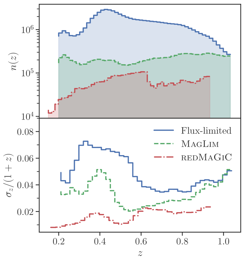
Figure 1: Galaxy counts (top panel) and mean photo-$z$ error $\sigma_{z}/(1+z)$ (bottom panel) as a function of photometric redshift for three cases of the lens samples considered in this work (see text for details).

In the rest of the paper we will derive cosmological constraints after dividing the samples in tomographic bins and using estimates for the distribution of true redshifts per bin.

The estimate for galaxy redshifts (photo-$z$) used for tomographic binning and galaxy selection for the MagLim and flux-limited samples is derived using the predicted value in the fitted hyper-plane from the DNF code. In turn, it has been shown that the stacking of the nearest-neighbor redshift allows the method to replicate science sample redshift distributions accurately [54, 55], and results and performance in Y3 GOLD are similar to those found previously by [56]. In follow-up papers we will investigate the performance of this approach for MagLim against direct calibration with spectroscopic fields [32] and clustering redshifts [57] in more detail. Hence for the estimates of the redshift distribution of galaxies in each tomographic bin, $n(z)$, we use the stacking of the nearest-neighbor redshifts of the galaxies in the sample.

For the redMaGiC sample we assume that the redshift probability distribution function (PDF) for each galaxy is a Gaussian distribution with mean given by the redMaGiC best-fit redshift and standard deviation $\sigma_{z}$. We then obtain an overall estimate of the redshift distributions by stacking these Gaussian PDFs [1, 53].

II.4 Survey area and angular mask

The footprint of the DES Y3 GOLD catalog amounts to 4946 ${\rm deg}^{2}$. For cosmology analyses, additional masking is applied to remove bright stars and other foreground objects, and also regions of the footprint that have some deficiency in the source extraction of photometric measurement (a.k.a. bad regions). As a result, the effective area is reduced by 659.68 ${\rm deg}^{2}$ [34].

Then, for a given galaxy sample, we mask the regions that are too shallow in order to have a homogeneous depth across the footprint. In Figure 2 we show the fractional survey area as a function of the limiting magnitude reached in that area in the $i$-band. Samples with an overall limiting magnitude of $i=22$ or lower will be complete over $100\%$ of the footprint. If we increase the limiting magnitude to incorporate more objects into the sample, then the regions of the sky that are too shallow would need to be masked in order to achieve a homogeneous depth. Therefore, there is a trade-off between imposing limits at higher magnitudes and preserving the survey area. In Sec. IV we vary a range of limiting magnitudes in order to optimize the samples and decide not to consider those selections with $i>22.75$, at which point we would need to mask $\sim 10\%$ or more of the sky area.

The samples that we find to be optimal in terms of 2$\times$2pt cosmological constraints are complete in regions of the survey deeper than $i=22.2$ magnitudes. Therefore, we will consider such regions as our baseline footprint. This implies masking out about $\sim 1\%$ of the area. A similar masking is applied for the redMaGiC sample. We use depth information from the redMaGiC catalogs to mask out the regions in the footprint that are too shallow. Since we want to compare the cosmological constraints obtained from the optimal samples with the redMaGiC sample, we then combine these two masks resulting in a unique mask that is applied to both. Using the same mask for both samples reduces the area by an additional $\sim 100$ ${\rm deg}^{2}$, yielding a final effective area of $4182$ ${\rm deg}^{2}$. For simplicity, we use the same mask for all sample selections. We note that this is optimistic for those samples in Sec. IV with limiting magnitudes larger than 22.2.

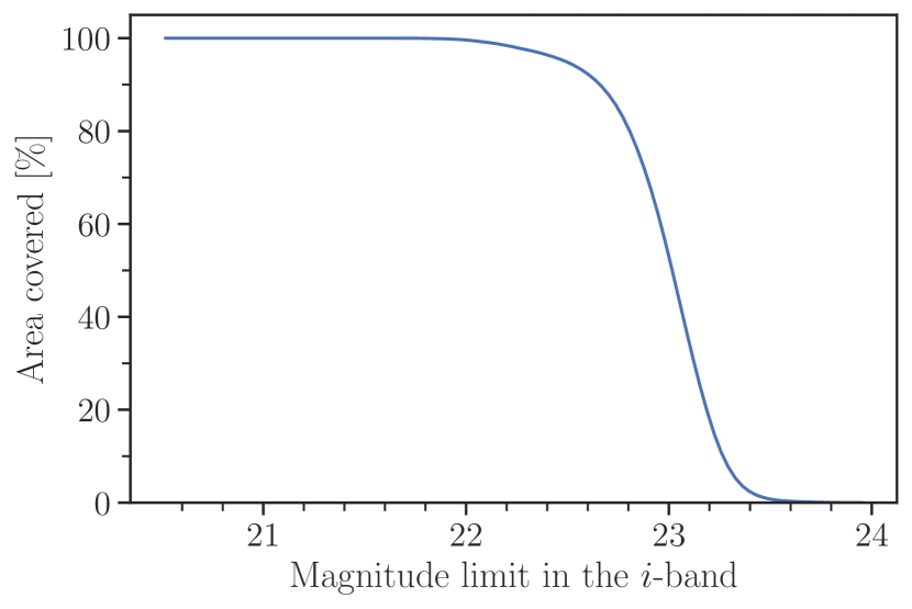
Figure 2: Percentage of survey area as a function of the limiting magnitude in the $i$-band. The reference full area includes all the baseline quality cuts corresponding to the DES Y3 GOLD dataset.

III Forecasting Methodology

In what follows, we describe the methodology employed for sample optimization. For each magnitude cut considered we access the catalog and apply the sample selection, which leads to a given number density and redshift distribution per tomographic bin. From these, we produce theory data-vectors and covariances that are subsequently used to derive cosmological parameter constraints following the forecasting methodology that we present next.

III.1 Likelihood exploration

In order to investigate the potential gains in cosmological constraints, we run simulated likelihood analyses with Fisher matrix [58, 59] and MCMC methods. The Fisher matrix is commonly used for forecasting constraints because it is fast to compute and provides an approximation for the covariance matrix of the parameters. However, since the Fisher matrix is a local approximation of the likelihood, it can provide inaccurate results for non-Gaussian posterior distributions, as is the case when there are degeneracies between parameters (see e.g. [60]). A more robust approach for forecasting is possible by sampling the full posterior distributions using an MCMC approach.

We sample the posterior in the $n$-dimensional parameter space by computing the likelihood at every step, where $n$ is the number of parameters ($\vec{p}$) we vary in our analysis (see Table 1). We assume the likelihood to be Gaussian,

$$\begin{gathered}\ln\mathcal{L}(\vec{d}|\vec{m}(\vec{p}))=\\ -\frac{1}{2}\sum^{N}_{ij}\left(d_{i}-m_{i}(\vec{p})\right)C^{-1}_{ij}\left(d_{j}-m_{j}(\vec{p})\right).\end{gathered}$$ (1)

Here $N$ is the number of data points, $\vec{m}(\vec{p})$ are the theoretical predictions as a function of the parameters we allow to vary, $\vec{d}$ is the noiseless theory data vector (the set of theoretical predictions evaluated at the fiducial cosmology), and $C$ is the covariance matrix, also evaluated at the fiducial cosmology (see Table 1). The posterior distribution of the parameters is given by:

$$P(\vec{m}(\vec{p})|\vec{d})\propto\mathcal{L}(\vec{d}|\vec{m}(\vec{p}))P_{\rm prior}(\vec{p}),$$ (2)

where $P_{\rm prior}(\vec{p})$ is the prior on the parameters. The Fisher matrix is defined as the expectation value of the curvature of the log-likelihood evaluated at the maximum likelihood point, i.e. the fiducial values of the parameters $\vec{p}_{0}$

$$F_{ij}\equiv-\left\langle\left.\dfrac{\partial^{2}\log\mathcal{L}}{\partial p_{i}\partial p_{j}}\right|_{\vec{p}=\vec{p}_{0}}\right\rangle.$$ (3)

We can include Gaussian priors by adding a prior matrix

$$F_{ij}^{P}=\delta_{ij}\dfrac{1}{(\sigma_{i}^{P})^{2}},$$ (4)

where $\sigma_{i}^{P}$ is the standard deviation on the parameter $p_{i}$ assumed as a prior. According to the Cramér-Rao inequality, the Fisher matrix gives a lower bound on the error $\sigma$ on a parameter $p_{i}$,

$$\sigma(p_{i})\geq\sqrt{(F^{-1})_{ii}}.$$ (5)

A commonly used metric to measure the constraining power of a given data set is the figure of merit (FoM). The FoM for a subset of cosmological parameters $p$ is defined as

$$\mathrm{FoM}_{p}=\dfrac{1}{\sqrt{\det\left[(F^{-1})_{p}\right]}},$$ (6)

where $(F^{-1})_{p}$ is the selection on $(F^{-1})$ of the rows and columns corresponding to the subset of parameters $p$. An intuitive way to understand the FoM is to consider a subset of two parameters. In that case, the FoM is inversely proportional to the area of the confidence ellipse of these two parameters.

One of the most important factors for the reliability of a Fisher matrix is the stability of the numerical derivatives (see e.g. [60, 61, 62]). The computation of the derivatives involves evaluating the likelihood at several points in the vicinity of the fiducial values of the parameters, assuming a given step size. The problem is that if the step size is too large, the numerical derivative may not be accurate. On the other hand, if the step size is too small, the derivative estimate will be unreliable due to numerical instabilities. For this purpose, when computing a Fisher matrix, we iteratively vary the step size for each parameter until we reach a certain tolerance. In the following, we explain the details of this process. We first compute the derivatives at an initial step size of 0.01 (1%) in units of the range of each parameter. Assuming a maximum step size $s_{\max}=0.05$ (which is a reasonable boundary according to [63]), in each iteration we vary the step sizes to the minimum value between $s_{\max}$ and the predicted $\sigma$ error on that parameter: $s_{\mathrm{new}}=\min(s_{\max},\,\sigma(p_{i}))$. The algorithm converges when the differences in the sigma errors $\sigma(p_{i})$ are below a tolerance of 0.01 and the differences in the predicted covariance matrix of the parameters are below $10^{-4}$.

Another important factor is the treatment of priors in the Fisher matrix estimation. In general, when analyzing data we assume wide flat priors for the cosmological parameters in order to avoid having cosmological results that depend on the priors assumed. However, as mentioned before, the Fisher matrix will fail to estimate the posterior distributions in the presence of non-Gaussianities, which can lead to confidence contours that extend beyond the physically meaningful parameter range. In order to address this, we apply wide Gaussian priors for the parameters listed with flat priors in Table 1, assuming in Eq. (4) a standard deviation equal to half the limits $[a,b]$ of the parameter range in Table 1: $\sigma_{i}^{P}=(b-a)/2$. This was the approach taken in [61], which resulted in a good agreement between Fisher and MCMC. In the case of nuisance parameters with Gaussian priors, we just assume as $\sigma_{i}^{P}$ the $\sigma$ values listed in Table 1.

Even though we have taken measures to ensure our Fisher matrices are reliable, the predicted constraints $\sigma(p_{i})$ will still have an uncertainty of order $10\%$ with respect to other Fisher codes and MCMC methods [62, 61, 63]. For this reason, in Sec. V.2 we compare a representative set of our Fisher forecasts against the constraints coming from a full MCMC sampling of the posterior. Nevertheless, we rely on the Fisher matrix for most of our forecasts, with the exception of Sec. V.2, in which we show the MCMC constraints for redMaGiC and the optimal samples.

In this paper we use CosmoSIS [64] to compute the Fisher matrices. For the MCMC simulated likelihood analyses, we sample the posterior distribution using the Multinest [65] wrapper in CosmoSIS.

III.2 Theory Modelling

In this section, we describe the model we use to characterize galaxy clustering and galaxy-galaxy lensing and their covariance matrix. As seen in Sec. III.1, we use these to extract cosmological information from a given data vector that, in our case, is a noiseless theoretical prediction at the fiducial cosmology. The model depends upon both cosmological parameters and astrophysical and systematic nuisance parameters (see Sec. III.3). In Appendix A, we validate the numerical implementation of our covariances by comparing the constraints coming from two different covariance codes.

III.2.1 Observables

The observables we consider in the simulated likelihood analyses are the galaxy clustering and galaxy-galaxy lensing two-point angular correlation functions, i.e. the correlations in the positions of the lens galaxies, and the correlation between these positions and the source galaxy shears.

Under the Limber approximation [66], we can construct their respective angular power spectra as a function of multipole $\ell$ in the following way,

$$\begin{gathered}C^{ij}_{\delta_{g}\delta_{g}}(\ell)=\int d\chi\frac{q_{\delta_{\rm g}}^{i}\left(\frac{\ell+\frac{1}{2}}{\chi},\chi\right)\,q_{\delta_{\rm g}}^{j}\left(\frac{\ell+\frac{1}{2}}{\chi},\chi\right)}{\chi^{2}}\,\\ \times\,P_{\rm NL}\left(\frac{\ell+\frac{1}{2}}{\chi},z(\chi)\right),\end{gathered}$$ (7)

$$\begin{gathered}C^{ij}_{\delta_{g}\kappa}(\ell)=\int d\chi\frac{q_{\delta_{\rm g}}^{i}\left(\frac{\ell+\frac{1}{2}}{\chi},\chi\right)\,q_{\kappa}^{j}(\chi)}{\chi^{2}}\,\\ \times\,P_{\rm NL}\left(\frac{\ell+\frac{1}{2}}{\chi},z(\chi)\right),\end{gathered}$$ (8)

where $P_{\rm NL}(k,z)$ is the non-linear matter power spectrum, and $q_{\delta_{\rm g}}^{i}$ and $q^{j}_{\kappa}$ are respectively the density kernel in the redshift bin $i$ from the lens sample, and the lensing efficiency in the redshift bin $j$ from the source sample. These kernels depend, respectively, on the redshift distributions of lens ($n^{i}_{\delta_{g}}(z)$) and source ($n^{i}_{\kappa}(z)$) galaxy samples normalized by their respective total number densities in that redshift bin ($\bar{n}^{i}_{\delta_{g}}$ for the lenses and $\bar{n}^{i}_{\kappa}$ for the sources), and can be expressed as a function of the comoving distance $\chi$ in the following way,

$$q_{\delta_{\rm g}}^{i}(k,\,\chi)=b^{i}(k,z(\chi))\,\frac{n_{\delta_{g}}^{i}(z(\chi))}{\bar{n}_{\rm g}^{i}}\,\frac{dz}{d\chi},$$ (9)

$$\begin{gathered}q_{\kappa}^{i}(\chi)=\frac{3H_{0}^{2}\Omega_{\rm m}}{2c^{2}}\,\frac{\chi}{a(\chi)}\,\\ \times\,\int_{\chi}^{\chi_{\rm h}}\mathrm{d}\chi^{\prime}\frac{n_{\kappa}^{i}(z(\chi^{\prime}))\mathrm{d}z/\mathrm{d}\chi^{\prime}}{\bar{n}_{\kappa}^{i}}\frac{\chi^{\prime}-\chi}{\chi^{\prime}}\,,\end{gathered}$$ (10)

where $H_{0}$ is the Hubble constant, $c$ is the speed of light, $a$ is the scale factor, and $b^{i}(k,z)$ is the galaxy bias, a nuisance parameter that we vary in our analysis (see Sec. III.3). We adopt a linear galaxy bias model (independent of the scale $k$), with a single galaxy bias $b_{i}$ parameter for each redshift bin.

Under the flat-sky approximation, the galaxy clustering and galaxy-galaxy lensing angular two-point correlation functions can be computed from the angular power spectra from Eqs. (7) and (8) in the following way,

$$w^{ij}(\theta)=\int\dfrac{\mathrm{d}\ell\,\ell}{2\pi}J_{0}(\ell\theta)C^{ij}_{\delta_{g}\delta_{g}}(\ell),$$ (11)

$$\begin{gathered}\gamma_{\rm t}^{ij}(\theta)=(1+m^{j})\int\dfrac{\mathrm{d}\ell\,\ell}{2\pi}J_{2}(\ell\theta)C^{ij}_{\delta_{g}\kappa}(\ell),\end{gathered}$$ (12)

where $J_{n}$ is the $n$-th order Bessel function of the first kind, and $m^{j}$ is the multiplicative shear bias, a nuisance parameter introduced to take into consideration potential biases in the inferred shear.

In most of this work we restrict $w(\theta)$ to auto-correlations within each redshift bin, i.e. we just consider $w^{ii}$. However, in Sec. VI.1 we test the impact of including galaxy clustering cross-correlations between redshift bins in our analysis.

In addition to the galaxy shear induced by gravitational lensing, galaxy shapes can also be intrinsically aligned as a result of their formation and evolution in the same large-scale structure environment. The impact of intrinsic alignments (IA) can be modeled using a power spectrum shape and an amplitude $A(z)$. We assume the non-linear alignment model (NLA) [67, 68] for the IA power spectrum, which impacts the lensing efficiency in the following way,

$$q_{\kappa}^{i}(\chi)\rightarrow q_{\kappa}^{i}(\chi)-A(z(\chi))\dfrac{n_{\kappa}^{i}(z(\chi))}{\bar{n}_{\kappa}^{i}}\dfrac{\mathrm{d}z}{\mathrm{d}\chi}.$$ (13)

We model the IA amplitude assuming a power-law scaling with redshift,

$$A(z)=A_{\mathrm{IA},0}\left(\dfrac{1+z}{1+z_{0}}\right)^{\alpha_{\mathrm{IA}}}\dfrac{C_{1}\rho_{\textrm{crit}}}{D(z)},$$ (14)

where $D(z)$ is the linear growth factor. The pivot redshift is chosen to be approximately the mean redshift of the sources, $z_{0}=0.62$, and $C_{1}\rho_{\textrm{crit}}=0.0134$ is a normalization derived from SuperCOSMOS observations [68]. Therefore, the IA model assumed adds two extra nuisance parameters in our analysis: $A_{\mathrm{IA},0}$ and $\alpha_{\mathrm{IA}}$.

We note that magnification, which we do not include in our modeling, will be significant when using flux-limited samples on a real data analysis. Ref. [69, in prep.] will show the measurement and validation of the magnification coefficients for both redMaGiC and the optimal sample resulting from this work. These coefficients will be included in the DES Y3 analysis to avoid biases on the cosmological constraints. However, the constraining power is only slightly degraded when marginalizing over the magnification coefficients [69]. Therefore, our conclusions are not affected by the neglect of magnification effects.

We calculate the power spectrum using the Boltzmann code CAMB [70, 71] with the Halofit extension to nonlinear scales [72, 73] and the neutrino extension from [74]. We use CosmoSIS to compute the galaxy clustering and tangential shear two-point functions.

III.2.2 Covariance

Following the notation in Refs. [75, 76], in the flat sky limit, the real space covariance of two angular two-point functions $\Xi,\,\Theta\in\{w,\gamma_{t}\}$ at angles $\theta$ and $\theta^{\prime}$ is related to the covariance of the angular power spectra by

$$\begin{gathered}\mathrm{Cov}(\Xi^{ij}(\theta),\,\Theta^{km}(\theta^{\prime}))=\\ \frac{1}{4\pi^{2}}\int\mathrm{d}\ell\,\ell J_{n(\Xi)}(\ell\theta)\int\mathrm{d}\ell^{\prime}J_{n(\Theta)}(\ell^{\prime}\theta^{\prime})\\ \times\left[\mathrm{Cov}^{G}(C_{\Xi}^{ij}(\ell),C_{\Theta}^{km}(\ell^{\prime}))+\mathrm{Cov}^{NG}(C_{\Xi}^{ij}(\ell),C_{\Theta}^{km}(\ell^{\prime}))\right],\end{gathered}$$ (15)

with $C_{\gamma_{t}}\equiv C_{\delta_{g}\kappa}$ from Eq. (8), and $C_{w}\equiv C_{\delta_{g}\delta_{g}}$ from Eq. (7), and where the order of the Bessel function is $n=0$ for $w$, and $n=2$ for $\gamma_{t}$. The indices $i,j,k,m$ denote the redshift bins. All two-point functions are evaluated in 20 log-spaced angular bins over the range $2.5^{\prime}<\theta<250^{\prime}$. This yields a 500$\times$500 covariance matrix if the lens sample is split in 5 tomographic bins (which is the fiducial case for the flux-limited and redMaGiC samples), and the size increases by 100 for each additional tomographic bin. The non-Gaussian covariance $\mathrm{Cov^{NG}}$ consists of a connected four-point correlation contribution [77, 78] and a super-sample contribution [79]. In the Gaussian covariance $\mathrm{Cov}^{G}$ [80] different harmonic modes $\ell$ are uncorrelated, so its harmonic transform reduces to a single integral. The Gaussian covariance has terms related to cosmic variance, shot noise ($\propto 1/\bar{n}^{i}$, with $\bar{n}^{i}$ being the mean number density in each tomographic bin), and for $\gamma_{t}$ there is also shape noise coming from the ellipticity dispersion $\sigma_{\epsilon}$ [81, 82].

In general, we do not include the non-Gaussian covariance term in our analysis, as we are just interested in forecasting and comparing the cosmological constraints given by different sample definitions. In addition, we exclude small scales (see Sec. III.4), where some of the non-Gaussian terms of the covariance become dominant (the super-sample contribution also impacts large scales). We note that when comparing redMaGiC with flux-limited samples, which have much higher number density, the latter will be more impacted by non-Gaussian terms due to the reduced shot noise in the Gaussian part of the covariance. Nonetheless, we have checked that including the non-Gaussian covariance term does not impact our final MagLim gains with respect to redMaGiC after the optimization carried out in Sec. IV.1.

We use two different codes to compute the Gaussian covariance: CosmoSIS [64] and CosmoLike [83], which was validated against simulations in [75]. In Appendix A we check that our results are the same independently of the code we use to compute the covariances.

III.3 Parameter space and priors

The cosmological model we consider in this work is spatially flat $w$CDM (i.e. having a free parameter for the dark energy equation of state) with fixed neutrino mass corresponding to the minimum allowed neutrino mass of 0.06 eV from oscillation experiments [84]. We split the neutrino mass equally among the three eigenstates, to be consistent with [12].

Table 1: The fiducial parameter values and priors for cosmological and nuisance parameters used in this analysis. Square brackets denote a flat prior over the indicated range, while parentheses denote a Gaussian prior of the form $\mathcal{N}(\mu,\sigma)$.

Parameter	Fiducial	Prior
Cosmology
$\Omega_{\rm m}$	0.2837	[0.1, 0.9]
$A_{\mathrm{s}}/10^{-9}$	2.2606	[$0.5$, $5.0$]
$n_{\rm s}$	0.9686	[0.87, 1.07]
$w$	-1.0	[-2, -0.33]
$\Omega_{\rm b}$	0.062	[0.03, 0.07]
$h_{0}$	0.8433	[0.55, 0.9]
$\Omega_{\nu}h^{2}$	$6.155\times 10^{-4}$	Fixed
$\Omega_{\mathrm{K}}$	0	Fixed
$\tau$	0.08	Fixed
Galaxy bias (redMaGiC)
$b^{i}$	$1.4,1.6,1.6,1.93,1.99$	[0.8,3.0]
Galaxy bias (MagLim)
$b^{i}$	$1.49,1.86,1.81,1.90,2.26,2.33$	[0.8,3.0]
Galaxy bias (Flux-limited)
$b^{i}$	$1.07,1.24,1.34,1.56,1.96$	[0.8,3.0]
Intrinsic alignment
$A_{\mathrm{IA}}$	0.0	[-5.0,5.0]
$\alpha_{\mathrm{IA}}$	0.0	[-5.0,5.0]
Lens photo-z shift (redMaGiC)
$\Delta z_{{\rm l}}^{1}$	0.0	(0.0,0.0035)
$\Delta z_{{\rm l}}^{2}$	0.0	(0.0,0.0035)
$\Delta z_{{\rm l}}^{3}$	0.0	(0.0,0.003)
$\Delta z_{{\rm l}}^{4}$	0.0	(0.0,0.005)
$\Delta z_{{\rm l}}^{5}$	0.0	(0.0,0.005)
Lens photo-z shift (MagLim)
$\Delta z_{{\rm l}}^{1}$	0.0	(0.0,0.007)
$\Delta z_{{\rm l}}^{2}$	0.0	(0.0,0.007)
$\Delta z_{{\rm l}}^{3}$	0.0	(0.0,0.006)
$\Delta z_{{\rm l}}^{4}$	0.0	(0.0,0.01)
$\Delta z_{{\rm l}}^{5}$	0.0	(0.0,0.01)
$\Delta z_{{\rm l}}^{6}$	0.0	(0.0,0.01)
Lens photo-z shift (Flux-limited)
$\Delta z_{{\rm l}}^{1}$	0.0	(0.0,0.014)
$\Delta z_{{\rm l}}^{2}$	0.0	(0.0,0.014)
$\Delta z_{{\rm l}}^{3}$	0.0	(0.0,0.012)
$\Delta z_{{\rm l}}^{4}$	0.0	(0.0,0.02)
$\Delta z_{{\rm l}}^{5}$	0.0	(0.0,0.02)
Source photo-z shift
$\Delta z_{{\rm s}}^{1}$	0.002	(0.0,0.016)
$\Delta z_{{\rm s}}^{2}$	-0.015	(0.0,0.013)
$\Delta z_{{\rm s}}^{3}$	0.007	(0.0,0.011)
$\Delta z_{{\rm s}}^{4}$	-0.018	(0.0,0.022)
Shear calibration
$m^{i}\,(i=1,4)$	0.012	(0.012, 0.023)

The fiducial cosmological parameter values correspond to the best-fits of the posterior distributions from the DES Y1 $\Lambda$CDM  analysis in [12] which obtained cosmological constraints from the combination of galaxy clustering, galaxy-galaxy lensing, and cosmic shear (a.k.a. 3$\times$2pt).

We bin the samples described in Sec. II.1 in several tomographic bins. For the MagLim sample we split the selection in 6 redshift bins from $z=0.2$ to $z=1.05$, with a width of $\Delta z=0.15$. We consider the same $z$ range for the flux-limited sample, but in that case we split the selection in 5 $z$ bins with balanced number density across the bins. For redMaGiC we split the sample in 5 $z$ bins from $z=0.15$ to $z=0.95$, similarly to DES Y1 [53]. See Table 2 for the $z$ ranges in each tomographic bin of the samples. We keep fixed this fiducial redshift binning throughout this work, except for Sec. VI.1 in which we consider alternative tomographic binnings.

For the sources we use the Metacalibration sample from the DES Y1 cosmic shear analysis [39], which is divided in 4 tomographic bins: $0.2<z<0.43$, $0.43<z<0.63$, $0.63<z<0.9$, and $0.9<z<1.3$. See Figure 3 for the normalized redshift distributions.

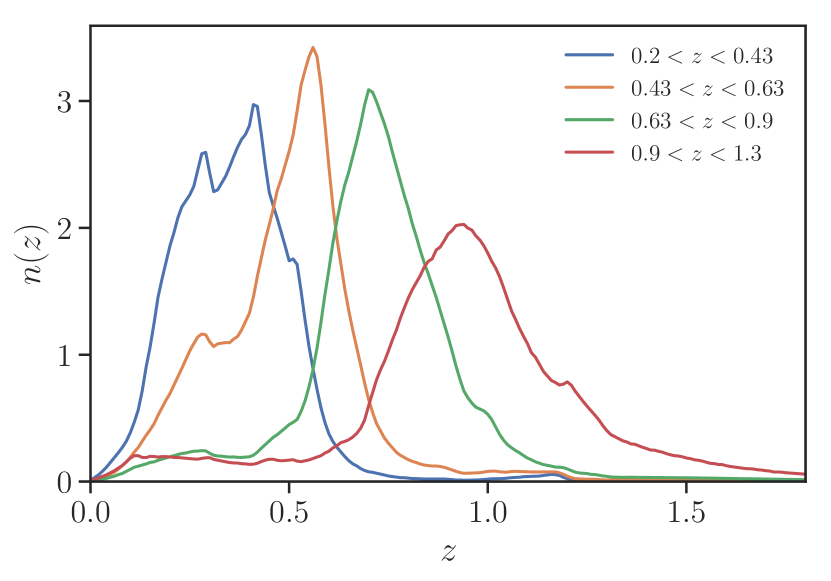
Figure 3: Normalized redshift distributions for the sources, corresponding to DES Y1 Metacalibration galaxies.

In addition to the 6 cosmological parameters, our model contains about 20 nuisance parameters (22 for MagLim due to the extra redshift bin). These are the galaxy bias parameters for the lens samples (one $b^{i}$ per redshift bin), the multiplicative shear biases (one $m^{i}$ parameter for each source redshift bin), two parameters related to the intrinsic alignment model, $A_{\mathrm{IA}}$ and $\eta_{\mathrm{IA}}$, and the photo-z shift parameters for each redshift bin of the lenses and the sources, $\Delta z^{i}$.

These shift parameters are used in our analysis to quantify uncertainties in the redshift distribution. We assume that the true redshift distribution $n^{i}(z)$ in bin $i$ is a shifted version of the photometrically derived distribution:

$$n^{i}(z)=n^{i}_{\mathrm{PZ}}(z-\Delta z^{i}).$$ (16)

The fiducial values and priors assumed for these parameters, shown in Table 1, are consistent with the DES Y1 3$\times$2 analysis [12], except that the lens photo-z shifts are treated as described below. For the MagLim sample, we assume fiducial values for the galaxy bias based on galaxy clustering measurements on a 10% subsample of the data, in consistency with the Y3 blinding scheme [85].

For the flux-limited sample we assume fiducial galaxy bias values based on the galaxy clustering measurements from DES Science Verification (SV) data [29], where a similar flux-limited sample was defined. In Sec. VI.2 we check that our conclusions in this work are basically insensitive to changes in the fiducial galaxy bias values.

For the photo-$z$ shift parameters we assume the same priors as in DES Y1 for the sources, since we are using the same redshift distributions. For the lenses, in the DES Y1 data analysis the shift values and their associated errors were obtained by re-calibrating the mean of the baseline redshift distributions to match those from a clustering-redshift method, given a reference spectroscopic sample. In DES Y1 this sample was made of $\sim 20,000$ CMASS and LOWZ galaxies in $\sim$ 124 ${\rm deg}^{2}$ area overlap with SDSS DR12 [86]. For the Y3 analysis the DES footprint overlaps over a much larger area with SDSS DR12 in addition to eBOSS, which increases the reference sample by about a factor of ten in number of galaxies [57, in prep.]. Hence the associated errors $\sigma$ are found a factor of $\sim$ 2 smaller for redMaGiC than in Y1 [57]. In turn, MagLim has broader redshift distributions than redMaGiC and the errors on the shift parameters from the clustering-redshift method in Y3 are roughly twice as big than for redMaGiC. Similarly, since the flux-limited sample has even broader redshift distributions (see Figures 1 and 8), we conservatively assume priors twice as wide compared to MagLim, which is a reasonable assumption according to Y3 clustering-redshift estimates [57]. In Sec. VI.3 we test the sensitivity of our results to the assumed priors for the MagLim and flux-limited lens photo-$z$ shift parameters.

III.4 Scale cuts

At sufficiently large scales, perturbation theory can be used to calculate the matter power spectra. On smaller scales, N-body simulations are needed in order to capture the non-linear evolution of structure growth. For example, the Halofit method [72, 73], which we use in this work, employs a functional form of the matter power spectrum derived from halo models that are, in turn, calibrated from N-body simulations. However, only gravitational physics is included in these dark matter only simulations, which neglects any modification of the matter distribution due to baryonic physics processes such as star formation, radiative cooling, and feedback [87, 88, 89]. At small scales, these processes can modify the matter power spectrum significantly [90].

In order to mitigate the impact of the uncertainty in how the baryonic physics and other non-linear effects modify the matter power spectrum, we apply a set of scale cuts, which were tested in [75] for the DES Y1 analysis, such that non-linear modeling limitations (especially in the galaxy bias modeling) do not bias the cosmology results. In this work we use the same scale cuts considered for the DES Y1 baseline analysis [12], which are defined in terms of a specific comoving scale $R$,

$$\begin{gathered}R_{\delta_{g}\delta_{g}}=8\,\mathrm{Mpc}\,h^{-1},\\ R_{\delta_{g}\kappa}=12\,\mathrm{Mpc}\,h^{-1},\end{gathered}$$ (17)

where $R_{\delta_{g}\delta_{g}}$ denotes the scale cuts for the galaxy clustering data vector, and $R_{\delta_{g}\kappa}$ for galaxy-galaxy lensing. See [75] for a detailed description of how these scale cuts were determined. We then convert the comoving scale cuts into angular ones using the radial comoving distance $\chi$ to the mean of the redshift distribution in each corresponding tomographic bin $\left\langle z^{i}\right\rangle$. Thus, for redshift bin $i$ the minimum angular scale $\theta^{i}_{\min}$ included is,

$$\theta^{i}_{\min}=\dfrac{R}{\chi\,(\left\langle z^{i}\right\rangle)}.$$ (18)

IV Sample Optimization

In this section, we explore the trade-off between number density and photo-$z$ scatter by considering different flux-limited sample definitions. In particular, we define different selections for the samples described in Sec. II.1.1 and Sec. II.1.2 and see how that impacts the constraints on $w$, $\sigma_{8}$ and $\Omega_{m}$. We fix the fiducial galaxy bias, tomographic binning, and nuisance parameters as specified in Sec. III.3. The impact of fixing these is discussed in Sec. VI, in which we show that our conclusions are robust to the galaxy bias and tomographic binning assumed. We consider an area of 4580 ${\rm deg}^{2}$ for all the forecasts in this paper, even though this value is different to the final area of the data catalog, which was reduced after masking (see Sec. II.4). For each one of the galaxy selections, we only vary the photometric redshift distribution of the lens sample and its tomographic number densities. In all cases, we use the DES Y1 Metacalibration sample for the sources.

IV.1 MagLim sample

As presented in Sec. II.1.2, we consider samples in which all galaxies have a magnitude cut applied that evolves linearly with the photometric redshift estimate: $i<az_{\rm phot}+b$. In this section we consider different values of $a$ and $b$, in a range wide enough to cover a variety of number densities and $\sigma_{z}$ values.

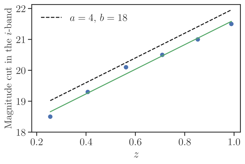
Figure 4: Different MagLim sample definitions considered. The first version (blue dots) applied a constant magnitude cut for each redshift bin, the second version (a.k.a. v0.0), in solid green, used a continuous magnitude cut evolving linearly with $z$, with slope and interception given by a fit to the blue points. In dashed black we show the final definition of the sample.

In order to get a first estimate for these values, we start by applying a different limiting magnitude in the $i$ band to each redshift bin, aiming for a number density two to three times larger than redMaGiC while keeping the photo-z scatter as low as possible. The resulting limiting magnitudes are shown in Figure 4 (blue points). We then fit the linear function to these $i$ and $z$ values obtaining $a=4.0$ and $b=17.64$. In Figure 4 we show the $i$ values used for the preliminary version of the sample, the linear fit to these values (green), hereafter v0.0, and the cut corresponding to the optimal definition of the sample (see Sec. V). In order to find the optimal sample we follow these steps:

1. Take one of the possible combinations of $(a,\ b)$ within the ranges $a=[3.5,4,4.5,5]$, $b=[17,17.5,18,18.5]$.

2. Apply the cut $i<az_{\rm phot}+b$ with the selected $a$ and $b$ values.

3. From this selection we extract the redshift distributions $n(z)$ and number densities, which will be used as input for the forecasts.

4. Generate a covariance and a theory data vector using as input for the lenses the $n(z)$ for this sample selection (and the number densities, in the case of the covariance).

5. Using this theory data vector and covariance, we run a 2$\times$2pt Fisher forecast to obtain estimated constraints and FoM on the parameters of interest (see Table 1).

As mentioned before, these ranges of $(a,\ b)$ values cover a broad variety of possible sample definitions, as the minimum values (i.e. $i<3.5z_{\rm phot}+17$) result in a sample with very few galaxies (about 75 galaxies per ${\rm deg}^{2}$), and the maximum ones (i.e. $i<5z_{\rm phot}+18.5$) result in a sample with a very large limiting magnitude ($i<23.75$), in such a way that we are practically selecting almost all the galaxies from the catalog (roughly 15300 galaxies per ${\rm deg}^{2}$). As discussed in Sec. II.4, we decide not to consider those selections that reach a limiting magnitude larger than 22.75, at which we already lose $\sim 10\%$ of the area (see Figure 2).

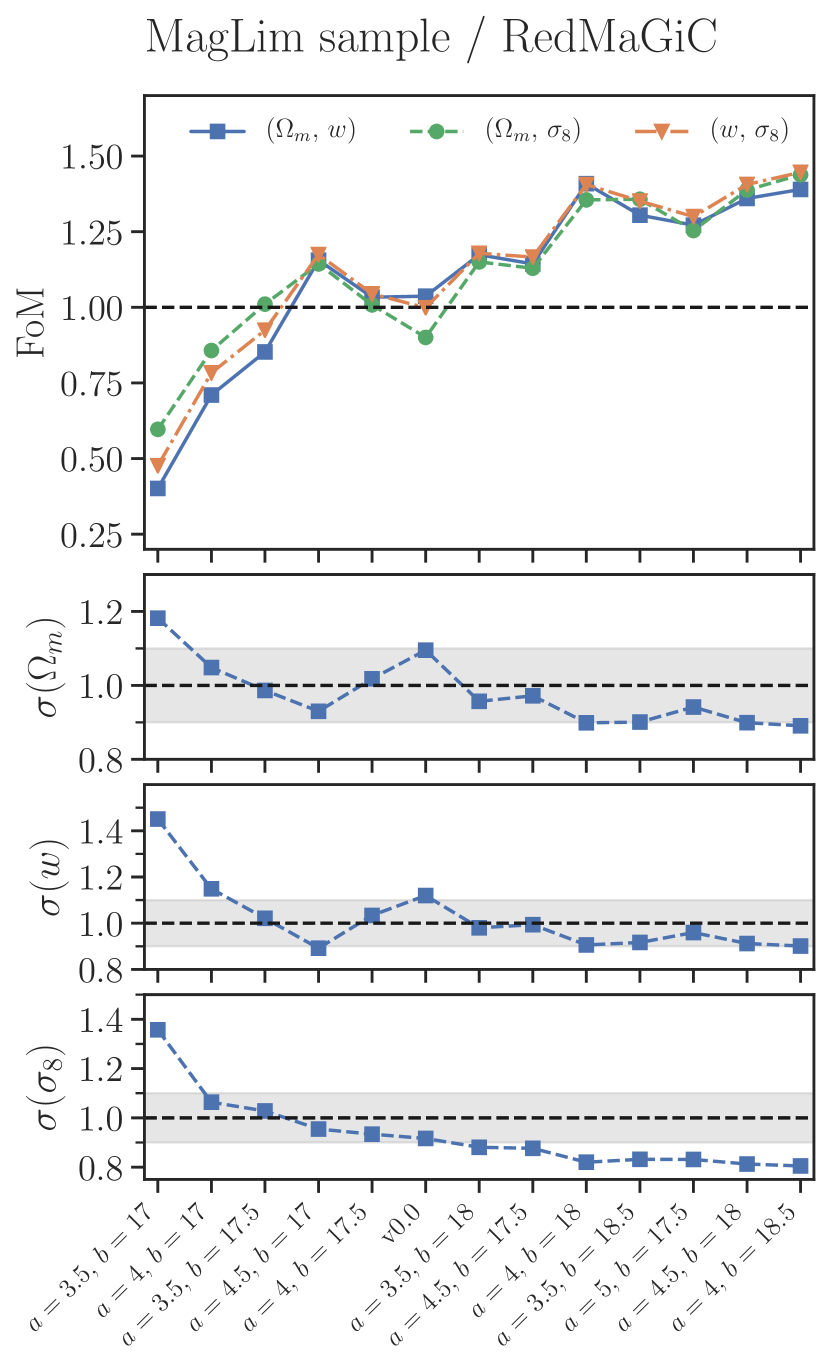
Figure 5: Standard deviations on $\Omega_{m}$, $w$ and $\sigma_{8}$ (bottom panel) and the figure of merit of their combinations in pairs (top panel) considering different magnitude limited samples (of the form $i<az_{\rm phot}+b$) normalized by estimates from the redMaGiC sample. The gray band delimits the region with $10\%$ better (lower edge) or worse (upper edge) constraints compared to redMaGiC. The samples are ordered by ascending number density (from left to right), with values ranging from $\sim 75$ to $\sim 5775$ galaxies per ${\rm deg}^{2}$.

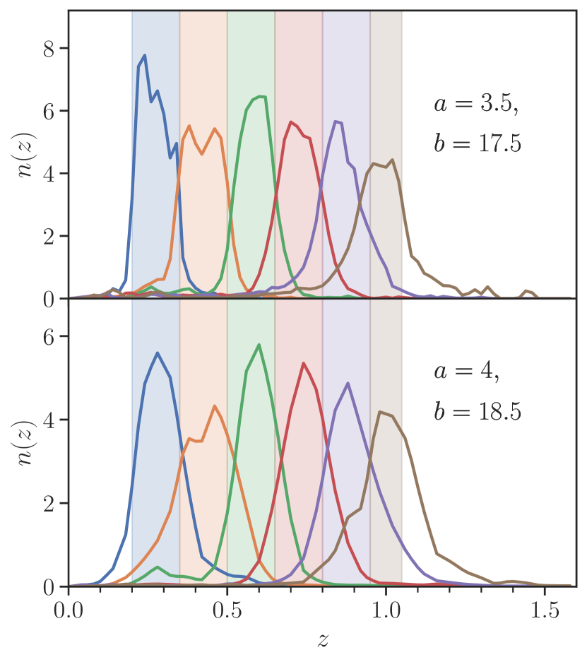
Figure 6: Normalized redshift distributions for two magnitude-limited sample selections with significantly small (top panel) and large (bottom panel) number densities (see Figure 5). The mean photo-z scatter ranges from $\sigma_{z}/(1+z)\approx 0.028$ in the top panel to $\sigma_{z}/(1+z)\approx 0.050$ in the bottom panel. The shaded bands indicate the tomographic binning assumed.

In the bottom three panels of Figure 5, we show the standard deviations resulting from the forecasts, which are normalized by the constraints obtained from the redMaGiC sample. Thus, the black dashed line represents constraints equal to those obtained from redMaGiC, while points above or below that line correspond to samples giving worse or better constraints than redMaGiC, respectively. The grey band delimits the region with 10% better or worse constraints. In the top panel we show the respective figure of merits for each pair combination of these cosmological parameters, also normalized by the FoM obtained with redMaGiC. Note that tighter constraints imply larger FoM values.

Here we see that most of the samples considered yield constraints similar or slightly better than redMaGiC. This is due to the fact that, even though the photo-z are less accurate, these samples have more galaxies and reach higher $z$ than redMaGiC (recall we consider $z_{\max}=1.05$, while for redMaGiC $z_{\max}=0.95$). One of the samples provides significantly worse constraints ($i<3.5z_{\rm phot}+17$), but this is understandable, as it corresponds to the extreme case in which very few galaxies are selected from the data catalog.

It is interesting to note that the constraints on $\sigma_{8}$ improve as the number density increases. For $\Omega_{m}$ and $w$ this trend is not so clear, in part due to the trade-off with photometric redshift accuracy which widens the redshift distributions as the number density increases. This trade-off can be seen more clearly in Figure 6, in which we compare the normalized redshift distributions of two magnitude-limited sample selections ordered by ascending number density (and, consequently, mean photo-$z$ scatter) from top to bottom. These correspond to sample selections from Figure 5 with significantly small and large number densities.

Another factor to take into account is that different combinations of $a$ and $b$ in the selection $i<az_{\rm phot}+b$ result in uneven distributions of number densities across the tomographic bins. Since we are comparing the constraints from the joint combination of galaxy clustering and galaxy-galaxy lensing, we expect to have an increased constraining power from those samples that have more galaxies at the redshifts in which the lensing efficiency kernels of the source sample peak. Thus, a sample that has more galaxies at high redshift and fewer galaxies at low redshift can provide tighter constraints than a sample with the same total number density but with the opposite distribution of galaxies.

From Figure 5 we see that the optimal sample, i.e. the one that produces the tightest constraints (higher FoM) while keeping the photo-$z$ uncertainties as low as possible, corresponds to $i<4z_{\rm phot}+18$. With a number density $2-3$ times larger than redMaGiC (see Sec. V), this sample has an increase in the FoM values of 40$\%$ (36$\%$ for the $\Omega_{m}-\sigma_{8}$ pair), providing $\sim 10-18\%$ smaller errors on the cosmological parameters.

We note that the sample with the largest number density from Figure 5, $i<4z_{\rm phot}+18.5$, provides very similar constraints to $i<4z_{\rm phot}+18$. However, this sample has larger mean photo-$z$ scatter $\sigma_{z}$ in all tomographic bins. Aside from increasing the width of the redshift distributions (see Figure 6), this could present more obstacles in the validation of the redshift distributions in a real data analysis. For this reason, the selection $i<4z_{\rm phot}+18$ is preferable.

IV.2 Flux-limited sample

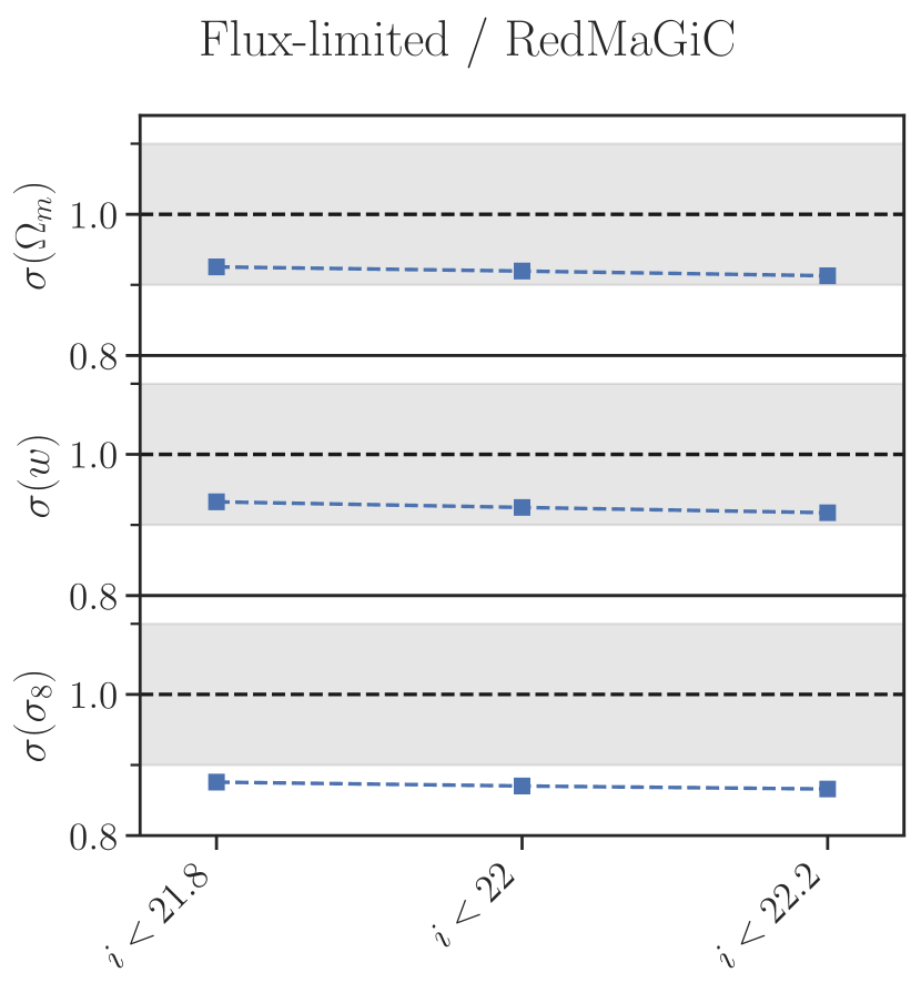
Figure 7: Standard deviations on $\Omega_{m}$, $w$ and $\sigma_{8}$ considering different definitions of the flux-limited sample, normalized by estimates from the redMaGiC sample. The gray band delimits the region with $10\%$ better (lower edge) or worse (upper edge) constraints compared to redMaGiC.

In this section we explore flux-limited samples with different limiting magnitudes in the $i$ band, as described in Sec. II.1.1. We restrict ourselves to a maximum limiting magnitude of 22.2 to avoid having to mask out a larger fraction from our total area (see Sec. II.4), this also corresponds to the limiting magnitude of the optimal MagLim sample ($i<4z_{\rm phot}+18$).

Similarly to the optimization process described for MagLim in the previous section, we run $2\times$2pt Fisher forecasts for three limiting magnitudes: [21.8, 22, 22.2]. In Figure 7 we compare the constraints obtained on $\Omega_{m}$, $w$, and $\sigma_{8}$ for each one of these flux-limited samples normalized by the redMaGiC ones. The shaded grey band delimits the region with 10% worse or better constraints compared to redMaGiC. Even though there is a significant variation in number densities in the samples considered (e.g. $i<22.2$ has twice the number density of $i<21.8$ at $0.8<z<1.05$), there is not much difference in the resulting constraints. However, we note that the scale cuts considered are conservative, and the difference in constraining power would be larger if we included smaller scales in our analysis. We find a slight improvement when increasing the number densities (going to higher limiting magnitudes). Thus, the optimal flux-limited sample is the one with limiting magnitude $i<22.2$, with which we reach  8% tighter constraints on $\Omega_{m}$ and $w$, and $13\%$ tighter on $\sigma_{8}$ with respect to redMaGiC. These improvements would be likely smaller when including shear, i.e. in the usual $3\times 2$pt analysis.

Comparing these results to those obtained for $i<4z_{\rm phot}+18$ (MagLim) we find that these constraints are somewhat worse, especially for $\sigma_{8}$. The reason for this is the trade-off between number density and photo-z scatter. The flux-limited samples have much higher number density than MagLim (see Figure 1), which in general improves the constraints because it reduces the shot noise contribution in the covariance. But at the same time, the larger $\sigma_{z}$ increases the errors on the cosmological parameters, partly due to the wider priors in the lens photo-z shift parameters $\Delta z^{i}$, and partly because the redshift distributions have larger tails and we are not including galaxy clustering cross-correlations between redshift bins. Moreover, due to the larger uncertainties in the shapes of the redshift distributions, it is not clear that a photo-$z$ shift parameter is enough to account for these uncertainties. The addition of extra nuisance parameters (e.g. a photo-$z$ width parameter for each bin) may be needed in a real data analysis, and this could degrade the constraining power of this sample. Nevertheless, we note that exploring smaller scales will be more beneficial for MagLim and, specially, for the flux-limited sample, as they are on the sample variance regime (while redMaGiC is shot noise limited).

V Optimal Samples

Table 2: Number of galaxies, mean photo-$z$ scatter, and 68% confidence width of the redshift distributions ($W_{68}$) for the optimal MagLim and flux-limited samples compared to redMaGiC, considering an effective area of 4182 ${\rm deg}^{2}$.

$z$ range	$n_{\delta_{g}}$	$\sigma_{z}/(1+z)$	$W_{68}$
redMaGiC
0.15 – 0.35	341,602	0.011	0.059
0.35 – 0.50	589,562	0.015	0.052
0.50 – 0.65	877,267	0.016	0.052
0.65 – 0.85	679,291	0.020	0.073
0.85 – 0.95	418,986	0.022	0.050
MagLim
0.20 – 0.35	1,680,160	0.034	0.064
0.35 – 0.50	1,678,655	0.043	0.082
0.50 – 0.65	1,460,354	0.022	0.061
0.65 – 0.80	1,975,242	0.027	0.069
0.80 – 0.95	2,374,205	0.034	0.077
0.95 – 1.05	1,470,893	0.044	0.097
Flux-limited
0.20 – 0.40	12,623,785	0.061	0.113
0.40 – 0.50	16,291,232	0.066	0.101
0.50 – 0.65	16,795,581	0.050	0.098
0.65 – 0.80	12,994,143	0.036	0.077
0.80 – 1.05	11,244,729	0.040	0.110

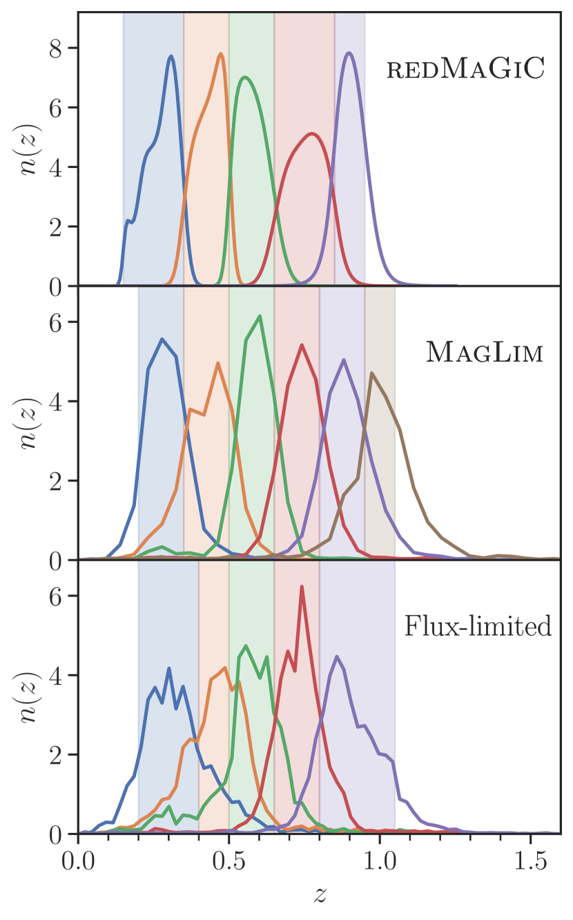
Figure 8: Normalized redshift distributions for the optimal MagLim and flux-limited samples compared to redMaGiC. The shaded bands indicate the tomographic binning of each sample.

In Sec. IV we find that the optimal sample is the MagLim sample, defined with a magnitude cut $i<4z_{\rm phot}+18$. In Table 2 we describe the fiducial tomographic binnings of the three samples, along with the number of galaxies, $n_{\delta_{g}}$, the mean photo-z scatter, $\sigma_{z}/(1+z)$, and the 68% confidence width of the redshift distributions $W_{68}$ in each redshift bin. The $W_{68}$ value is the equivalent of the standard deviation of a Gaussian distribution, and in practice is much more relevant to consider than $\sigma_{z}$ itself because it is a measure of the width of the redshift distribution, which is what enters the density kernel in the two-point functions computation (see Sec. III.2). In Figure 8 we show the redshift distributions for the three samples. The flux-limited sample is the one with larger photo-z scatter, and as a consequence, the redshift distributions are broader than with the other two samples.

In order to compare the properties of the samples under the same terms, in the following Sec. V.1 we compare the number of galaxies and $W_{68}$ values assuming the same tomographic binning. In Sec. V.2 we compare their cosmological constraints obtained from full MCMC simulated likelihood analyses.

V.1 Comparison on same tomographic binning

In this section we compare the characteristics (number density and photometric accuracy) of MagLim with the flux-limited and redMaGiC samples under the same tomographic binning. In particular, we assume the redMaGiC tomographic binning for the three samples. Since the MagLim and flux-limited samples reach a higher maximum redshift than redMaGiC, for those two samples we consider an additional redshift bin in the range $0.95<z<1.05$.

In Table 3 we show the number of galaxies and $W_{68}$ values for each redshift bin and each one of the lens samples. The MagLim sample has on average between 2 and 3 times more galaxies than redMaGiC. The difference in number density ranges from 60% more galaxies in the third bin to more than 5 times further galaxies at higher redshift ($0.85<z<0.95$), while the redshift distributions are $\sim 30\%$ wider on average for the MagLim sample.

On the other hand, the number of galaxies in the flux-limited sample is one order of magnitude larger compared to MagLim, except at high redshift ($0.85<z<1.05$) where the MagLim selection gets closer to the flux-limited selection of $i<22.2$, as they both have the same limiting magnitude at $z_{\max}=1.05$. The flux-limited sample has a high number density at the expense of larger photo-$z$ errors (see Figure 1). As a consequence, its redshift distributions are on average $~{}20\%$ wider compared to MagLim, with the difference being larger in the range $0.50<z<0.65$.

The greater number density of MagLim and flux-limited samples compared to redMaGiC is the dominant factor driving the gain of constraining power from a 2x2pt analysis. The extension to higher redshift ($z_{\max}=1.05$) is a sub-dominant effect in this case due to the weak lensing kernels peaking at $z\sim 0.6$ (see Figure 3). Therefore, the increase in number density in the other tomographic bins ($z<0.95$) dominates the overall gain of these samples compared to redMaGiC.

Table 3: Comparison of number of galaxies and 68% confidence width of the redshift distribution, $W_{68}$, for the optimal MagLim and flux-limited samples compared to redMaGiC, considering an effective area of 4182 ${\rm deg}^{2}$ and the same tomographic binning.

$z$ range	redMaGiC	MagLim	Flux-lim
	Number of galaxies
0.15 – 0.35	341,602	1,599,462	9,129,473
0.35 – 0.50	589,562	1,593,745	21,473,232
0.50 – 0.65	877,267	1,379,717	16,795,581
0.65 – 0.85	679,291	1,862,978	16,640,513
0.85 – 0.95	418,986	2,257,704	5,093,174
0.95 – 1.05		1,470,893	2,503,679
Total	2,906,708	10,164,499	71,635,652
	Width of the redshift distribution ($W_{68}$)
0.15 – 0.35	0.059	0.073	0.088
0.35 – 0.50	0.052	0.082	0.105
0.50 – 0.65	0.052	0.061	0.098
0.65 – 0.85	0.073	0.085	0.091
0.85 – 0.95	0.050	0.076	0.086
0.95 – 1.05		0.097	0.096

V.2 Cosmological constraints from MCMC likelihood analysis

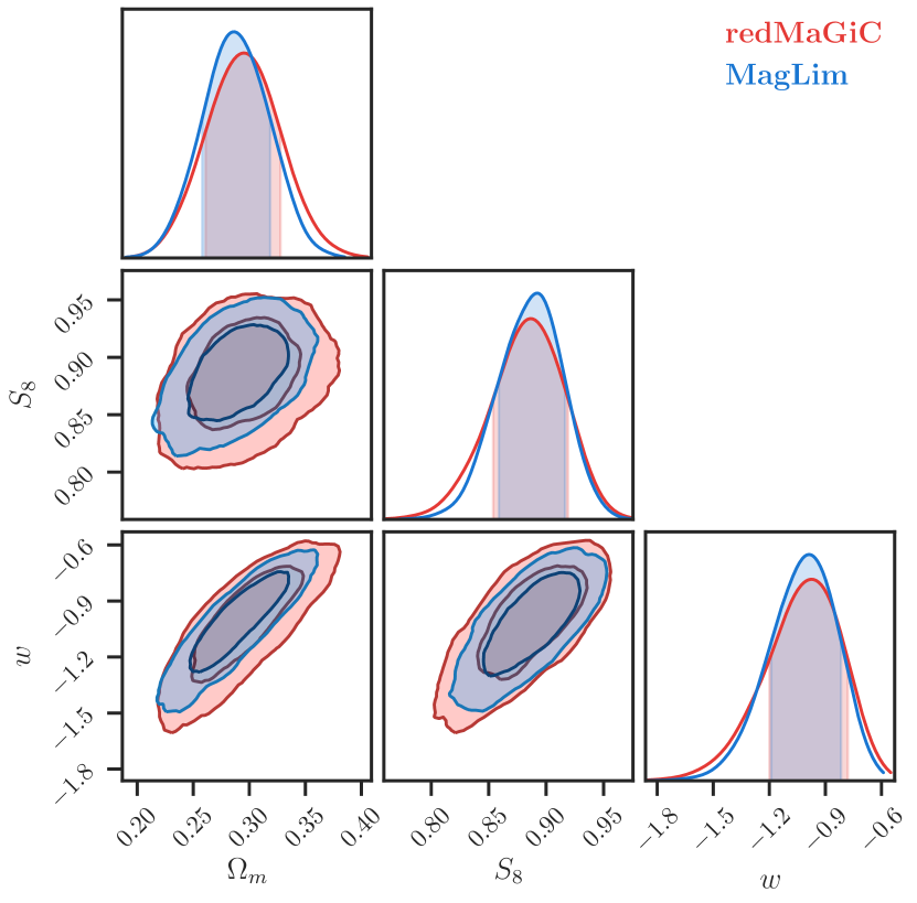
Figure 9: Comparison of 2$\times$2pt parameter constraints obtained using the DES Y3 redMaGiC (red) and MagLim (blue) samples and the DES Y1 Metacalibration source sample. Here, and in all the 2D plots below, the two sets of contours depict the 68% and 95% confidence levels (CL). The MagLim constraints are tighter by 10% on $\Omega_{m}$, 13% on $S_{8}$, and 12% on $w$ compared to redMaGiC.

In this section, we compare the cosmological constraints obtained from the optimal MagLim and flux-limited samples with respect to the redMaGiC sample after performing a full MCMC analysis of the combination of galaxy clustering and galaxy-galaxy lensing, as opposed to the Fisher matrix approach taken in the other sections. We assume the fiducial values and priors listed in Table 1 and the tomographic binnings from Table 2. However, in addition to exploring the constraints on $\sigma_{8}$, in this section we also consider the related parameter

$$S_{8}\equiv\sigma_{8}\left(\dfrac{\Omega_{m}}{0.3}\right)^{0.5},$$ (19)

since $S_{8}$ is better constrained than $\sigma_{8}$ in weak lensing surveys such as DES, and it is largely uncorrelated with $\Omega_{m}$ in the DES parameter posterior.

In Figure 9 and Table 4 we show the constraints on $\Omega_{m}$, $S_{8}$, and $w$ ($\sigma_{8}$ constraints also included in Table 4). We find that, using the MagLim sample instead of redMaGiC, we obtain 10% tighter constraints on $\Omega_{m}$, about 12-13% for $S_{8}$ and $w$, and $16\%$ on $\sigma_{8}$ . Regarding the flux-limited sample, we generally find worse constraints compared to MagLim, with the difference being 2% on $\Omega_{m}$, and 6-7% on $w$ and $\sigma_{8}$. However, when sampling the $S_{8}$ parameter, the flux-limited sample provides an 11% improvement with respect to MagLim. This is due to the flux-limited sample having a projected 2D posterior in the $S_{8}-\Omega_{m}$ plane with a slightly different inclination compared to MagLim, favoring tighter $S_{8}$ constraints.

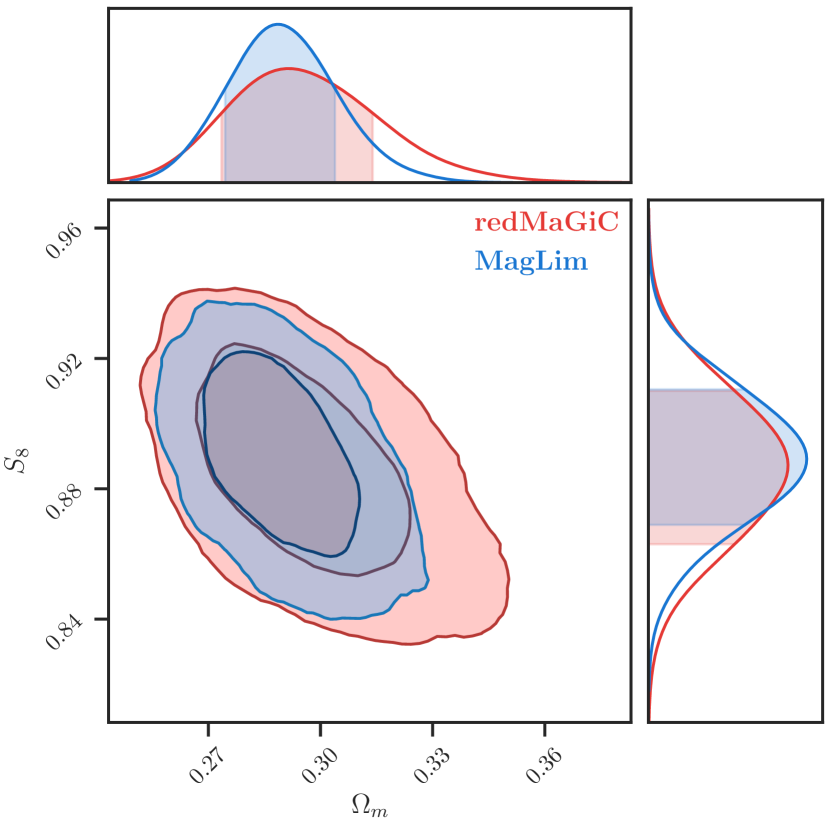
Figure 10: $\Lambda$CDM 2$\times$2pt constraints (fixing $w$) using the DES Y3 redMaGiC (red) and MagLim (blue) samples as lenses and the DES Y1 Metacalibration sample as sources. The MagLim constraints are tighter by 27% on $\Omega_{m}$, and 11% on $S_{8}$ compared to redMaGiC.

Table 4: 68% confidence level marginalized cosmological constraints in $\Lambda$CDM and wCDM for redMaGiC and the optimal MagLim and flux-limited samples.

Lens sample	$\sigma(\Omega_{m})$	$\sigma(\sigma_{8})$	$\sigma(S_{8})$	$\sigma(w)$
	$\Lambda$CDM
redMaGiC	0.019	0.043	0.022	–
MagLim	0.014	0.035	0.019	–
Flux-limited	0.017	0.037	0.018	–
	wCDM
redMaGiC	0.031	0.048	0.031	0.20
MagLim	0.028	0.040	0.027	0.18
Flux-limited	0.029	0.043	0.024	0.19

We then fix $w$ and compare the constraints on $\Omega_{m}$, $\sigma_{8}$ and $S_{8}$ assuming a $\Lambda$CDM cosmological model. In Figure 10 and Table 4 we show the constraints on these parameters from the combination of galaxy clustering and galaxy-galaxy lensing. In this case, we find a greater difference in the constraining power of the two samples. In particular, while the increase on $\sigma_{8}$ and $S_{8}$ with MagLim with respect to redMaGiC is similar (around 19% and 11%, respectively), the constraints on $\Omega_{m}$ show a $27\%$ improvement compared to redMaGiC. Thus, it seems that most of the gain in constraining power on $w$ in Figure 9 has now been absorbed by $\Omega_{m}$. Similarly to the wCDM case, the flux-limited sample yields worse constraints on $\Omega_{m}$ and $\sigma_{8}$ with respect to MagLim, with a difference of 18% and 6%, respectively, while it improves the constraints on $S_{8}$ compared to MagLim by 6% .

As discussed before, the fact we find tighter cosmological constraints with MagLim is evidently due to the greater number of galaxies (2-3 times higher) and increased depth compared to redMaGiC, reaching $z=1.05$ instead of $z=0.95$. If we included the shear 2-point correlation functions in our data vector, i.e. if we considered a 3$\times$2pt analysis, the difference between the two lens samples would be lower because the constraints would be dominated by the cosmic shear signal. However, this increase in depth of the MagLim sample would be particularly advantageous when combining the 3x2pt analysis with CMB lensing (5$\times$2pt, see [91]), as the MagLim sample will have a greater overlap with the CMB lensing kernel, providing a higher signal-to-noise ratio of galaxy clustering and CMB lensing cross-correlations.

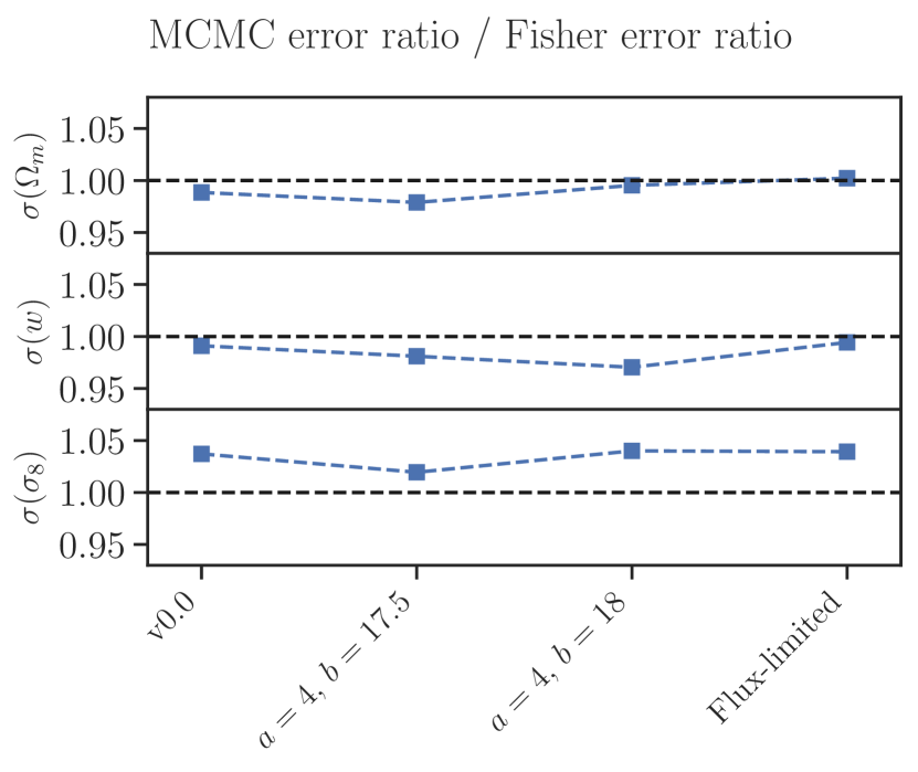
Figure 11: For each parameter $i$ and sample $j$, error ratio with respect to redMaGiC from MCMC divided by the equivalent error ratio from Fisher forecasts, i.e. $[\sigma_{j}^{i}/\sigma_{\textsc{red}}^{i}]_{\mathrm{MCMC}}/[\sigma_{j}^{i}/\sigma_{\textsc{red}}^{i}]_{\mathrm{Fisher}}$. The samples considered are the flux-limited sample and a few definitions of the MagLim sample, including the optimal one ($a=4,\,b=18$). Values larger (lower) than 1 indicate that the Fisher forecasts overestimate (underestimate) the gains of that sample with respect to redMaGiC compared to MCMC.

Now that we have MCMC constraints for the different samples, in Figure 11 we turn back to compare the gains with respect to redMaGiC with the results obtained with Fisher matrices in Sec. IV. For each parameter $i$ and sample $j$, we divide the error ratios obtained from MCMC with the error ratios using Fisher, $[\sigma_{j}^{i}/\sigma_{\textsc{red}}^{i}]_{\mathrm{MCMC}}/[\sigma_{j}^{i}/\sigma_{\textsc{red}}^{i}]_{\mathrm{Fisher}}$, where $\sigma_{\textsc{red}}$ denotes the constraints for redMaGiC. In this way we can assess the level of uncertainty in our conclusions when using Fisher matrices, despite the offset with respect to MCMC constraints due to the non-gaussianity of the posteriors. The dashed line in Figure 11 denotes perfect agreement between MCMC and Fisher in the $\sigma$ errors when normalizing by redMaGiC, while values larger (lower) than 1 indicate that Fisher overestimates (underestimates) the gains. Figure 11 shows that the difference between MCMC and Fisher error ratios is less than 5%. However, the variance of this difference across samples is small, having a scatter of $1-2\%$, in general. This is actually the level of impact in our conclusions when using Fisher, since in this paper we generally compare the gains of two different samples normalized by redMaGiC.

VI Sensitivity to Analysis Choices

VI.1 Tomographic binning and cross-correlations

In this section we test the impact of the choice of tomographic binning of the MagLim sample and the inclusion of galaxy clustering cross-correlations between redshift bins. We run $2\times 2$pt Fisher forecasts for each of the tomographic-bin cases considered and compare the constraints on $\Omega_{m}$, $\sigma_{8}$, and $w$.

Throughout this section we maintain the same global $z$ range as the fiducial sample, i.e. $0.2<z<1.05$. We first vary the edges of the tomographic binning, putting together two new configurations in which we balance the number of galaxies weighted by the galaxy bias in each redshift bin, ‘same $N_{\mathrm{gal}}\times b^{i}$’, and ‘same $N_{\mathrm{gal}}$’. The galaxy bias values we consider are listed in Table 1, and the definition of these $z$ binnings is shown in Table 5. The motivation for balancing the number of galaxies (weighted by the galaxy bias) is to have a more uniform signal-to-noise ratio across redshift, as the shot noise $\propto 1/N_{\mathrm{gal}}$ and the signal is proportional to the bias (see Eq. (9)). However, as we can see in Figure 12, where we compare the constraints coming from these different tomographic binnings, our choice of binning does not appreciably impact the 2$\times$2pt cosmological constraints.

Table 5: Different tomographic binning configurations for the MagLim sample, considering variations in the edges of the $z$ bins.

Fiducial	Same $N_{\mathrm{gal}}$	Same $N_{\mathrm{gal}}\times b^{i}$
0.20 – 0.35	0.20 – 0.36	0.20 – 0.40
0.35 – 0.50	0.36 – 0.52	0.40 – 0.55
0.50 – 0.65	0.52 – 0.69	0.55 – 0.72
0.65 – 0.80	0.69 – 0.82	0.72 – 0.85
0.80 – 0.95	0.82 – 0.93	0.85 – 0.95
0.95 – 1.05	0.93 – 1.05	0.95 – 1.05

Table 6: Different tomographic binning configurations for the MagLim sample, considering variations in the number of $z$ bins. The case with 6 $z$ bins corresponds to the fiducial tomographic binning (see e.g. Table 5).

4 $z$-bins	5 $z$-bins	7 $z$-bins	8 $z$-bins
0.20 – 0.44	0.20 – 0.40	0.20 – 0.35	0.20 – 0.31
0.44 – 0.69	0.40 – 0.60	0.35 – 0.50	0.31 – 0.44
0.69 – 0.87	0.60 – 0.77	0.50 – 0.64	0.44 – 0.57
0.87 – 1.05	0.77 – 0.90	0.64 – 0.77	0.57 – 0.69
	0.90 – 1.05	0.77 – 0.86	0.69 – 0.79
		0.86 – 0.95	0.79 – 0.87
		0.95 – 1.05	0.87 – 0.96
			0.96 – 1.05

We then vary the number of tomographic bins in which we divide the sample in the range $0.2<z<1.05$. Our fiducial tomographic binning consists of 6 $z$ bins, and we consider additionally sample selections split in 4, 5, 7, and 8 $z$ bins. See Table 6 for the details of the $z$ binning for each one of these cases. In Figure 13 we compare the estimated Fisher $2\times 2$pt constraints from each one of these sample selections with our fiducial choice of 6 $z$ bins, and we examine the importance of including galaxy clustering cross-correlations between redshift bins. The motivation for the latter is that, as seen in Figure 8, the MagLim sample has more overlap between $z$ bins than the redMaGiC sample, so galaxy clustering cross-correlations could become important for our analysis. In addition, [48] shows that the improvement on the $\Omega_{\rm m}$ and $\sigma_{8}$ constraints can be greatly increased with the number of $z$ bins and the inclusion of cross-correlations between $z$ bins, especially for samples with large overlap between bins.

We can draw several conclusions from Figure 13 (see Table 7 for a quantitative summary of the most relevant cases). First, we find that reducing the number of $z$ bins degrades the cosmological constraints. This makes sense, as reducing the number of bins while keeping fixed the total $z$ range to be covered effectively increases the width of the redshift distributions and, as shown in [92], there is a loss of information when projecting the 3D power spectrum into angular tomographic bins, with that loss being larger the wider the redshift bins. This is due to the fact that broad bins average down radial power on scales smaller than the bin width. More concretely, when splitting the sample in 4 tomographic bins instead of 6, the constraints degrade up to 13% on $\Omega_{m}$, 16% on $w$ and 11% on $\sigma_{8}$.

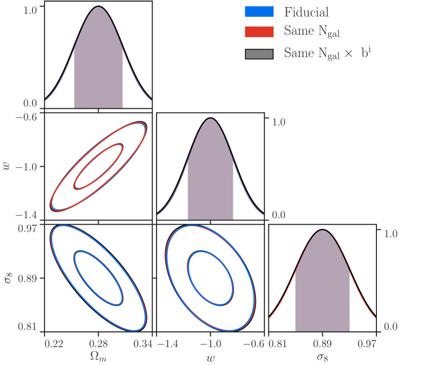
Figure 12: Comparison of 2$\times$2pt Fisher constraints considering different tomographic binnings for the DES Y3 MagLim sample, as described in Table 5. For the sources we use the DES Y1 Metacalibration sample.

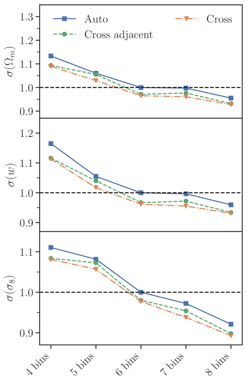
Figure 13: Comparison of 2$\times$2pt Fisher constraints considering different number of tomographic bins for the DES Y3 MagLim sample, as described in Table 6. For the sources we use the DES Y1 Metacalibration sample. All constraints are normalized by the fiducial (’auto’ with 6 redshift bins). We compare the gains obtained when only galaxy clustering auto-correlations (solid blue) are included, with the cases in which we also include cross-correlations with adjacent tomographic bins (dashed green), and when all cross- correlations among tomographic bins are included (dash-dotted orange).

Second, increasing the number of redshift bins improves the constraints, but the impact is smaller. Only when we split the sample in 8 $z$ bins do we start to find some significant improvement in all three parameters, and especially on $\sigma_{8}$. In particular, in this case the constraints improve by 4% on $\Omega_{m}$ and $w$, and 8% on $\sigma_{8}$, with respect to the fiducial. In spite of this, we keep the 6 $z$ bins tomographic binning as our fiducial, considering that splitting into a larger number of tomographic bins would require a better understanding of the tails of the redshift distributions, which is likely not captured by our treatment of photo-$z$ uncertainties (just a shift to the mean of the distribution). Another motivation for not splitting into a larger number of bins is to avoid numerical instabilities in the computation of the analytical non-Gaussian covariance. We note that the results from Figure 13 may change slightly with the inclusion of non-gaussian terms in the covariance. That is due to the non-gaussian terms being unaffected by the change in number densities in each tomographic bin, while the Gaussian part of the covariance does vary with the number densities.

Last, we study the impact of including galaxy clustering cross-correlations in our analysis. Ref. [48] shows that, for a flux-limited sample, the improvement on the cosmological constraints can be greatly increased with the number of $z$ bins and the inclusion of cross-correlations between $z$ bins. In [48] the authors consider only galaxy clustering, and fix all parameters except for $\Omega_{m}$, $\sigma_{8}$, and the photo-$z$ nuisance parameters. We have attempted to reproduce their results, and while we do not find the same level of gains on the constraints, we observe the same tendency. In Figure 13 we repeat this study for the MagLim sample, but now varying all parameters listed in Table 1, and including galaxy-galaxy lensing. We find that there is not much improvement to be gained with the inclusion of galaxy clustering cross-correlations between $z$ bins (a $3-4\%$ gain in the three cosmological parameters), and that this relative gain does not depend on the number of tomographic bins considered. We also explore the possibility of including only galaxy clustering cross-correlations with adjacent $z$ bins, which is where the overlap between bins is the largest, finding in general very similar constraints compared to when we include all cross-correlations between $z$ bins.

We also explore the potential gains on the 2$\times$2pt constraints from the flux-limited sample when including all cross-correlations between $z$ bins and splitting the sample in a larger number of bins than the fiducial (5 bins). In particular, we divide the sample in 7 tomographic bins in these redshift ranges, aiming for a balanced number density across bins: [0.2, 0.35, 0.45, 0.55, 0.65, 0.75, 0.85, 1.05]. In Figure 14 we observe that the gain on the constraints from the inclusion of cross-correlations is larger than for MagLim, as expected, since the flux-limited sample has broader redshift distributions (see Figure 8). In particular, with this sample, including cross-correlations improves the constraints by $\sim 8\%$ on $\Omega_{m}$, $\sim 11\%$ on $w$, and $\sim 4\%$ on $\sigma_{8}$. Similarly, increasing the number of tomographic bins improves the constraints by a larger amount compared to MagLim. When splitting the sample in 7 tomographic bins, the gains on the cosmological parameters with respect to the fiducial (5 bins) are of $7-8\%$ on $\Omega_{m}$ and $w$, and $12\%$ on $\sigma_{8}$. Thus, by splitting the flux-limited sample in a larger number of bins we can already obtain tighter cosmological constraints than MagLim in all three parameters. More concretely, dividing the sample in 7 tomographic bins yields constraints tighter than the fiducial MagLim (with 6 bins) by $7-8\%$.

In practice there are several complications in considering a large number of bins and in the inclusion of cross-correlations, the main ones being a much more stringent requirement for the control of the tails of the redshift distributions and a larger covariance. Moreover, as mentioned before, it is not clear that a photo-$z$ shift parameter is enough to account for these uncertainties. For these reasons, we will focus on the MagLim sample in follow-up work with DES Y3 data. Nonetheless, flux-limited samples are promising and worth exploring in future studies.

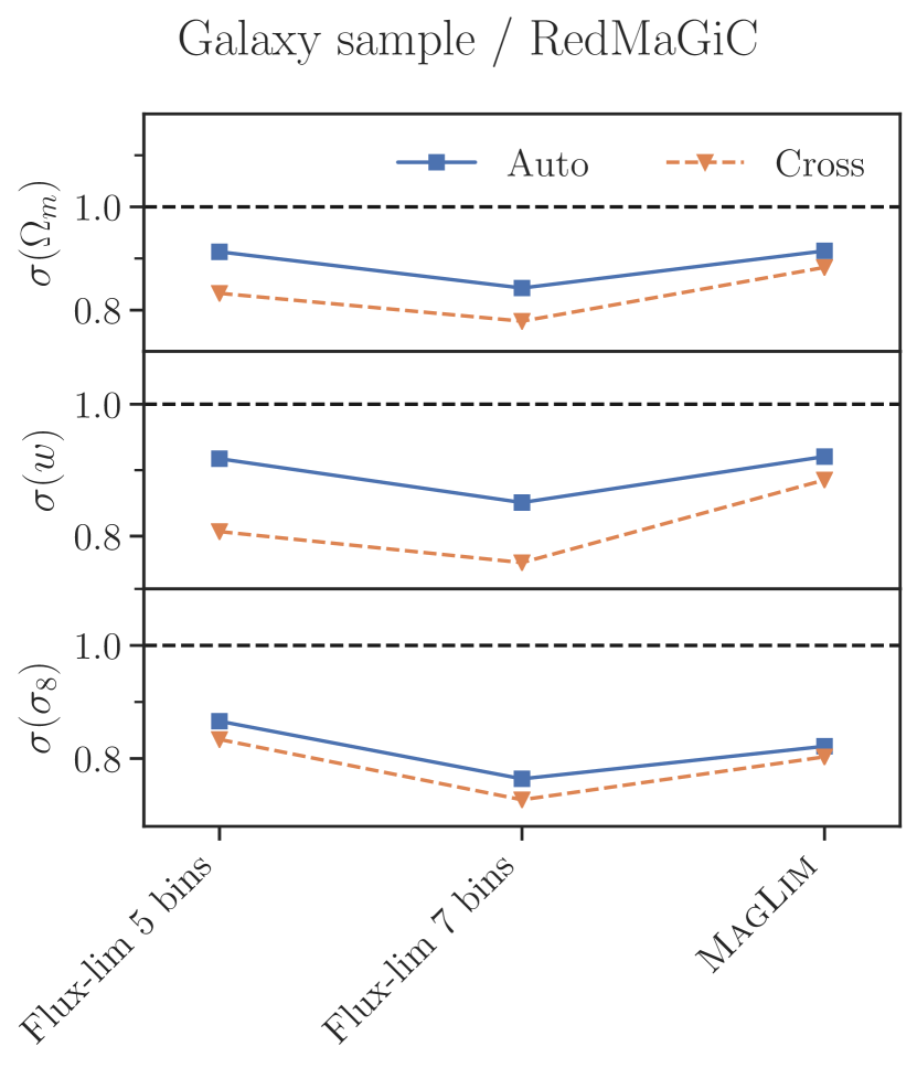
Figure 14: Comparison of 2$\times$2pt standard deviations on $\Omega_{m}$, $w$, and $\sigma_{8}$ for different numbers of tomographic bins for the flux-limited sample compared to the fiducial MagLim sample. All constraints are normalized by the redMaGiC estimates. We explore the potential gains when including all galaxy clustering cross-correlations among tomographic bins (dashed orange) with the baseline approach, i. e. including only galaxy clustering auto-correlations (solid blue). All three lens samples are built from DES Y3 data, while the sources are from the DES Y1 Metacalibration sample.

VI.2 Galaxy bias

Throughout this work we assume certain fiducial values for the galaxy bias for each one of the samples (see Table 1) to generate the theory data vectors, which we do not vary when considering different sample definitions for the MagLim and flux-limited samples in Sec. IV. In order to test the dependency of the constraints on the fiducial galaxy bias assumed, we run Fisher forecasts with completely different galaxy bias values and compare the 2$\times$2pt constraints on $\Omega_{m}$, $w$, and $\sigma_{8}$, finding almost no difference in our results. In particular, for the MagLim sample we run a forecast assuming a constant value of $2.0$ for the galaxy bias in all redshift bins, finding a difference in the constraints on the cosmological parameters of $\sim 1\%$ or less.

For the flux-limited sample, following [48] we run a forecast assuming a galaxy bias that evolves as $b(z)=1+z$, hence the galaxy bias in each redshift bin is $b^{i}=1+\bar{z}^{i}$, with $\bar{z}^{i}$ being the mean redshift in that tomographic bin. For this sample, that corresponds to $b=[1.33,1.46,1.56,1.72,1.88]$. Compared to assuming the fiducial values in Table 1, the resulting constraints on $\Omega_{m}$, $w$ and $\sigma_{8}$ differ by less than $\sim 0.5\%$. Thus the conclusions from this work do not depend on the galaxy bias assumed.

VI.3 Photometric redshift uncertainties

As described in Sec. III.3, we quantify the uncertainties in the redshift distributions by introducing a photo-$z$ shift parameter in each redshift bin, $\Delta z^{i}$, that we marginalize over in our analysis assuming a Gaussian prior with a certain $\sigma^{i}$. In this section we test the dependency of the MagLim and flux-limited sample gains on the width $\sigma$ of the prior assumed. For this purpose, we investigate a pessimistic scenario for MagLim in which the Gaussian priors on $\Delta z^{i}$ are two times wider than the fiducial in Table 1. We find that in this case the constraints degrade by $6-7\%$ for $\Omega_{m}$ and $w$, and about $3\%$ for $\sigma_{8}$.

Similarly, for the flux-limited sample we also test the impact on the constraints when increasing the width of the priors. In particular, we run a Fisher forecast with Gaussian priors three times as wide as the MagLim ones (the fiducial priors are two times wider, see Table 1). The resulting constraints are degraded by $5-8\%$ compared to the fiducial photo-$z$ prior for the flux-limited sample.

VI.4 Weak lensing systematics

In all our analyses we assume the DES Y1 source sample from [12], and its corresponding priors for the weak lensing related nuisance parameters: the shear calibration bias in each source redshift bin, $m^{i}$, the intrinsic alignment parameters ($A_{\mathrm{IA}}$, and $\alpha_{\mathrm{IA}}$), and the source photo-z shift parameters in each bin, $\Delta z_{s}^{i}$. We expect some improvement in our control of these systematics for the upcoming DES Y3 and Y6 analyses that will tighten the priors on these nuisance parameters. In this section we investigate to what extent our forecasts are limited by our (prior) knowledge of the weak lensing systematics. For this purpose we consider the ideal scenario in which we perfectly know the values of these systematic parameters, i.e. we fix them in our analysis. We find that, for the MagLim sample, we can improve the constraints up to $\sim 10\%$ for $\Omega_{m}$ and $w$, and $15\%$ for $\sigma_{8}$. The constraints on redMaGiC also improve in a similar manner, nonetheless the larger number density of MagLim could be more important in this scenario in which the weak lensing systematics are not a bottleneck. Comparing the 2$\times 2$pt constraints with fixed weak lensing systematics from MagLim and redMaGiC, we find that the relative constraining power of the former remains similar for $\Omega_{m}$ and $w$ and improves by $3\%$ for $\sigma_{8}$ with respect to what we obtain for the two samples when marginalizing the weak lensing nuisance parameters.

The gain in constraining power that the MagLim sample offers compared to redMaGiC is mainly due to the larger number density, as that reduces the shot noise contribution in the covariance. We also explore in this section how much are we limited by the shot noise of the lens sample. We compute a covariance matrix setting the galaxy clustering shot noise contribution to zero (equivalent to assuming a practically infinite number density), and we find for the MagLim sample an improvement of $6\%$ for $\Omega_{m}$, $3\%$ for $w$, and $12\%$ for $\sigma_{8}$ with respect to the fiducial case. Therefore, the MagLim sample is relatively close to the limit without shot noise.

Table 7: Percentage gains in the $\Omega_{m}$, $\sigma_{8}$ and $w$ standard deviations with respect to the fiducial for MagLim, considering the most relevant alternative analysis choices discussed in Sec. VI. Negative values indicate a decrease in the constraining power compared to the fiducial.

	$\sigma(\Omega_{m})$	$\sigma(\sigma_{8})$	$\sigma(w)$
auto $+$ cross	3.5%	2.3%	3.8%
4 tomographic bins	-13.3%	-11.1%	-16.5%
8 tomographic bins	4.5%	7.9%	4.0%
x2 photo-z shift priors	-6.3%	-3.0%	-6.6%
fixed WL systematics	9.8%	15.1%	9.4%
infinite number density	5.7%	11.8%	2.8%

VII Conclusions

In this work we define an optimized lens sample for DES Y3 that serves as an alternative to redMaGiC for cosmological analyses involving galaxy clustering measurements. Assuming the DES Y1 Metacalibration sample for the sources, we compare the cosmological constraints on $\Omega_{m}$, $\sigma_{8}$ and $w$ from the joint analysis of galaxy clustering and galaxy-galaxy lensing for different lens sample definitions. The main conclusions that we obtain are:

1. We explore which flux-limited samples are optimal in terms of their cosmological constraints. We consider, first, samples with a magnitude cut in the $i$ band depending linearly with redshift and, second, samples defined with an overall limiting magnitude. We see that many of the samples considered yield constraints similar to or better than redMaGiC due to the superior number density. We find that the optimal sample overall, dubbed MagLim, is defined with $i<4z_{\rm phot}+18$, and that it improves the figure of merit of the pair combinations of $\Omega_{m}$, $w$, and $\sigma_{8}$ by 40% with respect to redMaGiC (see Figure 5).

2. MagLim has between 2 and 3 times more galaxies than redMaGiC while having $\sim 30\%$ wider redshift distributions. We compare the cosmological constraints from 2$\times$2pt MCMC simulated likelihood analyses, after marginalizing over the same set of $\sim 20$ cosmological and nuisance parameters as in the DES Y1 analysis [12], finding that the MagLim sample provides 10% tighter constraints on $\Omega_{m}$, 12-13% on $w$ and $S_{8}$, and 16% on $\sigma_{8}$ with respect to redMaGiC in $w$CDM. We then consider a $\Lambda$CDM scenario, fixing $w=-1$, finding improvements on $\Omega_{m}$ of 27 % compared to redMaGiC, while the gains on $\sigma_{8}$ and $S_{8}$ are respectively 19% and 11%.

3. We study how the performance of the optimized sample varies for different analysis choices, which we summarize in Table 7. We find that changing the galaxy bias and the tomographic binning (given a fixed number of redshift bins) does not impact the 2$\times$2pt constraints. In turn, reducing the number of bins degrades the constraints, and increasing it improves them slightly (by $4-8\%$). Independently of the number of bins considered, we find that there is little to be gained with the inclusion of galaxy clustering cross-correlations. We also test the impact of changing the width of the priors on the photo-$z$ shift parameters. In a pessimistic scenario, with priors twice as big for MagLim, the constraints degrade by $\sim 6-7\%$ for $\Omega_{m}$ and $w$, and about 3% for $\sigma_{8}$. Last, we find that MagLim is relatively close to the sample variance limited regime. If we assume an infinite number density in the covariance, the constraints improve by 6% for $\Omega_{m}$, 3% for $w$, and 12% for $\sigma_{8}$ with respect to the fiducial.

4. For flux-limited samples with a flat magnitude cut, the optimization leads to a limiting magnitude of $i<22.2$. This has one order of magnitude more galaxies per redshift bin compared to MagLim, with $\sim 20\%$ wider redshift distributions. Although this sample provides tighter constraints than redMaGiC, it is slightly less constraining than MagLim. If we divide the sample in a large number of tomographic bins, we obtain constraints tighter than MagLim by $7-8\%$. Including galaxy clustering cross-correlations can further improve the constraints by $5-10\%$. In this limit however one probably needs to include further nuisance parameters and a realistic analysis becomes more complex.

5. Although not discussed in detail, MagLim does lead to a higher signal-to-noise ratio of galaxy clustering and CMB lensing cross-correlations due to its increased redshift reach compared to redMaGiC. This translates into a larger forecasted constraining power for this probe in DES Y3 (see [91] for the Y1 equivalent).

The results presented in this paper have been derived using a likelihood setup as realistic as possible, matching the one in DES Y1. We have already confirmed that our results are robust with respect to the addition of the main characteristics of a Y3 analysis, like the source samples and other effects such as the inclusion of non-Limber modeling [93], point-mass marginalization [94], or non-Gaussian covariances [95]. Moreover, we have validated in [32, in prep.] the scale cuts for linear/non-linear bias in a Y3 analysis, finding that we can use the same scale cuts for both MagLim and redMaGiC, as assumed in this work. However there are a number of assumptions that will need to be re-evaluated in an actual data analysis, most notably the exact treatment of lens redshift distributions and their associated errors. Despite this, using a MagLim type of sample for the cosmological analysis in DES Y3 (or similar datasets) is promising, both (i) to yield competitive or tighter 3$\times$2pt constraints than current standard lens samples and (ii) to provide a robustness test for the dependence of these constraints with the foreground (lens) sample. Such an analysis will also open the window to defining optimal and well calibrated samples for different probes. Last, flux-limited samples with a simple selection, such as MagLim, are likely to be easily reproducible in simulations and to have a more straightforward HOD modeling on small scales, where the reduced shot noise of this kind of sample would be particularly beneficial. Addressing the required steps for a cosmological data analysis with MagLim will be the focus of follow-up work.

Appendix

Appendix A CosmoLike vs. CosmoSIS

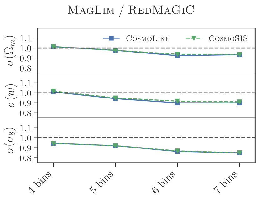
Figure 15: Standard deviations on $\Omega_{m}$, $w$ and $\sigma_{8}$ from different tomographic binnings of the MagLim sample normalized by estimates from the redMaGiC sample. The constraints have been obtained using two different codes for the covariances: CosmoLike and CosmoSIS.

Throughout this work we use the CosmoLike and CosmoSIS codes interchangeably to compute the Gaussian analytical covariances we use for our forecasts. Here we compare the constraints obtained using covariances estimated from the two codes. In Figure 15 we show the relative gain on $\Omega_{m}$, $w$ and $\sigma_{8}$ errors compared to redMaGiC for different tomographic binnings of the MagLim sample (see Sec. VI.1). We compare the estimates using a covariance from CosmoLike (solid blue) with those obtained using a covariance from CosmoSIS (dashed green), finding no difference in the constraints.

References

- Rozo et al. [2016] E. Rozo, E. S. Rykoff, A. Abate, C. Bonnett, M. Crocce, C. Davis, B. Hoyle, B. Leistedt, H. V. Peiris, R. H. Wechsler, et al., “redMaGiC: selecting luminous red galaxies from the DES Science Verification data,” MNRAS 461, 1431–1450 (2016), arXiv:1507.05460 [astro-ph.IM] .
- Frieman et al. [2008] J. A. Frieman, M. S. Turner, and D. Huterer, “Dark energy and the accelerating universe.” ARA&A 46, 385–432 (2008), arXiv:0803.0982 [astro-ph] .
- Spergel et al. [2003] D. N. Spergel, L. Verde, H. V. Peiris, E. Komatsu, M. R. Nolta, C. L. Bennett, M. Halpern, G. Hinshaw, N. Jarosik, A. Kogut, et al., “First-Year Wilkinson Microwave Anisotropy Probe (WMAP) Observations: Determination of Cosmological Parameters,” ApJS 148, 175–194 (2003), arXiv:astro-ph/0302209 [astro-ph] .
- Planck Collaboration et al. [2018] Planck Collaboration, N. Aghanim, et al., “Planck 2018 results. VI. Cosmological parameters,” arXiv e-prints , arXiv:1807.06209 (2018), arXiv:1807.06209 [astro-ph.CO] .
- Riess et al. [1998] Adam G. Riess, Alexei V. Filippenko, Peter Challis, Alejandro Clocchiatti, Alan Diercks, Peter M. Garnavich, Ron L. Gilliland, Craig J. Hogan, Saurabh Jha, Robert P. Kirshner, et al., “Observational Evidence from Supernovae for an Accelerating Universe and a Cosmological Constant,” AJ 116, 1009–1038 (1998), arXiv:astro-ph/9805201 [astro-ph] .
- Perlmutter et al. [1999] S. Perlmutter, G. Aldering, G. Goldhaber, R. A. Knop, P. Nugent, P. G. Castro, S. Deustua, S. Fabbro, A. Goobar, D. E. Groom, et al., “Measurements of and from 42 High-Redshift Supernovae,” ApJ 517, 565–586 (1999), arXiv:astro-ph/9812133 [astro-ph] .
- Tegmark et al. [2006] Max Tegmark, Daniel J. Eisenstein, Michael A. Strauss, David H. Weinberg, Michael R. Blanton, Joshua A. Frieman, Masataka Fukugita, James E. Gunn, Andrew J. S. Hamilton, Gillian R. Knapp, et al., “Cosmological constraints from the SDSS luminous red galaxies,” Phys. Rev. D 74, 123507 (2006), arXiv:astro-ph/0608632 [astro-ph] .
- Alam et al. [2017] Shadab Alam et al., “The clustering of galaxies in the completed SDSS-III Baryon Oscillation Spectroscopic Survey: cosmological analysis of the DR12 galaxy sample,” MNRAS 470, 2617–2652 (2017), arXiv:1607.03155 [astro-ph.CO] .
- DES Collaboration et al. [2019] DES Collaboration, T. M. C. Abbott, et al., “Cosmological Constraints from Multiple Probes in the Dark Energy Survey,” Phys. Rev. Lett. 122, 171301 (2019), arXiv:1811.02375 [astro-ph.CO] .
- Ivanov et al. [2020] Mikhail M. Ivanov, Marko Simonović, and Matias Zaldarriaga, “Cosmological parameters from the BOSS galaxy power spectrum,” J. Cosmology Astropart. Phys 2020, 042 (2020), arXiv:1909.05277 [astro-ph.CO] .
- d’Amico et al. [2020] Guido d’Amico, Jérôme Gleyzes, Nickolas Kokron, Katarina Markovic, Leonardo Senatore, Pierre Zhang, Florian Beutler, and Héctor Gil-Marín, “The cosmological analysis of the SDSS/BOSS data from the Effective Field Theory of Large-Scale Structure,” J. Cosmology Astropart. Phys 2020, 005 (2020), arXiv:1909.05271 [astro-ph.CO] .
- DES Collaboration et al. [2018a] DES Collaboration, T. M. C. Abbott, et al., “Dark Energy Survey year 1 results: Cosmological constraints from galaxy clustering and weak lensing,” Phys. Rev. D 98, 043526 (2018a), arXiv:1708.01530 [astro-ph.CO] .
- Joudaki et al. [2018] Shahab Joudaki, Chris Blake, Andrew Johnson, Alexandra Amon, Marika Asgari, Ami Choi, Thomas Erben, Karl Glazebrook, Joachim Harnois-Déraps, Catherine Heymans, et al., “KiDS-450 + 2dFLenS: Cosmological parameter constraints from weak gravitational lensing tomography and overlapping redshift-space galaxy clustering,” MNRAS 474, 4894–4924 (2018), arXiv:1707.06627 [astro-ph.CO] .
- van Uitert et al. [2018] Edo van Uitert, Benjamin Joachimi, Shahab Joudaki, Alexandra Amon, Catherine Heymans, Fabian Köhlinger, Marika Asgari, Chris Blake, Ami Choi, Thomas Erben, et al., “KiDS+GAMA: cosmology constraints from a joint analysis of cosmic shear, galaxy-galaxy lensing, and angular clustering,” MNRAS 476, 4662–4689 (2018), arXiv:1706.05004 [astro-ph.CO] .
- Hikage et al. [2019] Chiaki Hikage, Masamune Oguri, Takashi Hamana, Surhud More, Rachel Mandelbaum, Masahiro Takada, Fabian Köhlinger, Hironao Miyatake, Atsushi J. Nishizawa, Hiroaki Aihara, et al., “Cosmology from cosmic shear power spectra with Subaru Hyper Suprime-Cam first-year data,” PASJ 71, 43 (2019), arXiv:1809.09148 [astro-ph.CO] .
- Hamana et al. [2020] Takashi Hamana, Masato Shirasaki, Satoshi Miyazaki, Chiaki Hikage, Masamune Oguri, Surhud More, Robert Armstrong, Alexie Leauthaud, Rachel Mandelbaum, Hironao Miyatake, et al., “Cosmological constraints from cosmic shear two-point correlation functions with HSC survey first-year data,” PASJ 72, 16 (2020), arXiv:1906.06041 [astro-ph.CO] .
- Ivezić et al. [2019] Željko Ivezić, Steven M. Kahn, J. Anthony Tyson, Bob Abel, Emily Acosta, Robyn Allsman, David Alonso, Yusra AlSayyad, Scott F. Anderson, John Andrew, et al., “LSST: From Science Drivers to Reference Design and Anticipated Data Products,” ApJ 873, 111 (2019), arXiv:0805.2366 [astro-ph] .
- Laureijs et al. [2011] R. Laureijs, J. Amiaux, S. Arduini, J. L. Auguères, J. Brinchmann, R. Cole, M. Cropper, C. Dabin, L. Duvet, A. Ealet, et al., “Euclid Definition Study Report,” arXiv e-prints , f (2011), arXiv:1110.3193 [astro-ph.CO] .
- Spergel et al. [2015] D. Spergel, N. Gehrels, C. Baltay, D. Bennett, J. Breckinridge, M. Donahue, A. Dressler, B. S. Gaudi, T. Greene, O. Guyon, et al., “Wide-Field InfrarRed Survey Telescope-Astrophysics Focused Telescope Assets WFIRST-AFTA 2015 Report,” arXiv e-prints (2015), arXiv:1503.03757 [astro-ph.IM] .
- Eifler et al. [2020a] Tim Eifler, Melanie Simet, Elisabeth Krause, et al., “Cosmology with the Wide-Field Infrared Survey Telescope – Synergies with the Rubin Observatory Legacy Survey of Space and Time,” arXiv e-prints , arXiv:2004.04702 (2020a), arXiv:2004.04702 [astro-ph.CO] .
- Eifler et al. [2020b] Tim Eifler, Hironao Miyatake, Elisabeth Krause, et al., “Cosmology with the Wide-Field Infrared Survey Telescope – Multi-Probe Strategies,” arXiv e-prints , arXiv:2004.05271 (2020b), arXiv:2004.05271 [astro-ph.CO] .
- Bartelmann and Schneider [2001] M. Bartelmann and P. Schneider, “Weak gravitational lensing,” Phys. Rep. 340, 291–472 (2001), arXiv:astro-ph/9912508 [astro-ph] .
- Heymans et al. [2020] Catherine Heymans, Tilman Tröster, et al., “KiDS-1000 Cosmology: Multi-probe weak gravitational lensing and spectroscopic galaxy clustering constraints,” arXiv e-prints , arXiv:2007.15632 (2020), arXiv:2007.15632 [astro-ph.CO] .
- Eisenstein et al. [2001] Daniel J. Eisenstein, James Annis, James E. Gunn, Alexander S. Szalay, Andrew J. Connolly, R. C. Nichol, Neta A. Bahcall, Mariangela Bernardi, Scott Burles, Francisco J. Castander, et al., “Spectroscopic Target Selection for the Sloan Digital Sky Survey: The Luminous Red Galaxy Sample,” AJ 122, 2267–2280 (2001), arXiv:astro-ph/0108153 [astro-ph] .
- Padmanabhan et al. [2007] Nikhil Padmanabhan, David J. Schlegel, Uroš Seljak, Alexey Makarov, Neta A. Bahcall, Michael R. Blanton, Jonathan Brinkmann, Daniel J. Eisenstein, Douglas P. Finkbeiner, James E. Gunn, et al., “The clustering of luminous red galaxies in the Sloan Digital Sky Survey imaging data,” MNRAS 378, 852–872 (2007), arXiv:astro-ph/0605302 [astro-ph] .
- Vakili and Hoekstra [2020] Mohammadjavad Vakili and Henk andothers Hoekstra, “Clustering of red-sequence galaxies in the fourth data release ofthe Kilo-Degree Survey,” arXiv e-prints , arXiv:2008.13154 (2020), arXiv:2008.13154 [astro-ph.CO] .
- Crocce et al. [2019] M. Crocce, A. J. Ross, I. Sevilla-Noarbe, E. Gaztanaga, J. Elvin-Poole, S. Avila, A. Alarcon, K. C. Chan, N. Banik, J. Carretero, et al., “Dark Energy Survey year 1 results: galaxy sample for BAO measurement,” MNRAS 482, 2807–2822 (2019), arXiv:1712.06211 [astro-ph.CO] .
- Sridhar et al. [2020] Srivatsan Sridhar, Yong-Seon Song, Ashley J. Ross, Rongpu Zhou, Jeffrey A. Newman, Chia-Hsun Chuang, Francisco Prada, Robert Blum, Enrique Gaztañaga, and Martin Landriau, “The clustering of LRGs in the DECaLS DR8 footprint: distance constraints from baryon acoustic oscillations using photometric redshifts,” arXiv e-prints , arXiv:2005.13126 (2020), arXiv:2005.13126 [astro-ph.CO] .
- Crocce et al. [2016] M. Crocce, J. Carretero, A. H. Bauer, A. J. Ross, I. Sevilla-Noarbe, T. Giannantonio, F. Sobreira, J. Sanchez, E. Gaztanaga, M. C. Kind, et al., “Galaxy clustering, photometric redshifts and diagnosis of systematics in the DES Science Verification data,” MNRAS 455, 4301–4324 (2016), arXiv:1507.05360 .
- Coupon et al. [2012] J. Coupon, M. Kilbinger, H. J. McCracken, O. Ilbert, S. Arnouts, Y. Mellier, U. Abbas, S. de la Torre, Y. Goranova, P. Hudelot, J. P. Kneib, and O. Le Fèvre, “Galaxy clustering in the CFHTLS-Wide: the changing relationship between galaxies and haloes since z ~1.2,” A&A 542, A5 (2012), arXiv:1107.0616 [astro-ph.CO] .
- Nicola et al. [2020] Andrina Nicola, David Alonso, Javier Sánchez, Anže Slosar, et al., “Tomographic galaxy clustering with the Subaru Hyper Suprime-Cam first year public data release,” J. Cosmology Astropart. Phys 2020, 044 (2020), arXiv:1912.08209 [astro-ph.CO] .
- Porredon et al. [in prep.] A. Porredon et al., “Dark Energy Survey Year 3 Results: Cosmological Constraints from Galaxy Clustering and Galaxy-Galaxy Lensing using an Optimized Lens Sample,” to be submitted to PRD (in prep.).
- Flaugher et al. [2015] B. Flaugher, H. T. Diehl, K. Honscheid, T. M. C. Abbott, O. Alvarez, R. Angstadt, J. T. Annis, M. Antonik, O. Ballester, L. Beaufore, et al., “The Dark Energy Camera,” AJ 150, 150 (2015), arXiv:1504.02900 [astro-ph.IM] .
- Sevilla-Noarbe et al. [2020] I. Sevilla-Noarbe, K. Bechtol, M. Carrasco Kind, et al., “Dark Energy Survey Year 3 Results: Photometric Data Set for Cosmology,” arXiv e-prints , arXiv:2011.03407 (2020), arXiv:2011.03407 [astro-ph.CO] .
- DES Collaboration et al. [2018b] DES Collaboration, T. M. C. Abbott, et al., “The dark energy survey: Data release 1,” The Astrophysical Journal Supplement Series 239, 18 (2018b).
- Morganson et al. [2018] E. Morganson, R. A. Gruendl, F. Menanteau, M. Carrasco Kind, Y.-C. Chen, G. Daues, A. Drlica-Wagner, D. N. Friedel, M. Gower, M. W. G. Johnson, et al., “The Dark Energy Survey Image Processing Pipeline,” PASP 130, 074501 (2018), arXiv:1801.03177 [astro-ph.IM] .
- Burke et al. [2018] D. L. Burke, E. S. Rykoff, S. Allam, J. Annis, K. Bechtol, G. M. Bernstein, A. Drlica-Wagner, D. A. Finley, R. A. Gruendl, D. J. James, et al., “Forward Global Photometric Calibration of the Dark Energy Survey,” AJ 155, 41 (2018), arXiv:1706.01542 [astro-ph.IM] .
- Bertin and Arnouts [1996] E. Bertin and S. Arnouts, “SExtractor: Software for source extraction.” A&AS 117, 393–404 (1996).
- Troxel et al. [2018] M. A. Troxel, N. MacCrann, J. Zuntz, T. F. Eifler, E. Krause, S. Dodelson, D. Gruen, J. Blazek, O. Friedrich, S. Samuroff, et al., “Dark Energy Survey Year 1 results: Cosmological constraints from cosmic shear,” Phys. Rev. D 98, 043528 (2018), arXiv:1708.01538 [astro-ph.CO] .
- Drlica-Wagner et al. [2018] A. Drlica-Wagner, I. Sevilla-Noarbe, E. S. Rykoff, R. A. Gruendl, B. Yanny, D. L. Tucker, B. Hoyle, A. Carnero Rosell, G. M. Bernstein, K. Bechtol, et al., “Dark Energy Survey Year 1 Results: The Photometric Data Set for Cosmology,” ApJS 235 (2018), 10.3847/1538-4365/aab4f5.
- Benítez [2000] N. Benítez, “Bayesian Photometric Redshift Estimation,” ApJ 536, 571–583 (2000), astro-ph/9811189 .
- Sadeh et al. [2016] I. Sadeh, F. B. Abdalla, and O. Lahav, “ANNz2: Photometric Redshift and Probability Distribution Function Estimation using Machine Learning,” PASP 128, 104502 (2016), arXiv:1507.00490 .
- De Vicente et al. [2016] J. De Vicente, E. Sánchez, and I. Sevilla-Noarbe, “DNF - Galaxy photometric redshift by Directional Neighbourhood Fitting,” MNRAS 459, 3078–3088 (2016), arXiv:1511.07623 [astro-ph.CO] .
- Gschwend et al. [2018] J. Gschwend, A. C. Rossel, R. L. C. Ogando, A. F. Neto, M. A. G. Maia, L. N. da Costa, M. Lima, P. Pellegrini, R. Campisano, C. Singulani, et al., “DES science portal: Computing photometric redshifts,” Astronomy and Computing 25, 58–80 (2018), arXiv:1708.05643 [astro-ph.GA] .
- SDSS Collaboration et al. [2018] SDSS Collaboration, Bela Abolfathi, et al., “The Fourteenth Data Release of the Sloan Digital Sky Survey: First Spectroscopic Data from the Extended Baryon Oscillation Spectroscopic Survey and from the Second Phase of the Apache Point Observatory Galactic Evolution Experiment,” ApJS 235, 42 (2018), arXiv:1707.09322 [astro-ph.GA] .
- Childress et al. [2017] M. J. Childress, C. Lidman, T. M. Davis, B. E. Tucker, J. Asorey, F. Yuan, T. M. C. Abbott, F. B. Abdalla, S. Allam, J. Annis, et al., “OzDES multifibre spectroscopy for the Dark Energy Survey: 3-yr results and first data release,” MNRAS 472, 273–288 (2017), arXiv:1708.04526 [astro-ph.CO] .
- Garilli et al. [2014] B. Garilli, L. Guzzo, M. Scodeggio, M. Bolzonella, U. Abbas, C. Adami, S. Arnouts, J. Bel, D. Bottini, E. Branchini, et al., “The VIMOS Public Extragalactic Survey (VIPERS). First Data Release of 57 204 spectroscopic measurements,” A&A 562, A23 (2014), arXiv:1310.1008 .
- Tanoglidis et al. [2020] Dimitrios Tanoglidis, Chihway Chang, and Joshua Frieman, “Optimizing galaxy samples for clustering measurements in photometric surveys,” MNRAS 491, 3535–3552 (2020), arXiv:1908.07150 [astro-ph.CO] .
- Rodríguez-Monroy et al. [in prep.] M. Rodríguez-Monroy et al., “Dark Energy Survey Year 3 Results: Galaxy clustering and systematics treatment for lens galaxy samples,” to be submitted to MNRAS (in prep.).
- Rykoff et al. [2014] E. S. Rykoff, E. Rozo, M. T. Busha, C. E. Cunha, A. Finoguenov, A. Evrard, J. Hao, B. P. Koester, A. Leauthaud, B. Nord, M. Pierre, R. Reddick, T. Sadibekova, E. S. Sheldon, and R. H. Wechsler, “redMaPPer. I. Algorithm and SDSS DR8 Catalog,” ApJ 785, 104 (2014), arXiv:1303.3562 [astro-ph.CO] .
- Rykoff et al. [2016] E. S. Rykoff, E. Rozo, D. Hollowood, A. Bermeo-Hernand ez, T. Jeltema, J. Mayers, A. K. Romer, P. Rooney, A. Saro, C. Vergara Cervantes, et al., “The RedMaPPer Galaxy Cluster Catalog From DES Science Verification Data,” ApJS 224, 1 (2016), arXiv:1601.00621 [astro-ph.CO] .
- Bruzual and Charlot [2003] G. Bruzual and S. Charlot, “Stellar population synthesis at the resolution of 2003,” MNRAS 344, 1000–1028 (2003), arXiv:astro-ph/0309134 [astro-ph] .
- Elvin-Poole et al. [2018] J. Elvin-Poole, M. Crocce, A. J. Ross, T. Giannantonio, E. Rozo, E. S. Rykoff, S. Avila, N. Banik, J. Blazek, S. L. Bridle, et al., “Dark Energy Survey year 1 results: Galaxy clustering for combined probes,” Phys. Rev. D 98, 042006 (2018), arXiv:1708.01536 [astro-ph.CO] .
- Hoyle et al. [2018] B. Hoyle, D. Gruen, G. M. Bernstein, M. M. Rau, J. De Vicente, W. G. Hartley, E. Gaztanaga, J. DeRose, M. A. Troxel, C. Davis, et al., “Dark Energy Survey Year 1 Results: redshift distributions of the weak-lensing source galaxies,” MNRAS 478, 592–610 (2018), arXiv:1708.01532 [astro-ph.CO] .
- Gatti et al. [2018] M. Gatti, P. Vielzeuf, et al., “Dark Energy Survey Year 1 results: cross-correlation redshifts - methods and systematics characterization,” MNRAS 477, 1664–1682 (2018), arXiv:1709.00992 [astro-ph.CO] .
- Lima et al. [2008] Marcos Lima, Carlos E. Cunha, Hiroaki Oyaizu, Joshua Frieman, Huan Lin, and Erin S. Sheldon, “Estimating the redshift distribution of photometric galaxy samples,” MNRAS 390, 118–130 (2008), arXiv:0801.3822 [astro-ph] .
- Cawthon et al. [2020] R. Cawthon, J. Elvin-Poole, A. Porredon, M. Crocce, G. Giannini, M. Gatti, A. J. Ross, E. S. Rykoff, A. Carnero Rosell, J. DeRose, S. Lee, M. Rodriguez-Monroy, et al., “Dark Energy Survey Year 3 Results: Calibration of Lens Sample Redshift Distributions using Clustering Redshifts with BOSS/eBOSS,” arXiv e-prints , arXiv:2012.12826 (2020), arXiv:2012.12826 [astro-ph.CO] .
- Tegmark et al. [1997] Max Tegmark, Andy N. Taylor, and Alan F. Heavens, “Karhunen-Loève Eigenvalue Problems in Cosmology: How Should We Tackle Large Data Sets?” ApJ 480, 22–35 (1997), arXiv:astro-ph/9603021 [astro-ph] .
- Tegmark [1997] Max Tegmark, “Measuring Cosmological Parameters with Galaxy Surveys,” Phys. Rev. Lett. 79, 3806–3809 (1997), arXiv:astro-ph/9706198 [astro-ph] .
- Wolz et al. [2012] Laura Wolz, Martin Kilbinger, Jochen Weller, and Tommaso Giannantonio, “On the validity of cosmological Fisher matrix forecasts,” J. Cosmology Astropart. Phys 2012, 009 (2012), arXiv:1205.3984 [astro-ph.CO] .
- Camera et al. [2017] Stefano Camera, Ian Harrison, Anna Bonaldi, and Michael L. Brown, “SKA weak lensing - III. Added value of multiwavelength synergies for the mitigation of systematics,” MNRAS 464, 4747–4760 (2017), arXiv:1606.03451 [astro-ph.CO] .
- Euclid Collaboration et al. [2019] Euclid Collaboration, A. Blanchard, et al., “Euclid preparation: VII. Forecast validation for Euclid cosmological probes,” arXiv e-prints , arXiv:1910.09273 (2019), arXiv:1910.09273 [astro-ph.CO] .
- Yahia-Cherif et al. [2020] S. Yahia-Cherif, A. Blanchard, S. Camera, S. Ilić, K. Markovič, A. Pourtsidou, Z. Sakr, D. Sapone, and I. Tutusaus, “Validating the Fisher approach for stage IV spectroscopic surveys,” arXiv e-prints , arXiv:2007.01812 (2020), arXiv:2007.01812 [astro-ph.CO] .
- Zuntz et al. [2015] J. Zuntz, M. Paterno, E. Jennings, D. Rudd, A. Manzotti, S. Dodelson, S. Bridle, S. Sehrish, and J. Kowalkowski, “CosmoSIS: Modular cosmological parameter estimation,” Astronomy and Computing 12, 45–59 (2015), arXiv:1409.3409 .
- Feroz et al. [2009] F. Feroz, M. P. Hobson, and M. Bridges, “MULTINEST: an efficient and robust Bayesian inference tool for cosmology and particle physics,” MNRAS 398, 1601–1614 (2009), arXiv:0809.3437 [astro-ph] .
- LoVerde and Afshordi [2008] Marilena LoVerde and Niayesh Afshordi, “Extended Limber approximation,” Physical Review D 78, 123506 (2008), arXiv:0809.5112 [astro-ph] .
- Hirata and Seljak [2004] Christopher M. Hirata and Uroš Seljak, “Intrinsic alignment-lensing interference as a contaminant of cosmic shear,” Phys. Rev. D 70, 063526 (2004), arXiv:astro-ph/0406275 [astro-ph] .
- Bridle and King [2007] Sarah Bridle and Lindsay King, “Dark energy constraints from cosmic shear power spectra: impact of intrinsic alignments on photometric redshift requirements,” New Journal of Physics 9, 444 (2007), arXiv:0705.0166 [astro-ph] .
- Elvin-Poole et al. [in prep.] J. Elvin-Poole et al., “Dark Energy Survey Year 3 Results: Measurement, modelling and cosmological impact of magnification in galaxy clustering and galaxy-galaxy lensing,” to be submitted to MNRAS (in prep.).
- Lewis et al. [2000] Antony Lewis, Anthony Challinor, and Anthony Lasenby, “Efficient Computation of Cosmic Microwave Background Anisotropies in Closed Friedmann‐Robertson‐Walker Models,” The Astrophysical Journal 538, 473–476 (2000), arXiv:9911177 [astro-ph] .
- Howlett et al. [2012] Cullan Howlett, Antony Lewis, Alex Hall, and Anthony Challinor, “CMB power spectrum parameter degeneracies in the era of precision cosmology,” Journal of Cosmology and Astroparticle Physics 2012, 027–027 (2012), arXiv:1201.3654 .
- Smith et al. [2003] R. E. Smith, J. A. Peacock, A. Jenkins, S. D. M. White, C. S. Frenk, F. R. Pearce, P. A. Thomas, G. Efstathiou, and H. M. P. Couchman, “Stable clustering, the halo model and non-linear cosmological power spectra,” MNRAS 341, 1311–1332 (2003), astro-ph/0207664 .
- Takahashi et al. [2012] R. Takahashi, M. Sato, T. Nishimichi, A. Taruya, and M. Oguri, “Revising the Halofit Model for the Nonlinear Matter Power Spectrum,” ApJ 761, 152 (2012), arXiv:1208.2701 .
- Bird et al. [2012] Simeon Bird, Matteo Viel, and Martin G. Haehnelt, “Massive neutrinos and the non-linear matter power spectrum,” MNRAS 420, 2551–2561 (2012), arXiv:1109.4416 [astro-ph.CO] .
- Krause et al. [2017] E. Krause, T. F. Eifler, J. Zuntz, O. Friedrich, M. A. Troxel, S. Dodelson, J. Blazek, L. F. Secco, N. MacCrann, E. Baxter, et al., “Dark Energy Survey Year 1 Results: Multi-Probe Methodology and Simulated Likelihood Analyses,” arXiv e-prints , arXiv:1706.09359 (2017), arXiv:1706.09359 [astro-ph.CO] .
- Fang et al. [2020a] Xiao Fang, Tim Eifler, and Elisabeth Krause, “2D-FFTLog: efficient computation of real-space covariance matrices for galaxy clustering and weak lensing,” MNRAS 497, 2699–2714 (2020a), arXiv:2004.04833 [astro-ph.CO] .
- Cooray and Sheth [2002] Asantha Cooray and Ravi Sheth, “Halo models of large scale structure,” Phys. Rep. 372, 1–129 (2002), arXiv:astro-ph/0206508 [astro-ph] .
- Takada and Jain [2009] Masahiro Takada and Bhuvnesh Jain, “The impact of non-Gaussian errors on weak lensing surveys,” MNRAS 395, 2065–2086 (2009), arXiv:0810.4170 [astro-ph] .
- Takada and Hu [2013] Masahiro Takada and Wayne Hu, “Power spectrum super-sample covariance,” Phys. Rev. D 87, 123504 (2013), arXiv:1302.6994 [astro-ph.CO] .
- Hu and Jain [2004] Wayne Hu and Bhuvnesh Jain, “Joint galaxy-lensing observables and the dark energy,” Phys. Rev. D 70, 043009 (2004), arXiv:astro-ph/0312395 [astro-ph] .
- Crocce et al. [2011] Martín Crocce, Anna Cabré, and Enrique Gaztañaga, “Modelling the angular correlation function and its full covariance in photometric galaxy surveys,” MNRAS 414, 329–349 (2011), arXiv:1004.4640 [astro-ph.CO] .
- Joachimi et al. [2008] B. Joachimi, P. Schneider, and T. Eifler, “Analysis of two-point statistics of cosmic shear. III. Covariances of shear measures made easy,” A&A 477, 43–54 (2008), arXiv:0708.0387 [astro-ph] .
- Krause and Eifler [2017] Elisabeth Krause and Tim Eifler, “cosmolike - cosmological likelihood analyses for photometric galaxy surveys,” MNRAS 470, 2100–2112 (2017), arXiv:1601.05779 [astro-ph.CO] .
- Particle Data Group et al. [2016] Particle Data Group, C. Patrignani, et al., “Review of Particle Physics,” Chinese Physics C 40, 100001 (2016).
- Muir et al. [2020] J. Muir, G. M. Bernstein, D. Huterer, F. Elsner, E. Krause, Roodman, et al., “Blinding multiprobe cosmological experiments,” MNRAS 494, 4454–4470 (2020), arXiv:1911.05929 [astro-ph.CO] .
- Cawthon et al. [2018] R. Cawthon, C. Davis, M. Gatti, P. Vielzeuf, et al., “Dark Energy Survey Year 1 Results: calibration of redMaGiC redshift distributions in DES and SDSS from cross-correlations,” MNRAS 481, 2427–2443 (2018), arXiv:1712.07298 [astro-ph.CO] .
- Cui et al. [2014] Weiguang Cui, Stefano Borgani, and Giuseppe Murante, “The effect of active galactic nuclei feedback on the halo mass function,” MNRAS 441, 1769–1782 (2014), arXiv:1402.1493 [astro-ph.CO] .
- Velliscig et al. [2014] Marco Velliscig, Marcel P. van Daalen, Joop Schaye, Ian G. McCarthy, Marcello Cacciato, Amandine M. C. Le Brun, and Claudio Dalla Vecchia, “The impact of galaxy formation on the total mass, mass profile and abundance of haloes,” MNRAS 442, 2641–2658 (2014), arXiv:1402.4461 [astro-ph.CO] .
- Mummery et al. [2017] Benjamin O. Mummery, Ian G. McCarthy, Simeon Bird, and Joop Schaye, “The separate and combined effects of baryon physics and neutrino free streaming on large-scale structure,” MNRAS 471, 227–242 (2017), arXiv:1702.02064 [astro-ph.CO] .
- van Daalen et al. [2011] Marcel P. van Daalen, Joop Schaye, C. M. Booth, and Claudio Dalla Vecchia, “The effects of galaxy formation on the matter power spectrum: a challenge for precision cosmology,” MNRAS 415, 3649–3665 (2011), arXiv:1104.1174 [astro-ph.CO] .
- DES and SPT Collaborations et al. [2019] DES and SPT Collaborations, T. M. C. Abbott, et al., “Dark Energy Survey year 1 results: Joint analysis of galaxy clustering, galaxy lensing, and CMB lensing two-point functions,” Phys. Rev. D 100, 023541 (2019), arXiv:1810.02322 [astro-ph.CO] .
- Asorey et al. [2012] Jacobo Asorey, Martin Crocce, Enrique Gaztañaga, and Antony Lewis, “Recovering 3D clustering information with angular correlations,” MNRAS 427, 1891–1902 (2012), arXiv:1207.6487 [astro-ph.CO] .
- Fang et al. [2020b] Xiao Fang, Elisabeth Krause, Tim Eifler, and Niall MacCrann, “Beyond Limber: efficient computation of angular power spectra for galaxy clustering and weak lensing,” J. Cosmology Astropart. Phys 2020, 010 (2020b), arXiv:1911.11947 [astro-ph.CO] .
- MacCrann et al. [2020] Niall MacCrann, Jonathan Blazek, Bhuvnesh Jain, and Elisabeth Krause, “Controlling and leveraging small-scale information in tomographic galaxy-galaxy lensing,” MNRAS 491, 5498–5509 (2020), arXiv:1903.07101 [astro-ph.CO] .
- Fang et al. [2020c] Xiao Fang, Tim Eifler, and Elisabeth Krause, “2D-FFTLog: Efficient computation of real space covariance matrices for galaxy clustering and weak lensing,” arXiv e-prints , arXiv:2004.04833 (2020c), arXiv:2004.04833 [astro-ph.CO] .
- Center [1987] Ohio Supercomputer Center, “Ohio supercomputer center,” (1987).
- Raveri et al. [2016a] Marco Raveri, Matteo Martinelli, Gongbo Zhao, and Yuting Wang, “CosmicFish Implementation Notes V1.0,” arXiv e-prints , arXiv:1606.06268 (2016a), arXiv:1606.06268 [astro-ph.CO] .
- Raveri et al. [2016b] Marco Raveri, Matteo Martinelli, Gongbo Zhao, and Yuting Wang, “Information Gain in Cosmology: From the Discovery of Expansion to Future Surveys,” arXiv e-prints , arXiv:1606.06273 (2016b), arXiv:1606.06273 [astro-ph.CO] .
- Hinton [2016] S. R. Hinton, “ChainConsumer,” The Journal of Open Source Software 1, 00045 (2016).