Outbreak diversity in epidemic waves propagating through distinct geographical scales

Abstract

A central feature of an emerging infectious disease in a pandemic scenario is the spread through geographical scales and the impacts on different locations according to the adopted mitigation protocols. We investigated a stochastic epidemic model with the metapopulation approach in which patches represent municipalities. Contagion follows a stochastic compartmental model for municipalities; the latter, in turn, interact with each other through recurrent mobility. As a case of study, we consider the epidemic of COVID-19 in Brazil performing data-driven simulations. Properties of the simulated epidemic curves have very broad distributions across different geographical locations and scales, from states, passing through intermediate and immediate regions down to municipality levels. Correlations between delay of the epidemic outbreak and distance from the respective capital cities were predicted to be strong in several states and weak in others, signaling influences of multiple epidemic foci propagating towards the inland cities. Responses of different regions to a same mitigation protocol can vary enormously implying that the policies of combating the epidemics must be engineered according to the region’ specificity but integrated with the overall situation. Real series of reported cases confirm the qualitative scenarios predicted in simulations. Even though we restricted our study to Brazil, the prospects and model can be extended to other geographical organizations with heterogeneous demographic distributions.

I Introduction

Theoretical and computational toolboxes used and developed by physicists over decades and, in particular, those of equilibrium and nonequilibrium statistical physics have found an inexhaustible source of applications in complexity Bak et al. (1988); Barabási (2005); Goldenfeld and Kadanoff (1999); Nowak and May (1992) attaining an apex with the raising of network science at late 1990s Barabási and Pósfai (2016). Epidemic models, which are intimately related with nonequilibrium phase transitions Henkel et al. (2008), running on the top of networks soon became one of the most imminent fields of interdisciplinary physics Pastor-Satorras and Vespignani (2001); Newman (2002); Pastor-Satorras et al. (2015) with many applications on real epidemic scenarios lead by physicists Colizza et al. (2006); Balcan et al. (2009); Wang et al. (2009). The pandemic of coronavirus disease (COVID-19) has been marked by a wide discussion heavily grounded on data-driven epidemic modeling, again with outstanding contributions lead by physicists Chinazzi et al. (2020); Kraemer et al. (2020); Gilbert et al. (2020); Arenas et al. (2020a).

Since COVID-19 outbreak was reported in Wuhan, Hubei province, China, at the end of December 2019, the scientific community has turned its attention to understanding and combating this novel threat Li et al. (2020a); Wu et al. (2020); Chinazzi et al. (2020); Li et al. (2020b); Kraemer et al. (2020). A characteristic of this infectious disease, caused by the pathogen coronavirus SARS-CoV-2, is the high transmission rate of individuals without significant symptoms Li et al. (2020b); Read et al. (2020) who traveled unrestrictedly and spread COVID-19 through all continents except Antarctica. Efforts to track the transmission from Wuhan to the rest of mainland China and world relied on mathematical modeling Chinazzi et al. (2020); Kraemer et al. (2020); Pullano et al. (2020); Wu et al. (2020); Aleta et al. (2020), which were soon extended to other countries Danon et al. (2020); Arenas et al. (2020b); Aleta and Moreno (2020), using the metapopulation approach Colizza et al. (2007a); Danon et al. (2009); Gómez-Gardeñes et al. (2018). In this modeling, the population is grouped in patches representing geographic regions and the epidemic contagion obeys standard compartmental models Diekmann and Heesterbeek (2000) within the patches, while mobility among them promotes the epidemic to spread through the whole population. Metapopulation approaches, which were initially conceived in ecology contexts Hanski (1989), have been used for many epidemic processes Colizza and Vespignani (2007); Colizza et al. (2007a); Watts et al. (2005); Lloyd and Jansen (2004); Danon et al. (2009); Gómez-Gardeñes et al. (2018); Meloni et al. (2011) and allow a geographical resolution absent in standard compartmental models Diekmann and Heesterbeek (2000). One remarkable feature of the metapopulation approach is its capability to integrate the epidemic modeling in different regions into a single framework, in which correlation between epidemic waves in different regions can be investigated.

We are interested on the geographical variability and impacts of an emerging and highly contagious infections disease such as the COVID-19 in continental scales and we chose the recent pandemics in Brazil as a case of study. Brazil is a country of continental territory with an area of $8.5\times 10^{6}$ km² demographically, economically, and developmentally very heterogeneous. It is a federation divided into 26 states and one Federal District, its capital city. States are divided into municipalities; each state has its own capital city. The total number of municipalities is 5570 and, according to estimates of 2019, the country population is approximately 210 million Instituto Brasileiro de Geografia e Estatística (2019) (IBGE). Striking characteristics of the Brazilian demography are the broad distributions of the rural and urban population fractions and urban population densities of municipalities, which are important traits in epidemic modeling Hu et al. (2013); Rocklöv and Sjödin (2020). Therefore, investigation of a pandemic and its consequences have necessarily to integrate the particularities of each region, which can be reckoned with the metapopulation approach.

In this work, we investigate a metapopulation model and applied it to the COVID-19 epidemic spread in the Brazilian municipalities. At the time of submission, early June 2020, the benchmark of 800 000 cases and 40 000 deaths was surpassed in Brazil, which became in this date the country with highest epidemic incidence and possibly a new worldwide epicenter of COVID-19 Cota (2020). At time of resubmission, mid October 2020, the number of cases had surpassed 5.5 millions with more than 150 000 deaths. The model is supplied by demographic and mobility data mined from public sources, which are used in the stochastic simulations. We quantify how diversified the epidemic can be across the country rather than try to accurately foresee outbreaks in specific locations. We determine the level of dispersion in the curves of the epidemic prevalence in different places within a hypothetical scenario of uniform mitigation measures. We take the situation of 31 March 2020 as the initial condition, with foci in 410 municipalities, allowing to track the epidemics in all municipalities in a single integrated simulation. We predicted that the prevalence curves can vary enormously over geographical scales ranging from states down to municipalities. We also predicted that some states are characterized by outbreaks starting mainly in their capital cities, followed by epidemic waves propagating toward the countryside, while in other states there are multiple epidemic foci. Our results explain why policies of combating a countrywide pandemic should be simultaneously decentralized, in the sense that each locality has to consider its specificities, and integrated, since the fate of one region depends on the attitudes adopted by others. These qualitative behaviors have been confirmed a posteriori.

The remaining of the paper is organized as follows. The model is described in Sec. II while its computer implementation and parameters are in Appendixes A and B, respectively. Model calibration using nowcasting is presented in Sec. III while the detailed results are in Sec. IV. Some discussions and remarks are presented in Sec. V. In Sec. VI, we present a brief afterwords commenting the achievements of the model in forecasting the qualitative countrywide behavior of the pandemics in Brazil five months after the predictions were made Costa et al. (2020).

II The model

II.1 Metapopulation

We consider a stochastic metapopulation model for the countrywide spread of the epidemic, in which a key ingredient is recurrent mobility Gómez-Gardeñes et al. (2018) whereby individuals travel to other patches but return to their residence recurrently. The population is divided into patches which represent the places of residence as schematically shown in Fig. 1a). Similar models have been used for modeling of COVID-19 in Spain Arenas et al. (2020b, a); Aleta and Moreno (2020). In particular, our model is inspired on a recent work Arenas et al. (2020b) to investigate the COVID-19. We use a different, continuous-time approach where geographical, demographical, and testing capacity specificities are included. As in general metapopulation models, a patch can represent a municipality, a neighborhood or any other demographic distribution of interest. Each patch is labeled by $i=1,2,\ldots,\Omega$, where $\Omega$ is the number of patches, and has a resident population fixed in time given by $N_{i}$. The inter-patch mobility rate is given by $W_{ij}$ defined as the number of individuals that travel from $i$ to $j$ and return to $i$ after a typical time $T_{\text{r}}$. A patch $j$ for which $W_{ij}>0$ is a neighbor of $i$. Different forms of mobility, with their corresponding characteristic times, can be implemented. For the sake of simplicity, recurrent flux of individuals per day ($T_{\text{r}}=1$ d) is used in the present work. Mobility within patches is not explicitly considered. Instead, we assume the well-mixed population hypothesis Diekmann and Heesterbeek (2000) where an individual has equal chance to be in contact with any other in the same patch.

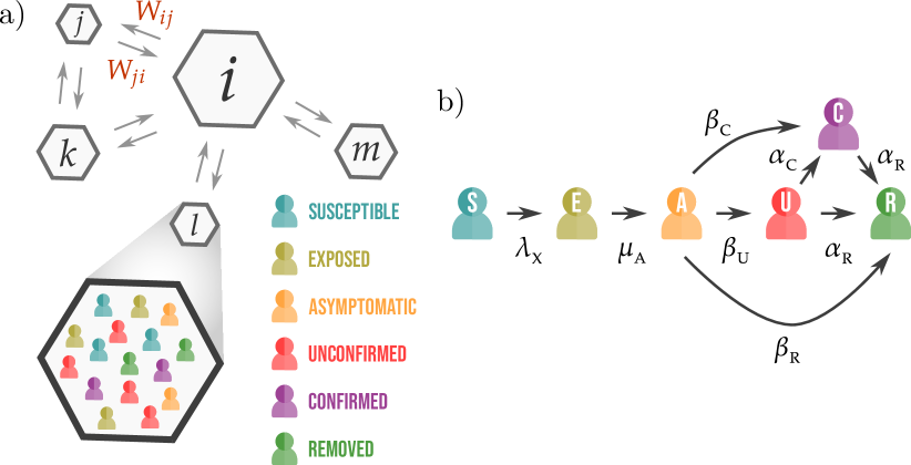
Figure 1: Schematic representation of a) metapopulation structure and b) epidemic transitions with their respective rates. Patches $i$ and $j$ of different population sizes (represented by the areas) can interchange individuals with rates $W_{ij}$ and $W_{ji}$. The epidemic events occur within patches under the hypothesis of well-mixed populations as illustrated in the zoom of patch $l$. Six compartments are used: susceptible (S), exposed (E), asymptomatic or presymptomatic (A), unconfirmed (U), confirmed (C), and removed (R). The infection rate per contact $\lambda_{\text{X}}$ can be of three forms, depending on the infectious contacts: S and A ($\lambda_{\text{A}}$), S and U ($\lambda_{\text{U}}$), and S and C ($\lambda_{\text{C}}$).

II.2 Demography and contacts

The average number of contacts per individual of patch $i$ per unit of time is $k_{i}$. Variations in the social distancing can be implemented by altering $k_{i}$. Contacts are related to local mobility and are strongly correlated with the population density $\xi_{i}$. Monotonic increase has been proposed Hu et al. (2013). We follow Ref. Arenas et al. (2020b) and use a contact number modulated by $k_{i}\propto f(\xi_{i})$ with $f(\xi)=2-\exp(-a\xi)$. To take into account the sparse demographic distribution of Brazil, we used the urban population density of each municipality to compute $\xi_{i}$. Interactions between urban and rural populations are also explicitly considered through a symmetric $2\times 2$ contact matrix $\mathcal{C}_{\text{uu}}$, $\mathcal{C}_{\text{rr}}$, and $\mathcal{C}_{\text{ur}}=\mathcal{C}_{\text{ru}}$, $0\leq\mathcal{C}_{\text{xy}}\leq 1$, determining the contacts between urban (u) and rural (r) populations whose fractions are represented by $\omega_{i}$ and $1-\omega_{i}$, respectively. The number of contacts in patch $i$ is also modulated by

$$k_{i}\propto g_{i}=\mathcal{C}_{\text{uu}}\omega_{i}^{2}+2\omega_{i}(1-\omega_{i})\mathcal{C}_{\text{ur}}+(1-\omega_{i})^{2}\mathcal{C}_{\text{rr}},$$ (1)

where the terms represent urban-urban, urban-rural, and rural-rural interactions from left to right. The contacts are parameterized by their average number per individual $\langle{k}\rangle$, such that $k_{i}=zg_{i}f(\xi_{i})\langle{k}\rangle$, where $z$ is a normalization factor, required by the relation $\sum_{i}k_{i}N_{i}=N_{\text{tot}}\langle{k}\rangle$ and given by

$$z=\frac{N_{\text{tot}}}{\sum_{i=1}^{\Omega}f(\xi_{i})g_{i}N_{i}},$$ (2)

where $N_{\text{tot}}=\sum_{i}N_{i}$ is the total population.

II.3 Epidemic model

The epidemic dynamics within the patches considers three noncontagious compartments which are: susceptible (S), that can be infected; removed (R), that represents immunized or deceased individuals; and exposed (E) that carries the virus but does not transmit it. Compartments of contagious individuals are: asymptomatic (A), that have not presented symptoms; unconfirmed (U), which are symptomatic but not yet identified by tests; and confirmed (C), that have tested positive for COVID-19. The compartment A is actually a simplification of the real situation. At least two relevant types of asymptomatic persons do exist: presymptomatic, that will develop symptoms at the end of the incubation period, and the truly asymptomatic, that becomes recovered without any significant symptoms. There exist large uncertainties with respect to the fraction of individuals who are truly asymptomatic Byambasuren et al. (2020); Casey et al. (2020). According to the parameters used in this work (see Appendix B), we have approximated 30% of truly asymptomatic in compartment A which lies within the interval reported elsewhere Byambasuren et al. (2020). Due to the uncertainty of the available data, we also assume a same contagion rate for both types of asymptomatic individuals which are hereafter treated as a single compartment. The epidemic transitions obey a SEAUCR model, in which susceptible individuals become exposed by contact with contagious persons (A, U, or C) with rates $\lambda_{\text{A}}$, $\lambda_{\text{U}}$, and $\lambda_{\text{C}}$, respectively. Exposed individuals spontaneously become asymptomatic with rate $\mu_{\text{A}}$, while the latter transitions to unconfirmed (presymptomatic), confirmed, or removed (truly asymptomatic) states happen with rates $\beta_{\text{C}}$, $\beta_{\text{U}}$, and $\beta_{\text{R}}$, respectively. Finally, unconfirmed or confirmed individuals are removed from the epidemic process (via recovery or death) with rate $\alpha_{\text{R}}$. The transition U$\rightarrow$C has rate $\alpha_{C}$ that may depend on the number of unconfirmed cases $n_{i}^{\text{U}}$. For a small $n_{i}^{\text{U}}$ the confirmation rate is constant $\alpha_{\text{C}}^{(0)}$, assuming that any municipality has the minimal resources for testing. The number of confirmed cases is limited by the finite testing capacity per inhabitant, $\zeta$. We assume a simple monotonic function

$$\alpha_{\text{C}}=\frac{\alpha_{\text{C}}^{(0)}}{1+\frac{\alpha_{\text{C}}^{(0)}n_{i}^{\text{U}}}{\zeta N_{i}}}.$$ (3)

The transition E$\rightarrow$U was not included since most studies agree that the asymptomatic or presymptomatic condition is a central characteristic of COVID-19 Li et al. (2020b); He et al. (2020); Casey et al. (2020); Byambasuren et al. (2020). The contact of confirmed individuals is reduced to $bk_{i}$ with $b<1$. Figure 1b) shows a schematic representation of the epidemic events.

Individuals residing in $i$ can move to neighbors $j$ following a stochastic process with rates $R_{i}/T_{\text{r}}$ where $R_{i}$ is the population fraction of $i$ that moves recurrently; the destination $j$ is chosen proportionally to $W_{ij}$. Symptomatic (U or C) individuals do not leave their residence patches but if the transitions to U or C happen out of his/her residence they return with rate $1/T_{\text{r}}$, as do the individuals in other epidemic states. Infection, healing and other transitions follow Poisson processes with the corresponding rates. Details of the computer implementation, using an optimized Gillespie algorithm Cota and Ferreira (2017), are given in the Appendix A.

II.4 Initial condition

The initial condition is a major hurdle for the accurate forecasting of a pandemic due to high underscore and delays in reporting. First studies of the COVID-19 Wuhan outbreak estimated that undocumented infections were the source of at least 79% of documented cases Li et al. (2020b). This number can be larger depending on the testing policies Bendavid et al. (2020); Hallal et al. (2020). The investigated scenario was the beginning of the pandemics in Brazil when testing policies and data availability at municipality level were still very premature. We assume a simple linear correlation between the increase in the number of confirmed cases of COVID-19 reported by the official authorities and infected cases (E, A, and U) in each municipality. We used 31 March 2020 as the initial condition. Let $\tilde{n}_{i}^{\text{conf}}(t)$ and $\tilde{n}_{i}^{\text{rem}}(t)$ be the number of confirmed and removed (recovered plus deceased) cases of COVID-19 in each municipality $i$ Cota (2020) of Brazil at day $t$. Let $t_{-1}$ correspond to 24 March, $t_{0}$ to 31 March, and $t_{1}$ to 4 April 2020. These data are provided in supplementary material (SM) sup . The initial condition at $t_{0}$ is

$$\tilde{n}_{i}^{\text{C}}(t_{0}) = \tilde{n}^{\text{conf}}_{i}(t_{0})-\tilde{n}^{\text{rem}}_{i}(t_{0})$$

$$\tilde{n}_{i}^{\text{U}}(t_{0}) = \tilde{n}^{\text{conf}}_{i}(t_{1})-\tilde{n}^{\text{conf}}_{i}(t_{0})$$

$$\tilde{n}_{i}^{\text{A}}(t_{0}) = 2\left[\tilde{n}^{\text{conf}}_{i}(t_{1})-\tilde{n}^{\text{conf}}_{i}(t_{0})\right]$$

$$\tilde{n}_{i}^{\text{E}}(t_{0}) = 8\left[\tilde{n}^{\text{conf}}_{i}(t_{1})-\tilde{n}^{\text{conf}}_{i}(t_{0})\right]$$

$$\tilde{n}_{i}^{\text{R}}(t_{0}) = 12\tilde{n}^{\text{conf}}_{i}(t_{-1}),$$ (4)

where $\tilde{n}^{\text{X}}_{i}$ is the number of individuals in patch $i$ and state X. The last equation means that essentially all individuals who were infected one week before are currently removed. Since we are far from herd immunity at $t_{0}$, this choice is irrelevant. This approach, based on the hypothesis that the increase of reported cases is correlated with local transmission, is a way to reduce the effects of underreporting. The prefactors were chosen together with the parameter $\alpha_{\text{C}}^{(0)}$ to fit both the initial increase (first two weeks of March) of the total number cases and of municipalities with confirmed cases under a weak mitigation scenario. The last one is consistent with the estimates of the Google Community Mobility Reports for Brazil within this time window Aktay et al. (2020); see Figs. 2 and 3.

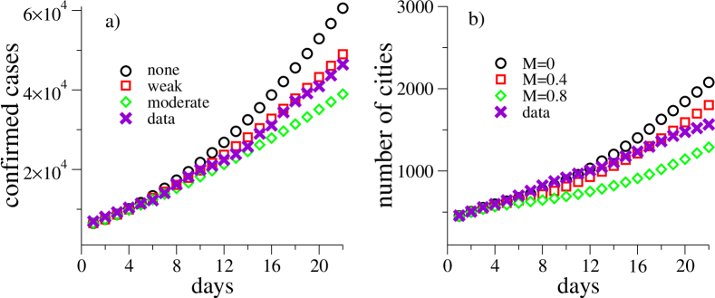
Figure 2: Comparison of simulations with reported data for COVID-19 in Brazil Cota (2020) for the first three weeks with day 0 corresponding to 31 March 2020. a) Number of confirmed cases are presented for different mitigation scenarios: none with $(M,K)=(0,0)$, weak with $(M,K)=(0.4,0.3)$ and moderate with $(M,K)=(0.8,0.5)$. b) Evolution of the number of municipalities with confirmed cases for a reduction of contact of $K=0.3$ and different levels of long distance mobility given by $M=0,~{}0.4$, and $0.8$.

II.5 Mitigation strategies

Different mitigation strategies are studied by uniformly reducing the inter-patch mobility and contact by factors $(M,K)$, i.e., $W_{ij}\rightarrow(1-M)W_{ij}$, for $j\neq i$, and $k_{i}\rightarrow(1-K)k_{i}$. We investigate three different scenarios: none, weak, and moderate mitigations represented by $(M,K)=(0,0)$, $(0.4,0.3)$, and $(0.8,0.5)$, respectively. We do not tackle the regime of suppression or strong mitigation that could drop the epidemic drastically. Averages were evaluated over 10 independent simulations.

II.6 Remarks on parameter choices

The extensive set of parameters is aimed to reproduce the essence of the epidemic spreading at a countrywide level but not to track accurately the epidemic outbreak in every state or municipality. We specially assume uniform and constant control parameters for reduction of inter-municipality movement and contacts as well as the testing rates. This is surely not the real case. Each federative state or municipality has its own mitigation and testing policies that are very heterogeneous. So, assuming uniformity and fitting the overall data at a country level, it is possible to infer in which regions the epidemic is evolving faster or slower than the average. Finally, our initial condition is a guess driven by data but still limited. The level of underreporting is known to be high, and broad ranges of values have been reported Li et al. (2020b); Bendavid et al. (2020); Hallal et al. (2020). The description of the complete set of epidemiological parameters, the initial conditions, mobility and demographic data are given in Appendix B.

III Nowcasting and model calibration

Irrespective of the heterogeneous testing approaches among states Cota (2020), we assume that essentially all municipalities had capacity to detect COVID-19 in the first hospitalized patients and, therefore, the number of municipalities with positive cases is expected to be an observable much less prone to the effects of underreporting than the number of confirmed cases at the beginning of the pandemics in Brazil. Figure 3 compares the evolution of municipalities with confirmed cases between 1 and 22 April 2020 obtained in simulations with different mitigation measures and real data for each Brazilian state and also for the whole country. Weak mitigation provides the best agreement with the reported data whereas deviations start to appear after three weeks. The weak mitigation parameters $(M,K)=(0.4,0.3)$, which fit better the overall data for Brazil, also perform well for most of the states in this time window and especially those with higher incidence of COVID-19 in the period, which lead the averages over the country. However, some states (AC, AM, PA, PE, PI, and RR - abbreviations for Brazilian federative states are given in Fig. 3) were more consistent with the simulations without mitigation while others (PB, PR, and RN) were nearer to a moderate mitigation. No tuning with respect to specific places was used and, consequently, it does not reproduce accurately the number of reported cases for all federative states due to the diversified testing and social distancing policies across different states and municipalities, in contrast with the uniformity hypothesis of the present study.

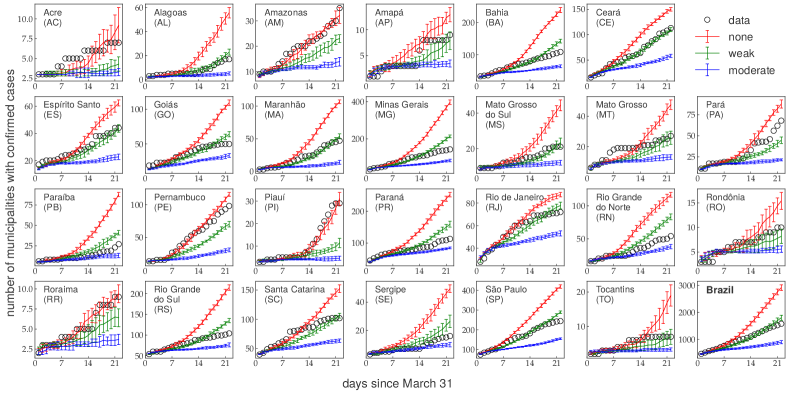
Figure 3: Simulations and observations of the number of municipalities with confirmed cases of COVID-19 for the 26 federative states of Brazil in the first three weeks of simulations. Data for the whole country are shown in the bottom right corner. Simulations were performed using none, weak, and moderate mitigations with parameters $(M,K)=(0,0),~{}(0.4,0.3)$, and $(0.8,0.5)$, respectively.

IV Geographical analysis of epidemic prevalence

The role of inter-municipality traffic is investigated reducing the contacts by 30% and varying the mobility. The total number of cases changes very little since the leading contribution comes from local transmission in municipalities with larger incidence while the number of municipalities with confirmed cases, shown in Fig. 2b), depends significantly on the inter-municipality traffic restrictions. These results confirm the epidemiological concept that reducing long-distance travelling contributes to delaying the outbreak onset in different places, but alters little the countrywide epidemic prevalence Colizza et al. (2007b), as discussed in the context of COVID-19 spreading in China Chinazzi et al. (2020); Du et al. (2020) and Spain Aleta and Moreno (2020), for example.

From now on, generic predictions under the aforementioned hypothetical scenarios are discussed. We stress that these predictions, whose time window spans after the resubmission time, were simulated in April 2020 Costa et al. (2020). High variability of the epidemic outbreaks (intensity, duration and delays) can be observed through all geographical scales. Diversity was found in other metapopulation approaches for epidemic processes Danon et al. (2009, 2020) but the multi-scale dispersion in our simulations is remarkable. At the state level, the time when the outbreak reaches its maximum epidemic prevalence, the epidemic peak, varies considerably as shown in Figs. 4a) and 4b), where the epidemic prevalences for all states are shown as function of time for a weak mitigation.

Let $T$ and $\rho$ be the time and prevalence of the epidemic peak , considering both unconfirmed and confirmed individuals. According to the simulations with weak mitigation, the first state to reach the peak would be CE ($T_{\text{CE}}\approx 34$ d), followed closely by SP and AM ($T_{\text{SP}}\approx T_{\text{AM}}\approx 36$ d). The respective prevalences would be $\rho_{\text{CE}}\approx 3.6\%$, $\rho_{\text{SP}}\approx 4.9\%$, and $\rho_{\text{AM}}\approx 5.0\%$. The state with highest epidemic prevalence would be RJ with $\rho_{\text{RJ}}\approx 7.0\%$ at $T_{\text{RJ}}\approx 40$ d. The epidemic peak would happen later ($T_{\text{MA}}=71$ d), with maximum less intense ($\rho_{\text{MA}}\approx 2.3$%) and the curve broader for the MA state. The MA case is particularly interesting because whereas the peak for the state would happen last, for its capital city São Luis it would occurs at day 41 slightly earlier than the average peak for Brazil, which would be at day $44$ in this scenario. These numbers should not be quantitatively compared with the real reported cases. Firstly, the confirmed cases correspond to a small fraction of the total of cases that depends on testing rate, an unknown variable in our study, and curves for $\rho_{\text{C}}$ are much broader and have the peak postponed to later times. Secondly, the uniform and constant mitigation and testing scenarios do not correspond to reality.

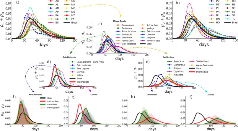
Figure 4: Multi-scale analysis of epidemic prevalence at several scales of geographical organization, considering a weak mitigation with parameters $(M,K)=(0.4,0.3)$. Epidemic curves averaged with geographical resolution increasing from top to bottom are compared with lower resolution averages: a,b) States, c) intermediate regions, d,e) immediate regions, f-i) municipalities. The curves presenting the earliest and latest maxima are chosen as representative within each panel c) to e). Arrows indicate curves selected for zooming. Day 0 corresponds to 31 March 2020. The state of MG was chosen for the higher resolution curves.

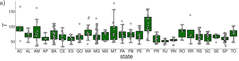
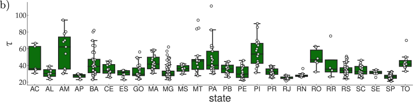
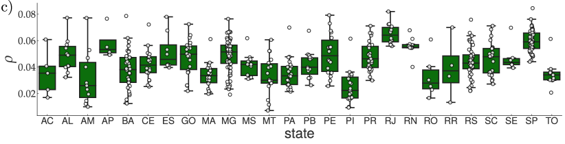
Figure 5: Box plots for the peak a) time $T$, b) width $\tau$, and c) prevalence $\rho$ averaged over immediate regions for the 26 federative states using a weak mitigation with parameters $(M,K)=(0.4,0.3)$. Circles are data for different regions. As usual, boxes yield median, lower and upper quartiles while points outside whiskers are outliers.

A spatially more refined analysis is done comparing immediate and intermediate geographical regions of a same federative state, which are determined by the Instituto Brasileiro de Geografia e Estatística (IBGE) Instituto Brasileiro de Geografia e Estatística (2017) (IBGE). An immediate region is a structure of nearby urban areas with intense interchange for immediate needs such as purchasing of goods, search for work, health care, and education. An intermediate region agglomerates immediate regions preferentially with the inclusion of large metropolitan areas Instituto Brasileiro de Geografia e Estatística (2017) (IBGE) laying thus between immediate regions and federative states. In Brazil there are 133 intermediate and 510 immediate regions. Municipalities in different federative states do not belong to the same immediate regions even if they have strong ties. The broad variability of epidemic outbreaks observed at the federative state level is repeated at higher resolutions of geographical aggregation. Figures 4c) to i) show the multi-scale structure of the outbreaks within the state of MG. They compare the epidemic prevalences of different intermediate regions, followed by the next scale with all immediate regions belonging to the pair of intermediate ones presenting the epidemic peak first and last in Figs. 4d) and e). Finally, the highest resolution with curves for municipalities within the respective immediate regions with the earliest and latest maxima are shown in Figs. 4f) to i).

A large dispersion through the 13 intermediate regions of the MG state is seen in Fig. 4c). The times and prevalence values at the peak differ by factors 2 and 6, respectively, between the regions that attain the maximum first and last. Curves for all intermediate regions of the 26 federative states are shown in Figs. S1, S2, and S3 of the SM sup for distinct mitigation strategies, showing that the more intense the mitigation the more heterogeneous are the curves across the country. Stepping down to immediate regions, a similar behavior is found in Figs. 4d) and e). The intermediate and immediate regions of Belo Horizonte, that include the capital city and are by far the most populous regions of this state, lead the averages over state and intermediate regions, respectively, blurring the actual prevalence in other localities. Variability is still large within immediate regions as shown in Figs. 4f) to i) with the epidemic prevalence (shaded plots) at different municipalities of a same immediate region. This pattern is repeated for other federative states: only the dispersion amplitude varies. This multi-scale nature for CE, RJ, RS, and SP states are respectively provided in Figs. S4, S5, S6, and S7 of the SM sup .

Variability of time, prevalence, and width $\tau$ (outbreak duration) of the epidemic peak throughout immediate regions are shown in the box plots of Fig. 5 for simulations with a weak mitigation. Box plots for none and moderate mitigations are qualitatively similar and presented in Figs. S8 and S9 of the SM sup . One can see that federative states with smaller territorial areas, such as SE, RN, and RJ, tend to have smaller dispersions of the peak time while those with larger and more sparsely connected territories, as AM, MT, and MS, have larger dispersions and outliers. We also have states with larger but better connected territories such as SP, PR, and RS, for which the dispersion is significant but not characterized by outliers. Irrespective of the more cohesive outbreak patterns, the epidemic peaks in immediate regions of the SP state, for example, could take more than twice as long as the peak at the capital city. Conversely, the outbreaks in the RJ state would be less desynchronized than in its neighbors, MG and SP, with the latest immediate region reaching the epidemic peak only 50% later than the capital city Rio de Janeiro, in this scenario.

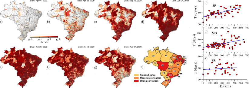
Figure 6: a-g) Color maps presenting the evolution of the prevalence of symptomatic cases (U and C) for Brazil in a simulation with a weak mitigation using parameters $(M,K)=(0.4,0.3)$. Dates of the simulation are shown in the upper right corner of each frame. The darker colors represent higher prevalences in a logarithm scale. h) Map with the classification of typical correlation between peak time $T$ and distance of immediate regions to capital cities $D$ of each federative state. See main text for criteria. Scatter plots of $T$ versus $D$ for the i) SP, j) MG and, k) PR states.

The space-time progression of the epidemic presents complex patterns as shown in Figure 6a) to g), where color maps with the prevalences of symptomatic cases in each municipality of Brazil are shown with intervals of three weeks for simulations using weak mitigation; see Figs. S10, and S11 of the SM sup for other scenarios. Full evolutions for all investigated mitigation parameters are provided in Movies S1, S2, and S3 of the SM sup . Epidemic waves propagating on average from the coast at east, where the most populated regions are, to inland can be seen at a country level. Moreover, when the epidemic is losing strength in the coast, the inland regions are still facing high levels of epidemic prevalence. Maps and movies suggest that the epidemic starts in the more populated places, usually the largest metropolitan regions, and spreads out towards the countryside. This is quite clear in the SP state, where the focus begins in its capital city and moves westward into the countryside. However, other states as PR and RS follow a different pattern with multiple foci evolving simultaneously.

We analyzed the correlation between time $T$ of the epidemic peak in the prevalence curves of immediate regions and their distances $D$ from the capital city of the respective state. Figures 6i)-k) show scatter plots of $D$ vs $T$ for three typical correlation patterns found in the simulations. The remaining states are given in Fig. S12 of the SM sup . The SP state presents a strong correlation with Pearson coefficient $r=0.69,$ statistically significant with $p$-value less than $10^{-7}$. For PR, no statistical correlation is observed. Finally, MG has a moderate correlation with Pearson coefficient $r=0.47$, but statistically significant with $p$-value of $10^{-5}$. We classified the states according to the correlation between $T$ and $D$ in three groups: not significant for which the $p$-value is larger than $0.02$; strong correlation that has statistical significance with $p<0.02$ and $r>0.6$; and moderate correlation with $p<0.02$ and $r<0.6$. The results are summarized in Fig. 6h) where the map shows states colored according to their classification. The structure does not change for other mitigation approaches. The complete set of Pearson coefficients and $p$-values are given in Fig. S12 of the SM sup . States in the north (RR, RO, AP, AC, AM, PA, and TO) have few immediate regions distributed in large territories and are less connected. Thus, lack of correlations is not surprising. Moderate correlations in states as MG, BA, and GO, with large but better connected territories are due to the existence of multiple important regions that play the role of regional capitals. However, PR is an extreme case with many and well connected immediate regions but total lack of correlations with the capital city, Curitiba.

V Discussion

The wide territorial, demographic, infrastructural diversities of large countries as Brazil demand modeling of a pandemic with geographical resolution higher than the usual compartmental epidemic models, which can be achieved using the metapopulation framework. We developed a stochastic metapopulation model and applied it to the COVID-19 spreading in Brazilian municipalities. Performing simulations with different hypothetical mitigation scenarios and considering the integration of regions through inter-municipality recurrent mobility, we have identified a high degree of heterogeneity and desynchronization of the epidemic curves between the main metropolitan areas and other inland regions. The diversity of outcomes is observed in several geographical scales, ranging from states to immediate regions, that enclose groups of nearby municipalities with strong economic and social ties. The intenser the mitigation attitudes, the more remarkable are the differences. Moderate or strong correlations between the delay of the epidemic peak in the interior regions and distance to the capital cities of the respective state were observed for most states with well connected immediate regions. However, one exception was the PR state where there are diverse epidemic foci evolving apparently independently of its capital city.

Our simulations suggest that uniform mitigation measures are not the optimal strategy. In a municipality where the peak without interventions would happen quite later than the capital city of its state, it would delay even more if strong mitigation measures are adopted synchronously with the capital. Nevertheless, such a place probably would have to extend the mitigation for much longer periods since once the epicenters of epidemics start to relax their restrictions, the viruses will circulate fast, reaching these vulnerable municipalities with most of population still susceptible. This is the actual current situation in Brazil at moment of resubmission. The social and economic impacts could be higher. On the other hand, an eventual collapse of the local heath system, a central question of the COVID-19 pandemic combating Arenas et al. (2020b), in the countryside regions could also occur after the larger metropolitan areas were under control, raising the possibility of unburdening the local healthy care system. In fact, the desynchronization of the epidemic curves and consequently of the health-system collapse could be an asset in designing optimal resource allocations. One could prevent rapid expansion of the epidemic through smaller municipalities flattening the curves as much as possible in the main metropolitan regions. Beyond the positive consequences for their own health systems, this attitude would have the positive side effect of delaying outbreaks in the countryside. Our study shows that countryside regions are not safe in the medium-term but could have precious additional time to prepare themselves.

VI Afterwords

There is an interval of five months between conceiving the first version of the present work Costa et al. (2020) and this final submission. As emphasized throughout the paper, our aim was to simulate hypothetical scenarios rather to do an accurate forecasting of real epidemic curves. Therefore, qualitative behaviors predicted in the simulations can now be confronted with the real series observed a posteriori. Several qualitative aspects predicted in simulations were indeed observed in real data. Maybe the most remarkable one is the confirmation of the multi-scale nature of the epidemic curves presented in Fig. 4 of the main text and Figs. S4 to S7 of SM sup . Figure 7 presents the epidemic incidences (new cases per capita over a week) for intermediate regions of three states presenting typical behaviors observed in simulations. The scenario of propagation starting from east coast towards inland, with a considerable delay for the epidemic peak in the latter, shown in Fig. 6 was also observed. Other interesting phenomena were also verified in real data as, for example, the unusual curve for the MA state and the multifocal spreading in some states as PR, MG and GO.

Lets consider in more details the SP state shown in Fig 7a), the one with highest number of COVID-19 cases in Brazil. One can see a moderate dispersion for peak occurrence time while in the capital city São Paulo it happened considerably earlier. This picture is the same drawn in Fig. S7a) of the SM sup . For the state of RJ, shown in Fig. 7b), the real data, with an exception for the intermediate region of Petropólis, are remarkably similar to simulations (see Fig. S5a) of the SM sup ), where intermediate regions peaks approximately synchronously with the intermediate region of Rio de Janeiro. We are not able to provide a specific reason for the different behavior of Petropólis. The incidence curves for the CE state, one of the first and more intensely impacted places by COVID-19 in Brazil and shown in Fig. 7c), are remarkably heterogeneous with Fortaleza reaching the maximum much earlier and Cretéus much later than the other intermediate regions. The incidence curve for the whole CE state is very broad meaning that different regions rule the state’ curve at different times, a scenario in almost perfect consonance with the simulation predictions shown in Fig. S4 of SM sup . We can also see significant dispersion for immediate regions’ curves within a same intermediate region, as illustrated for Sobral in Fig. 7d). Intermediate region of Cretéus is composed only by two intermediate regions and does not illustrate the point as well as Sobral does. The maximum incidence also varied considerably as, once more, predicted in simulations.

Quantitatively, a hypothetical scenario fitting better more regions lies between weak and moderate mitigations. However, as one could guess, different hypothetical scenarios works better at distinct moments and places confirming that quantitative forecasting and even nowcasting is a very dedicated issue.

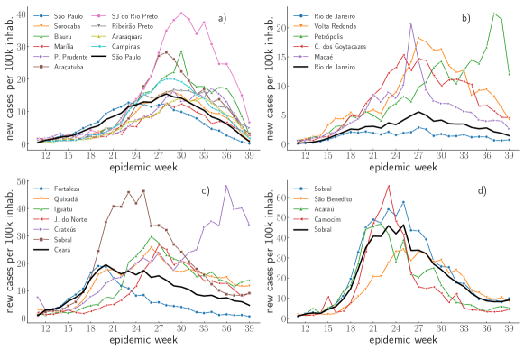
Figure 7: Real time series of epidemic incidence per week for intermediate regions of the states of a) SP, b) RJ, and c) CE and for the d) immediate regions belonging to the intermediate region of Sobral in the state of CE. Thick lines are the incidence for lower resolution scale in the corresponding a)-c) state or d) intermediate region. Data reported by onset of symptoms were extracted from e-SUS NOTIFICA official dataset held by Brazilian Ministry of Health Ministério da Saúde do Brasil (2020). Epidemic week 12 correspond to March 15-21, 2020.

Appendix A Computer implementation

The computer implementation of the epidemic model follows the Gillespie methods based on Ref. Cota and Ferreira (2017).

Definitions. We define $n^{\text{X}}_{ji}$ as the number of individuals in state X (= S,E,A,U,C, or R) within the patch $i$ that comes from patch $j$ such that $\tilde{n}^{\text{X}}_{i}=\sum_{j}n^{\text{X}}_{ji}$ is the number of individuals in patch $i$ that are in state X. Thus, the number of residents of $i$ in state X at patch $i$ is $n^{\text{X}}_{ii}$ and of nonresidents is given by $\tilde{n}^{\text{X}}_{i}-n^{\text{X}}_{ii}$. Also, $\tilde{n}_{i}=\sum_{X}\tilde{n}^{\text{X}}_{i}$ is the total number of individuals and $\tilde{n}_{ii}=\sum_{X}\tilde{n}^{\text{X}}_{ii}$ the number of residents in the patch $i$. Finally, the total number of individuals in the compartment X is $N_{\text{X}}=\sum_{j=1}^{\Omega}\tilde{n}^{\text{X}}_{i}$.

We have that $W_{ii}=N_{i}-\sum_{j\neq i}W_{ij}$ is the population of patch $i$ that does not leave it. The population fraction moving recurrently from $i$ to $j$ is

$$R_{ij}=\frac{W_{ij}}{\sum_{l}W_{il}}.$$ (5)

Thus, $R_{i}=\sum_{j\neq i}R_{ij}$ and $R_{ii}=1-R_{i}$ are, respectively, the population fractions that move or not from patch $i$.

General structure of the simulation. We divide the simulation in two big groups: mobility and epidemic events. The total rate of inter-patch mobility is

$$D_{\text{tot}}=T_{\text{r}}^{-1}\sum_{i}\tilde{n}_{ii}R_{i}+T_{\text{r}}^{-1}\sum_{i}(\tilde{n}_{i}-\tilde{n}_{ii}),$$ (6)

in which the first term represents the individuals leaving from and the second returning to their patches of residence.

The epidemic transitions $\mathcal{T}$ and their respective total rates $\Gamma_{\mathcal{T}}$ are defined in Table 1.

Table 1: Total transition rates for different types of epidemic events.

$\mathcal{T}$		$\Gamma_{\mathcal{T}}$		$\mathcal{T}$		$\Gamma_{\mathcal{T}}$
E$\rightarrow$A		$\mu_{\text{A}}N^{\text{E}}$		A$\rightarrow$U		$\beta_{\text{U}}N^{\text{A}}$
A$\rightarrow$R		$\beta_{\text{R}}N^{\text{A}}$		U$\rightarrow$R		$\alpha_{\text{R}}N^{\text{U}}$
U$\rightarrow$C		$\alpha_{\text{C}}N^{\text{U}}$		C$\rightarrow$R		$\alpha_{\text{R}}N^{\text{C}}$
S$\rightarrow$E		$\sum_{i=1}^{\Omega}\Theta_{i}$

The infection rate in a patch $i$ is given by

$$\Theta_{i}=\dfrac{k_{i}\tilde{n}^{\text{S}}_{i}}{\tilde{n}_{i}}\left(\lambda_{\text{A}}\tilde{n}^{\text{A}}_{i}+\lambda_{\text{U}}\tilde{n}^{\text{U}}_{i}+b\lambda_{\text{C}}\tilde{n}^{\text{C}}_{i}\right),$$ (7)

while the total rate of epidemic events is $E_{\text{tot}}=\sum_{\mathcal{T}}\Gamma_{\mathcal{T}}.$ In each time step, we select one mobility or epidemic event with probabilities $P_{\text{mob}}=D_{\text{tot}}/(D_{\text{tot}}+E_{\text{tot}})$ and $P_{\text{epi}}=1-P_{\text{mob}}$, respectively, and the time is increased by $\delta t=-\langle{\delta t}\rangle\ln\eta$ where $\langle{\delta t}\rangle=1/(D_{\text{tot}}+E_{\text{tot}})$ and $\eta$ is a pseudo random number uniformly distributed in the interval (0,1].

Inter-patch mobility events. If a mobility event was chosen we proceed as follows.

• Choose the patch $i$ from where an individual will leave proportionally to the total mobility rate of the patch, which occurs with probability

  $$Q_{i}=\frac{\tilde{n}_{ii}R_{i}+(\tilde{n}_{i}-\tilde{n}_{ii})}{\sum_{j}\left[\tilde{n}_{jj}R_{j}+(\tilde{n}_{j}-\tilde{n}_{jj})\right]}$$ (8)

• Choose the state X of the individual of patch $i$ that will move with probability

  $$P_{i}^{\text{X}}=\frac{\tilde{n}_{i}^{\text{X}}}{\sum_{\text{Y}}\tilde{n}_{i}^{\text{Y}}}.$$ (9)

• Select if the individual to move is resident or nonresident with probabilities $n^{\text{X}}_{ii}/\tilde{n}^{\text{X}}_{i}$ and $1-n^{\text{X}}_{ii}/\tilde{n}^{\text{X}}_{i}$, respectively.

• If the individual is resident and not symptomatic (S,E,A or R), the destination patch $j$ is chosen with probability $R_{ij}/\tilde{R}_{i}$. If he/she is symptomatic, stays in the resident patch ($j=i$). The movement is implemented as $n^{\text{X}}_{ij}\rightarrow n^{\text{X}}_{ij}+1$ and $n^{\text{X}}_{ii}\rightarrow n^{\text{X}}_{ii}-1$.

• If the individual to move is a nonresident, one patch $j$ is chosen with probability $n_{ji}^{\text{X}}/(\tilde{n}_{i}^{\text{X}}-\tilde{n}_{ii}^{\text{X}})$ and the movement is implemented as $n_{ji}^{\text{X}}\rightarrow n_{ji}^{\text{X}}-1$ and $n_{jj}^{\text{X}}\rightarrow n_{jj}^{\text{X}}+1$.

Epidemic events. If an epidemic event was chosen we proceed as follows.

• One of the transitions $\mathcal{T}$ is chosen with probability

  $$P_{\mathcal{T}}=\frac{\Gamma_{\mathcal{T}}}{\sum_{\mathcal{T}}\Gamma_{\mathcal{T}}}.$$ (10)

• If $\mathcal{T}=$ S$\rightarrow$E, then we choose a patch $i$ with probability $\Theta_{i}/\sum_{j=1}^{\Omega}\Theta_{j}$. Then, one patch $j$ is chosen with probability $n^{\text{S}}_{ji}/\tilde{n}^{\text{S}}_{i}$ and the populations are updated as $n^{\text{S}}_{ji}\rightarrow n^{\text{S}}_{ji}-1$ and $n^{\text{E}}_{ji}\rightarrow n^{\text{E}}_{ji}+1$. Notice that both resident ($i=j$) or nonresident ($i\neq j$) are considered in this rule.

• If $\mathcal{T}$ is a spontaneous transition of the form X$\rightarrow$Y then a patch $i$ is chosen with probability $\tilde{n}^{\text{X}}_{i}/N^{\text{X}}$ and the patch $j$ of residence is chosen with probability $n^{\text{X}}_{ji}/\tilde{n}^{\text{X}}_{i}$. Then $n^{\text{X}}_{ji}\rightarrow n^{\text{X}}_{ji}-1$ and $n^{\text{Y}}_{ji}\rightarrow n^{\text{Y}}_{ji}+1$.

This algorithm spends too much time with mobility of susceptible and removed individuals since they can exist in very large number for long times. We implemented an optimization performing the mobility of susceptible and removed in discrete times of $0.5~{}$d. So, instead of moving one susceptible individual at a time step, we move $n_{ii}^{\text{S}}R_{ij}$ from $i$ to $j$ at once and those who were not infected while visiting patch $j$, return to $i$ after $0.5~{}$d. The same is done for removed individuals. The simulations yield the same results as the exact procedure within the statistical uncertainties.

Appendix B Parameters for a data-driven approach

Mobility. Mobility parameters were extracted from public sources. Local commuting $C_{ij}^{(1)}$ was estimated from the national census data of 2010 provided by IBGE Instituto Brasileiro de Geografia e Estatística (2012) (IBGE) as the number of people that daily commute among municipalities to work or study. We excluded from the dataset those travels corresponding to more than 250 km, which are reckoned by airline travel data. Commuting data lacking destinations were included, assuming proportionality to the complete-information portion of the dataset; see Lana et al. (2017) for details. For the sake of generality, the recurrent flux is a function $W_{ij}^{(1)}=F_{ij}(C_{ij}^{(1)})$. We use the simplest case $F_{ij}(x)=x$. Air transportation data were obtained from the Agência Nacional de Aviação Civil (ANAC) Agência Nacional de Aviação Civil (2019) (ANAC) with the statistics of direct flights of 2014 considering the main nearby metropolitan region as the origin and destination of passengers. Using boarding and landing statistics of passengers, one-connection flights were inferred and the number of passengers $C_{ij}^{(2)}$ flying daily from $i$ to $j$ was estimated Coelho et al. (2020). In order to construct a recurrent mobility with flights, we assume $W_{ij}^{(2)}=(C_{ij}^{(2)}+C_{ji}^{(2)})/2$, which represents an effective flux. We do not have estimates for duration of long-range travels. However, this does not affect the current model since the homogeneous mixing hypothesis within the patches means that only the number of individuals that stay part of the time in two different patches actually matters and not who traveled. The total recurrent mobility is $W_{ij}=W_{ij}^{(1)}+W_{ij}^{(2)}$; we assume that it occurs daily, i.e, $T_{\text{r}}=1$ d since both commuting and air travel data were obtained with this time resolution.

Epidemiological parameters. We used epidemiological parameters based on Ref. Arenas et al. (2020b) which were mined from analyses of early COVID-19 epidemic spreading on Hubei province China Li et al. (2020a); Danon et al. (2020); Read et al. (2020). The total time in the exposed and asymptomatic compartments was taken as $\mu_{\text{A}}^{-1}+\beta_{\text{U}}^{-1}=5.2~{}\text{d}$ Li et al. (2020a). We used $\mu_{\text{A}}^{-1}=\beta_{\text{U}}^{-1}=2.6$ d. The time for a symptomatic individual be removed was estimated as $\alpha_{R}^{-1}=3.2~{}\text{d}$ Read et al. (2020); Danon et al. (2020). For the truly asymptomatic individuals, we used the same recovering time of the presymptomatic ones, such that $\beta_{\text{R}}^{-1}=\beta_{\text{U}}^{-1}+\alpha^{-1}_{\text{R}}$. The infection rates $\lambda_{\text{C}}=\lambda_{\text{U}}=\lambda_{\text{A}}=0.06$ d^-1 Chinazzi et al. (2020); Pitzer et al. (2007); Arenas et al. (2020b) and average number of contacts $\langle{k}\rangle=13$ were estimated to reproduce the scaling of Brazilian very early exponential growth, $\sim\exp{(0.3t)}$, in reported cases of COVID-19; see Fig. S13 in the SM sup . These parameters provide an effective infection rate $\lambda\langle{k}\rangle=0.78$ that represents an optimistic estimate nearer to the lower bounds estimated in other studies of COVID-19 Read et al. (2020); Zhan et al. (2020); Arenas et al. (2020b); Danon et al. (2020). The contact of the individuals who were confirmed for COVID-19 was depleted to a fraction $b=0.3$ of their regular contacts. The confirmation rate $1/\alpha_{\text{C}}^{(0)}=10$ d was calibrated together with the initial conditions to fit the amplitude of confirmed case curves after 31 March 2020 and also the total number of municipalities with confirmed cases in a weak mitigation scenario. This is approximately twice the incubation time implying that symptomatic individuals may not be tested even if tests are available. Up to 23 April 2020, Brazil had performed less than $1400$ tests per million inhabitants Cota (2020). Assuming a time window of 35 d for testing, we have approximately $\zeta=1/40~{}000$ d^-1 per inhabitant. Due to the testing targeted only to severe cases of respiratory syndromes adopted in Brazil to the date of investigation, the transition from asymptomatic to confirmed was neglected setting $\beta_{\text{C}}=0$; note that the model can easily include such a transition if the testing scenario changes.

Demographic parameters. Each patch represents a municipality with resident population given by IBGE using estimates of 2019 Instituto Brasileiro de Geografia e Estatística (2019) (IBGE), while the respective fractions of rural and urban populations were obtained from the IBGE census of 2010 Instituto Brasileiro de Geografia e Estatística (2012) (IBGE). The population density was determined using urban areas, obtained from high resolution satellite images, provided by Empresa Brasileira de Pesquisa Agropecuária (EMBRAPA) Farias et al. (2017). Both fraction and density of urban population, and, consequently, the number of contacts have broad distributions as can be seen in Fig. S13 of the SM sup . These are key features to enhance the accuracy of the predictions beyond large metropolitan centers. Parameter $a$ that controls the function $f(x)$ was taken as $a=1/\langle{\xi}\rangle$ where $\langle{\xi}\rangle=2791$ inhabitants/km² is the average urban population density of Brazil. The rural-urban contact matrix was chosen as $\mathcal{C}_{\text{uu}}=\mathcal{C}_{\text{rr}}=1$ and $\mathcal{C}_{\text{ru}}=0.5$. This last choice only assumes that urban-rural contacts are significantly smaller than urban-urban or rural-rural interactions.