Covariant formulation of gluon self-energy in presence of ellipsoidal anisotropy

Abstract

In this work, a covariant formulation of the gluon self-energy in presence of ellipsoidal anisotropy is considered. It is shown that the general structure of the gluon self-energy can be written in terms of six linearly independent projection tensors. Similar to the spheroidal anisotropy, mass scales can be introduced for each of the collective modes considering the static limits. With a simplified ellipsoidal generalization of the Romatschke-Strickland form, the angular dependencies of the mass scales are studied. It is observed that, compared to the spheroidal case, additional unstable mode may appear in presence of ellipsoidal anisotropy depending upon the choice of the parameters.

I Introduction

Over the last few decades, the plethora of knowledge gained through the nonperturbative lattice QCD simulations Ding:2015ona ; Ratti:2018ksb ; Bazavov:2019lgz , perturbative hard thermal loop calculations Braaten:1989mz ; Andersen:2004fp ; Haque:2014rua ; Su:2015esa , effective hydrodynamical modeling Gale:2013da ; Jeon:2015dfa ; Jaiswal:2016hex as well as AdS/CFT inspired studies Son:2007vk ; Nastase:2007kj ; Peschanski:2008xn ; Sadeghi:2013zma have paved the way of achieving a remarkable advancement in our understanding of the experimental data available from the Relativistic Heavy Ion Collider (RHIC) facility at Brookhaven National Lab and the Large Hadron Collider (LHC) facility at European Center for Nuclear Research (CERN)Stock:2010hoa ; Busza:2018rrf . The concerted efforts from different heavy ion research communities suggest that the deconfined quark-gluon plasma(QGP) matter produced in the ultrarelativistic heavy ion collision experiments is most likely to possess substantial deviation from perfect local isotropic equilibrium Strickland:2013uga . In fact, soon after the initial nuclear impact, very large pressure anisotropy is expected in the center of the fireball with even larger anisotropy prevailing in the cooler regions of the plasma Strickland:2014pga . A promising way for hydrodynamical modeling of such highly momentum space anisotropic system is to consider the framework of anisotropic hydrodynamics Alqahtani:2017jwl ; Alqahtani:2017mhy . On the other hand, incorporating certain classes of anisotropic momentum distributions in the framework of hard thermal loop perturbation theory, the nonequilibrium plasma properties can be extracted by studying the collective modes of the quasipartons Mrowczynski:2004kv ; Mrowczynski:2000ed . A suitable parametrization for such distributions can be achieved following Refs. Romatschke:2003ms ; Romatschke:2004jh ; Schenke:2006fz where the one particle isotropic momentum space distribution function is deformed by introducing a directional dependency. This particular Romatschke-Strickland (RS) form has been widely used in different phenomenological applications such as photon and dilepton production from anisotropic QGP Bhattacharya:2008up ; Bhattacharya:2008mv ; Bhattacharya:2015ada , anisotropic heavy quark potential Nopoush:2017zbu , bottomonia suppression Krouppa:2016jcl , plasma wakes Mandal:2012wi ; Mandal:2013jla , nuclear modification factor Mandal:2011xn , quasiparticle descriptions of particle production Chandra:2016dwy and so on.

An important aspect of considering the nonequilibrium momentum distributions in QGP medium is the occurrence of kinetic instabilities. These are, in simple terms, the collective modes that possess a positive imaginary part in their mode frequencies resulting an exponential growth in the chromomagneic and chromoelectric fields. The existence of such Chromo-Weibel instabilities Strickland:2006cv can influence the thermalization and isotropization of the medium Rebhan:2004ur . A recent review with a pedagogical introduction to the required theoretical tools for such studies can be found in Ref. Mrowczynski:2016etf . In general, how many unstable modes are possible depends on the choice of the parameters. For example, in case of spheroidal anisotropy with Romatschke-Strickland parametrized form, the number of the possible unstable modes differs for the prolate and the oblate case which are obtained considering the negative and positive values for the anisotropy parameter respectively Romatschke:2003ms . Moreover, there will be a directional dependence as well. In other words, depending on the angle of propagation with respect to the anisotropy direction, a stable collective mode may become unstable and can give rise to additional instabilities.

As already mentioned, the large momentum space anisotropy in early stages can be efficiently incorporated in the aHydro framework. This is because, unlike usual viscous hydrodynamic set up, here, the dominant anisotropic contributions to the distribution functions are captured in the leading order of hydrodynamic expansion. The second order anisotropic hydrodynamics as developed in Bazow:2013ifa can take into account arbitrary transverse expansion and is consistent with the traditional dissipative hydrodynamics approach in the limiting case of small anisotropy. However, as argued in Ref. Tinti:2013vba , the azimuthally symmetric ansatz in such approaches involving a single anisotropy parameter can further be generalized in a systematic way. More specifically, in the original anisotropic hydrodynamic setup, the leading order local rest frame distribution is taken to be of RS form and thus the two components of the pressure in the transverse plane can be different only after including the second order corrections. A generalization to include three different pressure components in the leading order of hydrodynamic expansion has been developed in Refs. Tinti:2013vba ; Nopoush:2014pfa ; Alqahtani:2015qja and recently has further been generalized in Ref. Nopoush:2019vqc . In the hard loop approach too, the generalized ellipsoidal distribution has been considered in the parton self-energy studies Kasmaei:2016apv and implemented in phenomenological applications of photon and dilepton production Kasmaei:2019ofu ; Kasmaei:2018oag . Obviously, the consideration of an ellipsoidal anisotropy increases the number of parameters compared to the spheroidal case, as, apart from one additional anisotropy parameter dependence, the collective properties of the partons in this case also possess azimuthal angular dependency. Recently, the gluonic unstable mode with an ellipsoidal anisotropic momentum distribution has been reported for the first time in Ref. Kasmaei:2018yrr . It is observed that the growth rate of the unstable modes can become several times larger than the spheroidal case for certain propagation directions. Also the number of possible unstable modes are direction dependent. A convenient method to describe such directional dependency is to consider the static limits of the collective modes. In that case, one introduces mass scales corresponding to each of the collective modes and studies their angular dependency. The occurrence of a negative value in the mass scale in fact signifies the presence of an instability in the corresponding mode which are well studied in the spheroidal case. However, for the ellipsoidal case, such mass scales could not be defined in the formalism adopted in Kasmaei:2018yrr where the general structure of the gluon polarization has not been considered. An important application of gluon self energy lies in the determination of the perturbative part of the heavy quark potential Dumitru:2007hy ; Dumitru:2009fy ; Nopoush:2017zbu which requires a covariant formulation of the general structure.

The primary objective of this work is to formulate a general structure for the gluon polarization in presence of ellipsoidal momentum space anisotropy in a covariant way and study the occurrence of the unstable modes in a similar fashion as done in case of spheroidal momentum space anisotropy. A suitable approach for constructing the tensor basis for gluon self energy is to choose the maximum possible mutually orthogonal set. The choice becomes useful for the derivation of the effective propagator where contractions among the basis tensors are involved. Once the effective gluon propagator is derived, one can obtain the collective modes from its pole. It should be mentioned here that the gluon collective modes can also be obtained by solving the characteristic equation without requiring any consideration of the general structure. In fact, this is the procedure adopted in Ref.Kasmaei:2018yrr . However, the advantage of considering the general structure is that, the collective modes are expressed in terms of coordinate independent form factors which is essential for introducing the mass scales. In fact, the nontrivial angular dependence in the hard-thermal loop resummed potential enters through these mass scales Nopoush:2017zbu .

The article is organized as follows. We first describe the formalism for constructing the general structure for the gluon polarization function in presence of the ellipsoidal anisotropy. The derived structure is subsequently used to obtain the effective propagator and the collective modes of the gluon. Considering to a simple ellipsoidal generalization of the RS form, the numerical results for the form factors and the mass scales are presented in the following section. Finally we conclude with a brief summary of the presented work. The following convention is used throughout the article: metric $\eta^{\mu\nu}=\mbox{diag}(1,-1,-1,-1)$ and a general momentum four vector $Q^{\mu}=(q^{0},\bm{q})$ with $Q^{2}$ representing $\eta_{\mu\nu}Q^{\mu}Q^{\nu}=Q\cdot Q$ and $q=|{\bm{q}}|$.

II Formalism

We consider a thermal QCD medium with a general anisotropic momentum distribution characterized by two independent four vectors $a^{\mu}$ and $b^{\mu}$ having unit norms. These two, together with the normalized heat bath velocity ($u^{\mu}$) and the gluon momentum ($P^{\mu}$), can be used to form a set of ten independent symmetric tensors so that the symmetric gluon polarization tensor can be expressed as a linear combination of them. A simple choice for this purpose may be the set of tensors $P^{\mu}P^{\nu}$, $u^{\mu}u^{\nu}$, $b^{\mu}b^{\nu}$, $a^{\mu}a^{\nu}$, $P^{\mu}u^{\nu}+P^{\nu}u^{\mu}$, $P^{\mu}b^{\nu}+P^{\nu}b^{\mu}$, $P^{\mu}a^{\nu}+P^{\nu}a^{\mu}$, $u^{\mu}b^{\nu}+b^{\mu}u^{\nu}$, $u^{\mu}a^{\nu}+u^{\nu}a^{\mu}$ and $b^{\mu}a^{\nu}+a^{\mu}b^{\nu}$. Notice that, along with the four vectors, we have not considered the metric $\eta^{\mu\nu}$ as usually done in isotropic or even in anisotropic case with one anisotropy direction. This is because, in case of ellipsoidal anisotropy, the metric itself no longer remains an independent tensor and can be expressed as a linear combination of the chosen set. Now, the constraints from the transversality condition $P^{\mu}\Pi_{\mu\nu}=0$ further reduce the number of independent basis tensors to six. In the rest frame of the heat bath with $u^{\mu}=(1,0,0,0)$, one of the anisotropy directions can be taken along z, say $b^{\mu}=(0,0,0,1)$, whereas the other anisotropy direction can be assumed to lie in the $xz$ plane without any loss of generality. In the following we discuss a convenient method to obtain the basis tensors in a systematic way.

Let us first consider the general structure of the gauge boson self-energy in vacuum that can be written as

$$\Pi^{\mu\nu}=\left(\eta^{\mu\nu}-\frac{P^{\mu}P^{\nu}}{P^{2}}\right)\Pi(P^{2})=V^{\mu\nu}\Pi(P^{2}).$$ (1)

Using the tensor $V^{\mu\nu}$, we obtain $\tilde{u}^{\mu}=V^{\mu\nu}u_{\nu}$ which can be used to construct the first basis tensor given by

$$A^{\mu\nu}=\frac{\tilde{u}^{\mu}\tilde{u}^{\nu}}{\tilde{u}^{2}}.$$ (2)

Now, it is useful to define the $A^{\mu\nu}$ subtracted part of $V^{\mu\nu}$ as $U^{\mu\nu}=V^{\mu\nu}-A^{\mu\nu}$ which can be used to obtain $\tilde{b}^{\mu}$ defined as $\tilde{b}^{\mu}=U^{\mu\nu}b_{\nu}$ such that it becomes orthogonal to $\tilde{u}^{\mu}$ by construction. Similar to the earlier case, we obtain our second basis tensor using $\tilde{b}^{\mu}$ as

$$B^{\mu\nu}=\frac{\tilde{b}^{\mu}\tilde{b}^{\nu}}{\tilde{b}^{2}}.$$ (3)

Another symmetric tensor that can be constructed intuitively using $\tilde{b}^{\mu}$ and $\tilde{u}^{\mu}$ together is given by

$$C^{\mu\nu}=\frac{\tilde{u}^{\mu}\tilde{b}^{\nu}+\tilde{b}^{\mu}\tilde{u}^{\nu}}{\sqrt{\tilde{u}^{2}}\sqrt{\tilde{b}^{2}}}.$$ (4)

To obtain the rest of the tensors, once again we go through the similar steps: at first we define $R^{\mu\nu}=U^{\mu\nu}-B^{\mu\nu}$, which, in this case, can be viewed as the $A^{\mu\nu}$ and the $B^{\mu\nu}$ subtracted part of our vacuum basis tensor $V^{\mu\nu}$. Then we obtain the $\tilde{a}^{\mu}$ from $a^{\mu}$ as $\tilde{a}^{\mu}=R^{\mu\nu}a_{\nu}$. This time, the newly constructed $\tilde{a}^{\mu}$ becomes orthogonal to $\tilde{b}^{\mu}$ as well as $\tilde{u}^{\mu}$. Note that, all the four vectors of the set $\tilde{u}^{\mu}$, $\tilde{b}^{\mu}$ and $\tilde{a}^{\mu}$ are orthogonal to the gluon four momentum $P^{\mu}$ and hence the basis tensors constructed using them trivially satisfy the transversality condition. Moreover, because of the orthogonality among the constructed four vectors, the extraction of the form factors gets simplified considerably. Now, with the constructed set, the rest of the independent symmetric tensors can also be obtained intuitively as

$$D^{\mu\nu} = \frac{\tilde{a}^{\mu}\tilde{a}^{\nu}}{\tilde{a}^{2}},$$ (5)

$$E^{\mu\nu} = \frac{\tilde{u}^{\mu}\tilde{a}^{\nu}+\tilde{a}^{\mu}\tilde{u}^{\nu}}{\sqrt{\tilde{u}^{2}}\sqrt{\tilde{a}^{2}}},$$ (6)

$$F^{\mu\nu} = \frac{\tilde{a}^{\mu}\tilde{b}^{\nu}+\tilde{b}^{\mu}\tilde{a}^{\nu}}{\sqrt{\tilde{a}^{2}}\sqrt{\tilde{b}^{2}}}.$$ (7)

The general structure of the gauge boson self-energy in presence of an ellipsoidal anisotropic medium can be expressed as a linear combination of the six basis tensors as

$$\Pi^{\mu\nu} = \alpha A^{\mu\nu}+\beta B^{\mu\nu}+\gamma C^{\mu\nu}+\delta D^{\mu\nu}+\sigma E^{\mu\nu}+\lambda F^{\mu\nu}~{}.$$ (8)

It is worth mentioning here that though tensors like $V^{\mu\nu}$ are used to obtain the set, once we declare our constructed set of tensors as independent, all the other symmetric and transverse tensors not belonging to the set become expressible as their linear combination. For example, it can be shown that

$$V^{\mu\nu} = A^{\mu\nu}+B^{\mu\nu}+D^{\mu\nu}.$$ (9)

Now, we can obtain the effective propagator from the Dyson-Schwinger equation

$$i\mathcal{D}^{\mu\nu} = i\mathcal{D}_{0}^{\mu\nu}+i\mathcal{D}_{0}^{\mu\rho}(i\Pi_{\rho\rho^{\prime}})i\mathcal{D}^{\rho^{\prime}\nu},$$ (10)

where the inverse bare propagator $\mathcal{D}_{0}^{\mu\nu}$ without the explicit color indices is given by

$$(\mathcal{D}^{-1}_{0})^{\mu\nu} = -P^{2}\eta^{\mu\nu}-\frac{1-\zeta}{\zeta}P^{\mu}P^{\nu},$$ (11)

with $\zeta$ representing the gauge fixing parameter. To obtain the effective propagator, let us first consider the inner product identities among the basis tensors. To express the identities in a compact form, here we suppress the Lorentz indices of the basis tensors. Also the tensors $C$, $E$, and $F$ are considered as a sum of two parts, for example $C=\overline{C}+\underline{C}$ and in similar fashion for the other two where

$$\overline{C}_{\nu}^{\mu}=\frac{\tilde{u}^{\mu}\tilde{b}_{\nu}}{\sqrt{\tilde{u}^{2}}\sqrt{\tilde{b}^{2}}},\hskip 14.22636pt\underline{C}_{\nu}^{\mu}=\frac{\tilde{b}^{\mu}\tilde{u}_{\nu}}{\sqrt{\tilde{u}^{2}}\sqrt{\tilde{b}^{2}}},$$

$$\overline{E}_{\nu}^{\mu}=\frac{\tilde{u}^{\mu}\tilde{a}_{\nu}}{\sqrt{\tilde{u}^{2}}\sqrt{\tilde{a}^{2}}},\hskip 14.22636pt\underline{E}_{\nu}^{\mu}=\frac{\tilde{a}^{\mu}\tilde{u}_{\nu}}{\sqrt{\tilde{u}^{2}}\sqrt{\tilde{a}^{2}}},$$

$$\overline{F}_{\nu}^{\mu}=\frac{\tilde{a}^{\mu}\tilde{b}_{\nu}}{\sqrt{\tilde{a}^{2}}\sqrt{\tilde{b}^{2}}},\hskip 14.22636pt\underline{F}_{\nu}^{\mu}=\frac{\tilde{b}^{\mu}\tilde{a}_{\nu}}{\sqrt{\tilde{a}^{2}}\sqrt{\tilde{b}^{2}}}.$$

With this notation, the inner product between the basis tensors can be written in a compact form as

(19)

where the composition rule for each entry of the multiplication table is defined as $r^{\mu}_{\rho}c^{\rho}_{\nu}$ with $r$ and $c$ being members representing the row and the column respectively. Moreover, further contraction of the free indices as $r^{\mu}_{\rho}c^{\rho}_{\mu}$ simplifies to

(27)

which will be useful to extract the coefficients of the basis tensors, i.e., the form factors from the polarization function. Using the properties of the basis tensors from Eq. (19) one can obtain the effective gluon propagator given by

$$\mathcal{D}^{\mu\nu} = -\frac{\beta\delta-\left(\beta+\delta\right)P^{2}-\lambda^{2}+P^{4}}{\Delta}A^{\mu\nu}-\frac{\delta\alpha-\left(\delta+\alpha\right)P^{2}-\sigma^{2}+P^{4}}{\Delta}B^{\mu\nu}-\frac{\gamma\left(P^{2}-\delta\right)+\sigma\lambda}{\Delta}C^{\mu\nu}$$ (28)

$$- \frac{\alpha\beta-\left(\alpha+\beta\right)P^{2}-\gamma^{2}+P^{4}}{\Delta}D^{\mu\nu}-\frac{\sigma\left(P^{2}-\beta\right)+\lambda\gamma}{\Delta}E^{\mu\nu}-\frac{\lambda\left(P^{2}-\alpha\right)+\gamma\sigma}{\Delta}F^{\mu\nu}-\zeta\frac{P^{\mu}P^{\nu}}{P^{4}}.$$

where the common denominator of the basis tensors, $\Delta$ is given by

$$\Delta = P^{6}-(\alpha+\beta+\delta)P^{4}-(\gamma^{2}+\sigma^{2}+\lambda^{2}-\alpha\beta-\beta\delta-\delta\alpha)P^{2}+\alpha\lambda^{2}+\beta\sigma^{2}+\delta\gamma^{2}-\alpha\beta\delta-2\gamma\sigma\lambda.$$ (29)

Notice that, in presence of ellipsoidal anisotropy, the denominator of the effective propagator becomes a cubic equation of $P^{2}$ and can be written as a product of three factors as

$$\Delta = (P^{2}-\Omega_{0})(P^{2}-\Omega_{+})(P^{2}-\Omega_{-}),$$ (30)

where $\Omega_{0}$ and $\Omega_{\pm}$ can be written in terms of the form factors as

$$\Omega_{0} = \frac{1}{3}(\alpha+\beta+\delta)-\frac{1}{3}\frac{\varpi}{\Big{(}\frac{\chi+\sqrt{4\varpi^{3}+\chi^{2}}}{2}\Big{)}^{\frac{1}{3}}}+\frac{1}{3}\Big{(}\frac{\chi+\sqrt{4\varpi^{3}+\chi^{2}}}{2}\Big{)}^{\frac{1}{3}},$$ (31)

$$\Omega_{+} = \frac{1}{3}(\alpha+\beta+\delta)+\frac{1+i\sqrt{3}}{6}\frac{\varpi}{\Big{(}\frac{\chi+\sqrt{4\varpi^{3}+\chi^{2}}}{2}\Big{)}^{\frac{1}{3}}}-\frac{1-i\sqrt{3}}{6}\Big{(}\frac{\chi+\sqrt{4\varpi^{3}+\chi^{2}}}{2}\Big{)}^{\frac{1}{3}},$$ (32)

$$\Omega_{-} = \frac{1}{3}(\alpha+\beta+\delta)+\frac{1-i\sqrt{3}}{6}\frac{\varpi}{\Big{(}\frac{\chi+\sqrt{4\varpi^{3}+\chi^{2}}}{2}\Big{)}^{\frac{1}{3}}}-\frac{1+i\sqrt{3}}{6}\Big{(}\frac{\chi+\sqrt{4\varpi^{3}+\chi^{2}}}{2}\Big{)}^{\frac{1}{3}},$$ (33)

where $\varpi$ and $\chi$ are given by

$$\varpi = \alpha(\beta-\alpha)+\beta(\delta-\beta)+\delta(\alpha-\delta)-3(\gamma^{2}+\lambda^{2}+\sigma^{2}),$$ (34)

$$\chi = (2\alpha-\beta-\delta)(2\beta-\delta-\alpha)(2\delta-\alpha-\beta)+54\gamma\lambda\sigma$$ (35)

$$- 9\alpha(2\lambda^{2}-\sigma^{2}-\gamma^{2})-9\beta(2\sigma^{2}-\gamma^{2}-\lambda^{2})-9\delta(2\gamma^{2}-\lambda^{2}-\sigma^{2}).$$

Once the form factors are extracted from the polarization function, the desired collective modes of the gluon can be obtained from the pole of the effective propagator.

III Results

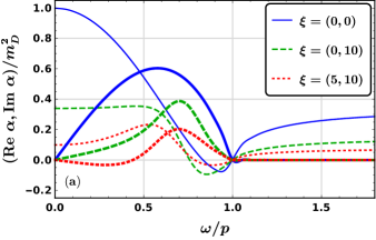
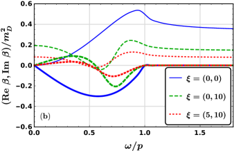
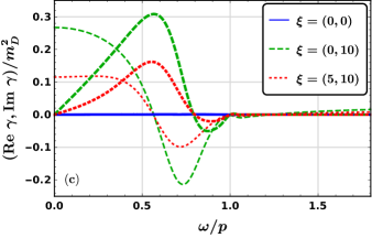
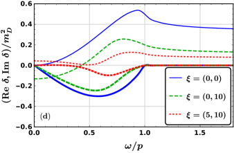
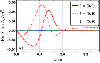
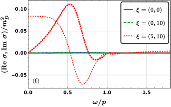
Figure 1: The real and imaginary parts of the form factors are plotted in (a)–(f) as a function of $\omega/p$ for three different sets of anistotropy tuple $\xi=(\xi_{a},\xi_{b})=(0,0),(0,10),$ and $(5,10)$. In each case, the imaginary parts are shown with comparatively thicker style. The spheroidal set is shown at fixed $\theta_{p}=\pi/4$ whereas for the ellipsoidal case, $(\theta_{p},\phi_{p})=(\pi/4,\pi/3)$ is considered.

In this work we consider the hard-loop gluon polarization tensor in a nonequilibrium QGP medium given by Mrowczynski:2000ed

$$\Pi^{\mu\nu}(p^{0}=\omega,{\bm{p}}) = g_{s}^{2}\int\frac{d^{3}{\bm{k}}}{(2\pi)^{3}}\frac{K^{\mu}}{E_{k}}\frac{\partial f({\bm{k}})}{\partial K^{\rho}}\Big{[}\eta^{\rho\nu}-\frac{K^{\rho}P^{\nu}}{P\cdot K+i0^{+}}\Big{]},$$ (36)

where $g_{s}$ is the strong coupling constant and $k^{0}=E_{k}$ represents the energy of the massless partonic degrees of freedom that modify the gluon dispersion in presence of anisotropic medium. The effective distribution function $f({\bm{k}})$ is given by

$$f({\bm{k}})=2N_{c}n_{g}({\bm{k}})+N_{f}\big{[}n_{q}({\bm{k}})+n_{\overline{q}}({\bm{k}})\big{]},$$ (37)

where $n_{g}({\bm{k}})$ represents the gluon number density whereas $n_{q}({\bm{k}})$ and $n_{\overline{q}}({\bm{k}})$ are the quark and antiquark number densities respectively. $N_{c}$ and $N_{f}$ are respectively the number of colors and quark flavors. A general method of constructing anisotropic momentum distribution function is to transform the argument of an isotropic momentum space distribution essentially by introducing deformations in a parametrized way. A discussion on the generalization of the RS form to ellipsoidal anisotropies can be found in Refs.Nopoush:2014pfa ; Kasmaei:2018yrr . In our case we use the ellipsoidal momentum distribution parametrized as Kasmaei:2016apv ; Kasmaei:2018yrr

$$f_{\mbox{aniso}}({\bm{k}})\equiv f_{\mbox{iso}}\big{(}\frac{1}{\Lambda}\sqrt{{\bm{k}}^{2}+\xi_{a}({\bm{k}}\cdot{\bm{a}})^{2}+\xi_{b}({\bm{k}}\cdot{\bm{b}})^{2}}\big{)},$$ (38)

where $\Lambda$ represents a temperature-like scale which, in the equilibrium limit, corresponds to the temperature. The gluon polarization tensor with such anisotropic parton distributions can be written as

$$\Pi^{\mu\nu}(\omega,{\bm{p}},\xi) = m_{D}^{2}\int\frac{d\Omega}{4\pi}v^{\mu}\frac{v^{l}+\xi_{a}({\bm{v}}\cdot{\bm{a}})a^{l}+\xi_{b}({\bm{v}}\cdot{\bm{b}})b^{l}}{(1+\xi_{a}({\bm{v}}\cdot{\bm{a}})^{2}+\xi_{b}({\bm{v}}\cdot{\bm{b}})^{2})^{2}}\Big{[}\eta^{\nu l}-\frac{v^{\nu}P^{l}}{\omega-{\bm{p}}\cdot{\bm{v}}+i0^{+}}\Big{]},$$ (39)

where $\xi$ represents the anisotropy tuple $(\xi_{a},\xi_{b})$ and $m_{D}^{2}=(N_{c}+N_{f}/2)\frac{g_{s}^{2}\Lambda^{2}}{3}$ corresponds to the QCD Debye mass scale. In the above expression, the parton four velocity $v^{\mu}=K^{\mu}/k$ and the components of ${\bm{a}}$, ${\bm{b}}$, ${\bm{v}}$, and ${\bm{p}}$ in the rest frame of the medium are chosen as

$${\bm{a}} = (1,0,0),$$ (40)

$${\bm{b}} = (0,0,1),$$ (41)

$${\bm{v}} = (\sin\theta_{k}\cos\phi_{k},\sin\theta_{k}\sin\phi_{k},\cos\theta_{k}),$$ (42)

$${\bm{p}} = p(\sin\theta_{p}\cos\phi_{p},\sin\theta_{p}\sin\phi_{p},\cos\theta_{p}),$$ (43)

with $d\Omega$ representing the differential solid angle corresponding to the internal angular coordinates $(\theta_{k},\phi_{k})$. It should be mentioned here that another common choice of reference frame is the parton specific coordinate as used in Ref. Kasmaei:2018yrr where one reorients the axes so that the polar angle is measured with respect to the parton momentum. However, as we are interested in the evaluation of the form factors, the results do not depend on any specific choice of the reference frame.

Now, as discussed in the previous section, the gluon self-energy can be decomposed in terms of six independent basis tensors. Utilizing the contraction relations among the basis tensors, the corresponding form factors can be obtained in terms of the self-energy components given in Eq.(39) as a two dimensional integral over the solid angle. However, because of the transversality condition and the symmetry under the exchange of the free indices, the number of independent components of the self-energy reduces to six. Thus, any chosen set of six independent components will be sufficient to determine the form factors. It should be mentioned here that, though in our work, the form factors are obtained numerically using the conventional quadrature routines, an alternative way involving the hypergeometric expansion method is expected to be much more efficient Kasmaei:2018yrr for this purpose. The real and imaginary parts of the form factors are shown in Fig. 1, for three different situations, namely the isotropic case with $\xi=(0,0)$, the spheroidal case with $\xi=(0,10)$ and the ellipsoidal case with $\xi=(5,10)$. The spheroidal case is shown for $\theta_{p}=\pi/4$ whereas for the ellipsoidal anisotropy, $\theta_{p}$ and $\phi_{p}$, are chosen as $\pi/4$ and $\pi/3$, respectively. The imaginary parts of the form factors in all the three cases exist only in the spacelike region. It should be noted that, when the isotropic medium is considered, $\beta$ and $\delta$ become degenerate whereas $\gamma$, $\lambda$, and $\sigma$ become zero. This results in two distinct dispersive modes of the gluon among which one is degenerate, i.e., $\Omega_{0}=\alpha$ and $\Omega_{+}=\Omega_{-}=\beta=\delta$. The analytic expression of the degenerate form factors is given by

$$\beta=\delta=\Pi_{T}=\frac{m_{D}^{2}}{2}\frac{\omega^{2}}{p^{2}}\bigg{[}1-\frac{\omega^{2}-p^{2}}{2\omega p}\ln\frac{\omega+p}{\omega-p}\bigg{]},$$ (44)

whereas the dispersion for the other distinct mode can be obtained from

$$\alpha=\Pi_{L}=\frac{m_{D}^{2}}{\tilde{u}^{2}}\bigg{[}1-\frac{\omega}{2p}\ln\frac{\omega+p}{\omega-p}\bigg{]},$$ (45)

which are the familiar results of the gluon self-energy in isotropic thermal medium Bellac:2011kqa . Here $m_{D}^{2}=(N_{c}+N_{f}/2)\frac{g_{s}^{2}T^{2}}{3}$ and $\tilde{u}^{2}=-p^{2}/P^{2}$. In the presence of spheroidal anisotropy, $\sigma$ and $\lambda$ remain zero. However, $\beta$ and $\delta$ are no longer degenerate. In that case the functions corresponding to the dispersive modes simplify to

$$\Omega_{0} = \frac{1}{2}\bigg{(}\alpha+\beta+\sqrt{(\alpha-\beta)^{2}+4\gamma^{2}}\bigg{)},$$ (46)

$$\Omega_{+} = \frac{1}{2}\bigg{(}\alpha+\beta-\sqrt{(\alpha-\beta)^{2}+4\gamma^{2}}\bigg{)},$$ (47)

$$\Omega_{-} = \delta.$$ (48)

which may be compared with the modes obtained in Ref. Romatschke:2003ms (see for example Eq.(43) therein). Though we find a different combination of the form factors in the expressions due to the different choice of our basis tensors, it should be noticed that, in our case too, the arguments inside the square root appear as a sum of two complete squares, thereby allowing similar interpretation for the collective modes [see for example Sec. VI of Romatschke:2003ms ]. When ellipsoidal anisotropy is considered, it is observed that all the form factors are nonzero and they contribute in the gluon dispersion. However, It should be noticed that, for the fixed set of parameters chosen for the figure, the values of $\lambda$ and $\sigma$ are an order of magnitude smaller than the other form factors.

Now, following Ref. Romatschke:2003ms , a mass scale corresponding to a given form factor, say for example $\alpha$, can be defined in the static limit as

$$m_{\alpha}^{2}=\lim_{\omega\rightarrow 0}\alpha.$$ (49)

It is evident from Fig. 1 that the imaginary part of each of the form factors vanishes at $\omega\rightarrow 0$ limit. Thus, the mass scales as defined above are real quantities. Now, in a similar way, one can define the mass scales corresponding to the gluon dispersive modes as

$$m_{\Omega_{0,\pm}}^{2}=\lim_{\omega\rightarrow 0}\Omega_{0,\pm}(\omega,p,\theta_{p},\phi_{p}).$$ (50)

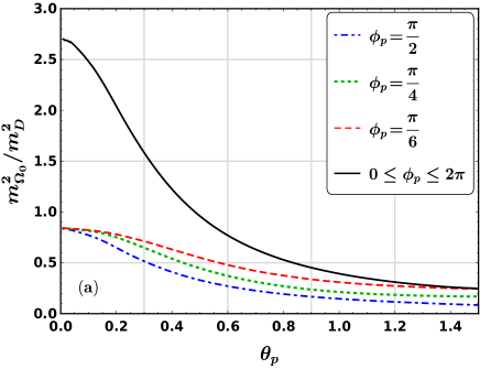
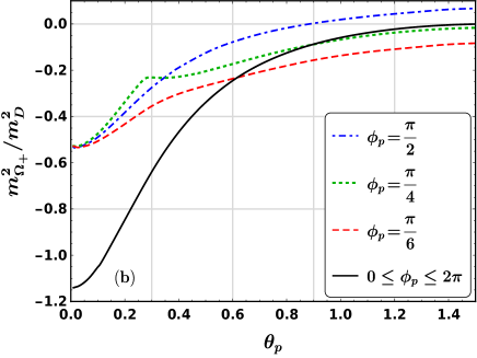
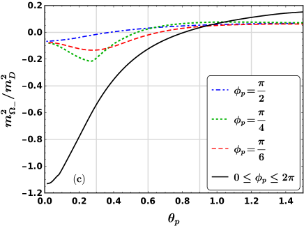
Figure 2: Squared values of the mass scales corresponding to $\Omega_{0}$ and $\Omega_{\pm}$ are plotted in (a)–(c) as a function of $\theta_{p}$ for three different values of $\phi_{p}=\{\pi/2,\pi/4,\pi/6\}$ (shown in discrete style) considering $(\xi_{a},\xi_{b})=(5,10)$. The solid line represents the spheroidal case with $(\xi_{a},\xi_{b})=(0,10)$.

Their variation with the polar angle $\theta_{p}$ is shown in Fig. 2 for three fixed values of $\phi_{p}=\{\pi/2,\pi/4,\pi/6\}$. For each modes, the corresponding spheroidal version is also shown for comparison. It is evident from the figures that the azimuthal symmetry of the spheroidal case is now broken with the introduction of additional anisotropy direction. Consequently, a nontrivial $\phi_{p}$ dependence can be observed in the mass scales. As can be seen from the figure, the mass scale corresponding to $\Omega_{0}$ remains positive throughout the range of $\theta_{p}$ values as also found in the spheroidal case. Again, similar to the spheroidal anisotropy, negative values in the mass scale is observed for $\Omega_{\pm}$ which correspond to instability  Romatschke:2003ms . However, it can be noticed that as the value of $\phi_{p}$ approaches to $\pi/2$, $m^{2}_{\Omega_{\pm}}$ becomes positive at smaller values of $\theta_{p}$. In other words, with larger deviation from azimuthal anisotropy direction, the collective modes can be unstable only in shorter window of $\theta_{p}$ values as compared to the spheroidal case. However, it should be noted that, the above observation is made with a particular set of anisotropy parameter where both $\xi_{a}$ and $\xi_{b}$ are positive. An interesting situation occurs for negative value of anisotropy parameter as shown in the left panel of Fig. 3. Here, the angular variation of $m_{\Omega_{-}}^{2}$ is shown with $(\xi_{a},\xi_{b})=(-0.5,-0.9)$. In this case, it is observed that, unlike the spheroidal case (which remains stable throughout the $\theta_{p}$ range), the mass scale corresponding to $\Omega_{-}$ can be negative, indicating an unstable mode. The corresponding growth rate $\Gamma_{\Omega_{-}}$ can be obtained by solving the dispersion with the replacement $\omega\rightarrow i\Gamma_{\Omega_{-}}$, i.e., by solving the equation

$$(\omega=i\Gamma_{\Omega_{-}})^{2}-p^{2}-\Omega_{-}(\omega=i\Gamma_{\Omega_{-}},p,\theta_{p},\phi_{p})=0.$$ (51)

The corresponding solution of the growth rate is shown in the right panel of Fig. 3 with $\theta_{p}$ and $\phi_{p}$ both fixed at $5\pi/12$. It should be mentioned here that in this case the growth rate of the unstable mode has amplitudes similar to the spheroidal case Romatschke:2003ms whereas, with positive anisotropy parameters, a several times larger growth rate can be observed for certain angular values as reported in Ref. Kasmaei:2018yrr .

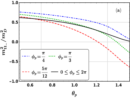
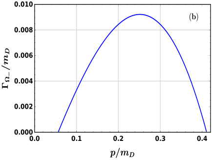
Figure 3: In the left panel, the squared value of the mass scale corresponding to $\Omega_{-}$ is plotted as a function of $\theta_{p}$ for three different values of $\phi_{p}=\{\pi/4,\pi/3,5\pi/12\}$ (shown in discrete style) considering $(\xi_{a},\xi_{b})=(-0.5,-0.9)$. The spheroidal case (shown in solid style) with $(\xi_{a},\xi_{b})=(0,-0.9)$ is also plotted for comparison. In the right panel, the growth rate for the $\Omega_{-}$ mode is plotted as a function of $p/m_{D}$ with $(\xi_{a},\xi_{b})=(-0.5,-0.9)$ and $(\theta_{p},\phi_{p})=(5\pi/12,5\pi/12)$.

IV Summary

In this article, we have studied the gluon polarization in presence of ellipsoidal momentum-space anisotropy. The momentum distribution function in our case is parametrized with two anisotropy parameters $\xi_{a}$ and $\xi_{b}$, represented together as an anisotropy tuple $\xi=(\xi_{a},\xi_{b})$. This is a simple generalization of the spheroidal RS form that has been extensively used in the literature. The general structure of the gluon polarization tensor in presence of such ellipsoidal anisotropy has been formulated and subsequently, the gluon effective propagator is obtained. As shown earlier, from the pole of the effective propagator, the three collective modes can be obtained in terms of the form factors. The results obtained using our formulation are in agreement with the previous study incorporating ellipsoidal anisotropy Kasmaei:2018yrr . It should be mentioned here that it is not mandatory to consider the general structure of the polarization function to obtain the collective modes, as, those can also be obtained solving the characteristic equation directly (see for example Kasmaei:2018yrr ). However, one of the important advantages of considering the general structure is that, the collective modes, as in our case, can be expressed in terms of the form factors which do not depend on the choice of the frame of reference. As a consequence, it is possible to define mass scales by taking the static limits of the functions characterizing the collective modes ($\Omega_{0}$ and $\Omega_{\pm}$) in a similar fashion as done in case of spheroidal anisotropy. The importance of such definition lies in the fact that, the existence of instability can be inferred systematically by studying the angular variations of the mass scales. More specifically, for the given external angles, the negative value of the squared mass indicates that the corresponding mode is unstable. In our analysis with $\xi_{a}=-0.5$ and $\xi_{b}=-0.9$, we have observed that, unlike the spheroidal case, the mode corresponding to $\Omega_{-}$ becomes unstable. The appearance of such additional unstable mode in presence of ellipsoidal anisotropy may have important influences on the isotropization of the QGP medium produced in HIC experiments. As mentioned earlier, the formulation, as developed in this work, will be particularly useful in the studies concerning the heavy quark potential in presence of ellipsoidal anisotropy. The usual procedure to obtain the hard-thermal loop resummed perturbative part of the heavy quark potential is to consider the Fourier transform of the 00 component of the effective propagator [obtained in Eq.(28)] in the static limits. Consequently, the nontrivial angular dependence enters in the potential through the mass scales. It should be noted that, in this work, only the retarded part of the gluon self energy is considered. On the other hand, the imaginary part of the potential can be obtained from the Feynman effective propagator in the real time Keldysh formalism Nopoush:2017zbu . Due to the azimuthal angular dependence of the mass scales, a nontrivial modification in the real as well as in the imaginary parts of the heavy quark potential is expected in presence of ellipsoidal anisotropy, which will be an interesting future direction.

V ACKNOWLEDGMENTS

R. G. is funded by University Grants Commission (UGC). B. K. is funded by Department of Atomic Energy (DAE), India via the project TPAES. A. M. acknowledges Najmul Haque for immense encouragement and support. A. M. would like to acknowledge Science and Engineering Research Board (SERB) for funding.

References

- (1) H. T. Ding, F. Karsch and S. Mukherjee, Int. J. Mod. Phys. E 24, no.10, 1530007 (2015) doi:10.1142/S0218301315300076 [arXiv:1504.05274 [hep-lat]].
- (2) C. Ratti, Rept. Prog. Phys. 81, no.8, 084301 (2018) doi:10.1088/1361-6633/aabb97 [arXiv:1804.07810 [hep-lat]].
- (3) A. Bazavov et al. [USQCD], Eur. Phys. J. A 55, no.11, 194 (2019) doi:10.1140/epja/i2019-12922-0 [arXiv:1904.09951 [hep-lat]].
- (4) E. Braaten and R. D. Pisarski, Nucl. Phys. B 337, 569-634 (1990) doi:10.1016/0550-3213(90)90508-B
- (5) J. O. Andersen and M. Strickland, Annals Phys. 317, 281-353 (2005) doi:10.1016/j.aop.2004.09.017 [arXiv:hep-ph/0404164 [hep-ph]].
- (6) N. Haque, A. Bandyopadhyay, J. O. Andersen, M. G. Mustafa, M. Strickland and N. Su, JHEP 05, 027 (2014) doi:10.1007/JHEP05(2014)027 [arXiv:1402.6907 [hep-ph]].
- (7) N. Su, Int. J. Mod. Phys. A 30, 1530025 (2015) doi:10.1142/S0217751X15300252 [arXiv:1502.04589 [hep-ph]].
- (8) C. Gale, S. Jeon and B. Schenke, Int. J. Mod. Phys. A 28, 1340011 (2013) doi:10.1142/S0217751X13400113 [arXiv:1301.5893 [nucl-th]].
- (9) S. Jeon and U. Heinz, Int. J. Mod. Phys. E 24, no.10, 1530010 (2015) doi:10.1142/S0218301315300106 [arXiv:1503.03931 [hep-ph]].
- (10) A. Jaiswal and V. Roy, Adv. High Energy Phys. 2016, 9623034 (2016) doi:10.1155/2016/9623034 [arXiv:1605.08694 [nucl-th]].
- (11) D. T. Son and A. O. Starinets, Ann. Rev. Nucl. Part. Sci. 57, 95-118 (2007) doi:10.1146/annurev.nucl.57.090506.123120 [arXiv:0704.0240 [hep-th]].
- (12) H. Nastase, [arXiv:0712.0689 [hep-th]].
- (13) R. Peschanski, Acta Phys. Polon. B 39, 2479-2510 (2008) [arXiv:0804.3210 [hep-ph]].
- (14) J. Sadeghi, B. Pourhassan and S. Heshmatian, Adv. High Energy Phys. 2013, 759804 (2013) doi:10.1155/2013/759804
- (15) Relativistic Heavy Ion Physics, R. Stock (Ed.), Springer, Heidelberg, 2010, ISBN: 978-3-642-01538-0 (Print) 978-3-642-01539-7 (Online)” doi:10.1007/978-3-642-01539-7.
- (16) W. Busza, K. Rajagopal and W. van der Schee, Ann. Rev. Nucl. Part. Sci. 68, 339-376 (2018) doi:10.1146/annurev-nucl-101917-020852 [arXiv:1802.04801 [hep-ph]].
- (17) M. Strickland, Pramana 84, no.5, 671-684 (2015) doi:10.1007/s12043-015-0972-1 [arXiv:1312.2285 [hep-ph]].
- (18) M. Strickland, Acta Phys. Polon. B 45, no.12, 2355-2394 (2014) doi:10.5506/APhysPolB.45.2355 [arXiv:1410.5786 [nucl-th]].
- (19) M. Alqahtani, M. Nopoush, R. Ryblewski and M. Strickland, Phys. Rev. Lett. 119, no.4, 042301 (2017) doi:10.1103/PhysRevLett.119.042301 [arXiv:1703.05808 [nucl-th]].
- (20) M. Alqahtani, M. Nopoush and M. Strickland, Prog. Part. Nucl. Phys. 101, 204-248 (2018) doi:10.1016/j.ppnp.2018.05.004 [arXiv:1712.03282 [nucl-th]].
- (21) S. Mrowczynski, A. Rebhan and M. Strickland, Phys. Rev. D 70, 025004 (2004) doi:10.1103/PhysRevD.70.025004 [arXiv:hep-ph/0403256 [hep-ph]].
- (22) S. Mrowczynski and M. H. Thoma, Phys. Rev. D 62, 036011 (2000) doi:10.1103/PhysRevD.62.036011 [arXiv:hep-ph/0001164 [hep-ph]].
- (23) P. Romatschke and M. Strickland, Phys. Rev. D 68, 036004 (2003) doi:10.1103/PhysRevD.68.036004 [arXiv:hep-ph/0304092 [hep-ph]].
- (24) P. Romatschke and M. Strickland, Phys. Rev. D 70, 116006 (2004) doi:10.1103/PhysRevD.70.116006 [arXiv:hep-ph/0406188 [hep-ph]].
- (25) B. Schenke and M. Strickland, Phys. Rev. D 74, 065004 (2006) doi:10.1103/PhysRevD.74.065004 [arXiv:hep-ph/0606160 [hep-ph]].
- (26) L. Bhattacharya, R. Ryblewski and M. Strickland, Phys. Rev. D 93, no.6, 065005 (2016) doi:10.1103/PhysRevD.93.065005 [arXiv:1507.06605 [hep-ph]].
- (27) L. Bhattacharya and P. Roy, Phys. Rev. C 78, 064904 (2008) doi:10.1103/PhysRevC.78.064904 [arXiv:0809.4596 [hep-ph]].
- (28) L. Bhattacharya and P. Roy, Phys. Rev. C 79, 054910 (2009) doi:10.1103/PhysRevC.79.054910 [arXiv:0812.1478 [hep-ph]].
- (29) M. Nopoush, Y. Guo and M. Strickland, JHEP 09, 063 (2017) doi:10.1007/JHEP09(2017)063 [arXiv:1706.08091 [hep-ph]].
- (30) B. Krouppa and M. Strickland, Universe 2, no.3, 16 (2016) doi:10.3390/universe2030016 [arXiv:1605.03561 [hep-ph]].
- (31) M. Mandal and P. Roy, Phys. Rev. D 86, 114002 (2012) doi:10.1103/PhysRevD.86.114002 [arXiv:1310.4657 [hep-ph]].
- (32) M. Mandal and P. Roy, Phys. Rev. D 88, no.7, 074013 (2013) doi:10.1103/PhysRevD.88.074013 [arXiv:1310.4660 [hep-ph]].
- (33) M. Mandal, L. Bhattacharya and P. Roy, Phys. Rev. C 84, 044910 (2011) doi:10.1103/PhysRevC.84.044910 [arXiv:1101.5855 [hep-ph]].
- (34) V. Chandra and V. Sreekanth, Eur. Phys. J. C 77, no.6, 427 (2017) doi:10.1140/epjc/s10052-017-4992-5 [arXiv:1602.07142 [nucl-th]].
- (35) M. Strickland, Braz. J. Phys. 37, 762-765 (2007) doi:10.1590/S0103-97332007000500021 [arXiv:hep-ph/0611349 [hep-ph]].
- (36) A. Rebhan, P. Romatschke and M. Strickland, Phys. Rev. Lett. 94, 102303 (2005) doi:10.1103/PhysRevLett.94.102303 [arXiv:hep-ph/0412016 [hep-ph]].
- (37) S. Mrowczynski, B. Schenke and M. Strickland, Phys. Rept. 682, 1-97 (2017) doi:10.1016/j.physrep.2017.03.003 [arXiv:1603.08946 [hep-ph]].
- (38) D. Bazow, U. W. Heinz and M. Strickland, Phys. Rev. C 90, no.5, 054910 (2014) doi:10.1103/PhysRevC.90.054910 [arXiv:1311.6720 [nucl-th]].
- (39) L. Tinti and W. Florkowski, Phys. Rev. C 89, no.3, 034907 (2014) doi:10.1103/PhysRevC.89.034907 [arXiv:1312.6614 [nucl-th]].
- (40) M. Nopoush, R. Ryblewski and M. Strickland, Phys. Rev. C 90, no.1, 014908 (2014) doi:10.1103/PhysRevC.90.014908 [arXiv:1405.1355 [hep-ph]].
- (41) M. Alqahtani, M. Nopoush and M. Strickland, Phys. Rev. C 92, no.5, 054910 (2015) doi:10.1103/PhysRevC.92.054910 [arXiv:1509.02913 [hep-ph]].
- (42) M. Nopoush and M. Strickland, Phys. Rev. C 100, no.1, 014904 (2019) doi:10.1103/PhysRevC.100.014904 [arXiv:1902.03303 [nucl-th]].
- (43) B. S. Kasmaei, M. Nopoush and M. Strickland, Phys. Rev. D 94, no.12, 125001 (2016) doi:10.1103/PhysRevD.94.125001 [arXiv:1608.06018 [hep-ph]].
- (44) B. S. Kasmaei and M. Strickland, Phys. Rev. D 102, no.1, 014037 (2020) doi:10.1103/PhysRevD.102.014037 [arXiv:1911.03370 [hep-ph]].
- (45) B. S. Kasmaei and M. Strickland, Phys. Rev. D 99, no.3, 034015 (2019) doi:10.1103/PhysRevD.99.034015 [arXiv:1811.07486 [hep-ph]].
- (46) B. S. Kasmaei and M. Strickland, Phys. Rev. D 97, no.5, 054022 (2018) doi:10.1103/PhysRevD.97.054022 [arXiv:1801.00863 [hep-ph]].
- (47) A. Dumitru, Y. Guo and M. Strickland, Phys. Lett. B 662, 37-42 (2008) doi:10.1016/j.physletb.2008.02.048 [arXiv:0711.4722 [hep-ph]].
- (48) A. Dumitru, Y. Guo and M. Strickland, Phys. Rev. D 79, 114003 (2009) doi:10.1103/PhysRevD.79.114003 [arXiv:0903.4703 [hep-ph]].
- (49) M. L. Bellac, “Thermal Field Theory,” doi:10.1017/CBO9780511721700