Randomized Quaternion Singular Value Decomposition for Low-Rank Approximation

Abstract

This paper presents a randomized quaternion singular value decomposition (QSVD) algorithm for low-rank matrix approximation problems, which are widely used in color face recognition, video compression, and signal processing problems. With quaternion normal distribution based random sampling, the randomized QSVD algorithm projects a high-dimensional data to a low-dimensional subspace and then identifies an approximate range subspace of the quaternion matrix. The key statistical properties of quaternion Wishart distribution are proposed and used to perform the approximation error analysis of the algorithm. Theoretical results show that the randomized QSVD algorithm can trace dominant singular value decomposition triplets of a quaternion matrix with acceptable accuracy. Numerical experiments also indicate the rationality of proposed theories. Applied to color face recognition problems, the randomized QSVD algorithm obtains higher recognition accuracies and behaves more efficient than the known Lanczos-based partial QSVD and a quaternion version of fast frequent directions algorithm.

1 Introduction

Low-rank approximations of quaternion matrices play an important role in color image processing area jns19nla ; jnw19 , in which color images are represented by pure quaternion matrices. Based on the color principal component analysis zjccg21 , the optimal rank-$k$ approximations preserve the main features and the important low frequency information of original color image samples. The core work of generating low-rank approximations is to compute the dominant quaternion singular value decomposition (QSVD) triplets (i.e., left singular vectors, singular values and right singular vectors). However, there are still few efficient algorithms to do this work when quaternion matrices are of large-scale sizes. No rigorous error analysis of computed approximations have also been given in the literature. In this paper, we present a new randomized QSVD algorithm and propose important theoretical results about the feasibility and the reliability of the algorithm.

In these years, quaternions ha and quaternion matrices zh have been more and more attractive in many research fields such as signal processing ebs14 , image data analysis bs ; jing21 , and machine learning minm17 ; zjccg21 . Because of non-commutative multiplication of quaternions, quaternion matrix computations contain more abundant challenging topics than real or complex matrix computations. The algorithms designed for quaternion matrices are also feasible for the real or complex case, but the converse is not always true. As we are concerned on, QSVD triplets can be achieved in three totally different ways. The first one is to call the svd command from Quaternion toolbox for Matlab (QTFM) developed by Sangwine and Bihan in 2005. For the principle of the algorithm, we refer to bs2 . The codes in QTFM are based on quaternion arithmetic operations and is less efficient for large matrices. The second one is to use the real structure-preserving QSVD method wl . Its main idea is to perform real operations on the real counterparts of quaternion matrices with structure preserving scheme. In practical implementations, only the first block row or column of the real counterpart is explicitly stored and updated, and the other subblocks are implicitly formulated with the aid of the algebraic symmetry structure. The real matrix-matrix multiplication-based BLAS-3 operations make the computation more efficient. The concept of structure-preserving was firstly proposed to solve quaternion eigenvalue problem in jwl , and then extended to the computations of quaternion LU lwz3 ; wm1 and QR lwz2 factorizations. Recently, Jia et al. jwzc developed a new structure-preserving quaternion QR algorithm for eigenvalue problems of general quaternion matrices, by constructing feasible frameworks of calculation for new quaternion Householder reflections and generalized Givens transformations. For more issues about structure-preserving algorithms, we refer to two monographs wl by Wei et al. and jia2019 by Jia. The above two ways are based on the truncation of the full QSVD and the computational cost is expensive in computing all singular values and corresponding left and right singular vectors. Thus they are not feasible for large-scale quaternion matrices. Jia et al. jns proposed a promising iterative algorithm to compute dominant QSVD triplets, based on the Lanczos bidiagonalization gv2 with reorthogonalization and thick-restart techniques. This method is referred to as the lansvdQ method. The superiority of lansvdQ method over the full QSVD was revealed in jns , through a number of practical applications such as color face recognition, video compression and color image completion. When the target rank $k$ increases, the matrix-vector products at each iteration of lansvdQ make the computational cost increase. Is there any method with lower computational cost for the quaternion low-rank approximation problem?

In the past decade, randomized algorithms for computing approximations of real matrices have been receiving more and more attention. Randomized projection and randomized sampling are two commonly used techniques to deal with large-scale problems efficiently. Randomized projection combines rows or columns together to produce a small sketch of $M\in{\mathbb{R}}^{m\times n}(m\geq n)$ sa2 . Possible techniques include subspace iterations gu , subspace embedding (SpEmb) mm , frequent directions (FD)glp and etc. Recently, Teng and Chu tc implanted SpEmb in FD to develop a fast frequent direction (SpFD) algorithm. Through the experimental results on world datasets and applications in network analysis, the superiority of SpFD over FD is displayed, not only in the efficiency, but also in the effectiveness.

Randomized sampling finds a small subset of rows or columns based on a pre-assigned probability distribution, say, by pre-multiplying $M$ on an $n\times\ell\leavevmode\nobreak\ (\ell\ll n)$ random Gaussian matrix $\Omega$, and identifies a low-dimensional approximate range subspace of $M$, after which a small-size matrix approximation is also obtained. The idea of a randomized sampling procedure can be traced to a 2006 technical report of paper mrt , and later analyzed and elaborated in dg ; gu ; hmt ; ma ; sa ; tc ; ygl ; zw . They are computationally efficient for large-scale problems and adapt to the case that the numerical rank is known or can be estimated in advance. When the singular values have relatively fast decay rate, the algorithm is inherently stable. For singular values with slow decay rate, the randomized algorithm with power scheme will enhance the stability of the algorithm.

In this paper we consider the randomized sampling algorithm for quaternion low-rank matrix approximations. The targeted randomized QSVD algorithm is expected to have lower computational cost and to be appropriate for choosing a small number of dominant QSVD triplets of large-scale quaternion matrices. It seems natural to utilize the research framework in hmt and generalize the real randomized SVD algorithm to quaternion matrices. Unfortunately, the theoretical analysis is long and arduous. It involves doses of statistics related to quaternion variables and several difficulties block us to go further.

• What kind of quaternion distribution is appropriate for the randomized QSVD algorithm? The proper quaternion distribution should be invariant under unitary transformations, which will bring convenience for approximation error analysis of the proposed algorithm. However, few studies have been seen on the probability distribution of quaternion variables in the literature.

• What are the distributions of the norms of the pseudoinverse ${\bf\Omega}^{\dagger}$ of quaternion random Gaussian matrix ${\bf\Omega}$? Due to the non-commutative multiplication of quaternions, quaternion determinant and integrals could not be defined similar to the real case. Hence, real probability theories could not be directly used to evaluate the norms of quaternion random Gaussian matrices.

• What are statistical evaluations of spectral norms of ${\bf\Omega}$ and its real counterpart? The real counter part $\Upsilon_{{\bf\Omega}}$ (see (2.1)) is a non-Gaussian random matrix. It is necessary to develop novel techniques to evaluate the expectation and probability bounds of $\|{\bf\Omega}\|_{2}$ and its scaled norms.

Based on the investigations on key features of ${\bf\Omega}$, we will give expectation and deviation bounds for approximation errors of the quaternion randomized SVD algorithm. To the best of our knowledge, these results are new and no developments have been made on the proposed algorithm and theories about quaternion matrix approximation problems. With high probability, the theoretical results show that the low rank approximations can be computed quickly for quaternion matrices with rapidly decaying singular values. Through the numerical experiments, the superiority of the proposed algorithm will be displayed, in comparison with the quaternion Lanczos method and a quaternion version of SpFD tc .

The paper is organized as follows. In Section 2, we review some preliminary results about quaternion matrices and randomized SVD for real matrices. The randomized QSVD algorithm and implement details for low-rank approximation problems will be studied in Section 3. In Section 4, the theoretical analysis is provided for the approximation errors. In Section 5, we test the theories and numerical behaviors of the proposed algorithms through several experiments and show their efficiency over Lanczos-based partial QSVD algorithm and quaternion SpFD for color face recognition problems.

Throughout this paper, we denote by ${\mathbb{R}}^{m\times n}$ and ${\mathbb{Q}}^{m\times n}$ the spaces of all $m\times n$ real and quaternion matrices, respectively. The norm $\|\cdot\|_{a}$ denotes either the spectral norm or the Frobenius norm. For quaternion matrix ${\bf A}\in{\mathbb{Q}}^{m\times n}$, ${\bf A}^{\dagger}$ is the pseudoinverse of ${\bf A}$, and ${\cal R}({\bf A})$ represents the column range space of ${\bf A}$. tr($\cdot$) denotes the trace of a quaternion or real square matrix, and etr($\cdot$)=exp(tr($\cdot$)) means the exponential operation of the trace. Let ${\sf P}\{\cdot\}$ denote the probability of an event and ${\sf E}(\cdot)$ denote the expectation of a random variable. For differentials ${\rm d}y_{1},{\rm d}y_{2}$ of real random variables $y_{1},y_{2}$, ${\rm d}y_{1}\wedge{\rm d}y_{2}$ denotes the non-commutative exterior product of ${\rm d}y_{1},{\rm d}y_{2}$, under which ${\rm d}y_{1}\wedge{\rm d}y_{2}=-{\rm d}y_{2}\wedge{\rm d}y_{1}$ and ${\rm d}y_{1}\wedge{\rm d}y_{1}=0$.

2 Preliminaries

In this section, we first introduce some basic information of quaternion matrices and quaternion SVD. The basic randomized SVD for real matrices is described thereafter.

2.1 Quaternion matrix and QSVD

The quaternion skew-field ${\mathbb{Q}}$ is an associative but non-commutative algebra of rank four over ${\mathbb{R}}$, and any quaternion ${\bf q}\in{\mathbb{Q}}$ has one real part and three imaginary parts given by ${\bf q}=q_{0}+q_{1}{\bf i}+q_{2}{\bf j}+q_{3}{\bf k},$ where $q_{0},q_{1},q_{2},q_{3}\in{\mathbb{R}}$, and i, j and k are three imaginary units satisfying ${\bf i}^{2}={\bf j}^{2}={\bf k}^{2}={\bf i}{\bf j}{\bf k}=-1.$ The conjugate and modulus of ${\bf q}$ are defined by ${\bf q}^{*}=q_{0}-q_{1}{\bf i}-q_{2}{\bf j}-q_{3}{\bf k}$ and $|{\bf q}|=\sqrt{q_{0}^{2}+q_{1}^{2}+q_{2}^{2}+q_{3}^{2}}$, respectively.

For any quaternion matrices ${\bf P}=P_{0}+P_{1}{\bf i}+P_{2}{\bf j}+P_{3}{\bf k}\in{\mathbb{Q}}^{m\times n}$, ${\bf Q}=Q_{0}+Q_{1}{\bf i}+Q_{2}{\bf j}+Q_{3}{\bf k}\in{\mathbb{Q}}^{m\times n}$, denote ${\bf Q}^{*}=Q_{0}^{T}-Q_{1}^{T}{\bf i}-Q_{2}^{T}{\bf j}-Q_{3}^{T}{\bf k}$ and the sum of ${\bf P},{\bf Q}$ as ${\bf P}+{\bf Q}=(P_{0}+Q_{0})+(P_{1}+Q_{1}){\bf i}+(P_{2}+Q_{2}){\bf j}+(P_{3}+Q_{3}){\bf k},$ and for quaternion matrix ${\bf S}\in{\mathbb{Q}}^{n\times\ell}$, the multiplication ${\bf QS}$ is given by

$$(Q_{0}S_{0}-Q_{1}S_{1}-Q_{2}S_{2}-Q_{3}S_{3})+(Q_{0}S_{1}+Q_{1}S_{0}+Q_{2}S_{3}-Q_{3}S_{2}){\bf i}+$$

$$(Q_{0}S_{2}-Q_{1}S_{3}+Q_{2}S_{0}+Q_{3}S_{1}){\bf j}+(Q_{0}S_{3}+Q_{1}S_{2}-Q_{2}S_{1}+Q_{3}S_{0}){\bf k}.$$

For ${\bf Q}\in{\mathbb{Q}}^{m\times n}$, define the real counterpart $\Upsilon_{\bf Q}$ and the column representation ${\bf Q}_{\rm c}$ as

$$\Upsilon_{\bf Q}=\left[\begin{array}[]{rrrr}Q_{0}&-Q_{1}&-Q_{2}&-Q_{3}\\ Q_{1}&Q_{0}&-Q_{3}&Q_{2}\\ Q_{2}&Q_{3}&Q_{0}&-Q_{1}\\ Q_{3}&-Q_{2}&Q_{1}&Q_{0}\end{array}\right],\qquad{\bf Q}_{\rm c}=\left[\begin{array}[]{c}Q_{0}\\ Q_{1}\\ Q_{2}\\ Q_{3}\end{array}\right].$$ (2.1)

Note that $\Upsilon_{\bf Q}$ has special real algebraic structure that is preserved under the following operationsjwl ; lwz2 :

$$\Upsilon_{k_{1}{\bf P}+k_{2}{\bf Q}}=k_{1}\Upsilon_{{\bf P}}+k_{2}\Upsilon_{{\bf Q}}\leavevmode\nobreak\ (k_{1},k_{2}\in{\mathbb{R}}),\leavevmode\nobreak\ \leavevmode\nobreak\ \Upsilon_{{\bf Q}^{*}}=\Upsilon_{{\bf Q}}^{T},\qquad\Upsilon_{{\bf QS}}=\Upsilon_{{\bf Q}}\Upsilon_{{\bf S}}.$$ (2.2)

For determinants of quaternion square matrices, a variety of definitions have emerged in terms of the complex and real counterparts to avoid the difficulties caused by the non-commutativity of quaternion multiplications; see lsm ; ro ; zh and reference therein. However these definitions do not coincide with the standard determinant of a real matrix. In this paper, we only consider the determinant of Hermitian quaternion matrices, which was defined by Li lsm as

$${\bf det}({\bf Q})=\lambda_{1}\lambda_{2}\cdots\lambda_{n},\quad{\bf Q}\in{\mathbb{Q}}^{n\times n}\mbox{ is Hermitian, }$$ (2.3)

where $\lambda_{1},\ldots,\lambda_{n}$ are eigenvalues of ${\bf Q}$, and they are proved to be real jwl ; lsm . This definition in (2.3) is consistent with the determinant of a real symmetric matrix, but does not adapt to the quaternion non-Hermitian matrices, since a quaternion non-Hermitian matrix has significantly different properties in its left and right eigenvalues, and there is no very close relation between left and right eigenvalues zh . When ${\bf Q}$ is Hermitian, the left and right eigenvalues are coincided to be the same real value. Throughout this paper we use ${\bf det}({\bf Q})$ to distinguish it from the real determinant symbol “det”. Moreover, if ${\bf Q}$ is positive semidefinite so that $\lambda_{i}\geq 0$, then the quaternion determinant ${\bf det}({\bf Q})$ can be represented in terms of a determinant of a real matrix lsm as

$${\bf det}({\bf Q})=\left[\det(\Upsilon_{\bf Q})\right]^{1/4},\quad{\bf Q}\mbox{ is Hermitian and positive semidefinite. }$$ (2.4)

Definition 1

The spectral norm (2-norm) of a quaternion vector ${\bf x}=[{\bf x}_{i}]\in{\mathbb{Q}}^{n}$ is $\|{\bf x}\|_{2}:=\sqrt{\sum_{i}|{\bf x}_{i}|^{2}}$. The 2-norm of a quaternion matrix ${\bf A}=[{\bf a}_{ij}]\in{\mathbb{Q}}^{m\times n}$ are $\|{\bf A}\|_{2}:=\max\sigma({\bf A})$, where $\sigma({\bf A})$ is the set of singular values of ${\bf A}$. The Frobenius norm of ${\bf A}$ is $\|{\bf A}\|_{F}=\big{(}\sum\limits_{i,j}|{\bf a}_{ij}|^{2}\big{)}^{1/2}=\left[{\rm tr}({\bf A}^{*}{\bf A})\right]^{1/2}.$

QSVD was firstly proposed in (zh, , Theorem 7.2) and the partial QSVD was presented in jns .

Lemma 1 (QSVD zh )

Let ${\bf A}\in{\mathbb{Q}}^{m\times n}$. Then there exist two quaternion unitary matrices ${\bf U}\in{\mathbb{Q}}^{m\times m}$ and ${\bf V}\in{\mathbb{Q}}^{n\times n}$ such that ${\bf U}^{*}{\bf AV}=\Sigma$, where $\Sigma={\rm diag}(\sigma_{1},\sigma_{2},\ldots,\sigma_{l})\in{\mathbb{R}}^{m\times n}$ with $\sigma_{i}\geq 0$ denoting the $i$-th largest singular value of ${\bf A}$ and $l=\min(m,n)$.

From jns , the optimal rank-$k$ approximation of ${\bf A}$ is given by ${\bf A}_{k}={\bf U}_{k}{\Sigma}_{k}{\bf V}_{k}^{*},$ where ${\bf U}_{k}$ and ${\bf V}_{k}$ are respectively submatrices of ${\bf U}$ and ${\bf V}$ by taking their first $k$ columns, and ${\Sigma}_{k}={\rm diag}(\sigma_{1},\ldots,\sigma_{k})$. Furthermore, by the real counterpart of QSVD: $\Upsilon_{\bf U}^{T}\Upsilon_{\bf A}\Upsilon_{\bf V}=\Upsilon_{\Sigma}$, where $\Upsilon_{\bf U}$ and $\Upsilon_{\bf V}$ are real orthogonal matrices, and $\Upsilon_{\Sigma}={\rm diag}(\Sigma,\Sigma,\Sigma,\Sigma)$. As a result, spectral and Frobenius norms of a quaternion matrix can be represented by the ones of real matrices as below

$$\|{\bf A}\|_{2}=\|\Upsilon_{\bf A}\|_{2},\qquad\|{\bf A}\|_{F}={1\over 2}\|\Upsilon_{\bf A}\|_{F}=\|{\bf A}_{\rm c}\|_{F}.$$ (2.5)

Moreover, for consistent quaternion matrices ${\bf A}$ and ${\bf B}$, it is obvious that

$$\|{\bf AB}\|_{F}\leq\|{\bf A}\|_{2}\|{\bf B}\|_{F},\quad\|{\bf AB}\|_{F}\leq\|{\bf A}\|_{F}\|{\bf B}\|_{2}.$$ (2.6)

2.2 Real randomized SVD and low-rank approximation

Given a real matrix $M\in\mathbb{R}^{m\times n}$, randomized sampling methods hmt ; lwm ; ma ; mrt ; wlr apply the input matrix $M$ onto a diverse set of random sample vectors $\Omega=[\omega_{1}\leavevmode\nobreak\ \ldots\leavevmode\nobreak\ \omega_{\ell}]$, expecting $M\Omega$ to capture the main information of the range space of $M$ and to maintain safe approximation error bounds with high probability. In hmt , a random Gaussian matrix $\Omega$ is used. By applying $M$ to $\Omega$, and then computing the orthogonormal basis $Q$ of the range space of $M\Omega$ via skinny QR factorization in Matlab:

$$\Omega=\texttt{randn}(n,\ell),\qquad[Q,\sim]=\texttt{ qr}(Y,0),\qquad\text{where}\leavevmode\nobreak\ Y=M\Omega,$$

one can get an approximate orthogonal range space of $M$. Here $\ell=k+p$ and $p$ is a small oversampling factor (say, $p=5$). In this case, the matrix $M$ is approximated by $M\approx QN,$ where $QQ^{T}$ is an orthogonal projector and the matrix $N:=Q^{T}M$ is of small size $\ell\times n$. The problem then reduces to compute the full SVD of $N$ as $N=\hat{U}\hat{S}\hat{V}^{T}$. Therefore $M\approx QN=Q\hat{U}\hat{S}\hat{V}^{T},$ and once a suitable rank $k$ has been chosen based on the decay of $\hat{S}$, the low-rank SVD factors can be determined as

$$\bar{U}_{k}=Q\hat{U}(:,1:k),\qquad\bar{S}_{k}=\hat{S}(1:k,1:k),\quad\mbox{and}\quad\bar{V}_{k}=\hat{V}(:,1:k)$$

such that $M_{k}\approx\bar{U}_{k}\bar{S}_{k}\bar{V}_{k}^{T}$. We refer to the above method as the randomized SVD.

The idea is simple, but whether the projection $QQ^{T}$ can capture the range of $M$ well depends not only on the property of random matrix, but also on the singular values $s_{i}$ of the matrix $M$ we are dealing with. It was shown in (hmt, , Theorems 10.5 and 10.6) that for $p\geq 2$, the expectation of the approximation error satisfies

$$\begin{array}[]{l}{\sf E}\|(I-QQ^{T})M\|_{2}\leq\Big{(}1+\sqrt{k\over p-1}\Big{)}s_{k+1}+{{\rm e}\sqrt{k+p}\over p}\Big{(}\sum\limits_{j=k+1}^{\min(m,n)}s_{j}^{2}\Big{)}^{1/2},\\ {\sf E}\|(I-QQ^{T})M\|_{F}\leq\Big{(}1+{k\over p-1}\Big{)}^{1/2}\Big{(}\sum\limits_{j=k+1}^{\min(m,n)}s_{j}^{2}\Big{)}^{1/2}.\end{array}$$ (2.7)

It is observed that when the singular values of $M$ decay very slowly, the method fails to work well, because the singular vectors associated with the tail singular values capture a significant fraction of the range of $M$, and the range of $Y=M\Omega$ as well. Power scheme can be used to enhance the effect of the approximation, i.e., by applying power operation to generate $Y=(MM^{T})^{q}M\Omega$, where $(MM^{T})^{q}M$ has the same singular space as $M$, but with a faster decay rate in its singular values.

3 Quaternion randomized SVD

In this section, we develop the randomized QSVD (randsvdQ) algorithm in Algorithm 1 and present some measures to improve the efficiency of the algorithm in practical implementations.

How to choose the random test matrix in the algorithm? Consider a simple case about the rank-1 approximation ${\bf A}_{1}=\sigma_{1}{\bf u}_{1}{\bf v}_{1}^{*}$ of the quaternion matrix ${\bf A}$. It is easy to prove that $\{{\bf y}_{*},{\bf z}_{*}\}=\{{\bf u}_{1},{\bf v}_{1}\}$ is the maximizer of $\max\limits_{\|{\bf y}\|_{2}=\|{\bf z}\|_{2}=1}|{\bf y}^{*}{\bf Az}|$, and $|{\bf y}^{*}\tilde{\bf z}|=|{\bf y}^{*}{\bf Az}|$ approximates $\sigma_{1}$ for ${\bf y}={\bf u}_{1}$ and $\tilde{\bf z}={\bf Av}_{1}\in{\cal R}({\bf A})$, in which the columns of ${\bf A}$ are spanned with quaternion coefficients. In order to capture the main information of ${\cal R}({\bf A})$ spanned by dominant left singular vectors of ${\bf A}$, it is natural to use a set of $n\times 1$ quaternion random vectors ${\bf\Omega}=[\bm{\omega}^{(1)}\leavevmode\nobreak\ \ldots\leavevmode\nobreak\ \bm{\omega}^{(\ell)}]$ to span the columns of ${\bf A}$, with random standard real Gaussian matrices as the four parts of ${\bf\Omega}$. That means the $n\times\ell$ quaternion random test matrix

$${\bf\Omega}={\Omega}_{0}+{\Omega}_{1}{\bf i}+{\Omega}_{2}{\bf j}+{\Omega}_{3}{\bf k},$$ (3.1)

where the entries of ${\Omega}_{0},{\Omega}_{1},{\Omega}_{2},{\Omega}_{3}$ are random and independently drawn from the $N(0,1)$-normal distribution. The detailed description of randomized QSVD is given in Algorithm 1.

Algorithm 1 ((randsvdQ) Randomized QSVD with fixed rank)

(1) Given ${\bf A}\in{\mathbb{Q}}^{m\times n}$, choose target rank $k$, oversampling parameter $p$ and the power scheme parameter $q$. Set $\ell=k+p$, and draw an $n\times\ell$ quaternion random test matrix ${\bf\Omega}$ as in (3.1).

(2) Construct ${\bf Y}_{0}={\bf A}{\bf\Omega}$ and for $i=1,2,\ldots,q$, compute

$$\hat{\bf Y}_{i}={\bf A}^{*}{\bf Y}_{i-1}\quad\mbox{ and }\quad{\bf Y}_{i}={\bf A}\hat{\bf Y}_{i}.$$

(3) Construct an ${m\times\ell}$ quaternion orthonormal basis ${\bf Q}$ for the range of ${\bf Y}_{q}$ by the quaternion QR decomposition and generate ${\bf B}={\bf Q}^{*}{\bf A}$.

(4) Compute the QSVD of a small-size matrix ${\bf B}$: ${\bf B}={{\bf\tilde{U}}}{{\tilde{\Sigma}}}{{\bf\tilde{V}}}^{*}$.

(5) Form the rank-$k$ approximation of ${\bf A}$: $\widehat{\bf A}_{k}^{(q)}={\hat{\bf U}}_{k}{\hat{\Sigma}}_{k}\hat{\bf V}_{k}^{*}$, where

$${\hat{\bf U}}_{k}={\bf Q}{\bf\tilde{U}}(:,1:k),\qquad{\hat{\Sigma}}_{k}={\tilde{\Sigma}}(1:k,1:k),\qquad\hat{\bf V}_{k}={\tilde{\bf V}}(:,1:k).$$

To implement Algorithm 1 efficiently, we recommend fast structure-preserving quaternion Householder QR jwzc ; lwz2 and QSVD algorithms wl ; lwz2 . Based on structure-preserving properties (2.2) of the real counterpart of a quaternion matrix, the essence of fast structure-preserving algorithm is to store the four parts $Q_{0},Q_{1},Q_{2},Q_{3}$ of a quaternion matrix ${\bf Q}$ only. When the left (or right) quaternion matrix transformation ${\bf T}_{l}$ (or ${\bf T}_{r}$) is applied on ${\bf Q}$, it is equivalent to implementing the real matrix multiplication $\Upsilon_{{\bf T}_{l}}{\Upsilon_{\bf Q}}$ (or ${\Upsilon_{\bf Q}}\Upsilon_{{\bf T}_{r}}$). In order to reduce the computational cost, only the first block column (or row) of ${\Upsilon_{\bf Q}}$ is updated and stored. Other blocks in the updated matrix are not explicitly stored and formed, and they can be determined according to the real symmetry structure. For example, in Step 2 of Algorithm 1, the four parts of quaternion matrices ${\bf Y}_{0}$, $\hat{\bf Y}_{i}$ and ${\bf Y}_{i}$ can be found from the computations of matrices

$$({\bf Y}_{0})_{\rm c}=\Upsilon_{\bf A}{\bf\Omega}_{\rm c},\quad\big{(}\hat{\bf Y}_{i}\big{)}_{\rm c}=\Upsilon_{\bf A}^{T}({\bf Y}_{i-1})_{\rm c},\quad\big{(}{\bf Y}_{i}\big{)}_{\rm c}=\Upsilon_{\bf A}\big{(}\hat{\bf Y}_{i}\big{)}_{\rm c},$$

respectively, and in Step 3, the four parts of quaternion matrix ${\bf B}$ can be found from ${\bf B}_{\rm c}=\Upsilon_{\bf Q}^{T}{\bf A}_{\rm c}$. Note that the computations of $({\bf Y}_{0})_{\rm c}:=\Upsilon_{\bf A}{\bf\Omega}_{\rm c}$ and the quaternion matrix multiplication ${\bf Y}_{0}={\bf A}{\bf\Omega}$ have the same real flops, while the former utilizes BLAS-3 based matrix-matrix operations better, and hence leads to efficient computations.

Once ${\bf Y}_{q}$ is obtained, the fast structure-preserving quaternion Householder QR algorithm lwz2 can be applied to get the orthonormal basis matrix ${\bf Q}$. Here the quaternion Householder transformation ${\bf H}$ to reduce a vector ${\bf u}\in{\mathbb{Q}}^{s}$ into ${\bf Hu}={\bf a}e_{1}$ in the QR process takes the form

$${\bf H}=I_{s}-2{\bf vv}^{*},\quad\mbox{with}\quad{\bf v}={{\bf u}-{\bf a}e_{1}\over\|{\bf u}-{\bf a}e_{1}\|_{2}},\quad{\bf a}=\left\{\begin{array}[]{ll}-{{\bf u}_{1}\over|{\bf u}_{1}|}\|{\bf u}\|_{2},&{\bf u}_{1}\not=0,\\ -\|{\bf u}\|_{2},&\mbox{otherwise},\end{array}\right.$$

where ${e}_{1}$ is the first column of the identity matrix $I_{s}$.

After computing ${\bf B}={\bf Q}^{*}{\bf A}$ in Step 3, the structure-preserving QSVD wl of ${\bf B}$ first factorizes ${\bf B}$ into a real bidiagonal matrix $\tilde{B}$ lwz2 , with the help of Golub and Reinsch’s idea gr and quaternion Householder transformation ${\bf H}_{0}$ lwz2 :

$${\bf H}_{0}{\bf u}:={\rm diag}\left({{\bf a}^{*}\over|{\bf a}|},I_{s-1}\right){\bf Hu}=|{\bf a}|e_{1}=\|{\bf u}\|_{2}e_{1}.$$ (3.2)

Afterwards, the standard SVD of the real matrix $\tilde{B}$ completes the QSVD algorithm.

Remark 1

The basis matrix ${\bf Q}$ in the algorithm is designed to approximate the left dominant singular subspace of ${\bf A}$. To get ${\bf Q}$, the structure-preserving quaternion Householder QR has better numerical stability through our numerous experiments, but with more computational cost since all columns of a unitary matrix are computed. Structure-preserving quaternion modified Gram-Schmidt (QMGS) (wl, , Chp. 2.4.3) is an economical alternative for getting the thin orthonormal factor ${\bf Q}$, but might lose the accuracy during the orthogonalization process when the input matrix has relatively small singular values. However, when we are dealing with low-rank approximation of a large input matrix, only a small number of dominant SVD triplets are taken into account, and QMGS sometimes is sufficient to get an orthonormal basis with expected accuracy (See Example 2 in Section 5).

Remark 2

If $\ell$ is much smaller than $n$, i.e., ${\bf B}$ is a “short-and-wide” matrix, the direct application of QSVD on ${\bf B}$ might lead to large computational cost. Alternatively, we recommend implementing the QMGS of ${\bf B}^{*}$ as

$${\bf B}^{*}=\hat{\bf Q}_{1}\hat{\bf R}_{1},\quad\mbox{ for}\qquad\hat{\bf Q}_{1}\in{\mathbb{Q}}^{n\times\ell},\qquad\hat{\bf R}_{1}\in{\mathbb{Q}}^{\ell\times\ell},$$ (3.3)

and then computing the QSVD of the $\ell\times\ell$ quaternion matrix $\hat{\bf R}_{1}$ as ${\hat{\bf R}}_{1}={\hat{\bf T}}_{1}{\hat{S}}_{1}{\hat{\bf Z}}_{1}^{*}$, from which the QSVD of ${\bf B}$ is given by ${\bf B}={{\bf\tilde{U}}}{{\tilde{\Sigma}}}{{\bf\tilde{V}}}^{*}$ for ${\bf\tilde{U}}={\hat{\bf Z}}_{1},{\tilde{\Sigma}}={\hat{S}}_{1}$ and ${\bf\tilde{V}}={\hat{\bf Q}_{1}}\hat{{\bf T}}_{1}$. We call the corresponding method the preconditioned randomized QSVD (prandsvdQ).

Remark 3

If ${\bf A}$ is Hermitian, it can be approximated as (hmt, , (5.13)):

$${\bf A}\approx{\bf Q}{\bf Q}^{*}{\bf AQ}{\bf Q}^{*}.$$ (3.4)

Then we form the matrix ${\bf B}={\bf Q}^{*}{\bf AQ}$, and use the structure-preserving eigQ algorithm in jwl to compute the eigen-decomposition of ${\bf B}$. The corresponding algorithm is referred to as the randeigQ algorithm in the context.

Note that both randeigQ and prandsvdQ reduce a large $n\times n$ problem into a smaller $\ell\times\ell$ problem. The essence of randeigQ computes the eigen-decomposition of a Hermitian matrix ${\bf Q}^{*}{\bf A\bf Q}$, while the prandsvdQ algorithm of ${\bf A}$ computes the QSVD of $\hat{\bf R}_{1}=\hat{\bf Q}_{1}^{*}{\bf AQ}$. For large problems with $\ell\ll n$, the cost of the two randomized algorithms is dominated by the quaternion QR procedure for getting ${\bf Q}$ and $\hat{\bf Q}_{1}$, and prandsvdQ will cost more CPU time for the extra computation of $\hat{\bf Q}_{1}$, but might be more accurate in estimating the eigenvalues of ${\bf A}$. That is because the columns of $\hat{\bf Q}_{1}$ span the range space ${\cal R}({\bf AQ})$, and it is exactly ${\cal R}({\bf A^{2}\Omega})$, while ${\bf Q}$ is the low-rank basis of ${\cal R}({\bf A}{\bf\Omega})$, therefore ${\cal R}({\bf\hat{Q}}_{1})$ might have a better approximation of the left dominant singular subspace than ${\cal R}({\bf Q})$. We will compare the numerical behaviors of the two algorithms in Section 5.

For the error approximation of randeigQ, if for some parameter $\varepsilon$, $\|(I_{m}-{\bf QQ}^{*}){\bf A}\|_{a}\leq\varepsilon$, then by (hmt, , (5.10)), the error of approximating ${\bf A}$ is given by $\|{\bf A}-{\bf QQ}^{*}{\bf A}{\bf QQ}^{*}\|_{a}\leq 2\varepsilon,$ where $\varepsilon$ will be evaluated in next section.

Remark 4

When the power scheme is not used in Algorithm 1 (i.e. $q=0$), note that the input matrix ${\bf A}$ in Algorithm 1 is revisited. However, in some circumstance, the matrix is too large to be stored. Using a similar technique to cw , we develop a method that requires just one pass over the matrix. For the input Hermitian matrix ${\bf A}$, according to (3.4) and ${\bf B}={\bf Q}^{*}{\bf AQ}$, the sample matrix

$${\bf Y}={\bf A\Omega}\approx{\bf Q}{\bf Q}^{*}{\bf AQ}{\bf Q}^{*}{\bf\Omega}={\bf Q}{\bf B}{\bf Q}^{*}{\bf\Omega},$$

and the approximation of the matrix ${\bf B}$ could be obtained by solving ${\bf BQ}^{*}{\bf\Omega}\approx{\bf Q}^{*}{\bf Y}.$

If ${\bf A}$ is not Hermitian, analogue to (hmt, , (5.14)-(5.15)), the single-pass algorithm can be constructed based on the relation ${\bf A}\approx{\bf Q}{\bf Q}^{*}{\bf A}{\bf\tilde{Q}}{\bf\tilde{Q}}^{*}$, where ${\bf\tilde{Q}}$ is the low-rank basis of ${\cal R}({\bf A}^{*})$ by applying ${\bf A}^{*}$ on a random test matrix ${\bf\tilde{\Omega}}$. The matrix ${\bf B}={\bf Q}^{*}{\bf A}{\bf\tilde{Q}}$ can be approximated by finding a minimum-residual solution to the system of relations ${\bf B\tilde{Q}^{*}\Omega}={\bf Q}^{*}{\bf Y}$, ${\bf B^{*}Q^{*}\tilde{\Omega}}={\bf\tilde{Q}}^{*}{\bf\tilde{Y}}$ for ${\bf Y}={\bf A\Omega}$ and ${\bf\tilde{Y}}={\bf A}^{*}{\bf\tilde{\Omega}}$.

4 Error analysis

The error analysis of Algorithm 3.1 consists of two parts, including the expected values of approximation errors $\|(I-{\bf QQ}^{*}){\bf A}\|_{a}=\|\widehat{\bf A}_{k+p}^{(q)}-{\bf A}\|_{a}$ in spectral or Frobenius norm, and the probability bounds of a large deviation as well. The argument relies on special statistical properties of quaternion test matrix ${\bf\Omega}$. Specially, we need to evaluate the Frobenius and spectral norms of ${\bf\Omega}$ and ${\bf\Omega}^{\dagger}$.

Our theories are established based on the framework of hmt . To start the analysis, we require to use the information of quaternion normal distributions, chi-squared and Wishart distributions. Some of results are provided in the literature, e.g. lo ; lsm , while some other information needs a rather lengthy deduction. In Section 4.1, we first summarize the main results in Theorems 4.1-4.3 to show the properties of quaternion randomized algorithm. After investigating the statistical properties of quaternion distributions in Section 4.2, we will give the detailed proofs of Theorems 4.1-4.3 in Section 4.3.

4.1 Main results

Theorem 4.1

(Average Frobenius error of the randsvdQ algorithm) Let the QSVD of the $m\times n$ ($m\geq n$) quaternion matrix ${\bf A}$ be

$${\bf A}={\bf U}\Sigma{\bf V}^{*}={\bf U}\left[\begin{array}[]{cc}\Sigma_{1}&0\\ 0&\Sigma_{2}\end{array}\right]\left[\begin{array}[]{c}{\bf V}_{1}^{*}\\ {\bf V}_{2}^{*}\end{array}\right],\quad\Sigma_{1}\in{\mathbb{R}}^{k\times k},\quad{\bf V}_{1}\in{\mathbb{Q}}^{n\times k},$$

where the singular value matrix $\Sigma={\rm diag}(\sigma_{1},\sigma_{2},\ldots,\sigma_{n})$ with $\sigma_{1}\geq\sigma_{2}\geq\cdots\geq\sigma_{n}\geq 0$, $k$ is the target rank. For oversampling parameter $p\geq 1$, let $q=0$, $\ell=k+p\leq n$ and the sample matrix ${\bf Y}_{0}={\bf A\Omega}$, where ${\bf\Omega}$ is an $n\times\ell$ quaternion random test matrix as in (3.1), and ${\bf\Omega}_{1}={\bf V}_{1}^{*}{\bf\Omega}$ is assumed to have full row rank, then the expected approximation error for the rank-($k+p$) matrix $\widehat{\bf A}_{k+p}^{(0)}$ via the power scheme-free randsvdQ algorithm satisfies

$${\sf E}\|\widehat{\bf A}_{k+p}^{(0)}-{\bf A}\|_{F}\leq\left(1+{\displaystyle 4k\over\displaystyle 4p+2}\right)^{1/2}\left(\sum\limits_{j>k}\sigma_{j}^{2}\right)^{1/2}.$$

Theorem 4.2

(Average spectral error of the randsvdQ algorithm) With the notations in Theorem 4.1, the expected spectral norm of the approximation error in the power scheme-free algorithm satisfies

$${\sf E}\|\widehat{\bf A}_{k+p}^{(0)}-{\bf A}\|_{2}\leq\left(1+3\sqrt{k\over 4p+2}\leavevmode\nobreak\ \right)\sigma_{k+1}+{3{\rm e}\sqrt{4k+4p+2}\over 2p+2}\Big{(}\sum\limits_{j>k}\sigma_{j}^{2}\Big{)}^{1/2}.$$ (4.1)

If $q>0$ and the power scheme is used, then for the rank-$(k+p)$ matrix $\widehat{\bf A}_{k+p}^{(q)}$, the spectral error satisfies

$${\sf E}\|\widehat{\bf A}_{k+p}^{(q)}-{\bf A}\|_{2}\leq\left[\left(1+3\sqrt{k\over 4p+2}\leavevmode\nobreak\ \right)\sigma_{k+1}^{2q+1}+{3{\rm e}\sqrt{4k+4p+2}\over 2p+2}\left(\sum\limits_{j>k}\sigma_{j}^{2(2q+1)}\right)^{1/2}\right]^{1/(2q+1)}.$$

Theorem 4.3

(Deviation bound for approximation errors of the randsvdQ algorithm) With the notations in Theorem 4.1, we have the following estimate for the Frobenius error

$$\|\widehat{\bf A}_{k+p}^{(0)}-{\bf A}\|_{F}\leq\Big{(}1+t\sqrt{3k\over p+1}\Big{)}\Big{(}\sum\limits_{j>k}\sigma_{j}^{2}\Big{)}^{1/2}+ut{{\rm e}\sqrt{4k+4p+2}\over 4p+4}\sigma_{k+1},$$ (4.2)

except with the probability $2t^{-4p}+{\rm e}^{-u^{2}/2}$. For the spectral error,

$$\|\widehat{\bf A}_{k+p}^{(0)}-{\bf A}\|_{2}\leq\left(1+{3t\over 2}\sqrt{3k\over p+1}+ut\eta_{k,p}\right)\sigma_{k+1}+3t\eta_{k,p}\left(\sum\limits_{j>k}\sigma_{j}^{2}\right)^{1/2},$$ (4.3)

except with the probability $2t^{-4p}+{\rm e}^{-u^{2}/2}$, in which $\eta_{k,p}={{\rm e}\sqrt{4k+4p+2}\over 4p+4}$.

Theorems 4.1-4.3 reveal that the performance of the randomized algorithm depends strongly on the properties of singular values of ${\bf A}$. When the singular values of ${\bf A}$ have fast decay rate, it is much easier to identify a good low-rank basis ${\bf Q}$ and provide acceptable error bounds. However, when the singular values of ${\bf A}$ decay slowly, the constructed basis ${\bf Q}$ may have low accuracy, and the power scheme will increase the decay rate of the singular values of ${\bf C}=({\bf AA^{*}})^{q}{\bf A}$, and generate a better low-rank basis matrix.

4.2 Statistical analysis of quaternion random test matrix

In this subsection, we aim to investigate Frobenius and spectral norms of the quaternion test matrix ${\bf G}$ and its pseudoinverse, where

$${\bf G}=G_{0}+G_{1}{\bf i}+G_{2}{\bf j}+G_{3}{\bf k}\in{\mathbb{Q}}^{m\times n},\quad m\leq n,$$ (4.4)

and $G_{0},\ldots,G_{3}$ are standard Gaussian matrices whose entries are random and independently drawn from the normal distribution $N(0,1)$. Note that the norms of $\|{\bf G}^{{\dagger}}\|_{a}$ for $a=2,F$ are closely related to the measure of $\big{(}{\bf G}{\bf G}^{*}\big{)}^{-1}$, where the matrix ${\bf G}{\bf G}^{*}$ is named as a quaternion Wishart matrix. As a result, we first recall some well known results about the quaternion normal distribution and Wishart distribution.

Definition 2 (tf )

Let ${\bf z}=z_{0}+z_{1}{\bf i}+z_{2}{\bf j}+z_{3}{\bf k}$ be a random $m\times 1$ quaternion vector with zero mean. Define the quaternion covariance matrix ${\bf\Sigma}_{m}={\bf cov}({\bf z},{\bf z})={\sf E}({\bf z}{\bf z}^{*})$ as

$${\bf\Sigma}_{m} = {\sf E}[(z_{0}+z_{1}{\bf i}+z_{2}{\bf j}+z_{3}{\bf k})(z_{0}^{T}-z_{1}^{T}{\bf i}-z_{2}^{T}{\bf j}-z_{3}^{T}{\bf k})]$$

$$= \Sigma_{00}+\Sigma_{11}+\Sigma_{22}+\Sigma_{33}+(-\Sigma_{01}+\Sigma_{10}-\Sigma_{23}+\Sigma_{32}){\bf i}$$

$$+(-\Sigma_{02}+\Sigma_{13}+\Sigma_{20}-\Sigma_{31}){\bf j}+(-\Sigma_{03}+\Sigma_{30}-\Sigma_{12}+\Sigma_{21}){\bf k},$$

in which $\Sigma_{ij}={\rm cov}(z_{i},z_{j})\in{\mathbb{R}}^{m\times m}$ is the real covariance of random vectors $z_{i}$ and $z_{j}$.

In particular, when the four parts $z_{0},z_{1},z_{2},z_{3}$ of the quaternion vector ${\bf z}$ are real independent random vectors drawn from the normal distribution $N(0,I_{m})$, then the quaternion random vector ${\bf z}$ follows the quaternion normal distribution ${\bf N}(0,4I_{m})$ law, with the possibility density function (pdf)tf : ${\sf pdf}({\bf z})=(2\pi)^{-2m}{\rm etr}(-{1\over 2}{\bf z^{*}z}).$ We remark that when ${\bf z}\sim{\bf N}(0,4I_{m})$, $\|{\bf z}\|_{2}^{2}$ represents the sum of $4m$ independent real variables and each variable follows $N(0,1)$ law. Thus by the concept of real chi-squared distribution, $\|{\bf z}\|_{2}^{2}$ follows real chi-squared distribution $\chi_{4m}^{2}$ with $4m$ degrees of freedom.

The following lemma indicates that the quaternion normal distribution ${\bf N}(0,4I_{m})$ is unitarily invariant.

Lemma 2 (lsm )

For an $m\times 1$ quaternion random vector ${\bf z}\sim{\bf N}(0,4I_{m})$, let ${\bf y}={\bf Bz}+{\bf u}$, where ${\bf B}$ is an $m$-by-$m$ nonsingular quaternion matrix, and ${\bf u}$ is an $m$-by-1 quaternion vector, then ${\bf y}\sim{\bf N}({\bf u},4{\bf BB}^{*})$.

The rigorous definition of the Wishart distribution is given as follows.

Definition 3 (tf ; tl )

Let ${\bf Z}=[{\bf z}_{1}\leavevmode\nobreak\ {\bf z}_{2}\leavevmode\nobreak\ \ldots\leavevmode\nobreak\ {\bf z}_{n}]$, where ${\bf z}_{1},\ldots,{\bf z}_{n}$ are $m\times 1$ random independent quaternion vectors drawn from the same distribution, i.e., ${\bf z}_{i}\sim{\bf N}(0,{\bf\Sigma})(1\leq i\leq n)$. Then ${\bf A}={\bf Z}{\bf Z}^{*}\in{\mathbb{Q}}^{m\times m}$ is said to have the quaternion Wishart distribution with $n$ degrees of freedom and covariance matrix ${\bf\Sigma}$. We will write that ${\bf A}\sim{\bf W}_{m}(n,{\bf\Sigma})$.

Note that the matrix ${\bf\Sigma}$ could be quaternion or real. In this paper, we are only interested in the real case and use the notation $\Sigma$ for a distinguishment. The matrix ${\bf A}$ is singular when $n<m$, and the pdf of ${\bf A}$ doesn’t exist in this case. When $m\leq n$, the pdf lsm ; tl (See also (lo, , Theorem 4.2.1)) of ${\bf A}$ exists. Before giving the pdf, we first recall the definitions of exterior products, which are vital for the volume element of a multivariate density function.

Definition 4 (mu ; lsm )

For any $m\times n$ real matrix $X$, let ${\rm d}X=[{\rm d}x_{ij}]$ denote the matrix of differentials, define the $mn$-exterior product $\{{\rm d}X\}$ of the $mn$ distinct and free elements in $X$ as $\{{\rm d}X\}\equiv\mathop{\wedge}\limits_{i,j}{\rm d}x_{ij}.$ For any $m\times n$ quaternion matrix ${\bf X}=X_{0}+{X_{1}}{\bf i}+{X_{2}}{\bf j}+{X_{3}}{\bf k}$, denote ${\rm d}{\bf X}={\rm d}X_{0}+{\rm d}X_{1}\leavevmode\nobreak\ {\bf i}+{\rm d}X_{2}\leavevmode\nobreak\ {\bf j}+{\rm d}X_{3}\leavevmode\nobreak\ {\bf k}$, and define $\{{\rm d}{\bf X}\}=\{{\rm d}{X}_{0}\}\wedge\{{\rm d}{X}_{1}\}\wedge\{{\rm d}{X}_{2}\}\wedge\{{\rm d}{X}_{3}\}$. If ${\bf X}$ is Hermitian, then $X_{0}$ is symmetric, while $X_{2},X_{3},X_{4}$ are skew-symmetric, and $\{{\rm d}{\bf X}\}$ takes the form

$$\{{\rm d}{\bf X}\}=\Big{(}\mathop{\wedge}\limits_{i\leq j}^{m}{\rm d}({X_{0}})_{ij}\Big{)}\wedge\Big{(}\mathop{\wedge}\limits_{i<j}^{m}{\rm d}({X_{1}})_{ij}\Big{)}\wedge\Big{(}\mathop{\wedge}\limits_{i<j}^{m}{\rm d}({X_{2}})_{ij}\Big{)}\wedge\Big{(}\mathop{\wedge}\limits_{i<j}^{m}{\rm d}({X_{3}})_{ij}\Big{)}.$$

In the definition, the exterior product of differential form in different order might differ by a factor $\pm 1$. Since we are integrating exterior differential forms representing probability density functions, we ignore the sign of exterior differential forms for the sake of convenience. Based on the notation for the exterior product, the pdf of the quaternion Wishart matrix is given as follows.

Lemma 3 (lsm ; lo )

Let the quaternion Wishart matrix ${\bf A}\sim{\bf W}_{m}(n,{\Sigma})$, then the pdf of ${\bf A}$ satisfies

$${\sf pdf}({\bf A})\{{\rm d}{\bf A}\}=\beta_{m,n}\left[{\rm det}({\Sigma})\right]^{-2n}\left[{\bf det}({\bf A})\right]^{2(n-m)+1}{\rm etr}(-2\Sigma^{-1}{\bf A})\{{\rm d}{\bf A}\},$$ (4.5)

in which $\{{\rm d}{\bf A}\}$ represents the volume element of this multivariate density function, and

$$\beta_{m,n}=2^{2mn}\pi^{-m(m-1)}\left(\prod\limits_{i=1}^{m}\Gamma\big{(}2(n-i+1)\big{)}\right)^{-1},$$

with the Gamma function $\Gamma(\cdot)$ defined by $\Gamma(x)={\displaystyle\int_{0}^{\infty}}t^{x-1}{\rm e}^{-t}dt(x>0)$.

The properties of the quaternion Wishart matrix are given as follows.

Theorem 4.4

Given ${\bf A}\sim{\bf W}_{m}(n,{\Sigma})$.

(i) For ${\bf M}\in{\mathbb{Q}}^{k\times m}$ with ${\rm rank}({\bf M})=k$, we have ${\bf MAM}^{*}\sim{\bf W}_{k}(n,{\bf M}{\Sigma}{\bf M}^{*}).$

(ii) Partition

$${\bf A}=\left[\begin{array}[]{cc}{\bf A}_{11}&{\bf A}_{12}\\ {\bf A}_{12}^{*}&{\bf A}_{22}\end{array}\right],\quad{\Sigma}=\left[\begin{array}[]{cc}{\Sigma}_{11}&{\Sigma}_{12}\\ {\Sigma}_{21}&{\Sigma}_{22}\end{array}\right],$$

in which ${\bf A}_{11}\in{\mathbb{Q}}^{k\times k}$, $\Sigma_{11}\in{\mathbb{R}}^{k\times k}$. Let ${\bf A}_{11,2}={\bf A}_{11}-{\bf A}_{12}{\bf A}_{22}^{-1}{\bf A}_{12}^{*}$, ${\Sigma}_{11,2}={\Sigma}_{11}-{\Sigma}_{12}{\Sigma}_{22}^{-1}{\Sigma}_{21}$, then

$${\bf A}_{11,2}\sim{\bf W}_{k}(n-m+k,{\Sigma}_{11,2}).\\$$

Proof

(i) Note that ${\bf A}=\sum\limits_{i=1}^{n}{\bf z}_{i}{\bf z}_{i}^{*}$ with ${\bf z}_{i}\sim{\bf N}(0,\Sigma)$. It follows that $\hat{\bf z}_{i}:=2\Sigma^{-1/2}{\bf z}_{i}\sim{\bf N}(0,4I_{m})$ from the definition of quaternion covariance. By applying Lemma 2, ${\bf Mz}_{i}={1\over 2}({\bf M}\Sigma^{1/2}\hat{\bf z}_{i})\sim{\bf N}(0,{\bf M}\Sigma{\bf M}^{*})$, and hence

$${\bf MAM}^{*}=\sum\limits_{i=1}^{n}{\bf Mz}_{i}({\bf Mz}_{i})^{*}\sim{\bf W}_{k}(n,{\bf M}\Sigma{\bf M}^{*}).$$

(ii) Let ${\bf Z}=\left[\begin{array}[]{cc}I_{k}&0\\ -{\bf A}_{22}^{-1}{\bf A}_{12}^{*}&I_{m-k}\end{array}\right]$, and change the variables of ${\bf A}$ into ${\bf A}_{11,2}$, ${\bf B}_{12}={\bf A}_{12}$ and ${\bf B}_{22}={\bf A}_{22}$ through the following transformation

$${\bf A}{\bf Z}:=\left[\begin{array}[]{cc}{\bf A}_{11}&{\bf A}_{12}\\ {\bf A}_{12}^{*}&{\bf A}_{22}\end{array}\right]\left[\begin{array}[]{cc}I_{k}&0\\ -{\bf A}_{22}^{-1}{\bf A}_{12}^{*}&I_{m-k}\end{array}\right]=\left[\begin{array}[]{cc}{\bf A}_{11,2}&{\bf B}_{12}\\ 0&{\bf B}_{22}\end{array}\right].$$ (4.6)

The quaternion matrix ${\bf Z}$ is not Hermitian, and ${\bf det}({\bf Z})$ is not well defined. In order to express ${\bf det}({\bf A})$ in terms of ${\bf det}({\bf A}_{11,2})$ and ${\bf det}({\bf B}_{22})$, we consider the transformation ${\bf Z}^{*}{\bf A}{\bf Z}$ to get ${\bf Z}^{*}{\bf A}{\bf Z}={\rm diag}({\bf A}_{11,2},{\bf B}_{22})=:{\bf F},$ where ${\bf A}_{11,2}$ and ${\bf B}_{22}$ are Hermitian and positive definite matrices.

Take the real counter parts on both sides of ${\bf Z}^{*}{\bf A}{\bf Z}={\bf F}$, the properties in (2.2) gives $\Upsilon_{\bf Z}^{T}\Upsilon_{\bf A}\Upsilon_{\bf Z}=\Upsilon_{\bf F}$ and the standard determinant of real matrix $\Upsilon_{\bf F}$ satisfies

$$\det(\Upsilon_{\bf F})=\left(\det(\Upsilon_{\bf Z})\right)^{2}\det(\Upsilon_{\bf A}),$$ (4.7)

where by writing the (2,1)-subblock of ${\bf Z}$ as $-{\bf A}_{22}^{-1}{\bf A}_{12}^{*}=\bar{A}_{0}+\bar{A}_{1}{\bf i}+\bar{A}_{2}{\bf j}+\bar{A}_{3}{\bf k}$, and using the identity matrices in block columns 2,4,6,8 of $\Upsilon_{\bf Z}$:

$$\Upsilon_{\bf Z}=\left[\begin{array}[]{cc|cc|cc|cc}I&0&0&0&0&0&0&0\\ \bar{A}_{0}&I&-\bar{A}_{1}&0&-\bar{A}_{2}&0&-\bar{A}_{3}&0\\ \hline\cr 0&0&I&0&0&0&0&0\\ \bar{A}_{1}&0&\bar{A}_{0}&I&-\bar{A}_{3}&0&\bar{A}_{2}&0\\ \hline\cr 0&0&0&0&I&0&0&0\\ \bar{A}_{2}&0&\bar{A}_{3}&0&\bar{A}_{0}&I&-\bar{A}_{1}&0\\ \hline\cr 0&0&0&0&0&0&I&0\\ \bar{A}_{3}&0&-\bar{A}_{2}&0&\bar{A}_{1}&0&\bar{A}_{0}&I\end{array}\right]$$

to eliminate the subblocks $\pm\bar{A}_{i}$ to zero, we get $\det(\Upsilon_{\bf Z})=\det(I_{4m})=1$. Thus in (4.7), $\det(\Upsilon_{\bf A})=\det(\Upsilon_{\bf F})$. The applications of (2.4) and the definition (2.3) to this equality give

$${\bf det}({\bf A})={\bf det}({\bf F})={\bf det}({\bf A}_{11,2}){\bf det}({\bf B}_{22}).$$ (4.8)

For the real matrix $\Sigma$, it is obvious that

$$\det(\Sigma)=\det({\Sigma}_{22})\det({\Sigma}_{11,2}).$$ (4.9)

By putting ${C}={\Sigma}^{-1}=\left[\begin{array}[]{cc}{C}_{11}&{C}_{12}\\ {C}_{21}&{C}_{22}\end{array}\right],$ we conclude that ${C}_{11}={\Sigma}_{11,2}^{-1}$ and

$$\begin{array}[]{rl}{\rm tr}({\Sigma}^{-1}{\bf A})&={\rm tr}\left(\left[\begin{array}[]{cc}{C}_{11}&{C}_{12}\\ {C}_{21}&{C}_{22}\end{array}\right]\left[\begin{array}[]{cc}{\bf A}_{11,2}+{\bf B}_{12}{\bf B}_{22}^{-1}{\bf B}_{12}^{*}&{\bf B}_{12}\\ {\bf B}_{12}^{*}&{\bf B}_{22}\end{array}\right]\right)\\ &={\rm tr}(C_{11}{\bf A}_{11,2})+{\rm tr}({\bf\Delta}_{1})+{\rm tr}({\bf\Delta}_{2})={\rm tr}({\Sigma}_{11,2}^{-1}{\bf A}_{11,2})+{\rm tr}({\bf\Delta}_{1})+{\rm tr}({\bf\Delta}_{2}),\end{array}$$ (4.10)

where ${\bf\Delta}_{1}={\Sigma}_{11,2}^{-1}{\bf B}_{12}{\bf B}_{22}^{-1}{\bf B}_{12}^{*}+{C}_{12}{\bf B}_{12}^{*},{\bf\Delta}_{2}={C}_{21}{\bf B}_{12}+{C}_{22}{\bf B}_{22}.$

Note that the differential of ${\bf A}_{12}{\bf A}_{22}^{-1}{\bf A}_{12}^{*}$ satisfies

$${\rm d}({\bf A}_{12}{\bf A}_{22}^{-1}{\bf A}_{12}^{*})=({\rm d}{\bf A}_{12}){\bf A}_{22}^{-1}{\bf A}_{12}^{*}+{\bf A}_{12}({\rm d}{\bf A}_{22}^{-1}){\bf A}_{12}^{*}+{\bf A}_{12}{\bf A}_{22}^{-1}({\rm d}{\bf A}_{12}^{*}),$$

in which the differential ${\rm d}({\bf A}_{22}^{-1})$ can be derived by differentiating ${\bf A}_{22}^{-1}{\bf A}_{22}=I_{m-k}$ as

$$({\rm d}{\bf A}_{22}^{-1}){\bf A}_{22}+{\bf A}_{22}^{-1}({\rm d}{\bf A}_{22})=0,\quad\mbox{or equivalently,}\quad{\rm d}{\bf A}_{22}^{-1}=-{\bf A}_{22}^{-1}({\rm d}{\bf A}_{22}){\bf A}_{22}^{-1}.$$

Since the exterior products of repeated differentials are zero, we then get $\{{\rm d}({\bf A}_{12}{\bf A}_{22}^{-1}{\bf A}_{12}^{*})\}\wedge\{{\rm d}{\bf A}_{12}\}\wedge\{{\rm d}{\bf A}_{22}\}=0.$ Thus

$$\begin{array}[]{rl}\{{\rm d}{\bf A}\}&=\{{\rm d}{\bf A}_{11}\}\wedge\{{\rm d}{\bf A}_{12}\}\wedge\{{\rm d}{\bf A}_{22}\}=\{{\rm d}({\bf A}_{11}-{\bf A}_{12}{\bf A}_{22}^{-1}{\bf A}_{12}^{*})\}\wedge\{{\rm d}{\bf A}_{12}\}\wedge\{{\rm d}{\bf A}_{22}\}\\ &=\{{\rm d}{\bf A}_{11,2}\}\wedge\{{\rm d}{\bf B}_{12}\}\wedge\{{\rm d}{\bf B}_{22}\}.\end{array}$$ (4.11)

Substituting (4.8)-(4.11) into ${\sf pdf}({\bf A})\{{\rm d}{\bf A}\}$ in Lemma 3, we obtain

$$\begin{array}[]{l}{\sf pdf}({\bf A})\{{\rm d}{\bf A}\}=\beta_{m,n}\left([\det({\Sigma}_{11,2})]^{-2n}\left[{\bf det}({\bf A}_{11,2})\right]^{2(n-m)+1}{\rm etr}(-2{\Sigma}_{11,2}^{-1}{\bf A}_{11,2})\right)\\ \quad\times\left([\det({\Sigma}_{22})]^{-2n}\left[{\bf det}({\bf B}_{22})\right]^{2(n-m)+1}{\rm etr}(-2{\bf\Delta}_{1}){\rm etr}(-2{\bf\Delta}_{2})\right)\{{\rm d}{\bf A}_{11,2}\}\wedge\{{\rm d}{\bf B}_{12}\}\wedge\{{\rm d}{\bf B}_{22}\},\end{array}$$ (4.12)

from which we see that ${\bf A}_{11,2}$ is independent of ${\bf B}_{12},{\bf B}_{22}$, because of the density function factors. Notice that ${\bf A_{11,2}}$ is $k\times k$, and $\left[{\bf det}({\bf A}_{11,2})\right]^{2(n-m)+1}=\left[{\bf det}({\bf A}_{11,2})\right]^{2((n-m+k)-k)+1}.$ Moreover, the terms in (4.12) including ${\bf A}_{11,2}$ have close relations to the pdf of a Wishart matrix, therefore we can find the ${\sf pdf}$ of ${\bf A_{11,2}}$ from ${\sf pdf}({\bf A})$ so that ${\sf pdf}({\bf A_{11,2}})$ takes the form

$$\begin{array}[]{l}\beta_{k,n-m+k}[{\rm det}({\Sigma}_{11,2})]^{-2(n-m+k)}\left[{\bf det}({\bf A}_{11,2})\right]^{2((n-m+k)-k)+1}{\rm etr}(-2{\Sigma}_{11,2}^{-1}{\bf A}_{11,2}),\end{array}$$

which means ${\bf A}_{11,2}\sim{\bf W}_{k}(n-m+k,{\Sigma}_{11,2})$. The remaining terms in (4.12) correspond to the joint pdf of ${\bf B}_{12}$, ${\bf B}_{22}$, whose distributions will not be considered here.

Theorem 4.4 includes the properties of a real Wishart matrix (mu, , Theorems 3.2.5 and 3.2.10) as special cases. With Theorem 4.4, the expectation of $\|{\bf G}^{\dagger}\|_{F}^{2}$ is deduced in the following theorem.

Theorem 4.5

Let the quaternion random matrix ${\bf G}\in{\mathbb{Q}}^{m\times n}$($m\leq n$) be given by (4.4). Then the expectation of $\|{\bf G}^{\dagger}\|_{F}^{2}$ satisfies

$${\sf E}\|{\bf G}^{\dagger}\|_{F}^{2}={\displaystyle m\over 4(n-m)+2}.$$

Proof

It is obvious that each column in ${\bf G}$ follows ${\bf N}(0,4I_{m})$ and

$${\sf E}\|{\bf G}^{\dagger}\|_{F}^{2}={\sf E}\left({\rm tr}\left[({\bf GG}^{*})^{-1}\right]\right)={\sf E}\sum\limits_{i=1}^{m}(e_{i}^{T}{\bf A}^{-1}e_{i})=\sum\limits_{i=1}^{m}{\sf E}(e_{i}^{T}{\bf A}^{-1}e_{i}),$$ (4.13)

where $e_{i}$ is the $i$-th column of the identity matrix $I_{m}$, and ${\bf A}={\bf G}{\bf G}^{*}\sim{\bf W}_{m}(n,4I_{m})$.

For each fixed $i$, let $\Pi_{1,i}$ be the permutation matrix obtained by interchanging columns $1,i$ in the $m\times m$ identity matrix, and denote ${\bf C}=\Pi_{1,i}^{T}{\bf A}\Pi_{1,i}=\left[\begin{array}[]{cc}{\bf C}_{11}&{\bf C}_{12}\\ {\bf C}_{21}&{\bf C}_{22}\end{array}\right]$ with ${\bf C}_{11}\in{\mathbb{Q}}^{1\times 1},$ then ${\bf C}\sim{\bf W}_{m}(n,4I_{m})$ by Theorem 4.4(i). Moreover, $\left(e_{i}^{T}{\bf A}^{-1}e_{i}\right)^{-1}=\left(e_{1}^{T}{\bf C}^{-1}e_{1}\right)^{-1}={\bf C}_{11}-{\bf C}_{12}{\bf C}_{22}^{-1}{\bf C}_{21}.$

According to Theorem 4.4(ii), $\left(e_{i}^{T}{\bf A}^{-1}e_{i}\right)^{-1}\sim{\bf W}_{1}(n-m+1,4),$ indicating that there exists an $(n-m+1)$-dimensional quaternion column vector ${\bf z}\sim{\bf N}(0,4I_{n-m+1})$ satisfying

$$\left(e_{i}^{T}{\bf A}^{-1}e_{i}\right)^{-1}=\|{\bf z}\|_{2}^{2}\sim\chi_{4(n-m+1)}^{2}.$$ (4.14)

By the expectation of the inverted chi-squared distribution in (hmt, , Proposition A.8), we know that

$${\sf E}\left(e_{i}^{T}{\bf A}^{-1}e_{i}\right)={\sf E}{\displaystyle 1\over\displaystyle\chi_{4(n-m+1)}^{2}}={\displaystyle 1\over\displaystyle 4(n-m)+2}.$$

The assertion in the theorem then follows.

The theorem below provides a bound on the probability of a large deviation above the mean.

Theorem 4.6

Let the quaternion random matrix ${\bf G}\in{\mathbb{Q}}^{m\times n}$ with $n-m\geq 1$ be given by (4.4). Then for each $t\geq 1$,

$${\sf P}\left\{\|{\bf G}^{\dagger}\|_{F}^{2}>{3m\over 4(n-m+1)}t\right\}\leq t^{-2(n-m)}.$$ (4.15)

Proof

According to (4.13)–(4.14), $Z=\|{\bf G}^{\dagger}\|_{F}^{2}=\sum\limits_{i=1}^{m}X_{i}$ with $X_{i}=e_{i}^{T}{\bf A}^{-1}e_{i}$ and $X_{i}^{-1}\sim\chi^{2}_{4(n-m+1)}$. Let $q=2(n-m)$ and when $n-m\geq 1$, the result in (hmt, , Lemma A.9) ensures that $\|X_{i}\|_{L^{q}}:=\left[{\sf E}(|X_{i}|^{q})\right]^{1/q}<{\displaystyle 3\over\displaystyle 4(n-m+1)}.$ Using the triangle inequality for the $L^{q}$-norm, we obtain

$$\|Z\|_{L^{q}}\leq\sum\limits_{i=1}^{m}\|X_{i}\|_{L^{q}}<{\displaystyle 3m\over\displaystyle 4(n-m+1)}=:\gamma.$$

With Markov’s inequality, ${\sf P}\left\{Z\geq\gamma t\right\}={\sf P}\left\{Z^{q}\geq\gamma^{q}t^{q}\right\}\leq{\displaystyle{\sf E}(Z^{q})\over\displaystyle\gamma^{q}t^{q}}<t^{-q}=t^{-2(n-m)},$ leading to the desired result.

We now turn to the estimate of $\|{\bf G}^{\dagger}\|_{2}$. Note that $\|{\bf G}^{\dagger}\|_{2}=\left(\lambda_{\rm min}({\bf A})\right)^{-1/2}$, where $\lambda_{\rm min}({\bf A})$ denotes the smallest eigenvalue of ${\bf A}$. We therefore need to study the pdf of the smallest eigenvalue of ${\bf A}$, based on the following lemma and a frame work in cd for discussing the eigenvalues of a real Wishart matrix.

Lemma 4 (lsm )

Let the quaternion Wishart matrix ${\bf A}\sim{\bf W}_{m}(n,I_{m})$, then the pdf for the eigenvalues $\lambda_{1}\geq\lambda_{2}\geq\cdots\geq\lambda_{m}>0$ of ${\bf A}$ is given by

$$\begin{array}[]{l}f(\lambda_{1},\lambda_{2},\cdots,\lambda_{m})=K_{m,n}{\displaystyle\prod_{i=1}^{m}\lambda_{i}^{2(n-m)+1}\prod_{i<j}^{m}}(\lambda_{i}-\lambda_{j})^{4}\leavevmode\nobreak\ {\rm e}^{-2\sum_{i=1}^{m}\lambda_{i}},\end{array}$$

where $K_{m,n}^{-1}=2^{-2mn}\pi^{2m}\prod\limits_{i=1}^{m}\Gamma\Big{(}2(n-i+1)\Big{)}\Gamma\Big{(}2(m-i+1)\Big{)}.$

The following lemma gives the lower and upper bounds of the pdf of $\lambda_{\rm min}({\bf A})$.

Lemma 5

Let the quaternion Wishart matrix ${\bf A}\sim{\bf W}_{m}(n,I_{m})$, and $f_{\lambda_{\rm min}}(\lambda)$ denote the pdf of the smallest eigenvalue of quaternion Wishart matrix ${\bf A}$, then $f_{\lambda_{\rm min}}(\lambda)$ satisfies

$$L_{m,n}{\rm e}^{-2m\lambda}\lambda^{2(n-m)+1}\leq f_{\lambda_{\rm min}}(\lambda)\leq L_{m,n}{\rm e}^{-{2\lambda}}\lambda^{2(n-m)+1},$$ (4.16)

where

$$L_{m,n}={\displaystyle 2^{2(n-m+1)}\pi^{-2}\Gamma(2n+2)\over\displaystyle\Gamma(2n-2m+4)\Gamma(2n-2m+2)\Gamma(2m)}.$$ (4.17)

Proof

For $\lambda\geq 0$, let $R_{m-1}(\lambda)=\{(\lambda_{1},\lambda_{2},\ldots,\lambda_{m-1}):\lambda_{1}\geq\cdots\geq\lambda_{m-1}\geq\lambda\}\subseteq{\mathbb{R}}^{1\times(m-1)}$. From the pdf of the eigenvalues of ${\bf A}$ in Lemma 4, we have

$$\begin{array}[]{ll}f_{\lambda_{\rm min}}(\lambda)&={\displaystyle\int_{R_{m-1}(\lambda)}}f(\lambda_{1},\lambda_{2},\cdots,\lambda_{m-1},\lambda){\rm d}\lambda_{1}{\rm d}\lambda_{2}\cdots{\rm d}\lambda_{m-1}\\ &=K_{m,n}{\rm e}^{-2\lambda}\lambda^{2(n-m)+1}{\displaystyle\int_{R_{m-1}(\lambda)}}{\rm e}^{-2\sum_{i=1}^{m-1}\lambda_{i}}\leavevmode\nobreak\ {\displaystyle\prod\limits_{i=1}^{m-1}\lambda_{i}^{2(n-m)+1}}\\ &\qquad\qquad{\displaystyle\prod_{i=1}^{m-1}}(\lambda_{i}-\lambda)^{4}{\displaystyle\prod_{i=1}^{m-2}\prod_{j=i+1}^{m-1}}(\lambda_{i}-\lambda_{j})^{4}{\rm d}\lambda_{1}{\rm d}\lambda_{2}\cdots{\rm d}\lambda_{m-1}.\end{array}$$

By the inequality $(\lambda_{i}-\lambda)^{4}\leq\lambda_{i}^{4}$, we find that

$$\begin{array}[]{ll}f_{\lambda_{\rm min}}(\lambda)&\leq K_{m,n}{\rm e}^{-2\lambda}\lambda^{2(n-m)+1}{\displaystyle\int_{R_{m-1}(0)}}{\rm e}^{-2\sum_{i=1}^{m-1}\lambda_{i}}{\displaystyle\prod\limits_{i=1}^{m-1}\lambda_{i}^{2(n-m)+5}}\\ &\qquad\qquad{\displaystyle\prod_{i=1}^{m-2}\prod_{j=i+1}^{m-1}}(\lambda_{i}-\lambda_{j})^{4}{\rm d}\lambda_{1}{\rm d}\lambda_{2}\cdots{\rm d}\lambda_{m-1}\\ &=:K_{m,n}{\rm e}^{-2\lambda}\lambda^{2(n-m)+1}C_{m,n}.\end{array}$$

For the lower bound, set $\mu_{i}=\lambda_{i}-\lambda$($i=1,\ldots,m-1$), then $\mu_{1}\geq\mu_{2}\geq\cdots\geq\mu_{m-1}\geq 0$, and

$$\begin{array}[]{rl}f_{\lambda_{\rm min}}(\lambda)&=K_{m,n}{\rm e}^{-2m\lambda}\lambda^{2(n-m)+1}{\displaystyle\int_{R_{m-1}(0)}}{\rm e}^{-2\sum_{i=1}^{m-1}\mu_{i}}{\displaystyle\prod\limits_{i=1}^{m-1}(\mu_{i}+\lambda)^{2(n-m)+1}}\\ &{}\qquad\qquad{\displaystyle\prod_{i=1}^{m-1}}\mu_{i}^{4}{\displaystyle\prod_{i=1}^{m-2}\prod_{j=i+1}^{m-1}}(\mu_{i}-\mu_{j})^{4}{\rm d}\mu_{1}{\rm d}\mu_{2}\cdots{\rm d}\mu_{m-1}\\ &\geq K_{m,n}{\rm e}^{-2m\lambda}\lambda^{2(n-m)+1}{\displaystyle\int_{R_{m-1}(0)}}{\rm e}^{-2\sum_{i=1}^{m-1}\mu_{i}}{\displaystyle\prod\limits_{i=1}^{m-1}\mu_{i}^{2(n-m)+5}}\\ &{}\qquad\qquad{\displaystyle{\displaystyle\prod_{i=1}^{m-2}\prod_{j=i+1}^{m-1}}(\mu_{i}-\mu_{j})^{4}{\rm d}\mu_{1}{\rm d}\mu_{2}\cdots{\rm d}\mu_{m-1}}\\ &=K_{m,n}{\rm e}^{-2m\lambda}\lambda^{2(n-m)+1}C_{m,n}.\end{array}$$

Note that $f(\lambda_{1},\ldots,\lambda_{m})$ is a probability density function, therefore by the expression of $K_{m,n}$ in Lemma 4,

$${\displaystyle\int_{R_{m}(0)}}{\rm e}^{-2\sum_{i=1}^{m}\lambda_{i}}{\displaystyle\prod\limits_{i=1}^{m}\lambda_{i}^{2(n-m)+1}}{\displaystyle\prod_{i=1}^{m-1}}{\displaystyle\prod_{j=i+1}^{m}}(\lambda_{i}-\lambda_{j})^{4}{\rm d}\lambda_{1}{\rm d}\lambda_{2}\cdots{\rm d}\lambda_{m}=K_{m,n}^{-1}.$$

It then follows that $C_{m,n}=K_{m-1,n+1}^{-1}$ and hence the inequality (4.16) holds, where $L_{m,n}={K_{m,n}\over K_{m-1,n+1}}$ and it takes the form (4.17) by Theorem 4.4(i). The assertion in the lemma then follows.

Theorem 4.7

Let ${\bf G}\in{\mathbb{Q}}^{m\times n}$ be given by (4.4). Then

$${\sf P}\big{\{}\|{\bf G}^{\dagger}\|_{2}>{\displaystyle{\rm e}\sqrt{4n+2}\over\displaystyle 4(n-m+1)}t\big{\}}\leq{\displaystyle\pi^{-3}\over\displaystyle 4(n-m+1)(2n-2m+3)}t^{-4({n-m+1})},$$ (4.18)

and ${\sf E}\|{\bf G}^{\dagger}\|_{2}\leq{{\rm e}\sqrt{4n+2}\over 2n-2m+2}.$

Proof

Note that the columns of ${\bf G}$ follow ${\bf N}(0,4I_{m})$ law, therefore according to Theorem 4.4(i), ${\bf A}={1\over 4}{\bf GG}^{*}\sim{\bf W}_{m}(n,I_{m})$.

Assume that $\lambda_{\rm min}$ is the smallest eigenvalue of ${\bf A}$. By Lemma 5, we know that

$$\begin{array}[]{rl}{\sf P}\big{\{}\lambda_{\rm min}<\gamma\big{\}}&={\displaystyle\int_{0}^{\gamma}}f_{\lambda_{\rm min}}(t){\rm d}t\leq L_{m,n}{\displaystyle\int_{0}^{\gamma}}t^{2(n-m)+1}{\rm d}t\\ \\ &\leq{\displaystyle 2^{2(n-m+1)}\pi^{-2}(2n+1)^{2(n-m+1)}\Gamma(2m)\over\displaystyle\Gamma(2n-2m+4)\Gamma(2n-2m+2)\Gamma(2m)}{\displaystyle\gamma^{2n-2m+2}\over\displaystyle 2n-2m+2}\\ &={\displaystyle\pi^{-2}(4n+2)^{2n-2m+2}\over\displaystyle(2n-2m+3)[\Gamma(2n-2m+3)]^{2}}\gamma^{2n-2m+2}\\ &\approx{\displaystyle\pi^{-3}\over\displaystyle 4(n-m+1)(2n-2m+3)}\Big{[}{\displaystyle{\rm e}\sqrt{4n+2}\over\displaystyle 2n-2m+2}\Big{]}^{2(2n-2m+2)}\gamma^{2n-2m+2}\\ &=:C\gamma^{2n-2m+2},\end{array}$$

where we have used the Stirling’s approximation formula $\Gamma(n+1)=n!\approx\sqrt{2\pi n}\big{(}{n\over{\rm e}}\big{)}^{n}$. Thus

$${\sf P}\big{\{}\|{\bf G}^{\dagger}\|_{2}>\tau\big{\}}={\sf P}\big{\{}\lambda_{\rm min}<{1\over 4}\tau^{-2}\big{\}}\leq\bar{C}\tau^{-2({2n-2m+2})},$$

for $\bar{C}=C/4^{2n-2m+2}$. The estimate in (4.18) is derived.

To estimate ${\sf E}\|{\bf G}^{\dagger}\|_{2}$, set $\ell=2(n-m+1)$, then for any $a\geq 0$,

$${\sf E}\|{\bf G}^{\dagger}\|_{2}={\displaystyle\int_{0}^{+\infty}}{\sf P}\big{\{}\|{\bf G}^{\dagger}\|_{2}>\tau\big{\}}{\rm d}\tau\leq a+{\displaystyle\int_{a}^{+\infty}}{\sf P}\big{\{}\|{\bf G}^{\dagger}\|_{2}>\tau\big{\}}{\rm d}\tau\leq a+{\displaystyle{\bar{C}}a^{1-2\ell}\over\displaystyle 2\ell-1},$$

where the right-hand side is minimized for $a={\bar{C}}^{1/(2\ell)}=2^{-1}C^{1/(2\ell)}$. Then

$${\sf E}\|{\bf G}^{\dagger}\|_{2}\leq(1+{1\over 2\ell-1}){\bar{C}}^{1/(2\ell)}\leq 2{\bar{C}}^{1/(2\ell)}\leq{\displaystyle{\rm e}\sqrt{4n+2}\over\displaystyle 2n-2m+2}.$$

The assertion for ${\sf E}\|{\bf G}^{\dagger}\|_{2}$ then follows.

The spectral or Frobenius norm of ${\bf G}$ is also vital for our error analysis. For the real Gaussian matrix $\tilde{G}$, the expectation of spectral or Frobenius norm of the scaled matrix $\tilde{S}\tilde{G}\tilde{T}$ has been proven to satisfy the following sharp bounds(hmt, , Proposition 10.1):

$${\sf E}\|\tilde{S}\tilde{G}\tilde{T}\|_{F}^{2}=\|\tilde{S}\|_{F}^{2}\|\tilde{T}\|_{F}^{2},\quad{\sf E}\|\tilde{S}\tilde{G}\tilde{T}\|_{2}\leq\|\tilde{S}\|_{2}\|\tilde{T}\|_{F}+\|\tilde{S}\|_{F}\|\tilde{T}\|_{2}.$$ (4.19)

Based on above results, we present the estimates for the norms of quaternion scaled matrix ${\bf SGT}$.

Lemma 6

Let ${\bf G}\in{\mathbb{Q}}^{m\times n}$ be given by (4.4), and ${\bf S}\in{\mathbb{Q}}^{l\times m},{\bf T}\in{\mathbb{Q}}^{n\times r}$ be any two fixed quaternion matrices, then

$${\sf E}\|{\bf SGT}\|_{F}^{2} = 4\|{\bf S}\|_{F}^{2}\|{\bf T}\|_{F}^{2},$$ (4.20)

$${\sf E}\|{\bf SGT}\|_{2} \leq 3(\|{\bf S}\|_{2}\|{\bf T}\|_{F}+\|{\bf S}\|_{F}\|{\bf T}\|_{2}).$$ (4.21)

Proof

Note that the distribution of ${\bf G}$ and Frobenius norm of a matrix are both invariant under unitary transformations. As a result, without loss of generality, we assume that ${\bf S},{\bf T}$ are real diagonal matrices whose diagonal entries are exactly their singular values. Write ${\bf S}=S,{\bf T}=T$, it follows that

$${\sf E}\|{\bf SGT}\|_{F}^{2}={\sf E}\sum\limits_{k,j}(|{s}_{kk}{\bf g}_{kj}{t}_{jj}|)^{2}=\sum\limits_{k,j}|{s}_{kk}|^{2}|{t}_{jj}|^{2}{\sf E}|{\bf g}_{kj}|^{2}=4\|{\bf S}\|_{F}^{2}\|{\bf T}\|_{F}^{2},$$

where ${\sf E}|{\bf g}_{kj}|^{2}=4$ because the quaternion number ${\bf g}_{kj}$ follows ${\bf N}(0,4)$ law.

For the spectral norm, by the real counter part of ${\bf SGT}$, we know that $\|{\bf SGT}\|_{2}=\|\Upsilon_{S}\Upsilon_{\bf G}\Upsilon_{T}\|_{2}$ in which $\Upsilon_{\bf G}$ has dependent subblocks, and hence it is not a real Gaussian matrix. In order to apply the result in $(\ref{4.9})$ to the quaternion spectral norm estimation, write $\Upsilon_{\bf G}$ in terms of its first block column ${\bf G}_{\rm c}$:

$$\Upsilon_{\bf G}=[J_{0}{\bf G}_{\rm c}\quad J_{1}{\bf G}_{\rm c}\quad J_{2}{\bf G}_{\rm c}\quad J_{3}{\bf G}_{\rm c}],$$ (4.22)

where ${\bf G}_{\rm c}$ is a real Gaussian matrix, $J_{0}=I_{4m}$ and

$$\begin{array}[]{l}J_{1}=\left[\begin{array}[]{r}-e_{2}^{T}\\ e_{1}^{T}\\ e_{4}^{T}\\ -e_{3}^{T}\end{array}\right]\otimes I_{m},\quad J_{2}=\left[\begin{array}[]{r}-e_{3}^{T}\\ -e_{4}^{T}\\ e_{1}^{T}\\ e_{2}^{T}\end{array}\right]\otimes I_{m},\quad J_{3}=\left[\begin{array}[]{r}-e_{4}^{T}\\ e_{3}^{T}\\ -e_{2}^{T}\\ e_{1}^{T}\end{array}\right]\otimes I_{m},\end{array}$$ (4.23)

and $e_{i}$ is the $i$-th column of the $4\times 4$ identity matrix.

Note that for four arbitrary real matrices ${M}_{0},\ldots,{M}_{3}$ with the same rows,

$$\|[{M}_{0}\leavevmode\nobreak\ \leavevmode\nobreak\ {M}_{1}\leavevmode\nobreak\ \leavevmode\nobreak\ {M}_{2}\leavevmode\nobreak\ \leavevmode\nobreak\ {M}_{3}]\|_{2}=\|\sum\limits_{i=0}^{3}{M}_{i}{M}_{i}^{*}\|_{2}^{1/2}\leq 2\max\limits_{0\leq i\leq 3}\|{M}_{i}\|_{2}.$$

Using this inequality to evaluate the spectral norm of ${\bf SGT}$, we obtain

$$\begin{array}[]{rl}\|{\bf SGT}\|_{2}&=\|\Upsilon_{S}[J_{0}{\bf G}_{\rm c}T\quad J_{1}{\bf G}_{\rm c}T\quad J_{2}{\bf G}_{\rm c}T\quad J_{3}{\bf G}_{\rm c}T]\|_{2}\leq 2\max\limits_{0\leq k\leq 3}\|\Upsilon_{S}J_{k}{\bf G}_{\rm c}T\|_{2}=2\|\Upsilon_{S}{\bf G}_{\rm c}T\|_{2},\end{array}$$

where we have used the facts $J_{k}^{T}\Upsilon_{S}J_{k}=\Upsilon_{S}$ and $\|\Upsilon_{S}J_{k}{\bf G}_{\rm c}T\|_{2}=\|\Upsilon_{S}{\bf G}_{\rm c}T\|_{2}.$

Therefore by (4.19) and (2.5), we have

$${\sf E}\|{\bf SGT}\|_{2}\leq 2\left(\|\Upsilon_{S}\|_{2}\|T\|_{F}+\|\Upsilon_{S}\|_{F}\|T\|_{2}\right)=2\|{\bf S}\|_{2}\|{\bf T}\|_{F}+4\|{\bf S}\|_{F}\|{\bf T}\|_{2}.$$

By applying above estimates to evaluate ${\sf E}\|{\bf SGT}\|_{2}={\sf E}\|{\bf T}^{*}{\bf G}^{*}{\bf S}^{*}\|_{2}$, we obtain ${\sf E}\|{\bf SGT}\|_{2}\leq 2\|{\bf S}\|_{F}\|{\bf T}\|_{2}+4\|{\bf S}\|_{2}\|{\bf T}\|_{F}.$ Take the average of the two upper bounds of ${\sf E}\|{\bf SGT}\|_{2}$, the assertion in (4.21) follows.

4.3 Proofs of Theorems 4.1-4.3

Throughout this subsection, $\|\cdot\|_{a}$ denotes either the spectral norm or Frobenius norm.

Proof of Theorem 4.1. Let ${\bf Q}$ be the orthonormal basis for the range of the sample matrix ${\bf Y}_{0}={\bf A\Omega}$. Set ${\bf\Omega}_{i}={\bf V}_{i}^{*}{\bf\Omega}$ for $i=1,2$, then by a similar deduction to (hmt, , Theorem 9.1), the following inequality

$$\|\widehat{\bf A}_{k+p}^{(0)}-{\bf A}\|_{a}^{2}=\|(I_{m}-{\bf Q}{\bf Q}^{*}){\bf A}\|_{a}^{2}\leq\|\Sigma_{2}\|_{a}^{2}+\|\Sigma_{2}{\bf\Omega}_{2}{\bf\Omega}_{1}^{\dagger}\|_{a}^{2}\leq\left(\|\Sigma_{2}\|_{a}+\|\Sigma_{2}{\bf\Omega}_{2}{\bf\Omega}_{1}^{\dagger}\|_{a}\right)^{2},$$ (4.24)

also holds for the quaternion case, in which ${\bf V}^{*}{\bf\Omega}$ follows the ${\bf N}(0,4I_{n})$ law. By Lemma 2, ${\bf\Omega}_{1}$, ${\bf\Omega}_{2}$ are disjoint submatrices of ${\bf V}^{*}{\bf\Omega}$ with the $k\times(k+p)$ matrix ${\bf\Omega}_{1}$ of full row rank with probability one.

By Jensen’s inequality to (4.24), we know that

$$\begin{array}[]{rl}{\sf E}\|\widehat{\bf A}_{k+p}^{(0)}-{\bf A}\|_{F}&\leq\left({\sf E}\|\widehat{\bf A}_{k+p}^{(0)}-{\bf A}\|_{F}^{2}\right)^{1/2}\leq\left(\|\Sigma_{2}\|_{F}^{2}+{\sf E}\|\Sigma_{2}{\bf\Omega}_{2}{\bf\Omega}_{1}^{\dagger}\|_{F}^{2}\right)^{1/2},\end{array}$$

where by conditioning on the value of ${\bf\Omega}_{1}$ and applying (4.20) to the scaled matrix $\Sigma_{2}{\bf\Omega}_{2}{\bf\Omega}_{1}^{\dagger}$,

$${\sf E}\|\Sigma_{2}{\bf\Omega}_{2}{\bf\Omega}_{1}^{\dagger}\|_{F}^{2}={\sf E}\left({\sf E}\Big{[}\|\Sigma_{2}{\bf\Omega}_{2}{\bf\Omega}_{1}^{\dagger}\|_{F}^{2}\leavevmode\nobreak\ |\leavevmode\nobreak\ {\bf\Omega}_{1}\Big{]}\right)=4\|\Sigma_{2}\|_{F}^{2}{\sf E}\|{\bf\Omega}_{1}^{\dagger}\|_{F}^{2},$$

which is exactly ${\displaystyle 4k\over\displaystyle 4p+2}\|\Sigma_{2}\|_{F}^{2}$ according to Theorem 4.5. The assertion in Theorem 4.1 then follows. $\square$

Proof of Theorem 4.2. From (4.24), it is obvious that ${\sf E}\|\widehat{\bf A}_{k+p}^{(0)}-{\bf A}\|_{2}\leq\|\Sigma_{2}\|_{2}+{\sf E}\|\Sigma_{2}{\bf\Omega}_{2}{\bf\Omega}_{1}^{\dagger}\|_{2},$ where by conditioning on the value of ${\bf\Omega}_{1}$ and applying (4.21) to the scaled matrix $\Sigma_{2}{\bf\Omega}_{2}{\bf\Omega}_{1}^{\dagger}$,

$$\begin{array}[]{rl}{\sf E}\|\Sigma_{2}{\bf\Omega}_{2}{\bf\Omega}_{1}^{\dagger}\|_{2}&={\sf E}\left({\sf E}\Big{[}\|\Sigma_{2}{\bf\Omega}_{2}{\bf\Omega}_{1}^{\dagger}\|_{2}|{\bf\Omega}_{1}\Big{]}\right)\leq 3{\sf E}(\|\Sigma_{2}\|_{2}\|{\bf\Omega}_{1}^{\dagger}\|_{F}+\|\Sigma_{2}\|_{F}\|{\bf\Omega}_{1}^{\dagger}\|_{2})\\ &\leq 3\|\Sigma_{2}\|_{2}\left({\sf E}\|{\bf\Omega}_{1}^{\dagger}\|_{F}^{2}\right)^{1/2}+3\|\Sigma_{2}\|_{F}{\sf E}\|{\bf\Omega}_{1}^{\dagger}\|_{2}.\end{array}$$

The estimate for the expectation of the error then follows from Theorems 4.5 and 4.7.

For the power scheme, let $\tilde{\bf Q}$ be the orthonormal basis for the range of ${\bf Y}_{q}={\bf C\Omega}=\left({\bf AA^{*}}\right)^{q}{\bf A}{\bf\Omega}={\bf U}\Sigma^{2q+1}{\bf V}^{*}$. By Jensen’s inequality and a similar deduction to (hmt, , Theorem 9.2), we know that

$${\sf E}\|\widehat{\bf A}_{k+p}^{(q)}-{\bf A}\|_{2}={\sf E}\|(I_{m}-\tilde{\bf Q}\tilde{\bf Q}^{*}){\bf A}\|_{2}\leq\left({\sf E}\|(I_{m}-\tilde{\bf Q}\tilde{\bf Q}^{T}){\bf C}\|_{2}\right)^{1/(2q+1)},$$

where $\sigma_{1}^{2q+1},\ldots,\sigma_{n}^{2q+1}$ are the singular values of ${\bf C}$. The assertion for the power scheme comes true by invoking the result in (4.1). $\square$

Remark 5

By using the relation $\sum\limits_{j>k}\sigma_{j}^{2q+1}\leq(\min(m,n)-k)\sigma_{k+1}^{2q+1}$, the spectral error in Theorem 4.2 is bounded by ${\sf E}\|\widehat{\bf A}_{k+p}^{(q)}-{\bf A}\|_{2}\leq\sigma_{k+1}\!\left[1+3\sqrt{k\over 4p+2}+{3{\rm e}\sqrt{4k+4p+2}\over 2p+2}\sqrt{{\rm min}(m,n)-k}\right]^{1/(2q+1)}.$ The power scheme drives the extra factor in the error to one exponentially fast through increasing the exponent $q$, and by the time $q\sim\log(\min(m,n))$, ${\sf E}\|\widehat{\bf A}_{k+p}^{(q)}-{\bf A}\|_{2}\sim\sigma_{k+1}$.

The analysis of deviation bounds for approximation errors in Theorem 4.3 relies on the following well-known concentration result (hmt, , Proposition 10.3) for functions of a real Gaussian matrix.

Lemma 7 (hmt )

Suppose that $h(\cdot)$ is a Lipschitz function on real matrices: $|h(X)-h(Y)|\leq L\|X-Y\|_{F}$ for all $X,Y\in{\mathbb{R}}^{s\times t}.$ Then for an $s\times t$ standard real Gaussian matrix $G$, ${\sf P}\{h(G)\geq{\sf E}h(G)+Lu\}\leq{\rm e}^{-u^{2}/2}.$

Proof of Theorem 4.3. For $t\geq 1$, define the parameterized event on which the spectral and Frobenius norms of ${\bf\Omega}_{1}$ are both controlled:

$$E_{t}=\left\{{\bf\Omega}_{1}:\|{\bf\Omega}_{1}^{\dagger}\|_{2}\leq{{\rm e}\sqrt{4k+4p+2}\over 4(p+1)}\cdot t\leavevmode\nobreak\ \leavevmode\nobreak\ \mbox{and}\leavevmode\nobreak\ \leavevmode\nobreak\ \|{\bf\Omega}_{1}^{\dagger}\|_{F}\leq\sqrt{3k\over 4p+4}\cdot t\right\}.$$ (4.25)

By Theorems 4.6 and 4.7, the probability of the complement of this event satisfies a simple bound

$${\sf P}(E_{t}^{\rm c})\leq t^{-(4p+4)}+t^{-4p}\leq 2t^{-4p},$$

according to the estimates in (4.15)-(4.18).

Set $\bar{h}({\bf X})=\|\Sigma_{2}{\bf X}{\bf\Omega}_{1}^{\dagger}\|_{F}$, in which the real counter part of an $(n-k)\times k$ quaternion matrix ${\bf X}$ can be represented on the basis of ${\bf X}_{\rm c}$ as $\Upsilon_{\bf X}=[J_{0}{\bf X}_{\rm c}\leavevmode\nobreak\ J_{1}{\bf X}_{\rm c}\leavevmode\nobreak\ J_{2}{\bf X}_{\rm c}\leavevmode\nobreak\ J_{3}{\bf X}_{\rm c}]$ for $J=[J_{0}\leavevmode\nobreak\ J_{1}\leavevmode\nobreak\ J_{2}\leavevmode\nobreak\ J_{3}],$ and $J_{k}\in{\mathbb{R}}^{4(n-k)\times 4(n-k)}$ has similar structure to the one in (4.23).

Owing to (2.5)-(2.6), $\bar{h}({\bf X})={1\over 2}\|\Upsilon_{\Sigma_{2}}\Upsilon_{\bf X}\Upsilon_{{\bf\Omega}_{1}^{\dagger}}\|_{F}$ and we could write $\bar{h}({\bf X})$ as a function of ${\bf X}_{\rm c}$ with $h({\bf X}_{\rm c}):=\bar{h}({\bf X})$. Notice that $h({\bf X}_{\rm c})$ is a Lipschitz function on real matrices:

$$\begin{array}[]{rl}|h({\bf X}_{\rm c})-h({\bf Y}_{\rm c})|&=\left|\|\Sigma_{2}{\bf X}{\bf\Omega}_{1}^{\dagger}\|_{F}-\|\Sigma_{2}{\bf Y}{\bf\Omega}_{1}^{\dagger}\|_{F}\right|\leq\|\Sigma_{2}({\bf X}-{\bf Y}){\bf\Omega}_{1}^{\dagger}\|_{F}\\ &\leq\|\Sigma_{2}\|_{2}\|{\bf\Omega}_{1}^{\dagger}\|_{2}\|{\bf X}-{\bf Y}\|_{F}=\|\Sigma_{2}\|_{2}\|{\bf\Omega}_{1}^{\dagger}\|_{2}\|{\bf X}_{\rm c}-{\bf Y}_{\rm c}\|_{F},\end{array}$$ (4.26)

with a Lipschitz constant $L\leq\|\Sigma_{2}\|_{2}\|{\bf\Omega}_{1}^{\dagger}\|_{2}$. With Jensen’s inequality and Lemma 6, we get

$${\sf E}[\bar{h}({\bf\Omega}_{2})\leavevmode\nobreak\ |\leavevmode\nobreak\ {\bf\Omega}_{1}]\leq\left({\sf E}[\left(\bar{h}({\bf\Omega}_{2})\right)^{2}\leavevmode\nobreak\ |\leavevmode\nobreak\ {\bf\Omega}_{1}]\right)^{1/2}=2\|\Sigma_{2}\|_{F}\|{\bf\Omega}_{1}^{\dagger}\|_{F},$$

where $\bar{h}({\bf\Omega}_{2})=h\big{(}({\bf\Omega}_{2})_{\rm c}\big{)}$, and $({\bf\Omega}_{2})_{\rm c}$ is a real Gaussian matrix. Applying Lemma 7, conditionally to the random variable $\bar{h}({\bf\Omega}_{2})=\|\Sigma_{2}{\bf\Omega}_{2}{\bf\Omega}_{1}^{\dagger}\|_{F}$ gives

$$P_{u,t}:={\sf P}\left\{\|\Sigma_{2}{\bf\Omega}_{2}{\bf\Omega}_{1}^{\dagger}\|_{F}>2\|\Sigma_{2}\|_{F}\|{\bf\Omega}_{1}^{\dagger}\|_{F}+\|\Sigma_{2}\|_{2}\|{\bf\Omega}_{1}^{\dagger}\|_{2}u\leavevmode\nobreak\ |\leavevmode\nobreak\ E_{t}\right\}\leq{\rm e}^{-u^{2}/2}.$$

In (4.25), consider the upper bounds associated with the event $E_{t}$ and substitute them into the above inequality, then we can get

$${\sf P}\left\{\|\Sigma_{2}{\bf\Omega}_{2}{\bf\Omega}_{1}^{\dagger}\|_{F}>\sqrt{3k\over p+1}\|\Sigma_{2}\|_{F}t+{{\rm e}\sqrt{4k+4p+2}\over 4p+4}\|\Sigma_{2}\|_{2}ut\leavevmode\nobreak\ |\leavevmode\nobreak\ E_{t}\right\}\leq P_{u,t}\leq{\rm e}^{-u^{2}/2}.$$

Using ${\sf P}(E_{t}^{\rm c})\leq 2t^{-4p}$ to remove the conditioning, we obtain

$${\sf P}\left\{\|\Sigma_{2}{\bf\Omega}_{2}{\bf\Omega}_{1}^{\dagger}\|_{F}>\sqrt{3k\over p+1}\Big{(}\sum\limits_{j>k}\sigma_{j}^{2}\Big{)}^{1/2}t+ut{{\rm e}\sqrt{4k+4p+2}\over 4p+4}\sigma_{k+1}\right\}\leq 2t^{-4p}+{\rm e}^{-u^{2}/2}.$$

In terms of (4.24), $\|\widehat{\bf A}_{k+p}^{(0)}-{\bf A}\|_{F}\leq\|\Sigma_{2}\|_{F}+\|\Sigma_{2}{\bf\Omega}_{2}{\bf\Omega}_{1}^{\dagger}\|_{F}$, the desired probability bound in (4.2) follows.

For the deviation bound of the spectral error, set $\tilde{h}({\bf X})=\|\Sigma_{2}{\bf X}{\bf\Omega}_{1}^{\dagger}\|_{2}$, and view $\tilde{h}({\bf X})$ as a function of ${\bf X}_{\rm c}$, i.e. $\check{h}({\bf X}_{\rm c})=\tilde{h}({\bf X})$, then

$$|\check{h}({\bf X}_{\rm c})-\check{h}({\bf Y}_{\rm c})|\leq\|\Sigma_{2}\|_{2}\|{\bf X}-{\bf Y}\|_{2}\|{\bf\Omega}_{1}^{\dagger}\|_{2}\leq\|\Sigma_{2}\|_{2}\|{\bf\Omega}_{1}^{\dagger}\|_{2}\|{\bf X}-{\bf Y}\|_{F}=\|\Sigma_{2}\|_{2}\|{\bf\Omega}_{1}^{\dagger}\|_{2}\|{\bf X}_{\rm c}-{\bf Y}_{\rm c}\|_{F},$$

from which we know that $\check{h}(\cdot)$ is also a Lipschitz function with the Lipschitz constant $L\leq\|\Sigma_{2}\|_{2}\|{\bf\Omega}_{1}^{\dagger}\|_{2}$. Using the upper bound for the expectation of $\tilde{h}({\bf\Omega})$:

$${\sf E}[\tilde{h}({\bf\Omega}_{2})\leavevmode\nobreak\ |\leavevmode\nobreak\ {\bf\Omega}_{1}]\leq 3\left(\|\Sigma_{2}\|_{2}\|{\bf\Omega}_{1}^{\dagger}\|_{F}+\|\Sigma_{2}\|_{F}\|{\bf\Omega}_{1}^{\dagger}\|_{2}\right),$$

and the concentration result in Lemma 7, it follows that

$${\sf P}\left\{\|\Sigma_{2}{\bf\Omega}_{2}{\bf\Omega}_{1}^{\dagger}\|_{2}>3(\|\Sigma_{2}\|_{2}\|{\bf\Omega}_{1}^{\dagger}\|_{F}+\|\Sigma_{2}\|_{F}\|{\bf\Omega}_{1}^{\dagger}\|_{2})+\|\Sigma_{2}\|_{2}\|{\bf\Omega}_{1}^{\dagger}\|_{2}u\leavevmode\nobreak\ |\leavevmode\nobreak\ E_{t}\right\}\leq{\rm e}^{-u^{2}/2}.$$

The bound in (4.3) could be derived from (4.24)-(4.25) with a similar technique. $\square$

Corollary 1

(Simple deviation bound for the spectral error of power scheme-free algorithm) With the notations in Theorem 4.1, we have the simple upper bound

$$\|\widehat{\bf A}_{k+p}^{(0)}-{\bf A}\|_{2}\leq\left(1+18\sqrt{1+{k\over p+1}}\right)\sigma_{k+1}+{6\sqrt{4k+4p+2}\over p+1}\left(\sum\limits_{j>k}\sigma_{j}^{2}\right)^{1/2},$$ (4.27)

except with the probability $3{\rm e}^{-4p}$.

Proof

Taking $u=2\sqrt{2p},t={\rm e}$ in Theorem 4.3 leads to

$$\begin{array}[]{rl}\|\widehat{\bf A}_{k+p}^{(0)}-{\bf A}\|_{2}&\leq\left(1+{3{\rm e}\over 2}\sqrt{3k\over p+1}+{2\sqrt{2p}{\rm e}^{2}\over 2\sqrt{p+1}}\sqrt{1+{k\over p+1}}\right)\sigma_{k+1}+{3{\rm e}^{2}\sqrt{4k+4p+2}\over 4p+4}\left(\sum\limits_{j>k}\sigma_{j}^{2}\right)^{1/2}\\ &\leq\left(1+({3\sqrt{3}{\rm e}\over 2}+\sqrt{2}{\rm e}^{2})\sqrt{1+{k\over p+1}}\right)\sigma_{k+1}+{6\sqrt{4k+4p+2}\over p+1}\left(\sum\limits_{j>k}\sigma_{j}^{2}\right)^{1/2},\end{array}$$

from which the desired upper bound follows.

5 Numerical examples

In this section, we give five examples to test the features of randomized QSVD algorithms. The following numerical examples are performed via MATLAB with machine precision $u=2.22e-16$ in a laptop with Intel Core (TM) i5-8250U CPU @ 1.80GHz and the memory is 8 GB. Algorithms such as quaternion QR, QSVD are coded based on the structure-preserving scheme.

Example 1

In this example, we test the rationality of estimated bounds for approximation errors $\|\widehat{\bf A}_{k+p}^{(q)}-{\bf A}\|_{a}$. To this end, we construct an $m\times n(m\geq n)$ quaternion random matrix ${\bf A}$ as ${\bf A}={\bf U}\left[{\Sigma_{1}\atop 0}\right]{\bf V}^{*},$ where ${\bf U},{\bf V}$ are quaternion Householder matrices taking the form ${\bf U}=I_{m}-2{\bf uu}^{*},{\bf V}=I_{n}-2{\bf vv}^{*}$, ${\bf u,v}$ are quaternion unit vectors, and $\Sigma_{1}={\rm diag}(\sigma_{1},\ldots,\sigma_{n})$ is the real $n\times n$ diagonal matrix. Consider singular values with different decay rate as

(1) $\sigma_{1}=1,\sigma_{i+1}/\sigma_{i}=0.9$ for $i=1\ldots,n-1$ or

(2) $\sigma_{1}=1,\sigma_{i+1}/\sigma_{i}=0.1$ for $i=1\ldots,n-1$,
where in case (1), the smallest singular value is $\sigma_{80}\approx 2.18\cdot 10^{-4}$, while in case (2), for the threshold $\theta=10^{-15}$, the numerical rank of the matrix is 16.

For each case with different values of $k,p$, we run Algorithm 1 with $q=0$ for 1000 times, and plot the histograms for exact values of $\|\widehat{\bf A}_{k+p}^{(0)}-{\bf A}\|_{a}$ with $a=2,F$. Below each histogram, the upper bounds of the errors are listed, where we take $p=4$ for all cases, and the bound $\eta_{a}^{e}$ for average errors is estimated via Theorems 4.1 and 4.2, while the bound $\eta_{a}^{d}$ for deviation errors is based on (4.2) and (4.27), respectively, in which $u=2\sqrt{2p},t={\rm e}$. For $p\geq 4$, the bounds hold with probability $99.99\%$.

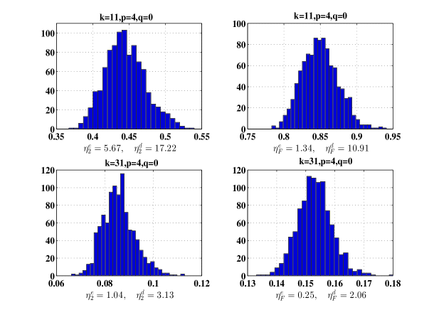
Figure 1: Approximation errors and upper bounds for a $100\times 80$ matrix whose singular values decay very slowly (decay rate: 0.9). The left figures are for the estimates of spectral errors, while the right ones correspond to the Frobenius errors.

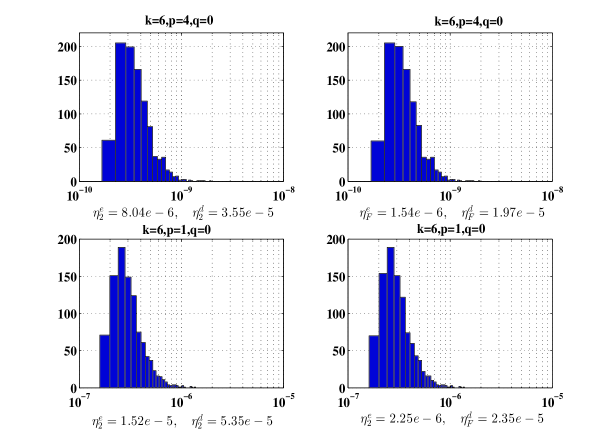
Figure 2: Approximation errors and upper bounds for a $100\times 80$ matrix whose singular values decay very fast (decay rate: 0.1) The left figures are for the estimates of spectral errors, while the right ones correspond to Frobenius errors.

In Figure 1, it is observed that for case (1) with slow decay rate in the singular values, the upper bounds $\eta_{2}^{e}$ and $\eta_{2}^{d}$ are respectively about 15 and 40 times the actual values of $\|\widehat{\bf A}_{k+p}^{(0)}-{\bf A}\|_{2}$, while for the Frobenius error $\|\widehat{\bf A}_{k+p}^{(0)}-{\bf A}\|_{F}$, the estimated upper bounds $\eta_{F}^{e}$ and $\eta_{F}^{d}$ are much tighter, and they are only about 2 and 10 times the actual values, respectively.

In Figure 2 and for case (2) with fast decay rate in the singular values, a relative large oversampling size $p=4$ gives upper bounds that are not sharp enough, and there may be a factor ${\cal O}(10^{4})$ between the estimated upper bounds and actual approximation errors. When we take $p=1$, the estimates for the upper bounds have been greatly enhanced. The reason is that the tested matrix ${\bf A}$ has fast decay rate in its singular values, therefore the orthonormal basis of ${\cal R}({\bf A\Omega})$ gives a good approximation of an $\ell$-dimensional ($\ell=k+p$) left dominant singular subspace of ${\bf A}$, which makes $\|\widehat{\bf A}_{k+p}^{(0)}-{\bf A}\|_{2}\approx\sigma_{k+p+1}$, and when $p=4$, it is much smaller than the estimated bound $\eta_{2}^{e}\approx{\cal O}(\sigma_{k+1})$.

Overall, the test results in Figures 1-2 illustrate the rationality of theoretical estimates for approximation errors.

Example 2

In this example, we test how different values of $q$ in the power scheme affect the approximation errors $\|\widehat{\bf A}_{k}^{(q)}-{\bf A}\|_{a}$. We use standard test image lena512 with $512\times 512$ pixels. This color image is characterized by a $512\times 512$ pure quaternion matrix ${\bf A}$ with entries ${\bf A}_{ij}=R_{ij}{\bf i}+G_{ij}{\bf j}+B_{ij}{\bf k}$, where $R_{ij},G_{ij},B_{ij}$ represent the red, green and blue pixel values at the location $(i,j)$ in the image, respectively. The singular values and adjacent singular value ratio ${\sigma_{k+1}/\sigma_{k}}$ of ${\bf A}$ are depicted in Figure 3.

Based on the structure-preserving quaternion Householder QR and QMGS processes for getting the orthonormal basis matrix ${\bf Q}$, we take the oversampling $p=4$ and depict the approximation errors $\|\widehat{\bf A}_{k}^{(q)}-{\bf A}\|_{a}$ for $k$ ranging from 5 to 200 with step 5 in Figures 4–5, where svdQ plots the optimal rank-$k$ approximation errors obtained via the structure-preserving QSVD algorithm wl .

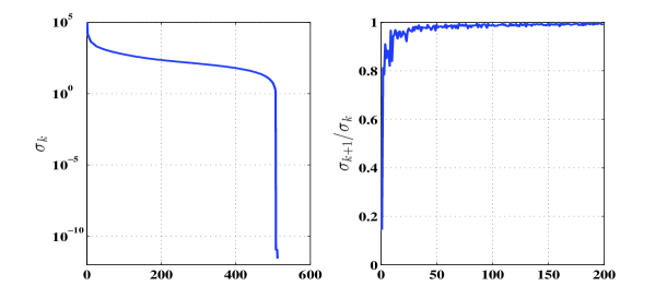
Figure 3: Singular values and adjacent singular value ratios for color image lena512.

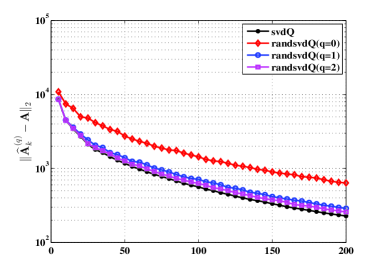
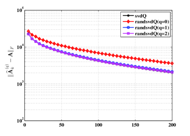
Figure 4: Errors incurred for different power schemes, in which the orthonormal basis ${\bf Q}$ in randsvdQ is obtained via quaternion Householder QR procedure.

It is observed that when $k\geq 5$, the adjacent singular value ratio is greater than 0.8, the power scheme with $q=0$ gives the worst estimates for the rank-$k$ approximation errors among three cases. In the quaternion Householder QR-based algorithm, the case with $q=2$ behaves better than that for $q=1$, since a smaller adjacent singular value ratio $\left({\sigma_{k+1}\over\sigma_{k}}\right)^{2q+1}$ of $({\bf AA}^{*})^{q}{\bf A}$ helps generate better basis matrix ${\bf Q}$ and rank-$k$ matrix approximation. Although the approximation errors from randomized algorithms are not as accurate as the svdQ-based ones, they still deliver acceptable peak signal-to-noise ratio (PNSR) and relative approximate errors as listed in Table 5.1, in which the PSNR is defined by

$${\sf PSNR}(\widehat{\bf A}_{k}^{(q)},{\bf A})=10\log_{10}{255^{2}mn\over\|\widehat{\bf A}_{k}^{(q)}-{\bf A}\|_{F}^{2}}.$$

It is observed that $q=1$ is acceptable for the desired accuracy.

Table 5.1: The peak signal-to-noise ratio and relative approximating errors for randsvdQ

$k$	$q$	PNSR	${\|\widehat{\bf A}_{k}^{(q)}-{\bf A}\|_{2}\over\|{\bf A}\|_{2}}$	${\|\widehat{\bf A}_{k}^{(q)}-{\bf A}\|_{F}\over\|{\bf A}\|_{F}}$
50	1	24.7780	0.0115	0.0602
	2	25.0501	0.0106	0.0583
100	1	29.4102	0.0057	0.0353
	2	29.7303	0.0051	0.0340
150	1	32.8041	0.0035	0.0239
	2	33.1368	0.0032	0.0230

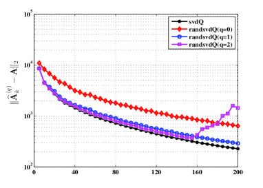
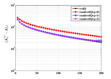
Figure 5: Errors incurred for different power schemes, in which the orthonormal basis ${\bf Q}$ in randsvdQ is obtained via quaternion MGS.

In Figure 5, QMGS-based method is compared with quaternion Householder QR procedure. QMGS gives satisfactory approximations for $k<160$ and $q=1$ or 2, while for $q=2$ and $k\geq 160$, the estimates become worse. That is partly because for $q=2$, $\left({\sigma_{1}\over\sigma_{165}}\right)^{2q+1}=1.1e+13$ and ${\bf Y}_{q}=({\bf AA}^{*})^{q}{\bf A\Omega}$ tends to be an ill-conditioned matrix, which leads to a great loss of orthogonality in the matrix ${\bf Q}$ during the QMGS procedure. However, the low-rank approximation problem only captures the dominant SVD triplets, the target rank is usually small, and in the randomized algorithm we usually deal with the QMGS of a well-conditioned matrix, the QMGS with $q=1$ is preferred, since it is more efficient than the quaternion Householder QR.

Example 3

In this example, we compare numerical behaviors of randeigQ and prandsvdQ algorithms in computing the rank-$k$ approximation of a large quaternion Hermitian matrix. It is well known that the real Laplacian matrix plays important roles in image denoising, inpainting problems for the grayscale image. Recently in ba , complex Laplacian matrix is also discussed in the mixed graph with some directed and some undirected edges, and its zero eigenvalue is proved to be related to the connection of the mixed graph. Our example involves a quaternion graph Laplacian matrix for a color image, which is modified from real hmt and complex cases.

For this purpose, we begin resizing lena512 to a $60\times 60$-pixel color image, owing to the restricted memory of Laptop. For each pixel $i$ in color channel $s\in\{r,g,b\}$, form a vector $x_{s}^{(i)}\in{\mathbb{R}}^{25}$ by gathering the 25 intensities of the pixels in a $5\times 5$ neighborhood centered at pixel $i$. Next, we form a $3600\times 3600$ pure quaternion Hermitian weight matrix ${\bf W}=W_{r}{\bf i}+W_{g}{\bf j}+W_{b}{\bf k}$ with ${\bf w}_{ji}={\bf w}_{ij}^{*}$, ${\bf w}_{ii}=0$, and ${\bf w}_{ij}=\left({w}_{r}\right)_{ij}{\bf i}+\left({w}_{g}\right)_{ij}{\bf j}+\left({w}_{b}\right)_{ij}{\bf k}$ for $i<j,$ which is determined by

$$\left(w_{s}\right)_{ij}={\rm exp}\left\{-\|x_{s}^{(i)}-x_{s}^{(j)}\|_{2}^{2}/\sigma_{s}^{2}\right\},\quad j>i,\quad s\in\{r,g,b\}.$$

Here the entries in their strictly upper triangular part of $W_{s}$ reflect the similarities between patches, and the parameter $\sigma_{s}$ controls the level of sensitivity in each channel. By zeroing out all entries of skew-symmetric matrices $W_{r},W_{g}$ and $W_{b}$ except the four largest ones in magnitude in each row, we obtain sparse weight matrices $\widetilde{W}_{s}$ and $\widetilde{\bf W}$. Similar to the complex case, let $D$ be a diagonal matrix with $d_{ii}=\sum\limits_{j}|{\bf w}_{ij}|$, and define the quaternion Laplacian matrix ${\bf L}$ as

$${\bf L}=I-D^{-1/2}\widetilde{\bf W}{D}^{-1/2}.$$

For all $s\in\{r,g,b\}$, take $\sigma_{s}=50$, store the $14400\times 3600$ real matrix ${\bf L}_{\rm c}$, and use structure-preserving algorithm eigQ jwl to compute all eigenvalues of ${\bf L}$. Here the Hermitian matrix L is a very extreme case with positive eigenvalues, and the smallest ratio ${\sigma_{k+1}/\sigma_{k}}$ of adjacent eigenvalues (singular values) of ${\bf L}$ is greater than 0.98.

Take $k=200,p=10,q=0,1,2$ to compare the eigenvalues of ${\bf L}$ via randeigQ, prandsvdQ. In all cases, the approximations of eigenvalues are not good enough, because $k=200$ only captures less than 10% proportion of eigenvalues in this extreme case, as revealed in the left figure of Figure 6. Due to the quite slow decay rate of eigenvalues, when $q$ is small, say for $q=0$, the eigenvalues computed via randeigQ, prandsvdQ are not accurate enough, but prandsvdQ still approximates eigenvalues better than randeigQ, as predicted in Remark 3. The accuracy is improved as $q$ increases, and for this extreme example, $q=2$ is sufficient to guarantee the eigenvalues from two algorithms with almost the same accuracy. For general cases, we believe that randeigQ is as reliable as prandsvdQ but more efficient for practical low-rank Hermitian matrix approximation problems with dominant singular values.

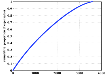
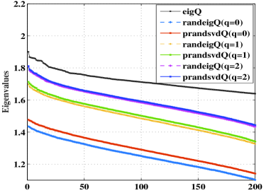
Figure 6: The cumulative proportion of eigenvalues of a quaternion Laplacian matrix and eigenvalues computed via randeigQ and prandsvdQ for $k=200,p=10$.

Example 4

In this example, we consider the color face recognition problem jns based on color principal component analysis (CPCA) approach. Suppose that there are $s$ training color image samples, denoted by $m\times n$ pure quaternion matrices ${\bf F}_{1},{\bf F}_{2},\ldots,{\bf F}_{s},$ and the average is ${\bf\Psi}={1\over s}\sum\limits_{t=1}^{s}{\bf F}_{t}\in{\mathbb{Q}}^{m\times n}$. Let ${\bf X}=[{\rm vec}({\bf F}_{1})-{\rm vec}({\bf\Psi}),\cdots,{\rm vec}({\bf F}_{s})-{\rm vec}({\bf\Psi})],$ where ${\rm vec}(\cdot)$ means to stack the columns of a matrix into a single long vector. The core work of CPCA approach is to compute the left singular vectors corresponding to the first $k$ largest singular values of ${\bf X}$, which are called the eigenfaces. The eigenfaces can also be obtained from the eigQ algorithm jwl applied to ${\bf XX}^{*}$ or ${\bf XX}^{*}$.

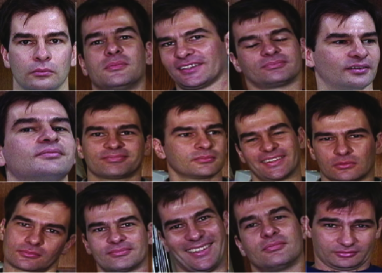
Figure 7: Sample images for one individual of the Georgia Tech face database

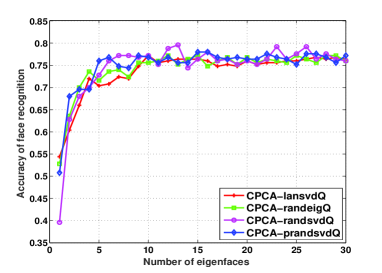
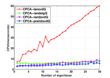
Figure 8: The color face recognition accuracy and CPU time by lansvdQ, randsvdQ, randeigQ and prandsvdQ methods with parameters $p=4,q=0$.

For color image samples, we use the Georgia Tech face database, and all images are manually cropped, and then resized to $120\times 120$ pixels. The samples of the cropped images are shown in Figure 7. There are 50 persons to be used. The first ten face images per individual person are chosen for training and the remaining five face images are used for testing. The number of chosen eigenfaces, $k$, increases from 1 to 30. We need to compute $k$ SVD triplets of a $14400\times 500$ quaternion matrix ${\bf X}$, in which the 14400 rows refer to $120\times 120$ pixels and the 500 columns refer to 50 persons with 10 faces each.

As revealed in jns , the matrix is very large and the svdQ algorithm does not finish the computation of the singular value decomposition of ${\bf X}$ in 2 hours and eigQ needs about seven times of the running CPU time via the quaternion Lanczos-based algorithm (lansvdQ). In this experiment we consider the lansvdQ, randsvdQ, prandsvdQ algorithms of ${\bf X}$, and randeigQ algorithm of ${\bf X^{*}X}$, where the orthonormal basis is derived based on quaternion MGS process, and in randeigQ, the matrix ${\bf X^{*}X}$ is not explicitly formed. The detailed comparisons of recognition accuracy and running CPU time of candidate methods are depicted in Figure 8, in which the accuracy of face recognition is the percentage of correctly recognized persons for given 250 test images. For $p=4$ and $q=0$, randomized algorithms have higher recognition accuracy than lansvdQ, and are much more efficient than lansvdQ. Moreover, the preconditioning technique for randsvdQ can slightly enhance the efficiency of the algorithm. Unlike lansvdQ, the CPU time for randomized algorithms does not increase significantly with the target rank (number of eigenfaces). lansvdQ is much less efficient partly because it uses for-end loop and performs matrix-vector products at each iteration, while the randomized algorithms make full use of the matrix-matrix products that have been highly optimized for maximum efficiency on modern serial and parallel architectures gv2 .

Example 5

In this example, we generalize the fast frequent directions via subspace embedding (SpFD) method tc to the quaternion case. The corresponding algorithm is referred to as SpFDQ, and is compared with prandsvdQ through the color face recognition problem in Example 4.

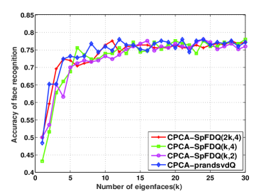
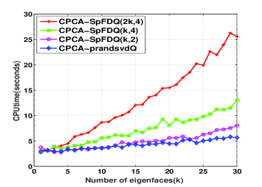
Figure 9: The color face recognition accuracy and CPU time by SpFDQ($\ell,t$) and prandsvdQ methods with parameters $p=4,q=0$.

Given a real matrix $A\in{\mathbb{R}}^{m\times n}$ ($m\geq n$), the SpFD($\ell,t$) algorithm squeezes the rows of $A$ by pre-multiplying $SP$ on $A$, where $t$ is assumed to be a factor of $m$ (if not, append zero rows to the end of $A$ until $m$ is), $P$ is a random permutation matrix, and $S={\rm diag}(S_{1},\ldots,S_{t})$ is a sparse sketching matrix with $S_{i}\in{\mathbb{R}}^{\ell\times{m\over t}}$ being generated on a probability distribution. At the start of the algorithm, it extracts and shrinks the top $\ell$ important right singular vectors of a two-layered matrix $\Big{[}{S_{1}PA\atop S_{2}PA}\Big{]}$ via SVD, and then combines them with the next $\ell$ rows in $SPA$ to form a new two-layered matrix. Repeat the procedure until the last $\ell$ rows of $SPA$ is combined into the computation. Finally, an orthonormal basis $V_{\ell}\in{\mathbb{R}}^{n\times\ell}$ for the row space of $SPA$ is obtained, and a rank-$k$ approximation of $A$ is derived based on the SVD of $AV_{\ell}$. The algorithm consists of $(t-1)$ iterations, and the total cost is

$$2{\rm nnz}(A)(\ell+1)+[24n\ell^{2}+160\ell^{3}](t-1)+6m\ell^{2}+20\ell^{3}+2m\ell k+2mn\ell,\quad t>1,$$

where $m\geq n\geq\ell\geq k$, $m\gg\ell$. The choice of $t=2,\ell=k$ corresponds to an algorithm with the cheapest cost, while for $t=\lceil m/\ell\rceil$, SpFD($\ell,t$) reduces to a slight modification of FD in glp .

In the SpFDQ($\ell,t$) algorithm, ${\bf A}$ is taken to be the $14400\times 500$ matrix ${\bf X}$ in Example 4, and the choice of sketching matrix $S$ is the same as the real case. To perform a fair comparison, we also consider the preconditioned technique in the QSVD of a short-and-wide or tall-and-narrow quaternion matrix. During the $(t-1)$ rounds of QSVD in the iteration, due to the potential singularity of the sketching matrix $S_{i}$ that might lead to a singular two-layered matrix, we apply quaternion Householder QR first and then implement the QSVD on a small-size matrix. In the last round of QSVD of ${\bf AV}_{\ell}$, the QSVD of ${\bf AV}_{\ell}$ is obtained via the QMGS of ${\bf AV}_{\ell}$ first and then applying QSVD to a small upper triangular factor.

The accuracy of face recognition and running CPU time of SpFDQ($\ell,t$) and prandsvdQ algorithms are shown in Figure 9. The depicted results demonstrate that SpFDQ($k,2$) is the most efficient one among all SpFDQ($\ell,t$) algorithms, while prandsvdQ is a little more efficient than SpFDQ($k,2$) when $k$ increases. For the recognition accuracy, prandsvdQ has higher recognition accuracy for most parameter values of $k$, while there also exists a parameter, say for $k=22$, prandsvdQ has lower recognition accuracy than other candidate methods. That is partly because the sketching matrix $S$ and random ${\bf\Omega}$ are randomly generated on specific distributions, and the recognition accuracy is sometimes affected by the properties of some specific random matrices.

In order to perform a fair comparison, in Table 5.2 we execute each algorithm 20 times, and display the average (avrg), maximal (max) and minimal (min) numbers of correctly recognized persons among 250 test faces for 50 persons, and the average running CPU time (avtime) is also given. It is observed that when $k$ is small, say for $k\leq 9$, there exist big fluctuations on the recognition accuracy of SpFDQ($k$,2), and the average numbers of recognized faces increase when the sketching size in SpFDQ($2k$,2) is increased, but SpFDQ($2k$,2) still has lower recognition accuracy than prandsvdQ. When $k$ increases, the difference of face recognition accuracy becomes smaller, while for the running time, prandsvdQ is the most efficient.

Table 5.2: Comparisons of SpFDQ($\ell$,2) with prandsvdQ for PCA-based color image recognition problems

SpFDQ($k$,2)
$k$	3	6	9	12	15	18	21	24	27	30
avrg	153.25	178.65	184.70	188.05	189.80	189.85	190.00	190.80	190.95	192.40
max	184	188	191	194	195	193	195	195	195	196
min	130	169	176	182	183	185	184	187	187	187
avtime	2.97	3.29	3.68	4.10	4.63	5.47	5.62	6.02	6.86	7.45
SpFDQ($2k$,2)
$k$	3	6	9	12	15	18	21	24	27	30
avrg	161.35	178.75	184.85	190.30	189.25	190.00	188.95	190.60	190.85	191.80
max	172	186	190	194	192	192	192	193	196	196
min	150	172	180	186	186	187	186	188	186	188
avtime	3.18	3.92	4.72	5.60	6.96	7.91	9.27	10.47	12.09	13.56
prandsvdQ
$k$	3	6	9	12	15	18	21	24	27	30
avrg	174.35	187.10	190.55	191.30	190.65	191.15	192.65	193.45	192.25	192.85
max	182	195	201	198	194	198	196	198	197	197
min	164	182	183	185	185	184	187	188	188	189
avtime	3.02	3.30	3.44	3.70	4.11	4.44	4.73	5.02	5.50	5.82

6 Conclusion

In this paper we have presented the randomized QSVD algorithm for quaternion low-rank matrix approximation problems. For large scale problems with a small target rank, the randomized algorithm compresses the size of the input matrix by the quaternion normal distribution-based random sampling, and approximates dominant SVD triplets with good accuracy and high efficiency. The approximation errors of the randomized algorithm are illustrated by the detailed theoretical analysis and numerical examples. Compared to the Lanczos-based QSVD (lansvdQ) and fast frequent direction via subspace embedding (SpFDQ) algorithms, the randomized algorithms display their effectiveness and efficiency for PCA-based color image recognition problems.

Acknowledgments. The authors are grateful to the handling editor and three anonymous referees for their useful comments and suggestions, which greatly improved the original presentation.

References

- (1) R. B. Bapat, D. Kalita and S. Patib, On weighted directed graphs, Linear Algebra Appl., 436 (2012), pp. 99-111.
- (2) N. L. Bihan and S. J. Sangwine, Quaternion principal component analysis of color images, IEEE International Conference on Image Processing, 1 (2003), pp. 809-812.
- (3) Z. Z. Chen and J. J. Dongarra, Condition numbers of Gaussian random matrices, SIAM J. Matrix Anal. Appl., 27 (2005), pp. 603-620.
- (4) K. L. Clarkson and D. P. Woodruff, Numerical linear algebra in the streaming model, STOC ‘09: Proc. 41st Ann. ACM 476 Symp. Theory of Computing, 2009.
- (5) J. A. Duersch and M. Gu, Randomized projection for rank-revealing matrix factorizations and low-rank approximations, SIAM Rev., 62 (2020), pp. 661-682.
- (6) T. A. Ell, N. L. Bihan and S. J. Sangwine, Quaternion Fourier Transforms for Signal and Image Processing, Wiley, Hoboken, NJ, USA, 2014.
- (7) M. Ghashami, E. Liberty, J. M. Phillips and D. P. Woodruff, Frequent directions: simple and deterministic matrix sketching, SIAM J. Comput., 45 (2016), pp. 1762-1792.
- (8) G. H. Golub and C. F. Van Loan, Matrix Computations(4ed.), Johns Hopkins University Press, Baltimore, 2013.
- (9) G. H. Golub and C. Reinsch, Singular value decomposition and least squares solutions, Numer. Math., 14 (1970), pp. 403-420.
- (10) M. Gu, Subspace iteration randomization and singular value problems, SIAM J. Sci. Comput., 37 (2015), A1139-A1173.
- (11) N. Halko, P. G. Martinsson and J. A. Tropp, Finding structure with randomness: probabilistic algorithms for constructing approximate matrix decompositions, SIAM Rev., 53 (2011), pp. 217-288.
- (12) W. R Hamilton, Elements of Quaternions, Chelsea, New York, 1969.
- (13) Z. G. Jia, M. S. Wei and S. T. Ling, A new structure-preserving method for quaternion Hermitian eigenvalue problems, J. Comput. Appl. Math., 239 (2013), pp. 12-24.
- (14) Z. G. Jia, M. S. Wei, M. X. Zhao and Y. Chen, A new real structure-preserving quaternion QR algorithm, J. Comput. Appl. Math., 343 (2018), pp. 26-48.
- (15) Z. G. Jia, M. K. Ng and G. J. Song, Lanczos method for large-scale quaternion singular value decomposition, Numer. Algorithms, 82 (2019), pp. 699-717.
- (16) Z. G. Jia, M. K. Ng and G. J. Song, Robust quaternion matrix completion with applications to image inpainting, Numer. Linear Algebra Appl., 26 (2019), e2245.
- (17) Z. G. Jia, M. K. Ng and W. Wang, Color image restoration by saturation-value (SV) total variation, SIAM J. Imag. Sci., 12 (2019), pp. 972-1000.
- (18) Z. G. Jia, The Eigenvalue Problem of Quaternion Matrix: Structure-Preserving Algorithms and Applications, Science Press, Beijing, 2019.
- (19) Z. G. Jia and M. K. Ng, Structure preserving quaternion generalized minimal residual method, SIAM J. Matrix Anal. Appl., 42 (2021), pp. 616-634.
- (20) S. M. Li, A theory of statistical analysis based on normal distrubution of quaternion (in Chinese), Ph.D Thesis, Sun Yat-sen University, 2001.
- (21) Y. Li, M. S. Wei, F. X. Zhang and J. L. Zhao, Real structure-preserving algorithms of Householder based transformations for quaternion matrices, J. Comput. Appl. Math., 305 (2016), pp. 82-91.
- (22) Y. Li, M. S. Wei, F. X. Zhang and J. L. Zhao, A structure-preserving method for the quaternion LU decomposition, Calcolo, 54 (2017), pp. 1553-1563.
- (23) E. Liberty, F. Woolfe, P. Martinsson, V. Rokhlin and M. Tygert, Randomized algorithms for the low-rank approximation of matrices, Proceedings of the National Academy of Sciences, 104 (2007), pp. 20167-20172.
- (24) M. T. Loots, On the development of the quaternion normal distribution, Master Thesis, University of Pretoria, Pretoria, 2010.
- (25) M. W. Mahoney, Randomized algorithms for matrices and data, Foundations and Trends in Machine Learning, 3 (2011), pp. 123-224.
- (26) P. G. Martinsson, V. Rokhlin and M. Tygert, A randomized algorithm for the decomposition of matrices, Appl. Comput. Harmon. Anal., 30 (2011), pp. 47-68.
- (27) X. Meng and M.W. Mahoney, Low-distortion subspace embeddings in input-sparsity time and applications to robust linear regression, Proc. 45th Annu. ACM Symp. Theory Comput., 2013, pp. 91-100.
- (28) T. Minemoto, T. Isokawa, H. Nishimura and N. Matsui, Feed forward neural network with random quaternionic neurons, Signal Processing, 136 (2017), pp. 59-68.
- (29) R. J. Muirhead, Aspects of Multivariate Statistical Theory, Wiley, New York, NY, 1982.
- (30) L. Rodman, Topics in Quaternion Linear Algebra, Princeton University Press, 2014.
- (31) B. J. Saap, Randomized algorithms for low rank matrix decomposition, Technical Report, Computer and Information Science, University of Pennsylvania, 2011.
- (32) S. J. Sangwine and N. L. Bihan, Quaternion singular value decomposition based on bidiagonalization to a real or complex matrix using quaternion Householder transformations, Appl. Math. Comput. 182 (2006), pp. 727-738.
- (33) T. Sarls, Improved approximation algorithms for large matrices via random projections, Proc. 47th Annu. IEEE Symp. Foundations Comput. Sci., 2006, pp. 143-152.
- (34) D. Teng and D. L. Chu, A fast frequent directions algorithm for low rank approximation, IEEE Trans. Pattern Anal. Mach. Intell., 41 (2019), pp. 1279-1293.
- (35) C. Y. Teng and K. T. Fang, Statistical analysis based on normal distribution of quaternion, International Symposium on Contemporary Multivariate Analysis and its Applications, 1997.
- (36) C. Y. Teng and S. M. Li, Exterior differential form on quaternion matrices and its application (in Chinese), Acta Scientiarum Naturalium Universitatis SunYatseni, 38 (1999), pp. 12-16.
- (37) M. H. Wang, W. H. Ma, A structure-preserving method for the quaternion LU decomposition in quaternionic quantum theory, Comput. Phys. Comm., 184 (2013), pp. 2182-2186.
- (38) M. S. Wei, Y. Li, F. X. Zhang, J. L. Zhao, Quaternion Matrix Computations, Nova Science Publishers, 2018.
- (39) F. Woolfe, E. Liberty, V. Rokhlin and M. Tygert, A fast randomized algorithm for the approximation of matrices, Appl. Comput. Harm. Anal., 25 (2008), pp. 335-366.
- (40) W. J. Yu, Y. Gu and Y. H. Li, Efficient randomized algorithms for the fixed-precision low-rank matrix approximation, SIAM J. Matrix Anal. Appl., 39 (2018), pp. 1339-1359.
- (41) F. Z. Zhang, Quaternions and matrices of quaternion, Linear Algebra Appl., 251 (1997), pp. 21-57.
- (42) L. P. Zhang and Y. M. Wei, Randomized core reduction for discrete ill-posed problem, J. Comput. Appl. Math., 375 (2020), 112797.
- (43) M. X. Zhao, Z. G. Jia, Y. F. Cai, X. Chen and D. W. Gong, Advanced variations of two-dimensional principal component analysis for face recognition, Neurocomputing, 452 (2021), pp. 653-664.