A Sub-Element Adaptive Shock Capturing Approach for Discontinuous Galerkin Methods

Abstract

In this paper, a new strategy for a sub-element based shock capturing for discontinuous Galerkin (DG) approximations is presented. The idea is to interpret a DG element as a collection of data and construct a hierarchy of low to high order discretizations on this set of data, including a first order finite volume scheme up to the full order DG scheme. The different DG discretizations are then blended according to sub-element troubled cell indicators, resulting in a final discretization that adaptively blends from low to high order within a single DG element. The goal is to retain as much high order accuracy as possible, even in simulations with very strong shocks, as e.g. presented in the Sedov test. The framework retains the locality of the standard DG scheme and is hence well suited for a combination with adaptive mesh refinement and parallel computing. The numerical tests demonstrate the sub-element adaptive behavior of the new shock capturing approach and its high accuracy.

1 Introduction

For non-linear hyperbolic problems, such as the compressible Euler equations, there are two major sources of instabilities when applying discontinuous Galerkin (DG) methods as a high order spatial discretization. (i) Aliasing is caused by under-resolution of e.g. turbulent vortical structures and can lead to instabilities that may even crash the code. As a cure, de-aliasing mechanisms are introduced in the DG methodology based on e.g. filtering [31, 30], polynomial de-aliasing [37, 58, 38] or analytical integration [32, 26], split forms of the non-linear terms that for instance preserve kinetic energy [62, 23, 25, 18], and entropy stability [5, 61, 48, 7, 47, 45, 6, 46, 44, 3, 27, 22, 20]. (ii) The second major source of instabilities is the Gibbs phenomenon, i.e. oscillations at discontinuities. It is well known that solutions of non-linear hyperbolic problems may develop discontinuities in finite time, so called shocks. While aliasing issues can be mostly attributed to variational crimes, i.e. a bad design and implementation of the numerical discretization with simplifications that affects aliasing (e.g. collocation), oscillations at discontinuities have their root deeper in the innards of the high order DG approach and are unfortunately an inherent property of the high order polynomial approximation space. Oscillations are fatal when physical constraints and bounds on the solution exist that then break because of over- and undershoots, resulting in nonphysical solutions such as negative density or pressure.

In this work, we focus on a remedy for the second major stability issue, often referred to as shock capturing. There are many shock capturing approaches available in DG literature, for instance based on slope limiters [11, 10, 41] or (H)WENO limiters [28, 51, 66], filtering [2], and artificial viscosity [49, 9]. Slope limiters or (H)WENO limiters are always applied in combination with troubled cell indicators that detect shocks and only flag the DG elements that are affected by oscillations. Only in these elements, the DG polynomial is replaced by an oscillation free reconstruction using data from neighboring elements. Element based slope limiting, e.g., with TVB limiters is effective for low order DG discretizations only, as its accuracy strongly degrades when increasing the polynomial order $N$, as in some sense the size of the DG elements $\Delta x$ gets larger and larger with higher polynomial degree $N$. The accuracy of the slope limiters is not based on the DG resolution $\sim\frac{\Delta x}{N}$, but only on the element size $\Delta x$. Considering that a finite volume (FV) discretization with high order reconstructions and limiters typically resolve a shock within about 2-3 cells, the shock width for high order DG schemes with large elements would be very wide when relying on element based limited reconstructions. The same behavior is still an issue for high order reconstruction based limiters such as the (H)WENO methodology. While these formally use high order reconstructions, its leading discretization parameter is still $\Delta x$ and not $\frac{\Delta x}{N}$ and hence the shock width still scales with $\Delta x$.

Sub-element resolution, i.e. a numerical shock width that scales proportional to $\frac{\Delta x}{N}$, can be achieved with e.g. artificial viscosity. The idea is to widen the discontinuity into a sharp, but smooth profile such that high order polynomials can resolve it. Again, some form of troubled cell indicator is introduced to not only flag the element that contains the shock (or that oscillates) but also determine the amount of necessary viscosity, e.g., based on local entropy production [67]. It is interesting that less viscosity is needed, i.e. sharper shock profiles are possible, the higher the polynomial degree of the DG discretization. Shocks can be captured in a single DG element if the polynomial order is high enough [49]. An issue of artificial dissipation is that a high amount of artificial viscosity is needed for very strong shocks, which makes the overall discretization very stiff with a very small explicit time step restriction. Local time stepping can be used to reduce this issue [24] or specialized many stage Runge-Kutta schemes with optimized coefficients for strongly dissipative operators [33].

An alternative idea to achieve sub-element resolution is to actually replace the elements by sub-elements (lower order DG on finer grid) or maybe even finite volume (FV) subcells. A straight forward, maybe even a natural idea in the DG methodology is to use hp-adaptivity, where the polynomial degree is reduced and simultaneously the grid resolution is increased close to discontinuities. When switching to the lowest order DG, i.e a first order DG, which is nothing but a first order FV method, it is assumed that the inherent artificial dissipation of the first order FV scheme is enough to clear all oscillations at even the strongest shocks. The low accuracy of the first order FV method is compensated by a respective (very strong) increase in local grid resolution through h-adaptivity. An obvious downside to the hp-adaptivity approach is the strong dynamic change of the approximation space during the simulation and the associated strong change of the underlying data structures.

Thus, as a simpler alternative, subcell based FV discretizations with a first order, second order TVD or high order WENO reconstruction was introduced, e.g., in [60, 57, 15, 63, 14]. The idea is to completely switch the troubled DG element to a robust FV discretization on a fine subcell grid. This approach keeps the change of the data local to the affected DG element and helps to streamline the implementation. The robust and essential oscillation free FV scheme on the finer subcell grid in the DG element is constructed based on the available DG data. This helps to keep the data structures feasible and reduces the shock capturing again to an element local technique instead of changing the global mesh topology and approximation space. Consequently, this again allows to combine the approach with the idea of a troubled cell mechanism to identify the oscillatory DG elements and replace the high order DG update with the robust FV update. As noted, there are many different variants for the FV subcell scheme with the high order WENO [60, 57, 15, 63, 14] variant being especially interesting, as it alleviates the ’stress’ on the troubled cell indicator. When accidentally switching the whole high order DG element to the subcell FV scheme in smooth parts of the solution, accuracy may strongly degrade. A first order FV scheme, even on the fine subcell grid, would wash away all fine structure details that the high order DG approach simulated. Thus, from this point of view, a high order subcell WENO FV scheme is highly desired in this context. A downside of a subcell WENO FV scheme is the non-locality of the data dependence due to the high order reconstruction stencils. This is especially cumbersome close to the interface of the high order DG elements, where the reconstruction stencils reach into the neighboring DG elements and thus fundamentally change the data dependency footprint of the resulting implementation, that consequently has a direct impact on the parallelization of the code.

In this paper, the goal is to augment a high order DG method with sub-element shock capturing capabilities to allow the robust simulation of highly supersonic turbulent flows which feature strong shocks, as e.g. in astrophysics, without changing the data dependency footprint. Instead of flagging an element and completely switching from the high order DG scheme to the subcell FV scheme, we aim to smoothly combine different schemes in the flagged element. To achieve this, we firstly interpret the DG element as a collection of available mean value data. As depicted in Fig.1, local reconstructions allow to define a hierarchy of approximation spaces, from pure piecewise constant approximations (subcell FV) up to a smooth global high order polynomial (DG element), with all piecewise polynomial combinations (sub-element DG) in between. We then associate each possible approximation space with the corresponding FV or DG discretization to define a hierarchy of schemes that is available for the given collection of data.

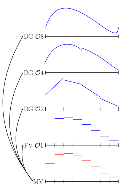
Figure 1: Sketch of the main idea in a one-dimensional setting. Starting with eight mean values (red), we interpret them as a collection of available data. We construct four different approximation spaces (blue): piecewise constant on a subcell grid, piecewise linear and piecewise cubic on a sub-element grid, and the full 7th degree polynomial on the element.

Instead of switching between these different schemes, we aim to smoothly blend them in order to achieve the highest possible accuracy in every DG element. Assuming that the first order subcell FV approximation has enough inherent dissipation to capture shocks in an oscillation free manner, the goal is to give the FV discretization a high enough weight at a shock and then smoothly transition to higher order (sub-element) DG away from the shock. In contrast to the common approaches, where one indicator is used for the whole DG element, we aim to introduce sub-element indicators that are adaptively adjusted inside the DG element. A difficulty that arises when using sub-element indicators and an adaptive blending approach is to retain conservation of the final discretization for arbitrary combinations of blending weights.

The final discretization is a blended scheme, where the weights of the different discretizations may vary inside the DG element. To demonstrate this idea, the resulting behavior of the new approach is depicted in Fig. 2 for the example of a Sedov blast wave in 2D. In this particular setup, we start with 8th order DG as our baseline high order discretization. The grey grid lines indicate the 8th order DG element borders. Re-interpreting the 2D 8th order DG element as $8^{2}$ mean value data, we can construct either a first order FV scheme on $8^{2}$ subcells, a fourth order DG scheme on $2^{2}$, or a second order DG scheme on $4^{2}$ sub-elements. The blending of the four available discretizations is visualized via a weighted blending factor (introduced in equation (57)) in Fig. 2 ranging from $1$ (dark red, basically pure first order FV) up to $8$ (dark blue, basically pure 8th order DG) and all combinations in between.

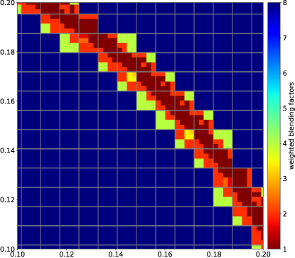
Figure 2: Visualization of the sub-element adaptive blending approach for the 2D Sedov blast wave, see Sec. 3 for a detailed discussion. The gray grid lines represent the 8th order DG elements. The color represents the blending process, where dark red (value $1$) corresponds to pure first order FV and dark blue (value $8$) corresponds to the pure 8th order DG scheme, with all combination in between. Note, that the plotted value is only for illustration and does not correspond to an actual mixed mathematical order of the final discretization. But the value nicely illustrates how even inside a DG element, the discretization is adaptively adjusted.

Clearly, the new approach adaptively changes on a sub-element level with a very localized low order near the shock front, while a substantial part of the high order DG approximation is recovered away from the shock. We refer to the validation and application sections, Sec. 3 and Sec. 4, for a more detailed discussion.

The remainder of the paper is organized as follows: in Sec. 2 we introduce the numerical scheme with the blending of the different discretizations. Sec. 3 include numerical validations and Sec. 4 shows an application of the presented approach with the conclusion given in the last section.

2 The Sub-Element Adaptive Blending Approach

The derivations in sections 2.1-2.6 are done in 1D, where the domain $\Omega$ is divided into $Q$ non-overlapping elements. Each element $q$ with midpoint $x_{q}$ and size $\Delta x_{q}$ is mapped to the reference space as

$$x(\chi)=x_{q}+\chi\,\Delta x_{q}\,,\quad\chi\in\left[-\frac{1}{2},\frac{1}{2}\right].$$ (1)

Each element holds a total number of degrees of freedom (DOF) $N$, where we require $N\in\{2^{r},r\in\mathbb{N}\}$. For the FV method, the element is divided into $N$ subcells of size $\frac{\Delta x_{q}}{N}$ leading to a uniform grid with midpoints $\mu_{i}$ and interfaces $\mu_{i\pm\frac{1}{2}}$ in the reference space at

$$\mu_{i}=-\frac{1}{2}+\frac{i}{N}-\frac{1}{2\,N}\quad\text{and}\quad\mu_{i\pm\frac{1}{2}}=\mu_{i}\pm\frac{1}{2\,N},\quad i=1,\ldots,N.$$ (2)

For the sub-element DG scheme of order $n=2^{r}<N,r\in\mathbb{N}$, the element is divided into $\frac{N}{n}$ uniform sub-elements of size $\frac{n\Delta x_{q}}{N}$, and the mapping of each sub-element $s$ to its (sub-)reference space reads as

$$\chi(\xi)_{s}^{\mathcal{O}(n)}=-\frac{1}{2}+\frac{s\,n}{N}-\frac{n}{2\,N}+\frac{n}{N}\xi,\quad s=1,\dots,\frac{N}{n},\;\xi\in\left[-\frac{1}{2},\frac{1}{2}\right].$$ (3)

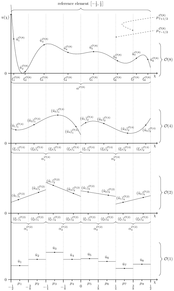
Figure 18: Schematic of eight ($N=8$) mean values and its four levels of data interpretation. The values $\mu_{7\pm 1/2}^{\mathcal{O}(8)}$ indicate the location of the interpolation nodes in (48) of the FV subcell interpolation operator $\bm{I}^{\pm\mathcal{O}(n)}$, $n=2,4,8$.

Fig. 18 in appendix 6.1 provides a visual representation of the reference element and its hierarchical decomposition into sub-elements and subcells.

2.1 Finite Volume Method

Consider the general 1D conservation law

$$\partial_{t}u+\partial_{x}f(u)=0.$$ (4)

We approximate the exact solution $u(x)$ in element $q$ with $N$ mean values

$$\bm{\bar{u}}_{q}=(\bar{u}_{1},\ldots,\bar{u}_{N})_{q}^{T}\;\in\mathbb{R}^{N},$$ (5)

residing on the uniform subcell grid (2). Then the 1D FV semi-discretization on subcell $i$ reads

$$\big{(}\partial_{t}\bar{u}_{i}\big{)}_{q}=-\frac{N}{\Delta x_{q}}\,\Big{(}f^{*}\big{(}(\bar{u_{i}})_{q},(\bar{u}_{i+1})_{q}\big{)}-f^{*}\big{(}(\bar{u}_{i-1})_{q},(\bar{u}_{i})_{q}\big{)}\Big{)},\quad i\in 1,\ldots,N,$$ (6)

where $f^{*}$ denotes a consistent numerical two point flux. The adjacent values from neighboring elements $q-1$ and $q+1$ are given by $(\bar{u}_{0})_{q}:=(\bar{u}_{N})_{q-1}$ and $(\bar{u}_{N+1})_{q}:=(\bar{u}_{1})_{q+1}$. We define the Finite Volume Difference Matrix

$$\bm{\Delta}:=\begin{pmatrix}-1&1&0&\cdots&0\\ 0&-1&1&\ddots&\vdots\\ \vdots&\ddots&\ddots&\ddots&0\\ 0&\cdots&0&-1&1\end{pmatrix}\in\mathbb{R}^{N\times(N+1)},$$ (7)

and rewrite (6) in compact matrix form

$$\partial_{t}\bm{\bar{u}}_{q}=-\frac{N}{\Delta x_{q}}\,\bm{\Delta}\,\bm{f}_{q}^{*},$$ (8)

with the numerical flux vector $\bm{f}_{q}^{*}\in\mathbb{R}^{N+1}$. For later use we split $\bm{\Delta}$ into a volume and a surface operator:

$$\bm{\Delta}=\bm{\Delta}^{(V)}+\bm{\Delta}^{(S)}=\begin{pmatrix}0&1&0&\cdots&0\\ 0&-1&1&\ddots&\vdots\\ \vdots&\ddots&\ddots&\ddots&0\\ 0&\cdots&0&-1&0\end{pmatrix}+\begin{pmatrix}-1&0&0&\cdots&0\\ 0&0&0&\ddots&\vdots\\ \vdots&\ddots&\ddots&\ddots&0\\ 0&\cdots&0&0&1\end{pmatrix}.$$ (9)

Remark: The FV volume operator vanishes when summed along columns, i.e.

$$\bm{1}^{T}\,\bm{\Delta}^{(V)}=\bm{0}^{T},$$ (10)

where $\bm{1}=(1,\ldots,1)^{T}\in\mathbb{R}^{N}$ is the vector of ones.

2.2 Discontinuous Galerkin Method

In this section we briefly outline the Discontinuous Galerkin Spectral Element Method (DGSEM) [1, 36]. To derive the $n$-th order DG scheme within sub-element $s$, (eq. (3)) residing inside element $q$, we first rewrite the conservation law (4) into variational form with a test function $\phi$ and apply spatial integration-by-parts to the flux divergence

$$\int_{\Omega_{s}}\partial_{t}u_{q}\,\phi\,d\xi=\frac{N}{n\,\Delta x_{q}}\left(\int_{\Omega_{s}}f(u_{q})\,\partial_{\xi}\phi\,d\xi-f^{*}(u_{q})\,\phi\big{|}_{\partial\Omega_{s}}\right).$$ (11)

We choose the test functions $\phi$ as Lagrange functions

$$\ell_{i}(\xi)=\prod^{n}_{k=1,k\neq i}\frac{\xi-\xi_{k}}{\xi_{i}-\xi_{k}},\quad i=1,\dots,n,$$ (12)

spanned with the collocation nodes $\xi_{i}\in\left[-\tfrac{1}{2},\tfrac{1}{2}\right]$, and use the polynomial ansatz

$$u(t;\xi)\approx\sum_{i=1}^{n}\tilde{u}_{i}(t)\,\ell_{i}(\xi)=\bm{\tilde{u}}^{T}(t)\,\bm{\ell}(\xi),$$ (13)

where

$$\bm{\tilde{u}}(t)=\big{(}\tilde{u}_{1}(t),\ldots,\tilde{u}_{n}(t)\big{)}^{T}\quad\text{and}\quad\bm{\ell}(\xi)=\big{(}\ell_{1}(\xi),\ldots,\ell_{n}(\xi)\big{)}^{T}$$ (14)

are the vectors of nodal coefficients and Lagrange polynomials. We use collocation of the non-linear flux functions with the same polynomial approximation. Numerical quadrature is collocated as well. The nodes are the Gauss-Legendre quadrature nodes. These quadrature nodes and the interpolation polynomials are also illustrated in Fig. 18 in the appendix 6.1.

Inserting everything into (11) gives the semi-discrete weak-form DG scheme

$$\bm{\mathcal{M}}\,\partial_{t}\bm{\tilde{u}}_{s}=\frac{N}{n\,\Delta x_{q}}\left(\bm{\mathcal{D}}^{T}\bm{\mathcal{M}}\,\bm{\tilde{f}}_{s}-\bm{\mathcal{B}}\,\bm{f}_{s}^{*}\right).$$ (15)

The diagonal mass matrix is

$$\left(\bm{\mathcal{M}}\right)_{ij}=\delta_{ij}\,\omega_{i},$$ (16)

with associated numerical quadrature weights $\omega_{i}$, and the differentiation matrix is

$$\left(\bm{\mathcal{D}}\right)_{ij}=\partial_{\xi}\ell_{j}(\xi)\big{|}_{\xi_{i}}.$$ (17)

The DG volume flux $\bm{\tilde{f}}_{s}$ is computed directly with the nodal values $\bm{\tilde{u}}_{s}$ of the polynomial ansatz (13)

$$\bm{\tilde{f}}_{s}=f\left(\bm{\tilde{u}}_{s}\right):=\Big{(}f\big{(}(\tilde{u}_{1})_{s}\big{)},\ldots,f\big{(}(\tilde{u}_{n})_{s}\big{)}\Big{)}^{T}\;\in\mathbb{R}^{n},$$ (18)

and the surface flux vector

$$\bm{f}_{s}^{*}=\Big{(}f^{*}(\underbrace{\tilde{u}_{s-1}^{+},\tilde{u}_{s}^{-}}_{\mathclap{\begin{subarray}{c}\text{left sub-element}\\ \text{interface}\end{subarray}}}),0,\ldots,0,f^{*}(\underbrace{\tilde{u}_{s}^{+},\tilde{u}_{s+1}^{-}}_{\mathclap{\begin{subarray}{c}\text{right sub-element}\\ \text{interface}\end{subarray}}})\Big{)}^{T}\;\in\mathbb{R}^{n}$$ (19)

is constructed with the numerical flux evaluated at DG sub-element boundaries

$$\tilde{u}_{s}^{+}=(\bm{b}^{+})^{T}\,\bm{\tilde{u}}_{s}\quad\text{and}\quad\tilde{u}_{s}^{-}=(\bm{b}^{-})^{T}\,\bm{\tilde{u}}_{s},$$ (20)

where $\bm{b}^{\pm}$ are the boundary interpolation operators

$$\bm{b}^{\pm}=\Big{(}\ell_{1}\big{(}\pm\tfrac{1}{2}\big{)},\ldots,\ell_{n}\big{(}\pm\tfrac{1}{2}\big{)}\Big{)}^{T}\;\in\mathbb{R}^{n}.$$ (21)

The boundary evaluation operator can be compactly written as

$$\bm{\mathcal{B}}=\begin{pmatrix}-\ell_{1}(-\tfrac{1}{2})&0&\cdots&0&\ell_{1}(\tfrac{1}{2})\\ \vdots&\vdots&\ddots&\vdots&\vdots\\ -\ell_{n}(-\tfrac{1}{2})&0&\cdots&0&\ell_{n}(\tfrac{1}{2})\\ \end{pmatrix}\;\in\mathbb{R}^{n\times n}.$$ (22)

We rewrite (15) and arrive at

$$\partial_{t}\bm{\tilde{u}}_{s}=\frac{N}{n\,\Delta x_{q}}\left(\bm{D}\,\bm{\tilde{f}}_{s}-\bm{B}\,\bm{f}_{s}^{*}\right)$$ (23)

with $\bm{D}:=\bm{\mathcal{M}}^{-1}\,\bm{\mathcal{D}}^{T}\,\bm{\mathcal{M}}$ and $\bm{B}:=\bm{\mathcal{M}}^{-1}\bm{\mathcal{B}}$.

Remark: The DG volume operator $\bm{D}$ vanishes when contracted with the vector of quadrature weights $\bm{\omega}^{T}:=(\omega_{1},\ldots,\omega_{n})^{T}=\bm{1}^{T}\,\bm{\mathcal{M}}$.

$$\bm{\omega}^{T}\,\bm{D}=\bm{0}^{T}$$ (24)

Proof:

$$\bm{\omega}^{T}\,\bm{D}=\bm{1}^{T}\,\bm{\mathcal{M}}\,\bm{\mathcal{M}}^{-1}\,\bm{\mathcal{D}}^{T}\,\bm{\mathcal{M}}=\bm{1}^{T}\,\bm{\mathcal{D}}^{T}\,\bm{\mathcal{M}}=(\bm{\mathcal{D}}\,\bm{1})^{T}\,\bm{\mathcal{M}}=\bm{0}\\$$

$\square$
Here, we use the fact that $\bm{\mathcal{D}}\,\bm{1}=\bm{0}$ is equivalent to taking the derivative of the constant function $u(x)=1$, i.e. $\partial_{x}u(x)=\partial_{x}1=0$.

2.3 Projection Operator

We consider a given polynomial of degree $n-1$ with its nodal data $\bm{\tilde{u}}\in\mathbb{R}^{n}$ in a (sub-)element, which we want to project to $n_{\mu}$ mean values on regular subcells. We define the projection operator $\bm{P}^{(n\rightarrow n_{\mu})}\in\mathbb{R}^{n_{\mu}\times n}$ component-wise via the mean value of the polynomial in the interval of subcell $\mu_{i}$,

$$\bar{u}_{i}=n_{\mu}\int_{\mu_{i-\frac{1}{2}}}^{\mu_{i+\frac{1}{2}}}\tilde{u}(\xi)\,d\xi=\sum_{j=1}^{n}\tilde{u}_{j}\underbrace{n_{\mu}\int_{\mu_{i-\frac{1}{2}}}^{\mu_{i+\frac{1}{2}}}\ell_{j}(\xi)\,d\xi}_{:=P_{ij}^{(n\rightarrow n_{\mu})}},\quad i=1,\dots,n_{\mu}.$$ (25)

The integration of the Lagrange polynomial is done exactly with an appropriate quadrature rule.

Remark: Contracting the projection operator $\bm{P}^{(n\rightarrow n_{\mu})}$ with $\bm{1}_{n_{\mu}}:=(1,\ldots,1)^{T}\in\mathbb{R}^{n_{\mu}}$ gives:

$$\bm{1}_{n_{\mu}}^{T}\,\bm{P}^{(n\rightarrow n_{\mu})}=n_{\mu}\,\bm{\omega}^{T}.$$ (26)

Proof:

$$\sum_{i=1}^{n_{\mu}}P_{ij}=n_{\mu}\sum_{i=1}^{n_{\mu}}\int_{\mu_{i-\frac{1}{2}}}^{\mu_{i+\frac{1}{2}}}\ell_{j}(\xi)\,d\xi=n_{\mu}\int_{\mu_{1-\frac{1}{2}}}^{\mu_{n_{\mu}+\frac{1}{2}}}\ell_{j}(\xi)\,d\xi=n_{\mu}\int_{-\frac{1}{2}}^{\frac{1}{2}}\ell_{j}(\xi)\,d\xi=n_{\mu}\omega_{j}$$ (27)

$\square$

Remark: When $n=n_{\mu}$ we succinctly write $\bm{P}:=\bm{P}^{(n\rightarrow n)}$.

2.4 Reconstruction Operator

The inverse of the quadratic non-singular projection matrix $\bm{P}^{(n\rightarrow n)}$ can be interpreted as a reconstruction operator from $n$ mean values to $n$ nodal values of a polynomial with degree $n-1$:

$$\bm{\tilde{u}}=\bm{P}^{-1}\,\bm{\bar{u}}:=\bm{R}\,\bm{\bar{u}}.$$ (28)

However, the naïve reconstruction (28) can lead to invalid data such as negative density or energy. Considering a convex set of permissible states for a given conservation law [65] we want to have a limiting procedure which recovers permissible states while still conserving the element mean value. Provided that the element average is a valid state,

$$\langle\bm{u}\rangle:=\frac{1}{n}\,\bm{1}^{T}\bm{\bar{u}}\;\;\in\big{\{}\text{permissible states}\big{\}},$$ (29)

we expand the reconstruction process (28) by the following limiting procedure

$$\bm{R}^{(\beta)}=\frac{1-\beta}{n}\,\bm{1}\otimes\bm{1}^{T}+\beta\,\bm{R},$$ (30)

with the dyadic product $\bm{1}\otimes\bm{1}^{T}\in\mathbb{R}^{n\times n}$ and the “squeezing” parameter $\beta\in[0,1]$ chosen such that

$$\big{\{}\underbrace{\vphantom{\big{(}\bm{b}^{+}\big{)}^{T}\,\bm{\tilde{u}}^{(\beta)}}\bm{\tilde{u}}^{(\beta)}}_{\text{node values}},\;\underbrace{\big{(}\bm{b}^{+}\big{)}^{T}\,\bm{\tilde{u}}^{(\beta)}}_{\text{left boundary}},\;\underbrace{\big{(}\bm{b}^{-}\big{)}^{T}\,\bm{\tilde{u}}^{(\beta)}}_{\text{right boundary}}\big{\}}\subset\big{\{}\text{permissible states}\big{\}},$$ (31)

where

$$\bm{\tilde{u}}^{(\beta)}=\bm{R}^{(\beta)}\,\bm{\bar{u}}=\left(\frac{1-\beta}{n}\,\bm{1}\otimes\bm{1}^{T}+\beta\,\bm{R}\right)\bm{\bar{u}}=(1-\beta)\,\bm{1}\,\langle\bm{u}\rangle+\beta\,\bm{\tilde{u}},$$ (32)

which shows that the extended reconstruction operator preserves the original element average, i.e.

$$\langle\bm{\tilde{u}}^{(\beta)}\rangle=\langle\bm{\tilde{u}}\rangle.$$

Remark: The expanded reconstruction operator fulfills the following relationships:

$$\bm{\omega}^{T}\,\bm{R}^{(\beta)}=\bm{\omega}^{T}\,\bm{R}=\frac{1}{n}\,\bm{1}^{T}.$$ (33)

Proof: We begin with the second relation. From (26) we know:

$$\bm{1}^{T}\,\bm{P} =n\,\bm{\omega}^{T}$$

$$\bm{1}^{T}\,\bm{P}\,\bm{P}^{-1} =n\,\bm{\omega}^{T}\bm{P}^{-1}=n\,\bm{\omega}^{T}\bm{R}$$

$$\frac{1}{n}\,\bm{1}^{T} =\bm{\omega}^{T}\bm{R}.$$

The first relation follows as

$$\bm{\omega}^{T}\,\bm{R}^{(\beta)}=\frac{1-\beta}{n}\,\underbrace{\bm{\omega}^{T}\,\bm{1}}_{=1}\otimes\bm{1}^{T}+\beta\,\underbrace{\bm{\omega}^{T}\,\bm{R}}_{=\frac{1}{n}\,\bm{1}^{T}}=\frac{1}{n}\,\bm{1}^{T}=\bm{\omega}^{T}\,\bm{R}.$$

$\square$

The specific calculation of the parameter $\beta$ depends on the permissibility constraints of the conservation law at hand. In section 3.1 we solve the compressible Euler equations where the density $\rho$ and pressure $p$ are positive values. Based on [65] we calculate the squeezing parameter $\beta$ as

$$\beta=\min\left(\frac{\langle\rho\rangle-\epsilon}{\langle\rho\rangle-\rho_{\text{min}}},\frac{\langle p\rangle-\epsilon}{\langle p\rangle-p_{\text{min}}},1\right),$$ (34)

where $\langle\rho\rangle$, $\langle p\rangle$ are the element averages (29), $\rho_{\text{min}}$, $p_{\text{min}}$ are the minimum values of the unlimited polynomial given in (31) and $\epsilon=\min(10^{-20},\langle\rho\rangle,\langle p\rangle)$.

Remark: We observed that the indispensable positivity limiting can have a potential negative impact on the robustness of the high order DG scheme, especially for high polynomial degrees. It seems that huge artificial jumps and gradients can be generated at element interfaces. To alleviate this problem it is advisable to only allow small squeezing margins between 5% to 10%. If for example the squeezing parameter $\beta$ falls below 0.95 the reconstructed high order polynomial is decided un-salvageable and the next lower order scheme is considered.

2.5 Single-level Blending

We first focus on the case where only two different discretizations per element $q$ are blended: a single-level blending of the low order FV scheme and the high order DG scheme

$$\partial_{t}u_{q}=(1-\alpha_{q})\,\partial_{t}u_{q}^{(\text{low})}+\alpha_{q}\,\partial_{t}u_{q}^{(\text{high})}.$$

Note that we do not blend the solutions, but directly the discretizations themselves, i.e. the right hand sides which we denote by $\partial_{t}u_{q}$. If both schemes operate with different data representations, appropriate transformations ensure compatibility during the blending process. In our case we use the projection operator $\bm{P}^{(N\rightarrow N)}$ introduced in section 2.3 to transfer the nodal output of the DG operator to subcell mean values. The input for the DG scheme on the other hand, i.e. the nodal coefficients $\bm{\tilde{u}}_{q}\in\mathbb{R}^{N}$, are reconstructed from the given mean values $\bm{\bar{u}}_{q}\in\mathbb{R}^{N}$ as described in section 2.4. The naïve single-level blended discretization reads as

$$\partial_{t}\bm{\bar{u}}_{q}=(1-\alpha_{q})\;\partial_{t}\bm{\bar{u}}_{q}^{(\text{FV})}+\alpha_{q}\;\bm{P}\,\partial_{t}\bm{\tilde{u}}_{q}^{(\text{DG})}.$$

Inserting (8) and (23) gives

$$\partial_{t}\bm{\bar{u}}_{q}=(1-\alpha_{q})\,\frac{-N}{\Delta x_{q}}\,\bm{\Delta}\,\bm{f}_{q}^{*(\text{FV})}+\alpha_{q}\,\frac{1}{\Delta x_{q}}\bm{P}\,\left(\bm{D}\,\bm{\tilde{f}}_{q}-\bm{B}\,\bm{f}_{q}^{*(\text{DG})}\right).$$ (35)

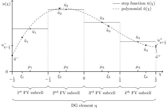
Figure 3: Schematic of four ($N=4$) mean values and the reconstructed polynomial on the reference element. The cell boundary values $u_{q-\frac{1}{2}}^{-}$ and $u_{q+\frac{1}{2}}^{+}$ were calculated with (37) where we assumed a blending factor of $\alpha=0.75$.

The fundamental issue of the naïve single-level blending discretization (35) is that it is not conservative if the blending parameter $\alpha_{q}$ varies from element to element. It turns out that the direct blending of the surface fluxes of both discretizations, namely $\bm{f}_{q}^{*(\text{FV})}$ and $\bm{f}_{q}^{*(\text{DG})}$, leads to a non-conservative balance of the net fluxes across element interfaces. To remedy this issue the goal is to define unique surface fluxes common to both, the low order and the high order discretization, such that they can be directly blended. We thus compute a blending of the reconstructed interface values to evaluate a unique common surface flux $\bm{f}_{q}^{*}$. First, we define two interface vectors of length $N+1$

$$\bm{u}_{q}^{+}:=\big{(}\underbrace{u_{q-\frac{1}{2}}^{+},(\bar{u}_{1})_{q},\ldots,(\bar{u}_{N-1})_{q},u_{q+\frac{1}{2}}^{+}}_{\begin{subarray}{c}\text{prolongated states at}\\ \text{FV subcell interfaces}\end{subarray}}\big{)}^{T}\quad\text{and}\quad\bm{u}_{q}^{-}:=\big{(}\underbrace{u_{q-\frac{1}{2}}^{-},(\bar{u}_{2})_{q},\ldots,(\bar{u}_{N})_{q},u_{q+\frac{1}{2}}^{-}}_{\begin{subarray}{c}\text{prolongated states at}\\ \text{FV subcell interfaces}\end{subarray}}\big{)}^{T},$$ (36)

where the outermost interface values are given by

$$u_{q-\frac{1}{2}}^{-}=(1-\alpha_{q})\,(\bar{u}_{1})_{q}+\alpha_{q}\,\tilde{u}_{q}^{-}\quad\text{and}\quad u_{q+\frac{1}{2}}^{+}=(1-\alpha_{q})\,(\bar{u}_{N})_{q}+\alpha_{q}\,\tilde{u}_{q}^{+}.$$ (37)

A concrete example for the blended boundary values $u_{q\pm\frac{1}{2}}^{\pm}$ is shown in Fig. 3.

The common surface flux $\bm{f}_{q}^{*}$ is then evaluated with the interface vectors $\bm{u}_{q}^{+}$ and $\bm{u}_{q}^{-}$ as

$$\bm{f}_{q}^{*}=f^{*}\left(\bm{u}_{q}^{+},\bm{u}_{q}^{-}\right)\;\in\mathbb{R}^{N+1}.$$ (38)

To make the DG surface operator $\bm{B}$ compatible with $\bm{f}_{q}^{*}$, we adapt the notation by inserting an additional column of zeros

$$\bm{B}^{(0)}=\begin{pmatrix}B_{11}&0&\cdots&0&\cdots&0&B_{1N}\\ B_{21}&0&\cdots&0&\cdots&0&B_{2N}\\ \vdots&\vdots&\ddots&\vdots&\ddots&\vdots&\vdots\\ B_{N1}&0&\cdots&0&\cdots&0&B_{NN}\\ \end{pmatrix}\;\in\mathbb{R}^{N\times(N+1)}.$$ (39)

Corollary: Contracting the DG surface operator $\bm{B}^{(0)}$ with the quadrature weights $\bm{\omega}$ is equivalent to the contraction of the FV surface operator, i.e.

$$\bm{\omega}^{T}\,\bm{B}^{(0)}=\bm{1}^{T}\,\bm{\Delta}^{(S)}.$$ (40)

Proof: We expand the left side of (40) and write

$$\bm{\omega}^{T}\,\bm{B}^{(0)} =\left(-\sum_{i=1}^{N}\omega_{i}\frac{\ell_{i}(-\tfrac{1}{2})}{\omega_{i}},0,\ldots,0,\sum_{i=1}^{N}\omega_{i}\frac{\ell_{i}(\tfrac{1}{2})}{\omega_{i}}\right)$$

$$=\left(-\sum_{i=1}^{N}\ell_{i}(-\tfrac{1}{2}),0,\ldots,0,\sum_{i=1}^{N}\ell_{i}(\tfrac{1}{2})\right)=\left(-1,0,\ldots,0,1\right)=\bm{1}^{T}\,\bm{\Delta}^{(S)}.$$

$\square$

We replace $\bm{f}_{q}^{*(\text{FV})}$ and $\bm{f}_{q}^{*(\text{DG})}$ in (35) with $\bm{f}_{q}^{*}$, and additionally, write the DG operators compactly, including the projection operator, as

$$\hat{\bm{D}}=\bm{P}\,\bm{D}\quad\text{and}\quad\hat{\bm{B}}=\bm{P}\,\bm{B}^{(0)}.$$ (41)

The final form of the single-level blended discretization is

$$\partial_{t}\bm{\bar{u}}_{q}=(1-\alpha_{q})\,\frac{-N}{\Delta x}\,\bm{\Delta}\,\bm{f}_{q}^{*}+\alpha_{q}\,\frac{1}{\Delta x}\,\left(\hat{\bm{D}}\,\bm{\tilde{f}}_{q}-\hat{\bm{B}}\,\bm{f}_{q}^{*}\right).$$ (42)

Remark: It is easy to see that with $\alpha_{q}=0$ for all elements $q$, the pure subcell FV discretization is recovered and with $\alpha_{q}=1$ for all elements the blending scheme recovers the pure high order DG method.

Lemma: Given arbitrary blending factors $\alpha_{q}\in\mathbb{R}$ for each element $q$ the blending scheme (42) is conservative.

Proof: We discretely integrate the single-level blended discretization over all elements $q$ with a total number of $Q$

$$\sum_{q}^{Q}\Delta x_{q}\,\bm{1}^{T}\partial_{t}\bm{\bar{u}}_{q}=\sum_{q}^{Q}\Delta x_{q}\,\bm{1}^{T}\Big{\{}(1-\alpha_{q})\,\frac{-N}{\Delta x_{q}}\,\bm{\Delta}\,\bm{f}^{*}_{q}+\alpha_{q}\,\frac{1}{\Delta x_{q}}\left(\hat{\bm{D}}\,\bm{\tilde{f}}_{q}-\hat{\bm{B}}\,\bm{f}^{*}_{q}\right)\Big{\}}.$$

With (9) and (41) we get

$$\sum_{q}^{Q}\Delta x_{q}\,\bm{1}^{T}\partial_{t}\bm{\bar{u}}_{q}=\sum_{q}^{Q}\bm{1}^{T}\Big{\{}-(1-\alpha_{q})\,N\,\big{(}\bm{\Delta}^{(V)}+\bm{\Delta}^{(S)}\big{)}\,\bm{f}^{*}_{q}+\alpha_{q}\,\left(\bm{P}\,\bm{D}\,\bm{\tilde{f}}_{q}-\bm{P}\,\bm{B}^{(0)}\,\bm{f}^{*}_{q}\right)\Big{\}}.$$

With properties (10), (24) and (26) the volume terms vanish, i.e.

$$\bm{1}^{T}\,\bm{\Delta}^{(V)}=\bm{0}^{T}\quad\text{and}\quad\bm{1}^{T}\,\bm{P}\,\bm{D}=N\,\bm{\omega}^{T}\,\bm{D}=\bm{0}^{T}.$$

We reformulate the DG surface term with (26) and (40) as

$$\bm{1}^{T}\,\bm{P}\,\bm{B}^{(0)}=N\,\bm{\omega}^{T}\,\bm{B}^{(0)}=N\,\bm{1}^{T}\bm{\Delta}^{(S)}.$$

The expansion of the telescopic sum only leaves the outermost surface fluxes

$$\sum_{q}^{Q}\Big{[}-(1-\alpha_{q})\,N\,\bm{1}^{T}\bm{\Delta}^{(S)}-\alpha_{q}\,N\,\bm{1}^{T}\bm{\Delta}^{(S)}\Big{]}\,\bm{f}^{*}_{q}=\sum_{q}^{Q}-N\,\bm{1}^{T}\bm{\Delta}^{(S)}\,\bm{f}^{*}_{q}\\$$

$$=-N\,\Big{(}\big{(}-f^{*}_{1}\big{)}_{1}+\big{(}f^{*}_{N+1}\big{)}_{Q}\Big{)}=0,$$

which represent the change due to physical boundary conditions. For instance in case of periodic boundary conditions, these two fluxes would cancel to zero. $\quad\square$

This concludes the description of the single-level blending scheme.

2.6 Multi-level Blending

As mentioned in the introduction, the general idea is the construction of a hierarchy of discretizations, with lower order DG schemes on sub-elements. In principle, it is thus possible to define a multi-level blending discretization, where the low order FV scheme is blended with DG variants of different approximation order. This multi-level extension is driven by the desire to retain as much ’high order DG accuracy’ as possible, especially on a sub-element level.

For the discussion, we consider a specific example setup with a DG element with polynomial degree $N_{p}=7$. The data of this DG element is collected in form of $N=8$ mean values on a regular subcell grid. Our goal is to blend a first order subcell FV scheme, a second and fourth order sub-element DG scheme and the full eight order DG scheme. The construction of the individual schemes follows the discussion in the previous sections 2.1, 2.2, and 2.5. In this section, the extension to a multi-level blending approach is presented.

We get the first data interpretation and its corresponding discretization by directly using the mean values of element $q$ as a first order approximation space with no reconstruction at all

$$\bm{\bar{u}}_{q}^{\mathcal{O}(1)}:=\bm{\bar{u}}_{q}=(\bar{u}_{1},\bar{u}_{2},\ldots,\bar{u}_{8})_{q}^{T}.$$

Next, we interpret the eight mean values as four second order DG sub-elements. The reconstruction matrix $\bm{R}^{\mathcal{O}(2)}\in\mathbb{R}^{2\times 2}$ transforms two adjacent mean values to two nodal values

$$\bm{\tilde{u}}_{q}^{\mathcal{O}(2)}=\Big{(}\underbrace{\left(\tilde{u}_{1}\right)_{1}^{\mathcal{O}(2)},\left(\tilde{u}_{2}\right)_{1}^{\mathcal{O}(2)}}_{\mathcal{O}(2)-\text{sub-element}},\ldots,\underbrace{\left(\tilde{u}_{1}\right)_{4}^{\mathcal{O}(2)},\left(\tilde{u}_{2}\right)_{4}^{\mathcal{O}(2)}}_{\mathcal{O}(2)-\text{sub-element}}\Big{)}_{q}^{T}=\left[\bm{\mathds{1}}_{4}\otimes\bm{R}^{\mathcal{O}(2)}\right]\,\bm{\bar{u}}_{q}.$$ (43)

The fourth and eight order approximations are constructed analogously as

$$\bm{\tilde{u}}_{q}^{\mathcal{O}(4)}=\Big{(}\underbrace{\left(\tilde{u}_{1}\right)_{1}^{\mathcal{O}(4)},\ldots,\left(\tilde{u}_{4}\right)_{1}^{\mathcal{O}(4)}}_{\mathcal{O}(4)-\text{sub-element}},\underbrace{\left(\tilde{u}_{1}\right)_{2}^{\mathcal{O}(4)},\ldots,\left(\tilde{u}_{4}\right)_{2}^{\mathcal{O}(4)}}_{\mathcal{O}(4)-\text{sub-element}}\Big{)}_{q}^{T}=\left[\bm{\mathds{1}}_{2}\otimes\bm{R}^{\mathcal{O}(4)}\right]\,\bm{\bar{u}}_{q},$$ (44)

and

$$\bm{\tilde{u}}_{q}^{\mathcal{O}(8)}=\Big{(}\underbrace{\tilde{u}_{1}^{\mathcal{O}(8)},\ldots,\tilde{u}_{8}^{\mathcal{O}(8)}}_{\mathcal{O}(8)-\text{sub-element}}\Big{)}_{q}^{T}=\left[\bm{\mathds{1}}_{1}\otimes\bm{R}^{\mathcal{O}(8)}\right]\,\bm{\bar{u}}_{q},$$ (45)

with $\bm{R}^{\mathcal{O}(4)}\in\mathbb{R}^{4\times 4}$ and $\bm{R}^{\mathcal{O}(8)}\in\mathbb{R}^{8\times 8}$. Here we used the Kronecker product $\otimes$ in conjunction with the identity matrix $\bm{\mathds{1}}_{n}=\text{diag}(1,\ldots,1)\in\mathbb{R}^{n\times n}$ in order to generate appropriate block-diagonal matrices. Fig. 18 in appendix 6.1 illustrates the hierarchy of the approximation spaces for this example.

We correspond the approximation spaces with the respective discretizations

$$\partial_{t}\bm{\bar{u}}_{q}^{\mathcal{O}(1)} =-\frac{8}{\Delta x_{q}}\;\bm{\Delta}\,\bm{f}^{*}$$

$$\partial_{t}\bm{\bar{u}}_{q}^{\mathcal{O}(2)} =\,\;\;\frac{4}{\Delta x_{q}}\left\{\left[\bm{\mathds{1}}_{4}\otimes\hat{\bm{D}}^{\mathcal{O}(2)}\right]\bm{\tilde{f}}_{q}^{\mathcal{O}(2)}-\left[\bm{\mathds{1}}_{4}\otimes\hat{\bm{B}}^{\mathcal{O}(2)}\right]^{(0)}\bm{f}_{q}^{*}\right\},$$

$$\partial_{t}\bm{\bar{u}}_{q}^{\mathcal{O}(4)} =\,\;\;\frac{2}{\Delta x_{q}}\left\{\left[\bm{\mathds{1}}_{2}\otimes\hat{\bm{D}}^{\mathcal{O}(4)}\right]\bm{\tilde{f}}_{q}^{\mathcal{O}(4)}-\left[\bm{\mathds{1}}_{2}\otimes\hat{\bm{B}}^{\mathcal{O}(4)}\right]^{(0)}\bm{f}_{q}^{*}\right\},$$ (46)

$$\partial_{t}\bm{\bar{u}}_{q}^{\mathcal{O}(8)} =\,\;\;\frac{1}{\Delta x_{q}}\left\{\left[\bm{\mathds{1}}_{1}\otimes\hat{\bm{D}}^{\mathcal{O}(8)}\right]\bm{\tilde{f}}_{q}^{\mathcal{O}(8)}-\left[\bm{\mathds{1}}_{1}\otimes\hat{\bm{B}}^{\mathcal{O}(8)}\right]^{(0)}\bm{f}_{q}^{*}\right\},$$

where the DG volume fluxes are computed with the respective polynomial (sub-)element reconstructions of orders $n=\{2,4,8\}$:

$$\bm{\tilde{f}}_{q}^{\mathcal{O}(n)}=f\left(\bm{\tilde{u}}_{q}^{\mathcal{O}(n)}\right).$$

Similar to (39) the DG surface operators $\big{[}\bm{\mathds{1}}_{N/n}\otimes\hat{\bm{B}}^{\mathcal{O}(n)}\big{]}$ had to be slightly adapted in order to be compatible with the common surface flux $\bm{f}^{*}$. We list the modified boundary evaluation matrices in the appendix 6.2. Finally, all four candidate discretizations are blended starting from the lowest order up to the highest order discretization

$$\partial_{t}\bm{\bar{u}}_{q}^{{}^{\prime\prime\prime}} :=\partial_{t}\bm{\bar{u}}_{q}^{\mathcal{O}(1)},$$

$$\hookrightarrow\;\partial_{t}\bm{\bar{u}}_{q}^{{}^{\prime\prime}} =\left(\bm{1}-\bm{\alpha}_{q}^{\mathcal{O}(2)}\right)\odot\partial_{t}\bm{\bar{u}}_{q}^{{}^{\prime\prime\prime}}+\bm{\alpha}_{q}^{\mathcal{O}(2)}\odot\partial_{t}\bm{\bar{u}}_{q}^{\mathcal{O}(2)},$$

$$\hookrightarrow\;\partial_{t}\bm{\bar{u}}_{q}^{{}^{\prime}} =\left(\bm{1}-\bm{\alpha}_{q}^{\mathcal{O}(4)}\right)\odot\partial_{t}\bm{\bar{u}}_{q}^{{}^{\prime\prime}}+\bm{\alpha}_{q}^{\mathcal{O}(4)}\odot\partial_{t}\bm{\bar{u}}_{q}^{\mathcal{O}(4)},$$ (47)

$$\hookrightarrow\;\partial_{t}\bm{\bar{u}}_{q} =\left(\bm{1}-\bm{\alpha}_{q}^{\mathcal{O}(8)}\right)\odot\partial_{t}\bm{\bar{u}}_{q}^{{}^{\prime}}+\bm{\alpha}_{q}^{\mathcal{O}(8)}\odot\partial_{t}\bm{\bar{u}}_{q}^{\mathcal{O}(8)},$$

where $\odot$ denotes the component-wise multiplication with the vector of blending parameters. Each DG sub-element computes its own blending factor according to the local data, i.e. we get 4 blending factors for the $\mathcal{O}(2)$ variant, 2 blending factors for $\mathcal{O}(4)$ and 1 for $\mathcal{O}(8)$
$\bm{\alpha}_{q}^{\mathcal{O}(2)}=$ $\left(\alpha_{1}^{\mathcal{O}(2)},\alpha_{2}^{\mathcal{O}(2)},\alpha_{3}^{\mathcal{O}(2)},\alpha_{4}^{\mathcal{O}(2)}\right)_{q}^{T}$ $\otimes$ $(1,1)^{T}$, $\bm{\alpha}_{q}^{\mathcal{O}(4)}=$ $\left(\alpha_{1}^{\mathcal{O}(4)},\alpha_{2}^{\mathcal{O}(4)}\right)_{q}^{T}$ $\otimes$ $(1,1,1,1)^{T}$, $\bm{\alpha}_{q}^{\mathcal{O}(8)}=$ $\left(\alpha^{\mathcal{O}(8)}\right)_{q}^{T}$ $\otimes$ $(1,1,1,1,1,1,1,1)^{T}$.
The actual strategy for the blending factors is described in the next section 2.7.

Again, as discussed in the case of a single-blending approach in section 2.5, special care is needed to preserve the conservation of the final discretization. Expanding on the idea in the single-level case, we aim to compute unique surface fluxes for each discretization with a uniquely defined interface value at sub-element or subcell interfaces. We evaluate all high order DG polynomials at the FV subcell interfaces $\bm{u}_{q}^{\pm\mathcal{O}(n)}\in\mathbb{R}^{N}$

$$\bm{u}_{q}^{\pm\mathcal{O}(1)} :=\bm{\bar{u}}_{q}^{\mathcal{O}(1)}, \bm{u}_{q}^{\pm\mathcal{O}(2)} =\left[\bm{\mathds{1}}_{4}\otimes\bm{I}^{\pm\mathcal{O}(2)}\right]\,\bm{\tilde{u}}_{q}^{\mathcal{O}(2)},$$

$$\bm{u}_{q}^{\pm\mathcal{O}(4)} =\left[\bm{\mathds{1}}_{2}\otimes\bm{I}^{\pm\mathcal{O}(4)}\right]\,\bm{\tilde{u}}_{q}^{\mathcal{O}(4)}, \bm{u}_{q}^{\pm\mathcal{O}(8)} =\left[\bm{\mathds{1}}_{1}\otimes\bm{I}^{\pm\mathcal{O}(8)}\right]\,\bm{\tilde{u}}_{q}^{\mathcal{O}(8)},$$

where the interpolation operator $\bm{I}^{\pm\mathcal{O}(n)}\in\mathbb{R}^{n\times n}$ prolongates to the embedded FV subcell interfaces $\mu^{\mathcal{O}(n)}_{i\pm 1/2}$ of the respective DG sub-element, i.e.

$$\left(\bm{I}^{\pm\mathcal{O}(n)}\right)_{ij}=\ell^{\mathcal{O}(n)}_{j}\left(\mu^{\mathcal{O}(n)}_{i\pm 1/2}\right),\quad i,j=1,\ldots,n.$$ (48)

In Fig. 18 in appendix 6.1 two representatives of $\mu^{\mathcal{O}(n)}_{i\pm 1/2}$ are shown which are aligned at the dotted vertical lines, indicating the interfaces of the FV subcells.

We start with the first order interpolation and stack on top the next levels of orders via convex blending

$$\left(\bm{u}_{q}^{\pm}\right)^{{}^{\prime\prime\prime\prime}} :=\bm{u}_{q}^{\pm\mathcal{O}(1)}$$

$$\hookrightarrow\;\left(\bm{u}_{q}^{\pm}\right)^{{}^{\prime\prime\prime}} =\left[\bm{1}-\bm{\alpha}_{q}^{\mathcal{O}(2)}\right]\odot\left(\bm{u}_{q}^{\pm}\right)^{{}^{\prime\prime\prime\prime}}+\bm{\alpha}_{q}^{\mathcal{O}(2)}\odot\bm{u}_{q}^{\pm\mathcal{O}(2)}$$

$$\hookrightarrow\>\left(\bm{u}_{q}^{\pm}\right)^{{}^{\prime\prime}} =\left[\bm{1}-\bm{\alpha}_{q}^{\mathcal{O}(4)}\right]\odot\left(\bm{u}_{q}^{\pm}\right)^{{}^{\prime\prime\prime}}+\bm{\alpha}_{q}^{\mathcal{O}(4)}\odot\bm{u}_{q}^{\pm\mathcal{O}(4)}$$

$$\hookrightarrow\>\left(\bm{u}_{q}^{\pm}\right)^{{}^{\prime}} =\left[\bm{1}-\bm{\alpha}_{q}^{\mathcal{O}(8)}\right]\odot\left(\bm{u}_{q}^{\pm}\right)^{{}^{\prime\prime}}+\bm{\alpha}_{q}^{\mathcal{O}(8)}\odot\bm{u}_{q}^{\pm\mathcal{O}(8)}.$$

To arrive at a complete vector of interface values we append the element interface values from the left and right neighbors $q-1$ and $q+1$.

$$\bm{u}_{q}^{+} =\Big{(}\overbrace{\left(u^{+}_{N}\right)_{q-1}^{{}^{\prime}},}^{\text{left neighbor}}\quad\overbrace{\left(u^{+}_{1},\ldots,u^{+}_{N}\right)_{q}^{{}^{\prime}}}^{\text{internal boundaries}}\Big{)}^{T},$$

$$\bm{u}_{q}^{-} =\Big{(}\underbrace{\left(u^{-}_{1},\ldots,u^{-}_{N}\right)_{q}^{{}^{\prime}},}_{\text{internal boundaries}}\quad\underbrace{\left(u^{-}_{1}\right)_{q+1}^{{}^{\prime}}}_{\text{right neighbor}}\Big{)}^{T}.$$

These new common interface values allow us to evaluate a common surface flux (38) at each interface, which is again the key to preserve conservation in the final discretization. This concludes the description of the multi-level blending scheme.

2.7 Calculation of the Blending Factor $\alpha$

A good shock indicator for high order methods is supposed to recognize discontinuities, such as weak and strong shocks, in the solution early on and mark the affected elements for proper shock capturing. On the other hand, the indicator should avoid to flag non-shock related fluid features such as shear layers and turbulent flows. There are numerous indicators available for DG schemes [50, 15, 14, 60, 2, 9, 66].

In this work we want to construct an a-priori indicator which relies on the readily available information within each element provided by the multi-level blending framework introduced in section 2.6. The principal idea is to compare a measure of smoothness of the different order reconstructions with each other. Smooth, well-resolved flows are expected to yield rather similar solution profiles compared to data that contain strong variations.

The smoothness measure $\sigma_{q}^{\mathcal{O}(n)}$ within element $q$ of the $n$-th order reconstruction $\tilde{u}_{q}^{\mathcal{O}(n)}$ is inferred from the $L^{1}$-norm of its first derivative. For example, if we want to calculate the blending factor $\alpha_{q}^{\mathcal{O}(8)}$ for the eighth order we compute

$$\sigma_{q}^{\mathcal{O}(8)}=\int_{-\frac{1}{2}}^{\frac{1}{2}}\left|\partial_{\xi}\tilde{u}_{q}^{\mathcal{O}(8)}(\xi)\right|d\xi$$ (49)

and

$$\sigma_{q}^{\mathcal{O}(4)}=\left(\sigma_{1}^{\mathcal{O}(4)}\right)_{q}+\left(\sigma_{2}^{\mathcal{O}(4)}\right)_{q}=\int_{-\frac{1}{2}}^{0}\left|\partial_{\xi}\left(\tilde{u}_{1}^{\mathcal{O}(4)}\right)_{q}(\xi)\right|d\xi+\int_{0}^{\frac{1}{2}}\left|\partial_{\xi}\left(\tilde{u}_{2}^{\mathcal{O}(4)}\right)_{q}(\xi)\right|d\xi$$

utilizing information from the top-level eighth order element and its two fourth order sub-elements. The integrals are evaluated with appropriate quadrature rules. Then the blending factor is calculated by comparing the smoothness of the different orders as

$$\alpha_{q}^{\mathcal{O}(8)}=1-\text{cutoff}\left(0,\tau_{A}\,\left(\frac{\left|\sigma_{q}^{\mathcal{O}(8)}-\sigma_{q}^{\mathcal{O}(4)}\right|}{\max\big{(}\sigma_{q}^{\mathcal{O}(4)},\sigma_{q}^{\mathcal{O}(8)},1\big{)}}-\tau_{S}\right),1\right),$$ (50)

where $\text{cutoff}(x_{\text{lower}},x,x_{\text{upper}})=\min(\max(x_{\text{lower}},x),x_{\text{upper}})$ and with two parameters $\tau_{A},\tau_{S}>0.$ The design of equation (50) ensures that $\alpha_{q}^{\mathcal{O}(n)}$ is always within the unit interval and that for very small $\sigma_{q}^{\mathcal{O}(n)}$ the indicator does not get hypersensitive due to floating point truncation. If not noted otherwise we set the amplification parameter to $\tau_{A}=100$ and the sensitivity parameter $\tau_{S}=0.05$. The latter parameter has the biggest influence on the behavior of the indicator and its value demarcates the lower bound where it does not interfere with the convergence tests conducted in section 3. In order to capture all troubling flow features we independently apply the indicator (50) on all primitive state variables and select the smallest of the resulting blending factors. The calculations of the two fourth order blending factors $\left(\alpha_{1}^{\mathcal{O}(4)}\right)_{q}$ and $\left(\alpha_{2}^{\mathcal{O}(4)}\right)_{q}$ are done within each sub-element independently together with their respective second order smoothness measures $\left(\sigma_{s}^{\mathcal{O}(2)}\right)_{q}$, $s=1,\ldots,4$.

For piecewise linear polynomials, the indicator (50) is not applicable. Instead, we directly use the squeezing parameter $\beta$ obtained from the positivity limiter in (30), i.e. $\alpha_{s}^{\mathcal{O}(2)}:=\beta_{s}^{\mathcal{O}(2)}$, $s=1,\ldots,4$.

Remark: The indicator (50) is also used for the single-level blending scheme.

2.8 Sketch of the Algorithm

In the last part of this section, a sketch of the algorithm for the blending framework is presented. We present a general outline of the necessary steps for the 1D single-blending scheme evolved with a multi-stage Runge-Kutta time stepping method. We enter at the beginning of a Runge-Kutta cycle and do the following.

1. Reconstruct the polynomial $\bm{\tilde{u}}_{q}$ from the given mean values $\bm{\bar{u}}_{q}$ for each element $q$ as in (28).

2. If the reconstructed polynomial $\bm{\tilde{u}}_{q}$ contains non-permissible states, see (31), then calculate the limited version $\bm{\tilde{u}}_{q}^{(\beta)}$ as in (30)

3. If the squeezing parameter $\beta_{q}$ is below $\beta_{L}$ then set $\alpha_{q}:=0$ else compute the blending factor $\alpha_{q}$ via (50) from the unlimited polynomial $\bm{\tilde{u}}_{q}$.

4. Compute the boundary values $u_{q}^{\pm}$ via (37) and exchange alongside zone boundaries in case of distributed computing.

5. Determine the common surface flux $\bm{f}_{q}^{*}$ via (38).

6. Calculate the right-hand-side $\partial_{t}\bm{\bar{u}}_{q}$:

   • If the blending factor $\alpha_{q}$ above $\alpha_{H}$ then compute $\partial_{t}\bm{\bar{u}}_{q}$ with the DG-only scheme.

   • Else if the blending factor $\alpha_{q}$ below $\alpha_{L}$ then compute $\partial_{t}\bm{\bar{u}}_{q}$ with the FV-only scheme.

   • Else compute $\partial_{t}\bm{\bar{u}}_{q}$ with the single-level blending scheme (42).

7. Forward in time to the next Runge-Kutta stage and return to step (I).

The switching thresholds are set to $\alpha_{H}:=0.99$ and $\alpha_{L}:=0.01$ and the limiter threshold to $\beta_{L}:=0.95$. Note that the algorithm only applies the blending procedure where necessary in order to maintain the overall performance of the scheme.

This concludes the presentation of the 1D blending scheme. The description of the blending scheme on 3D Cartesian meshes as well as the algorithm outline for the multi-level blending scheme can be found in appendix 6.3 and 6.4.

3 Validation

For the computational investigations, the multi-level algorithm with the explicit SSP-RK(5,4) time integrator [59] is implemented in a Fortran-2008 prototype code with a hybrid parallelization strategy based on MPI and OpenMP. Management of the AMR and load balancing is provided by p4est, a highly efficient Octree library [4]. The maximal time step for dimensions $d=1,2,3$ is estimated by the CFL condition

$$\Delta t:=CFL\,\min_{q}\;\frac{\Delta x_{q}}{2^{d-1}(2\,N-1)\,\bar{\lambda}_{q,\text{max}}},$$ (51)

where $CFL:=0.8$, $N:=8$ is the number of mean values in each direction of the element $q$ and $\bar{\lambda}_{q,\text{max}}$ is an estimate of the maximum eigenvalue given in (55). For the numerical interface fluxes $f^{*}$, we use the Harten-Lax-Leer (HLL) approximate Riemann solver [29] with Einfeldt signal speed estimates [16].

3.1 Governing Equations

We consider the compressible Euler equations

$$\partial_{t}\rho+\nabla\cdot(\rho\,\bm{v}) =0,$$

$$\partial_{t}(\rho\,\bm{v})+\nabla\cdot\left(\rho\,\bm{v}\bm{v}^{T}+p\,\bm{\mathds{1}}\right) =\bm{0},$$ (52)

$$\partial_{t}\mathcal{E}+\nabla\cdot\Big{(}\bm{v}\,(\mathcal{E}+p)\Big{)} =0,$$

with the vector of conserved quantities $\bm{u}=(\rho,\rho\,\bm{v},\mathcal{E})^{T}$, where $\rho$ denotes the density, $\bm{v}$ the velocity, and $\mathcal{E}$ the total energy. We assume a perfect gas equation of state and compute the pressure as

$$p(\bm{u})=(\gamma-1)\,\left[\mathcal{E}-\frac{\rho}{2}\,\bm{v}^{T}\bm{v}\right].$$ (53)

If not stated otherwise we choose $\gamma=1.4$. The set of permissible states is given by

$$\big{\{}\text{permissible states}\big{\}}=\big{\{}\forall\,\bm{u}\;\big{|}\;\rho>0\wedge p(\bm{u})>0\big{\}}.$$ (54)

For the CFL condition (51) the maximum eigenvalue is evaluated on all mean values $\bm{\bar{u}}_{q}$ of element $q$. Given dimension $d=\{1,2,3\}$ it reads as

$$\bar{\lambda}_{q,\text{max}}=\max_{i,d}\left(\big{|}(\bar{v}_{d})_{i}\big{|}+\sqrt{\gamma\,\frac{\bar{p}_{i}}{\bar{\rho}_{i}}}\right),\quad i=1,\ldots,N^{d_{\text{max}}}.$$ (55)

3.2 Convergence Test

We use the manufactured solution method [52] and validate the 3D multi-level blending scheme on a periodic cube of unit length ($L=1$) where the resolution of the mesh is incrementally doubled. We define our manufactured solution in primitive state variables as

$$\rho(t;x,y,z) =1.0+0.35\,\sin\left(\frac{2\,\pi\,(x-t)}{L}\right)+0.24\,\cos\left(\frac{2\,\pi\,(y-t)}{L}\right)+0.1\,\sin\left(\frac{2\,\pi\,(z-t)}{L}\right),$$

$$\bm{v}(t;x,y,z) =(0.1,0.2,0.3)^{T},$$ (56)

$$p(t;x,y,z) =1.0+0.23\,\cos\left(\frac{2\,\pi\,(x-t)}{L}\right)+0.19\,\sin\left(\frac{2\,\pi\,(y-t)}{L}\right)+0.2\,\cos\left(\frac{2\,\pi\,(z-t)}{L}\right).$$

The final time of the simulation is $T=2$ and the center of the domain is refined to introduce non-conforming interfaces in the computational domain. We determine the $L^{\infty}$- and $L^{2}$-norms of the errors in the density and total energy. Tables 1 to 4 list the results for the first, second, fourth and eighth order multi-level blending schemes. The initial conditions and the source term of our manufactured solution (3.2) is in all cases evaluated and applied on the mean values via an appropriate quadrature rule to maintain high order. The results confirm, that the discretizations behave as designed in this assessment.

Table 1: Experimental order of convergence of the first-order FV variant within the 3D multi-level blending framework.

resol.	density		total energy		density		total energy
$2^{r}$	$||\epsilon||_{\infty}$	$||\epsilon||_{2}$	$||\epsilon||_{\infty}$	$||\epsilon||_{2}$	$EOC_{\infty}$	$EOC_{2}$	$EOC_{\infty}$	$EOC_{2}$
16	5.98e-03	4.84e-03	1.34e-02	1.03e-02	n/a	n/a	n/a	n/a
32	3.51e-03	2.83e-03	7.91e-03	6.13e-03	0.77	0.77	0.76	0.75
64	2.21e-03	1.45e-03	4.30e-03	3.13e-03	0.67	0.97	0.88	0.97
128	1.42e-03	7.30e-04	2.26e-03	1.57e-03	0.63	0.99	0.93	0.99

Table 2: Experimental order of convergence of the second order DG variant within the 3D multi-level blending framework.

resol.	density		total energy		density		total energy
$2^{r}$	$||\epsilon||_{\infty}$	$||\epsilon||_{2}$	$||\epsilon||_{\infty}$	$||\epsilon||_{2}$	$EOC_{\infty}$	$EOC_{2}$	$EOC_{\infty}$	$EOC_{2}$
16	1.46e-03	5.38e-04	2.21e-03	9.35e-04	n/a	n/a	n/a	n/a
32	4.59e-04	9.29e-05	6.63e-04	1.97e-04	1.67	2.53	1.74	2.25
64	1.11e-04	1.77e-05	1.48e-04	4.26e-05	2.04	2.39	2.17	2.21
128	2.63e-05	3.88e-06	3.09e-05	9.72e-06	2.08	2.19	2.25	2.13

Table 3: Experimental order of convergence of the fourth order DG variant within the 3D multi-level blending framework.

resol.	density		total energy		density		total energy
$2^{r}$	$||\epsilon||_{\infty}$	$||\epsilon||_{2}$	$||\epsilon||_{\infty}$	$||\epsilon||_{2}$	$EOC_{\infty}$	$EOC_{2}$	$EOC_{\infty}$	$EOC_{2}$
16	1.10e-04	6.45e-05	3.20e-04	1.83e-04	n/a	n/a	n/a	n/a
32	7.86e-06	4.33e-06	2.19e-05	1.33e-05	3.80	3.90	3.87	3.79
64	5.18e-07	2.59e-07	1.31e-06	7.59e-07	3.92	4.07	4.07	4.13
128	3.45e-08	1.82e-08	7.75e-08	4.29e-08	3.91	3.83	4.07	4.15

Table 4: Experimental order of convergence of the eighth order DG variant within the 3D multi-level blending framework. Here we set $CFL:=0.1$, as the time integration method is only fourth order accurate.

resol.	density		total energy		density		total energy
$2^{r}$	$||\epsilon||_{\infty}$	$||\epsilon||_{2}$	$||\epsilon||_{\infty}$	$||\epsilon||_{2}$	$EOC_{\infty}$	$EOC_{2}$	$EOC_{\infty}$	$EOC_{2}$
16	2.77e-07	1.65e-07	7.77e-07	4.55e-07	n/a	n/a	n/a	n/a
32	2.77e-09	1.00e-09	6.72e-09	2.41e-09	6.65	7.36	6.85	7.56
64	1.73e-11	3.48e-12	4.15e-11	1.04e-11	7.32	8.17	7.34	7.86
128	8.06e-14	1.87e-14	1.85e-13	6.74e-14	7.74	7.54	7.81	7.27

3.3 Conservation Test

The goal in this assessment is to demonstrate that the multi-level-blending discretization is conservative for all choices of blending factors. To do so, we adapt the same setup as in section 3.2 but deactivate the source term. The center of the domain is refined to introduce non-conforming interfaces in the computational domain. Additionally, as a stress test, the blending factors are randomly chosen and changed after each Runge-Kutta stage. As there are multiple blending factors at a given spatial location, we consider the following weighted blending factor

$$\bar{\alpha}=\left\{\left[\left(1-\alpha^{\mathcal{O}(2)}\right)+2\,\alpha^{\mathcal{O}(2)}\right]\,\left(1-\alpha^{\mathcal{O}(4)}\right)+4\,\alpha^{\mathcal{O}(4)}\right\}\,\left(1-\alpha^{\mathcal{O}(8)}\right)+8\,\alpha^{\mathcal{O}(8)},$$ (57)

to illustrate the distribution of the blending factors in Fig.4. Note the limiting cases $\bar{\alpha}=1$ for pure FV and $\bar{\alpha}=8$ for the eighth order DG scheme.

The simulation runs to $T=300$ performing more than a quarter million timesteps. The result of the test is shown in Fig. 5 where we plot in log-scale the absolute value of the change of bulk $\partial_{t}\mathbf{\bar{u}}_{\text{total}}(t)$, integrated over the whole domain,

$$\partial_{t}\mathbf{\bar{u}}_{\text{total}}(t)=\sum_{q}^{Q}\frac{1}{|\Omega_{q}|}\int_{\Omega_{q}}\partial_{t}\mathbf{\bar{u}}(t)\,d\Omega.$$ (58)

$Q$ is the total number of elements and $|\Omega_{q}|=\Delta x_{q}\Delta y_{q}\Delta z_{q}$ is the volume per element. The results show that the conservation error lies within the range of 64 bit (double precision) floating point truncation and hence confirm that the multi-level blending discretization is fully conservative up to machine precision errors.

Figure 4: Conservation test of the 3D multi-level blending scheme: Slice through the computational domain showing weighted blending factor $\bar{\alpha}$ according to (57) on a Cartesian non-conforming mesh with refinement levels 3 to 5. The black lines depict the boundaries of the corresponding 8th order DG elements.

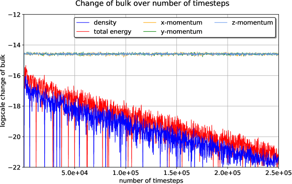
Figure 5: Conservation test of the 3D multi-level blending scheme: Evolution of the integrated change of bulk $\log_{10}(|\partial_{t}\mathbf{\bar{u}}_{\text{total}}|)$ (eq. (58)) of each conservative state variable.

3.4 1D Shock Tube Problems

We validate the multi-level blending scheme with three well-established 1D problems, namely Sod, Lax and Shu-Osher shock tubes. But first, in order to gain insights into the individual contributions of the different schemes, we introduce a more intuitive reformulation of the blending factors $\alpha^{\mathcal{O}(n)}$. The multi-level blending operation (2.6) within element $q$ can be interpreted as a linear superposition of four numerical schemes. For that, we collapse the following relations

$$\partial_{t}\bm{\bar{u}}_{q}^{{}^{\prime\prime\prime}} :=\partial_{t}\bm{\bar{u}}_{q}^{\mathcal{O}(1)},$$

$$\hookrightarrow\;\partial_{t}\bm{\bar{u}}_{q}^{{}^{\prime\prime}} =\left(\bm{1}-\bm{\alpha}_{q}^{\mathcal{O}(2)}\right)\odot\partial_{t}\bm{\bar{u}}_{q}^{{}^{\prime\prime\prime}}+\bm{\alpha}_{q}^{\mathcal{O}(2)}\odot\partial_{t}\bm{\bar{u}}_{q}^{\mathcal{O}(2)},$$

$$\hookrightarrow\;\partial_{t}\bm{\bar{u}}_{q}^{{}^{\prime}} =\left(\bm{1}-\bm{\alpha}_{q}^{\mathcal{O}(4)}\right)\odot\partial_{t}\bm{\bar{u}}_{q}^{{}^{\prime\prime}}+\bm{\alpha}_{q}^{\mathcal{O}(4)}\odot\partial_{t}\bm{\bar{u}}_{q}^{\mathcal{O}(4)},$$

$$\hookrightarrow\;\partial_{t}\bm{\bar{u}}_{q} =\left(\bm{1}-\bm{\alpha}_{q}^{\mathcal{O}(8)}\right)\odot\partial_{t}\bm{\bar{u}}_{q}^{{}^{\prime}}+\bm{\alpha}_{q}^{\mathcal{O}(8)}\odot\partial_{t}\bm{\bar{u}}_{q}^{\mathcal{O}(8)},$$

into one single term and define blending weights $\theta^{\mathcal{O}(n)}$, i.e.

$$\partial_{t}\bm{\bar{u}}_{q}=\bm{\theta}_{q}^{\mathcal{O}(1)}\odot\partial_{t}\bm{\bar{u}}_{q}^{\mathcal{O}(1)}+\bm{\theta}_{q}^{\mathcal{O}(2)}\odot\partial_{t}\bm{\bar{u}}_{q}^{\mathcal{O}(2)}+\bm{\theta}_{q}^{\mathcal{O}(4)}\odot\partial_{t}\bm{\bar{u}}_{q}^{\mathcal{O}(4)}+\bm{\theta}_{q}^{\mathcal{O}(8)}\odot\partial_{t}\bm{\bar{u}}_{q}^{\mathcal{O}(8)},$$

where

$$\bm{\theta}_{q}^{\mathcal{O}(1)} :=\left(\bm{1}-\bm{\alpha}_{q}^{\mathcal{O}(8)}\right)\odot\left(\bm{1}-\bm{\alpha}_{q}^{\mathcal{O}(4)}\right)\odot\left(\bm{1}-\bm{\alpha}_{q}^{\mathcal{O}(2)}\right),$$

$$\bm{\theta}_{q}^{\mathcal{O}(2)} :=\left(\bm{1}-\bm{\alpha}_{q}^{\mathcal{O}(8)}\right)\odot\left(\bm{1}-\bm{\alpha}_{q}^{\mathcal{O}(4)}\right)\odot\bm{\alpha}_{q}^{\mathcal{O}(2)},$$

$$\bm{\theta}_{q}^{\mathcal{O}(4)} :=\left(\bm{1}-\bm{\alpha}_{q}^{\mathcal{O}(8)}\right)\odot\bm{\alpha}_{q}^{\mathcal{O}(4)},$$ (59)

$$\bm{\theta}_{q}^{\mathcal{O}(8)} :=\bm{\alpha}_{q}^{\mathcal{O}(8)}.$$

By construction the blending weights have the following property

$$\bm{\theta}_{q}^{\mathcal{O}(1)}+\bm{\theta}_{q}^{\mathcal{O}(2)}+\bm{\theta}_{q}^{\mathcal{O}(4)}+\bm{\theta}_{q}^{\mathcal{O}(8)}=\bm{1},$$ (60)

and thus give a proper fraction of each contribution.

The first shock tube problem is the Sod shock tube [56]. It is defined on the unit interval $\Omega=[0,1]$ with a diaphragm located at $x_{D}=0.5$. The initial condition in primitive state variables reads

$$\big{(}\rho_{0}(x),v_{0}(x),p_{0}(x)\big{)}=\left\{\;\begin{aligned} \big{(}1,0,1\big{)},\quad x<x_{D},\\ \big{(}0.125,0,0.1\big{)},\quad x\geq x_{D}.\end{aligned}\right.$$

The resolution is set to 32 elements of $N=8$ mean values each. This amounts to 256 total DOF. The result for the density profile (top row) at the final simulation time $T=0.2$ is presented in Fig. 6 together with the exact solution. It shows the correct approximation of the rarefaction wave, contact discontinuity and the forward facing shock front. As designed, only at the shock front the blending scheme gets triggered, which is visible in the bottom row of the plot. The stacked bar chart directly corresponds to the blending weights $\theta^{\mathcal{O}(n)}$ in (3.4). The vertical dimension of the stacked bars completely fill the unit interval mirroring property (60).

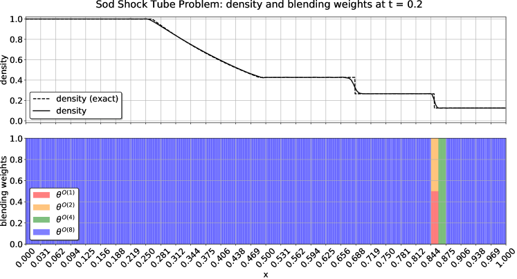
Figure 6: Sod Shock Tube Problem: Numerical solution of the density profile (top row) with the DGFV8 multi-level blending scheme together with the exact solution at final simulation time $T=0.2$. The bottom row shows the blending weights $\theta^{\mathcal{O}(n)}$ (eq. (3.4)) encoded by stacked bars in different colors. The light grey vertical grid lines depict the element boundaries.

The second test case is the Lax shock tube [42] with initial data set to

$$\big{(}\rho_{0}(x),v_{0}(x),p_{0}(x)\big{)}=\left\{\;\begin{aligned} \big{(}0.445,0.689,3.528\big{)},\quad x<x_{D},\\ \big{(}0.5,0,0.571\big{)},\quad x\geq x_{D}.\end{aligned}\right.$$

All other simulation parameters as well as the resolution are the same as in the Sod test case. The result for the density profile (top row) at final simulation time $T=0.15$ is presented in Fig. 7 together with reference solution on a finer grid of 1024 DOF with the third-order piece-wise parabolic method (PPM) [12] implemented in the astrophysics code FLASH (version 4.6, March 2019), see e.g. [21]. For comparison, we also included the solution of the PPM with the same grid resolution of 256 DOF. All flow features are resolved correctly and the blending scheme is only triggered in the region around the forward facing shock. Furthermore, this example clearly reveals the adaptive blending on the sub-element level.

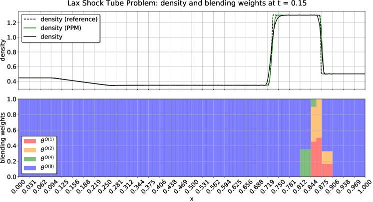
Figure 7: Lax Shock Tube Problem: Numerical solution of the density profile (top row) with the DGFV8 (256 DOF) multi-level blending scheme together with the reference solution (PPM, 1024 DOF) and PPM (256 DOF) at final simulation time $T=0.2$. The bottom row shows the blending weights $\theta^{\mathcal{O}(n)}$ (eq. (3.4)) encoded by stacked bars in different colors. The vertical grid lines depict the element boundaries.

The third shock tube, the Shu-Osher test [55], is a Mach $3$ shock interacting with a sinusoidal density wave. It reveals the scheme’s capability of capturing both, discontinuous and smooth parts of the flow. The computational domain in 1D is set to $\Omega=[-4.5,4.5]$, the final simulation time is $T=1.8$, and the primitive variables are initialized as

$$\big{(}\rho_{0}(x),v_{0}(x),p_{0}(x)\big{)}=\left\{\;\begin{aligned} \big{(}3.8567143,2.629369,10.33333\big{)},\quad x<-4,\\ \big{(}1+0.2\,\sin(5\,x),0,1\big{)},\quad x\geq-4.\end{aligned}\right.$$

Here, we compare the results of the multi-level blending DGFV8 to PPM. In order to investigate the importance of the multi-level approach on the accuracy of the DGFV8 result, we additionally perform a simulation where we intentionally deactivate the sub-elements, i.e. $\bm{\alpha}^{\mathcal{O}(2)}:=0$ and $\bm{\alpha}^{\mathcal{O}(4)}:=0$. This is identical to the single-level blending approach presented in section 2.5, where only the first order FV scheme is blended with the eighth order DG scheme. The resolution is as before 256 total DOF whereas the reference solution is computed with PPM on a much finer grid of 2048 DOF. The numerical experiments shown in Fig. 8 nicely demonstrate the benefit of using the multi-level approach. Whereas the shocks are about equally resolved, the multi-level blending variant gives the best results in the smooth parts of the solution. Since the resolution is not very high, non-shock related small scale flow features cannot always be resolved by the eighth order DG scheme. This is especially visible in the range $x=[1.688,2.25]$ where the lower order scheme has to completely or at least partially take over.

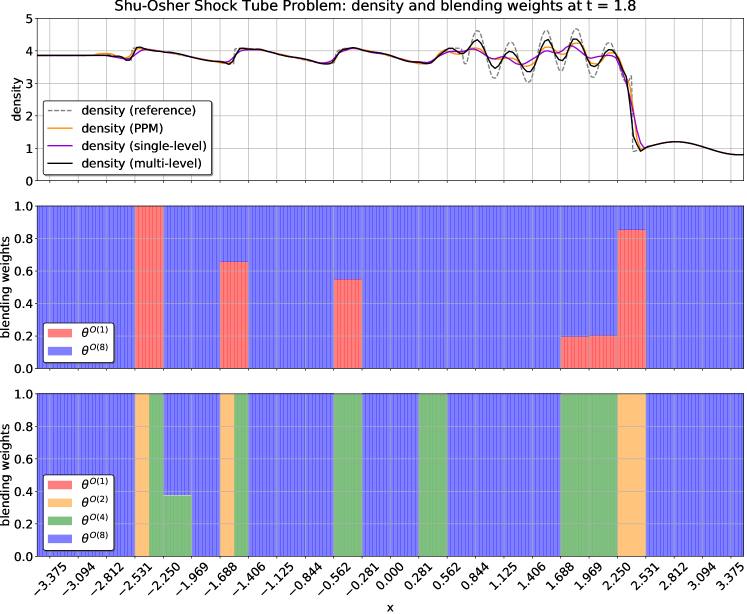
Figure 8: Shu-Osher Shock Tube Problem: Numerical solution of the density profile (top row) with the DGFV8 multi-level blending scheme together with the reference solution (PPM on 2048 DOF), PPM and single-level blending scheme all using 256 DOF. The center row shows the blending weights $\theta^{\mathcal{O}(n)}$ (eq. (3.4)) for the single-level blending while the bottom row shows the multi-level blending. The vertical grid lines depict the element boundaries.

3.5 2D Riemann Problems

In this section we present a selection of three 2D Riemann problems [43, 53, 40]. The domain for all simulations is set to $\Omega=[-0.5,0.5]^{2}$ with a uniform grid resolution of $64^{2}$ elements, respectively $512^{2}$ DOF. The setup consists of the four quadrants each initialized with their own constant states. The exact parameters of each Riemann problem are given in [43] where they are addressed with a fixed configuration number. For brevity we omit the setup parameters and refer to [43]. In this work we show configurations 3, 4 and 6. We are interested in the change of the numerical solution when we incrementally add one level of blending order from one run to the next. Hence, we present three solutions for each 2D Riemann problem denoted by their respective multi-level schemes: DGFV2, DGFV4 and DGFV8. Note that the schemes are implemented in such a way that they operate on the same element size of $N^{2}=8^{2}$ mean values. The results are shown in Fig 9 to 11. The left column shows the density contour and the right column the weighted blending factors as in (57). The general observation is that with increasing order there is more structure visible in the density plots and the blending patterns get more nuanced in tracing the flow structures.

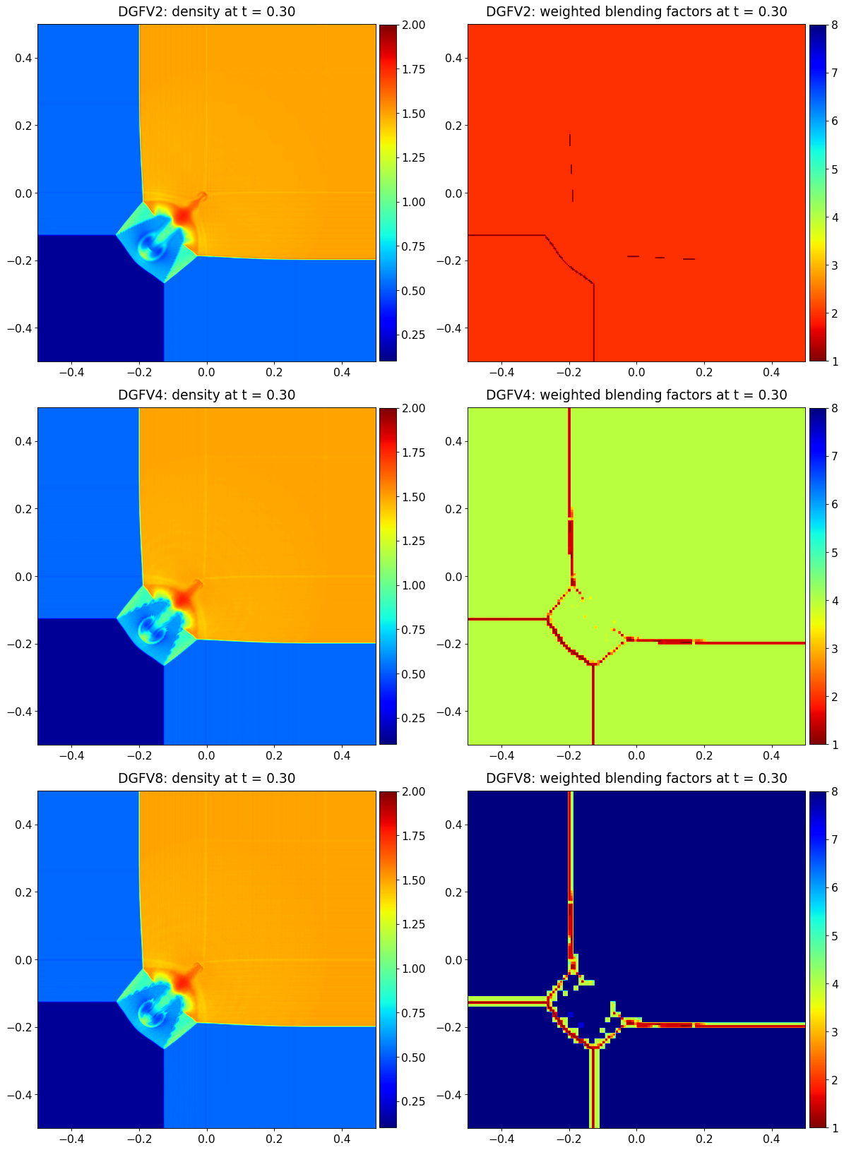
Figure 9: 2D Riemann problem (configuration 3, see [43]) computed with the (from top to bottom) DGFV2, DGFV4 and DGFV8 scheme. The resolution of $512^{2}$ DOF is the same for all runs. Left: density contours at final time $T=0.3$. Right: Weighted blending factors as defined in (57). Dark blue represents the full eighth order DG and dark red the full first order FV scheme.

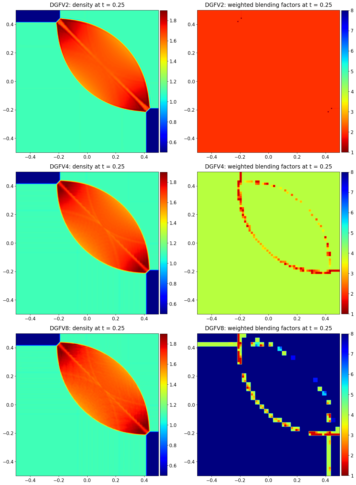
Figure 10: 2D Riemann problem (configuration 4, see [43]) computed with the (from top to bottom) DGFV2, DGFV4 and DGFV8 scheme. The resolution of $512^{2}$ DOF is the same for all runs. Left: density contours at final time $T=0.25$. Right: Weighted blending factors as defined in (57). Dark blue represents the full eighth order DG and dark red the full first order FV scheme.

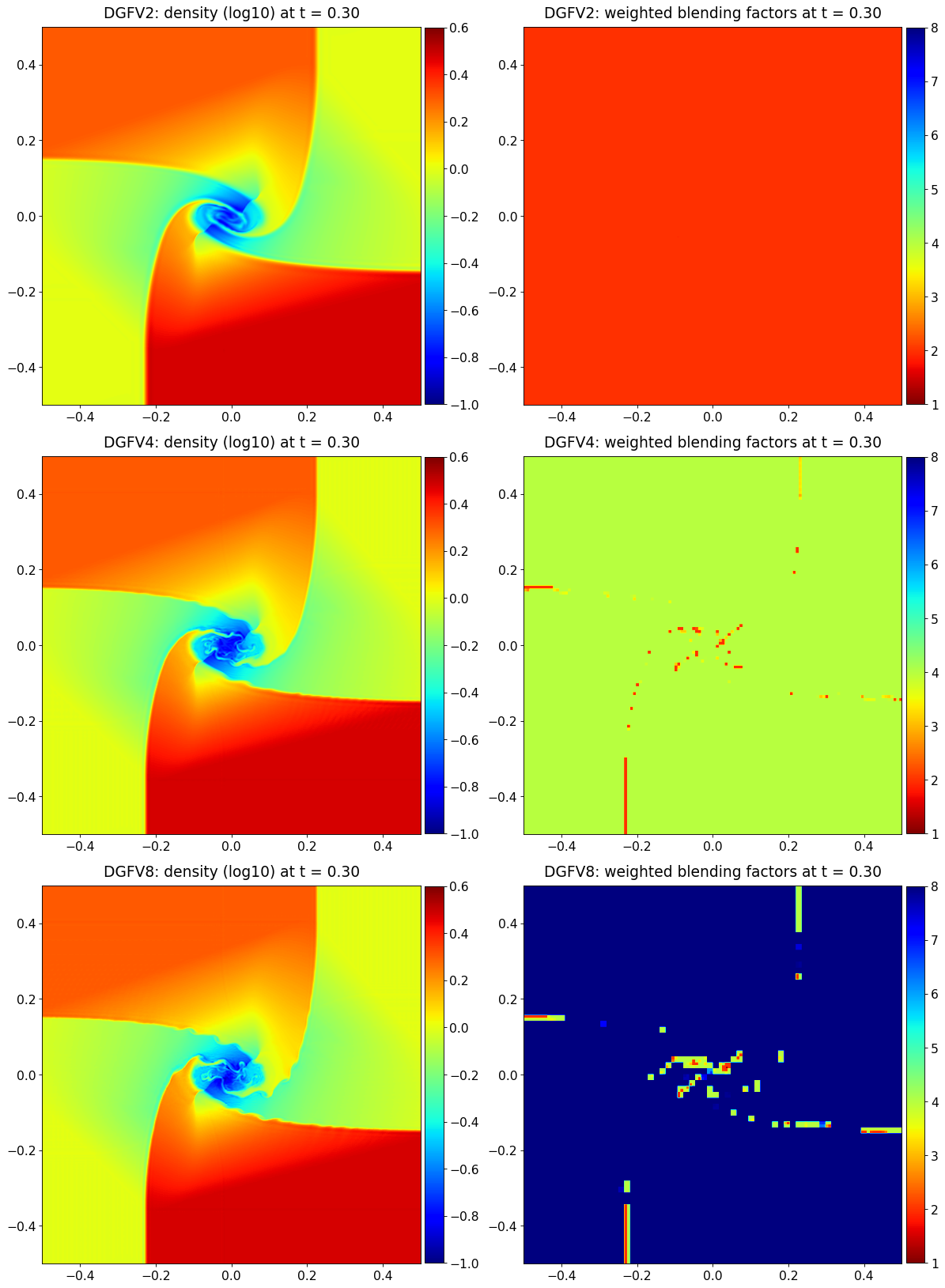
Figure 11: 2D Riemann problem (configuration 6, see [43]) computed with the (from top to bottom) DGFV2, DGFV4 and DGFV8 scheme. The resolution of $512^{2}$ DOF is the same for all runs. Left: density contours in log-scale at final time $T=0.3$. Right: Weighted blending factors as defined in (57). Dark blue represents the full eighth order DG and dark red the full first order FV scheme.

3.6 2D Sedov Blast

The Sedov blast problem [64, 65, 13] describes the self-similar evolution of a radially symmetrical blast wave from an initial pressure point (delta distribution) at the center into the surrounding, homogeneous medium. The analytical solution is given in [54, 39]. In our setup, we approximate the initial pressure point with a smooth Gaussian distribution

$$\mathcal{E}_{0}(\bm{x})=\frac{p_{0}}{\gamma-1}+\frac{E}{(2\,\pi\,\sigma^{2})^{d/2}}\,\exp{\Big{(}-\frac{1}{2}\,\frac{\bm{x}^{T}\bm{x}}{\sigma^{2}}\Big{)}},$$ (61)

with the spatial dimension $d=2$, the blast energy $E=1$ and the width $\sigma$ such that the initial Gaussian is reasonably resolved. The surrounding medium is initialized with $\rho_{0}=1$ and $p_{0}=10^{-14}$. Dimensional analysis [54] reveals that the analytical solution of the density right at the shock front is determined by

$$\rho_{\text{shock}}=\frac{\gamma+1}{\gamma-1}\,\rho_{0}.$$

With the adiabatic coefficient $\gamma=1.4$, we investigate how close the numerical results match $\rho_{\text{shock}}=6$. The Cartesian mesh has a FV equivalent uniform grid resolution of $512^{2}$ DOF, i.e. when computing with the full eighth order DG approximation space, the total number of DG elements is $64^{2}$. The spatial domain is $\Omega\in[-0.25,0.25]^{2}$ with the initial blast width $\sigma=5\times 10^{-3}$. We compare the accuracy of the results obtained with the single-level and the multi-level (DGFV8) blending discretizations as well as the PPM. Fig. 13 shows the shell-averaged density and pressure profiles at final time $T=0.05$. Fig. 12 presents the numerical solution over the whole domain as computed with the multi-level DGFV8. To further illustrate the behavior of the multi-level and single-level blending approach we also show in Fig. 14 the weighted blending factors along the x-axis. The shock front is much sharper for the multi-level blending compared to the single-level blending. It can be observed how the weighted blending factor is dominated by the first order FV scheme ($\bar{\alpha}\approx 1$) directly at the shock, but transitions quickly to a blended discretization ($1<\bar{\alpha}<8$) up to the full eighth order DG ($\bar{\alpha}\approx 8$) away from the shock, even within a single DG element. This behavior demonstrates the sub-element adaptivity of our novel approach. Again, similarly to the shock tube section 3.4 and the 2D Riemann problem section 3.5 the results for the 2D Sedov blast wave show the benefit of the multi-level approach, with the numerical profiles even slightly closer to $\rho_{\text{shock}}=6$ compared to the PPM with equal resolution of $512^{2}$ DOF.

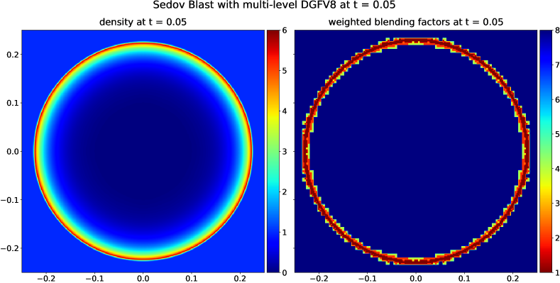
Figure 12: 2D Sedov Blast: Numerical solution computed with DGFV8 at final simulation time $T=0.05$. Left: density contours. Right: Weighted blending factors as defined in (57). Dark blue represents the full eighth order DG and dark red the full first order FV scheme.

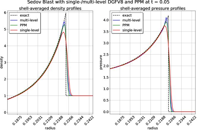
Figure 13: 2D Sedov Blast: shell-averaged density and pressure profiles at final simulation time $T=0.05$ computed with the single-/multi-level blending scheme (DGFV8) and PPM on a FV equivalent uniform grid resolution of $512^{2}$ DOF. The vertical grid lines depict the element boundaries.

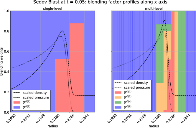
Figure 14: 2D Sedov Blast: We compare the blending factor profiles along the x-axis of the single- and multi-level blending schemes at final time $T=0.05$. The blending weights $\theta^{\mathcal{O}(n)}$ (eq. (3.4)) are encoded with stacked bars in their respective colors. The vertical grid lines highlight the eighth order DG element boundaries. For reference the scaled density ($\rho/6$) and scaled pressure ($p/5$) are included.

4 Simulation of a Young Supernova Remnant

Supernova models have been analyzed and discussed for many decades and since they unite a broad range of features such as strong shocks, instabilities and turbulence, they resemble a good test bed for our novel shock capturing approach in combination with AMR.

The general sequence of events of the presented supernova simulation is like this: We start with a constant distribution of very low density resembling interstellar media (ISM) that typically fills the space between stars. When a star explodes by turning into a supernova it ejects its own mass at very high speeds into the ISM preceded by a strong shock front heating up the ISM. The ejected mass is rapidly decelerated by the swept-up ISM giving rise to a so called reverse shock that travels backwards to the center. The interface, or more precisely the contact discontinuity, between shocked ejecta and shocked ISM is unstable and leads to a layer of slowly growing Rayleigh-Taylor instabilities. This gradually expanding layer, called supernova remnant, is of special interest since this is where astronomical observations reveal a lot of ongoing physics and chemistry, especially driven by mixing and turbulence.

We adapt the setup descriptions in [8, 19, 17] where we have the initial (internal) blast energy $E$ and the ejecta mass $M$ given in cgs (centimeter-gram-seconds) units. It is beneficial to convert the given units to convenient simulation units reflecting characteristic dimensions of the physical model at hand. Table 5 lists the conversion between cgs and simulation units and table 6 lists the initial parameters used in this simulation.

Table 5: Conversion from cgs units to simulation units.

quantity	cgs units	simulation units
mass	g	$\text{M}_{\odot}=1.989\times 10^{33}\,\text{g}$
time	s	$\text{yr}=3.154\times 10^{7}\,\text{s}$
length	cm	$\text{pc}=3.086\times 10^{18}\,\text{cm}$
temperature	K	K

Table 6: Hydrodynamical parameters in cgs units and simulation units.

description	cgs units	simulation units
domain size	$L=1.543\times 10^{19}\,\text{cm}$	$L=5\,\text{pc}$
blast energy	$E=10^{51}\text{erg}$	$E=5.2516\times 10^{-5}\,\text{M}_{\odot}\frac{\text{pc}^{2}}{\text{yr}^{2}}$
ejecta mass	$M=2.7846\times 10^{33}\,\text{g}$	$M=1.4\,\text{M}_{\odot}$
ambient density	$n_{H}=0.13\,\text{cm}^{-3}$	$\rho_{a}=2.4539\times 10^{-3}\,\frac{\text{M}_{\odot}}{\text{pc}^{3}}$
ambient temperature	$T=10^{4}\,\text{K}$	$p_{a}=2.1309\times 10^{-13}\,\frac{\text{M}_{\odot}}{\text{pc}\,\text{yr}^{2}}$

The ambient density $\rho_{a}$ is related to the mono-atomic particle (hydrogen) density $n_{H}$ via $\rho_{a}=m_{u}\,n_{H}$, where $m_{u}$ is $\frac{1}{12}$ of the mass of a carbon-12 atom. The ambient pressure $p_{a}$ is calculated from the ideal gas law, i.e. $p_{a}=n_{H}\,k_{B}\,T$ with the Boltzmann constant $k_{B}$. There is some ambiguity regarding the ambient gas temperature $T$. The literature mentions a warm and neutral interstellar medium which is attributed to temperatures between $6\times 10^{3}\,\text{K}$ and $10^{4}\,\text{K}$. The heat capacity ratio is fixed to $\gamma=5/3$. The simulation time spans a period from $t_{0}=10\,\text{yr}$ to $T=500\,\text{yr}$. The expansion of the forward shock (eq. (64)) is then expected to approximately reach $R_{\text{FS}}=5\,\text{pc}$, which determines the size of the computational domain $L:=5\,\text{pc}$. Fig. 15 depicts a schematic of the simulation setup. Due to the rotational symmetry of the setup it is sufficient to simulate just one octant of the supernova.

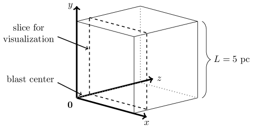
Figure 15: Computational domain (cubic box) covering one octant of the supernova model. The faces at the coordinate axes are set to reflecting walls while the opposite sides are set to outflow.

The following formulas have been derived in [8] and were adapted to the current setup, i.e. power-law indices of $(s,n)=(0,7)$. The self-similar solution at initial time $t_{0}=10\,\text{yr}$ within the power law region, respectively the blast center, is given by

$$r(t)=t\;\sqrt{\frac{5}{3}\,\frac{E}{M}}\quad\text{and}\quad\rho(t)=\frac{25}{21\,\pi}\;\frac{E^{2}}{M}\,t^{4}\,r(t)^{-7}.$$ (62)

We initialize the density as

$$\rho_{0}(\bm{x})=\rho_{a}+\rho(t_{0})\cdot\left\{\;\begin{aligned} &\quad\;\;\;1,&\quad|\bm{x}|\leq r(t_{0}),\\ &\left(\frac{|\bm{x}|}{r(t_{0})}\right)^{-7},&\quad|\bm{x}|>r(t_{0}),\end{aligned}\right.$$ (63)

and the total energy with (61) where $p_{0}=p_{a}$, $d=3$ and $\sigma=\frac{3}{4}\,r(t_{0})$. The initial momentum is $(\rho\,\bm{v})_{0}=\bm{0}$. Since we are only interested in the evolution of the instability layer of the supernova we apply the following rules for mesh refinement and coarsening. The expansion radius of the forward shock over time is given by

$$R_{\text{FS}}(t)=1.06\left(\frac{E^{2}}{M\,\rho_{a}}\right)^{1/7}\,t^{4/7}.$$ (64)

This allows us to assign an adaptive, high resolution shell of maximal refined elements following the remnant as it expands into the computational domain. The inner and outer radii of the shell are estimated as

$$R_{\text{inner}}(t)=0.7\,R_{\text{FS}}(t)\quad\text{and}\quad R_{\text{outer}}(t)=1.15\,R_{\text{FS}}(t),$$ (65)

which have been found adequate via numerical experimentation. Moreover, up to $t=200\,\text{yr}$ we enforce $R_{\text{inner}}=0$, which ensures that the first phase of the explosion is well resolved in any case. The refinement levels range from 2 to 6, which translates to a FV equivalent resolution from $2^{2}\cdot 8=16$ up to $2^{6}\cdot 8=512$ cells in each spatial direction.

We perform three simulations with the 3D multi-level blending schemes DGFV2, DGFV4 and DGFV8, analog to the 2D Riemann problems discussed in section 3.5. Fig. 16 shows the density slice (left column) sketched in Fig. 15 at the final simulation time of $T=500\,\text{yr}$, while Fig. 17 shows the corresponding 3D density contour rendering of the DGFV8 solution. The shock front partially left the domain, which is not considered a problem since the region of interest, namely the instability layer, is still completely covered. The areas of no interest, i.e. the outer region as well as the center, are only coarsely resolved by the AMR scheme. Clearly, an increase in order leads to a much more detailed remnant structure emphasizing the advantage of higher order schemes in resolving small scale turbulence driven by Rayleigh-Taylor instability, see [8]. The weighted blending factor is shown in the right column of Fig. 16. The band of highly refined elements is clearly visible following the remnant as intended. Two distinctive lines of blending activity trace the front and reverse shocks. The plots also show a strong qualitative difference of the amount of scales in the instability layer for DGFV2 and DGFV4. Clearly, the DGFV4 result features more scales and finer structures as the DGFV2 simulation with the same FV equivalent grid resolution. The difference in scales between DGFV4 and DGFV8 is less pronounced which is probably related to the extensive blending activity with O4 inside the instability layer of the DGFV8 simulation. In this turbulent part we suspect that the standard collocation eighth order DG scheme might face aliasing instability issues as described in the introduction. There are techniques to reduce aliasing issues available, such as filtering, consistent integration and split-forms. However, this aspect is not the main topic of the paper and it is interesting to see, that the multi-level blending automatically adjusts to cope with these issues as well.

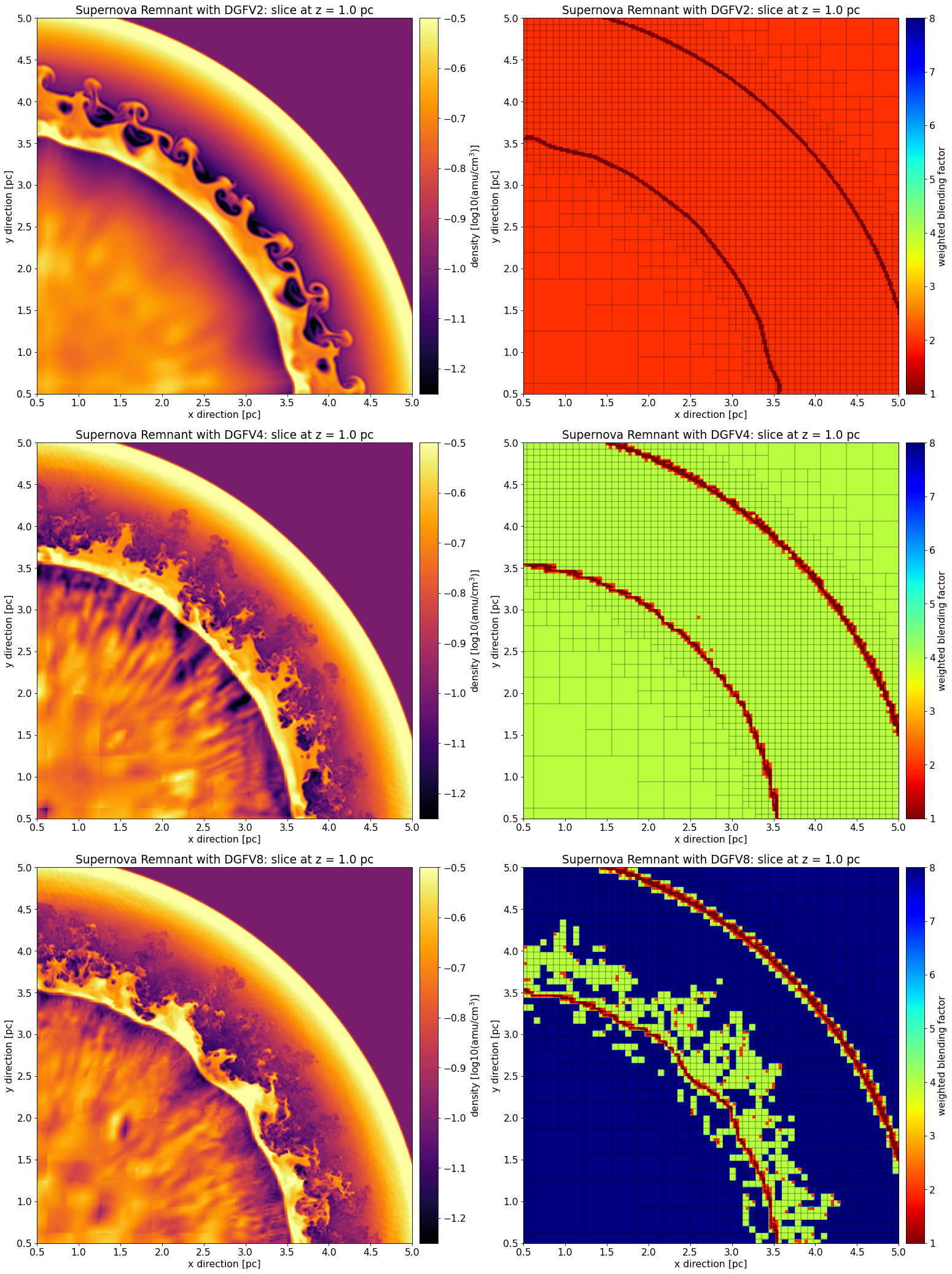
Figure 16: left column: 2D density slice (see figure 15) showing the instability region respectively remnant of the supernova at $T=500\,\text{yr}$ simulated with the (from top to bottom) DGFV2, DGFV4 and DGFV8 scheme. right column: 2D slice of the weighted blending factors of the respective blending schemes at $T=500\,\text{yr}$. The black lines correspond to the element boundaries of the Cartesian non-conforming mesh.

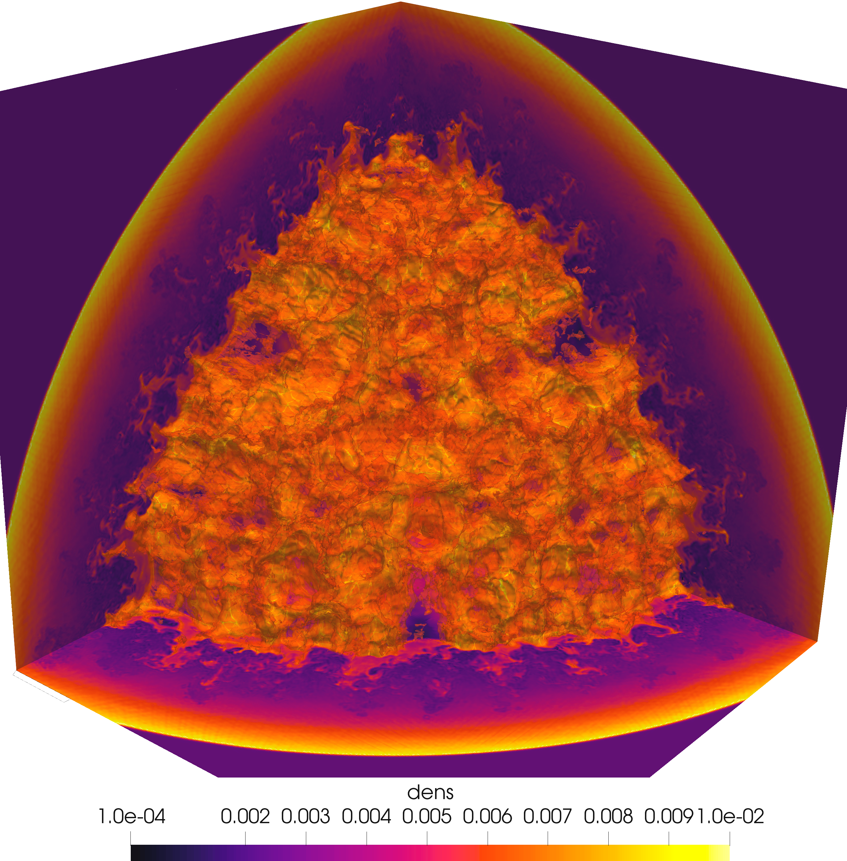
Figure 17: 3D density contour rendering showing the instability region respectively remnant of the supernova at final simulation time $T=500\,\text{yr}$ simulated with the DGFV8 scheme.

5 Conclusion

In this work, we introduce an adaptive sub-element based shock capturing approach for DG methods. We interpret an element first as a collection of piecewise constant data. This set of piecewise constant data can be interpreted and reconstructed in a variety of ways. We focus on piecewise polynomial approximation spaces, starting from a pure piecewise constant FV type interpretation (no reconstruction) up to the fully maximum order polynomial reconstruction and every combination in-between, e.g. piecewise linear and piecewise cubic reconstructions. In a second step, we link the data interpretation to a corresponding (high order) DG discretization. Thus, we get a hierarchy of discretizations acting on the same set of data.

The idea is then to adaptively blend this hierarchy of different discretization, where the low order variants are chosen close to discontinuities and the high order variants in smooth or turbulent parts of the simulation. Instead of having an element based troubled cell indicator approach, we use the different data interpretations again to compute sub-element localized indicators, which allows for a sub-element adaptive blending of the discretizations. When the blending can change throughout the element, special care is necessary to preserve exact conservation of the resulting multi-level blended discretization. We achieve exact conservation, by introducing unique, blended reconstruction states at subcell and sub-element interfaces.

In our prototype implementation, we further demonstrate that a natural combination of this sub-element adaptive approach is with adaptive mesh refinement. We base the AMR implementation on the p4est Octree library, which allows for a straight forward parallelization of the whole computational framework.

We show standard numerical test cases to validate the new approach and a simplified model of a supernova remnant to highlight its high accuracy for challenging test cases with strong shocks and turbulence like structures.

6 APPENDIX

6.1 Four levels of data interpretation of $8$ mean values

6.2 Boundary Evaluation Operators for the Multi-level Blending Scheme (2.6).

$$\left[\bm{\mathds{1}}_{4}\otimes\hat{\bm{B}}^{\mathcal{O}(2)}\right]^{(0)}=\left(\begin{array}[]{*{9}{@{}C{\mycolwd}@{}}}\hat{B}^{\mathcal{O}(2)}_{1\,1}$\@add@centering&0$\@add@centering&\hat{B}^{\mathcal{O}(2)}_{1\,3}$\@add@centering&0$\@add@centering&0$\@add@centering&0$\@add@centering&0$\@add@centering&0$\@add@centering&0$\@add@centering\cr[2mm]\hat{B}^{\mathcal{O}(2)}_{2\,1}$\@add@centering&0$\@add@centering&\hat{B}^{\mathcal{O}(2)}_{2\,3}$\@add@centering&0$\@add@centering&0$\@add@centering&0$\@add@centering&0$\@add@centering&0$\@add@centering&0$\@add@centering\cr[2mm]0$\@add@centering&0$\@add@centering&\hat{B}^{\mathcal{O}(2)}_{1\,1}$\@add@centering&0$\@add@centering&\hat{B}^{\mathcal{O}(2)}_{1\,3}$\@add@centering&0$\@add@centering&0$\@add@centering&0$\@add@centering&0$\@add@centering\cr[2mm]0$\@add@centering&0$\@add@centering&\hat{B}^{\mathcal{O}(2)}_{2\,1}$\@add@centering&0$\@add@centering&\hat{B}^{\mathcal{O}(2)}_{2\,3}$\@add@centering&0$\@add@centering&0$\@add@centering&0$\@add@centering&0$\@add@centering\cr[2mm]0$\@add@centering&0$\@add@centering&0$\@add@centering&0$\@add@centering&\hat{B}^{\mathcal{O}(2)}_{1\,1}$\@add@centering&0$\@add@centering&\hat{B}^{\mathcal{O}(2)}_{1\,3}$\@add@centering&0$\@add@centering&0$\@add@centering\cr[2mm]0$\@add@centering&0$\@add@centering&0$\@add@centering&0$\@add@centering&\hat{B}^{\mathcal{O}(2)}_{2\,1}$\@add@centering&0$\@add@centering&\hat{B}^{\mathcal{O}(2)}_{2\,3}$\@add@centering&0$\@add@centering&0$\@add@centering\cr[2mm]0$\@add@centering&0$\@add@centering&0$\@add@centering&0$\@add@centering&0$\@add@centering&0$\@add@centering&\hat{B}^{\mathcal{O}(2)}_{1\,1}$\@add@centering&0$\@add@centering&\hat{B}^{\mathcal{O}(2)}_{1\,3}$\@add@centering\cr[2mm]0$\@add@centering&0$\@add@centering&0$\@add@centering&0$\@add@centering&0$\@add@centering&0$\@add@centering&\hat{B}^{\mathcal{O}(2)}_{2\,1}$\@add@centering&0$\@add@centering&\hat{B}^{\mathcal{O}(2)}_{2\,3}$\@add@centering\end{array}\right)\;\in\mathbb{R}^{8\times 9}$$

$$\left[\bm{\mathds{1}}_{2}\otimes\hat{\bm{B}}^{\mathcal{O}(4)}\right]^{(0)}=\left(\begin{array}[]{*{9}{@{}C{\mycolwd}@{}}}\hat{B}^{\mathcal{O}(4)}_{1\,1}$\@add@centering&0$\@add@centering&0$\@add@centering&0$\@add@centering&\hat{B}^{\mathcal{O}(4)}_{1\,5}$\@add@centering&0$\@add@centering&0$\@add@centering&0$\@add@centering&0$\@add@centering\cr[2mm]\hat{B}^{\mathcal{O}(4)}_{2\,1}$\@add@centering&0$\@add@centering&0$\@add@centering&0$\@add@centering&\hat{B}^{\mathcal{O}(4)}_{2\,5}$\@add@centering&0$\@add@centering&0$\@add@centering&0$\@add@centering&0$\@add@centering\cr[2mm]\hat{B}^{\mathcal{O}(4)}_{3\,1}$\@add@centering&0$\@add@centering&0$\@add@centering&0$\@add@centering&\hat{B}^{\mathcal{O}(4)}_{3\,5}$\@add@centering&0$\@add@centering&0$\@add@centering&0$\@add@centering&0$\@add@centering\cr[2mm]\hat{B}^{\mathcal{O}(4)}_{4\,1}$\@add@centering&0$\@add@centering&0$\@add@centering&0$\@add@centering&\hat{B}^{\mathcal{O}(4)}_{4\,5}$\@add@centering&0$\@add@centering&0$\@add@centering&0$\@add@centering&0$\@add@centering\cr[2mm]0$\@add@centering&0$\@add@centering&0$\@add@centering&0$\@add@centering&\hat{B}^{\mathcal{O}(4)}_{1\,1}$\@add@centering&0$\@add@centering&0$\@add@centering&0$\@add@centering&\hat{B}^{\mathcal{O}(4)}_{1\,5}$\@add@centering\cr[2mm]0$\@add@centering&0$\@add@centering&0$\@add@centering&0$\@add@centering&\hat{B}^{\mathcal{O}(4)}_{2\,1}$\@add@centering&0$\@add@centering&0$\@add@centering&0$\@add@centering&\hat{B}^{\mathcal{O}(4)}_{2\,5}$\@add@centering\cr[2mm]0$\@add@centering&0$\@add@centering&0$\@add@centering&0$\@add@centering&\hat{B}^{\mathcal{O}(4)}_{3\,1}$\@add@centering&0$\@add@centering&0$\@add@centering&0$\@add@centering&\hat{B}^{\mathcal{O}(4)}_{3\,5}$\@add@centering\cr[2mm]0$\@add@centering&0$\@add@centering&0$\@add@centering&0$\@add@centering&\hat{B}^{\mathcal{O}(4)}_{4\,1}$\@add@centering&0$\@add@centering&0$\@add@centering&0$\@add@centering&\hat{B}^{\mathcal{O}(4)}_{4\,5}$\@add@centering\end{array}\right)\;\in\mathbb{R}^{8\times 9}$$

$$\left[\bm{\mathds{1}}_{1}\otimes\hat{\bm{B}}^{\mathcal{O}(8)}\right]^{(0)}=\left(\begin{array}[]{*{9}{@{}C{\mycolwd}@{}}}\hat{B}^{\mathcal{O}(8)}_{1\,1}$\@add@centering&0$\@add@centering&0$\@add@centering&0$\@add@centering&0$\@add@centering&0$\@add@centering&0$\@add@centering&0$\@add@centering&\hat{B}^{\mathcal{O}(8)}_{1\,9}$\@add@centering\cr[2mm]\hat{B}^{\mathcal{O}(8)}_{2\,1}$\@add@centering&0$\@add@centering&0$\@add@centering&0$\@add@centering&0$\@add@centering&0$\@add@centering&0$\@add@centering&0$\@add@centering&\hat{B}^{\mathcal{O}(8)}_{2\,9}$\@add@centering\cr[2mm]\hat{B}^{\mathcal{O}(8)}_{3\,1}$\@add@centering&0$\@add@centering&0$\@add@centering&0$\@add@centering&0$\@add@centering&0$\@add@centering&0$\@add@centering&0$\@add@centering&\hat{B}^{\mathcal{O}(8)}_{3\,9}$\@add@centering\cr[2mm]\hat{B}^{\mathcal{O}(8)}_{4\,1}$\@add@centering&0$\@add@centering&0$\@add@centering&0$\@add@centering&0$\@add@centering&0$\@add@centering&0$\@add@centering&0$\@add@centering&\hat{B}^{\mathcal{O}(8)}_{4\,9}$\@add@centering\cr[2mm]\hat{B}^{\mathcal{O}(8)}_{5\,1}$\@add@centering&0$\@add@centering&0$\@add@centering&0$\@add@centering&0$\@add@centering&0$\@add@centering&0$\@add@centering&0$\@add@centering&\hat{B}^{\mathcal{O}(8)}_{5\,9}$\@add@centering\cr[2mm]\hat{B}^{\mathcal{O}(8)}_{6\,1}$\@add@centering&0$\@add@centering&0$\@add@centering&0$\@add@centering&0$\@add@centering&0$\@add@centering&0$\@add@centering&0$\@add@centering&\hat{B}^{\mathcal{O}(8)}_{6\,9}$\@add@centering\cr[2mm]\hat{B}^{\mathcal{O}(8)}_{7\,1}$\@add@centering&0$\@add@centering&0$\@add@centering&0$\@add@centering&0$\@add@centering&0$\@add@centering&0$\@add@centering&0$\@add@centering&\hat{B}^{\mathcal{O}(8)}_{7\,9}$\@add@centering\cr[2mm]\hat{B}^{\mathcal{O}(8)}_{8\,1}$\@add@centering&0$\@add@centering&0$\@add@centering&0$\@add@centering&0$\@add@centering&0$\@add@centering&0$\@add@centering&0$\@add@centering&\hat{B}^{\mathcal{O}(8)}_{8\,9}$\@add@centering\end{array}\right)\;\in\mathbb{R}^{8\times 9}$$

6.3 Extension to 3D Cartesian Grids

The extension to higher spatial dimensions with Cartesian conforming grids is relatively straight forward via a tensor-product strategy. In this section we want to present the most important building blocks for the 3D single-level blending scheme. The steps of the 3D multi-level blending are analogous as in section 2.6 and not detailed any further. Consider the general 3D conservation law

$$\partial_{t}u+\partial_{x}f(u)+\partial_{y}g(u)+\partial_{z}h(u)=0.$$ (66)

We now have an element $q$ with $N^{3}$ mean values as available data

$$\mathbf{\bar{u}}_{q}\in\mathbb{R}^{N\times N\times N},$$

and the element sizes $\Delta x_{q}$, $\Delta y_{q}$ and $\Delta z_{q}$. With the tensor-product of Lagrange polynomials $\ell$ on Legendre-Gauss nodes $\xi_{i}$, $i=1,\ldots,N$,

$$u(t;\xi,\eta,\zeta)\approx\sum_{i,j,k=1}^{N}\tilde{u}_{ijk}(t)\,\ell_{i}(\xi)\,\ell_{j}(\eta)\,\ell_{k}(\zeta),$$ (67)

and the reconstruction operator $\bm{R}$, which we introduced in section 2.4, we get the nodal coefficients as

$$\mathbf{\tilde{u}}_{q}=\mathbf{\bar{u}}_{q}\bigtimes_{d=x}^{z}\bm{R}=\mathbf{\bar{u}}_{q}\times_{x}\bm{R}\times_{y}\bm{R}\times_{z}\bm{R}\quad\in\mathbb{R}^{N\times N\times N}.$$ (68)

Here we make use of the n-mode product notation [34]. A definition is given in appendix 6.5. In general all vector and matrix operations presented so far can be directly expanded to 3D via the n-mode product. The blending scheme (42) in 3D reads as

$$\mathbf{\partial_{t}\bar{u}}_{q}=- \,(1-\alpha_{q})\,\frac{N}{\Delta x_{q}}\,\mathbf{\bar{f}}_{q}^{*}\times_{x}\bm{\Delta}+\,\alpha_{q}\,\frac{1}{\Delta x_{q}}\,\Big{\{}\mathbf{\tilde{f}}_{q}\times_{x}\hat{\bm{D}}\times_{y}\bm{P}\times_{z}\bm{P}-\mathbf{\bar{f}}_{q}^{*}\times_{x}\hat{\bm{B}}\Big{\}}$$

$$- \,(1-\alpha_{q})\,\frac{N}{\Delta y_{q}}\,\mathbf{\bar{g}}_{q}^{*}\times_{y}\bm{\Delta}+\,\alpha_{q}\,\frac{1}{\Delta y_{q}}\,\Big{\{}\mathbf{\tilde{g}}_{q}\times_{y}\hat{\bm{D}}\times_{z}\bm{P}\times_{x}\bm{P}-\mathbf{\bar{g}}_{q}^{*}\times_{y}\hat{\bm{B}}\Big{\}}$$ (69)

$$- \,(1-\alpha_{q})\,\frac{N}{\Delta z_{q}}\,\mathbf{\bar{h}}_{q}^{*}\times_{z}\bm{\Delta}+\,\alpha_{q}\,\frac{1}{\Delta z_{q}}\,\Big{\{}\mathbf{\tilde{h}}_{q}\times_{z}\hat{\bm{D}}\times_{x}\bm{P}\times_{y}\bm{P}-\mathbf{\bar{h}}_{q}^{*}\times_{z}\hat{\bm{B}}\Big{\}}.$$

The DG volume fluxes are calculated from the node values as

$$\left(\mathbf{\tilde{f}}_{q}\right)_{ijk}=f\left(\left(\mathbf{\tilde{u}}_{q}\right)_{ijk}\right),\;\left(\mathbf{\tilde{g}}_{q}\right)_{ijk}=g\left(\left(\mathbf{\tilde{u}}_{q}\right)_{ijk}\right)\;\text{and}\;\left(\mathbf{\tilde{h}}_{q}\right)_{ijk}=h\left(\left(\mathbf{\tilde{u}}_{q}\right)_{ijk}\right),\;i,j,k=1,\ldots,N.$$

Remark: If necessary, the $\beta$-reconstruction (30) ensures permissible states for the reconstructed polynomial, i.e.

$$\mathbf{\tilde{u}}_{q}^{(\beta)}=\mathbf{\bar{u}}_{q}\bigtimes_{d=x}^{z}\bm{R}^{(\beta)}.$$ (70)

Again, for $\mathbf{\bar{f}}_{q}^{*}\in\mathbb{R}^{(N+1)\times N\times N}$, $\mathbf{\bar{g}}_{q}^{*}\in\mathbb{R}^{N\times(N+1)\times N}$ and $\mathbf{\bar{h}}_{q}^{*}\in\mathbb{R}^{N\times N\times(N+1)}$, we need to compute common surface fluxes in order to preserve conservation. Therefore, we define two selection operators,

$$\bm{s}^{-}=(1,0,\ldots,0,0)^{T}\in\mathbb{R}^{N}\quad\text{and}\quad\bm{s}^{+}=(0,0,\ldots,0,1)^{T}\in\mathbb{R}^{N},$$

mapping the outermost mean values of $\mathbf{\bar{u}}_{q}$ to the respective interface. Then the 3D analogue of the prolongation procedure (37) along direction $d$ reads as

$$\bar{\mathfrak{u}}_{q\pm\frac{1}{2}}^{\pm d}=(1-\alpha_{q})\;\;\underbrace{\mathbf{\bar{u}}_{q}\times_{d}\bm{s}^{\pm}}_{\mathclap{\begin{subarray}{c}\text{face centered}\\ \text{mean values}\end{subarray}}}\quad+\quad\alpha_{q}\;\;\underbrace{\bm{P}\overbrace{\left(\mathbf{\tilde{u}}_{q}\times_{d}\bm{b}^{\pm}\right)}^{\begin{subarray}{c}\text{nodal boundary}\\ \text{values}\end{subarray}}\bm{P}^{T}}_{\mathclap{\begin{subarray}{c}\text{face centered}\\ \text{mean values}\end{subarray}}}\;\>\;\;\in\mathbb{R}^{N\times N}.$$ (71)

In Fig. 19 the two kinds of boundary values are illustrated.

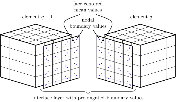
Figure 19: Schematic of conforming interface $q-\frac{1}{2}$ with 1:1 adjacent elements $q-1$ and $q$ for $N=4$. The two kinds of boundary values occurring in (71) are illustrated.

Note that only the face centered mean values $\bar{\mathfrak{u}}_{q\pm\frac{1}{2}}^{\pm d}$ together with the blending factor $\alpha_{q}$ are supposed to be exchanged between processes in case of distributed computing.

Next, we reconstruct again a nodal representation from $\bar{\mathfrak{u}}_{q\pm\frac{1}{2}}^{\pm d}$

$$\tilde{\mathfrak{u}}_{q\pm\frac{1}{2}}^{\pm d}=\underbrace{\bm{R}\;\bar{\mathfrak{u}}_{q\pm\frac{1}{2}}^{\pm d}\;\bm{R}^{T}}_{\mathclap{\begin{subarray}{c}\text{nodal boundary}\\ \text{values}\end{subarray}}}\;\>\;\;\in\mathbb{R}^{N\times N}.$$ (72)

From the two representations of boundary values $\bar{\mathfrak{u}}_{q\pm\frac{1}{2}}^{\pm x}$ and $\tilde{\mathfrak{u}}_{q\pm\frac{1}{2}}^{\pm x}$ we calculate two candidate fluxes at the interface $q-\frac{1}{2}$. In x-direction it reads as

$$\bar{\mathfrak{f}}_{q-\frac{1}{2}}^{*^{\prime}}=f^{*}\left(\bar{\mathfrak{u}}_{q-\frac{1}{2}}^{+x},\bar{\mathfrak{u}}_{q-\frac{1}{2}}^{-x}\right)\;\>\;\;\in\mathbb{R}^{N\times N},$$ (73)

$$\tilde{\mathfrak{f}}_{q-\frac{1}{2}}^{*}=f^{*}\left(\tilde{\mathfrak{u}}_{q-\frac{1}{2}}^{+x},\tilde{\mathfrak{u}}_{q-\frac{1}{2}}^{-x}\right)\;\>\;\;\in\mathbb{R}^{N\times N}.$$ (74)

Next, we determine a common surface flux $\bar{\mathfrak{f}}_{q-\frac{1}{2}}^{*}$ by blending the two candidate interface fluxes

$$\bar{\mathfrak{f}}_{q-\frac{1}{2}}^{*}=(1-\alpha_{q-\frac{1}{2}})\;\;\bar{\mathfrak{f}}_{q-\frac{1}{2}}^{*^{\prime}}\;\;+\;\;\alpha_{q-\frac{1}{2}}\;\;\bm{P}\;\tilde{\mathfrak{f}}_{q-\frac{1}{2}}^{*}\;\bm{P}^{T}\;\>\;\;\in\mathbb{R}^{N\times N},$$ (75)

where $\alpha_{q-\frac{1}{2}}=\frac{\alpha_{q-1}+\alpha_{q}}{2}$. The final step is to calculate the inner interface fluxes analogous to (38)

$$\left(\mathbf{\bar{f}}_{q}^{*}\right)_{ijk}=f^{*}(\bar{u}_{i-1jk},\bar{u}_{ijk}),\quad i=2,\ldots,N,\;j,k=1,\ldots,N$$

and insert the common surface fluxes $\bar{\mathfrak{f}}_{q\pm\frac{1}{2}}^{*}$

$$\left(\mathbf{\bar{f}}_{q}^{*}\right)_{ijk} =\left(\bar{\mathfrak{f}}_{q-\frac{1}{2}}^{*}\right)_{jk},\quad i=1,\;j,k=1,\ldots,N$$

$$\left(\mathbf{\bar{f}}_{q}^{*}\right)_{ijk} =\left(\bar{\mathfrak{f}}_{q+\frac{1}{2}}^{*}\right)_{jk},\quad i=N+1,\;j,k=1,\ldots,N.$$

The y- and z-direction are treated analogously. The computation of the blending parameter $\alpha$ for 3D follows the same steps as in section 2.7 where the integrals (49) are rewritten in 3D form. The presented parameters $\tau_{a}$ and $\tau_{s}$ stay the same. This concludes the 3D blending scheme with conforming interfaces.

We extend the 3D single-blending scheme to non-conforming grids where we assume 4:1 transitions only. See Fig. 20. The steps for the 3D multi-level blending scheme are analogous and not detailed any further. First, we define four matrix operators which allow us to construct refinement and coarsening procedures within the blending framework. We require that $N=2^{l},\,l\in\mathbb{N}$, and define the following expansion and compression operators

$$\bm{E}^{(N\rightarrow 2N)}:=\bm{\mathds{1}}_{N}\otimes\bm{1}_{2}\;\;\in\mathbb{R}^{2N\times N}$$ (76)

and

$$\bm{C}^{(N\rightarrow\tfrac{N}{2})}:=\frac{1}{2}\,\bm{\mathds{1}}_{N}\otimes\bm{1}_{2}^{T}\;\;\in\mathbb{R}^{\tfrac{N}{2}\times N}.$$ (77)

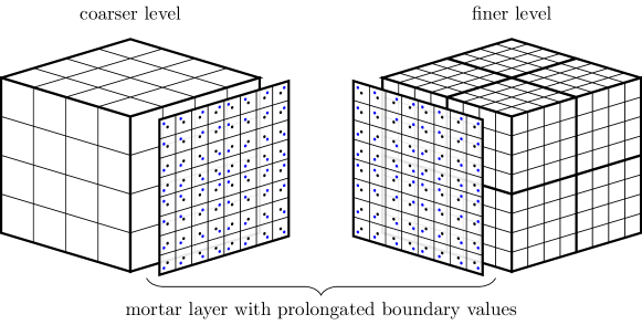
Figure 20: Schematic of a non-conforming interface with 4:1 adjacent cells for $N=4$. The two kinds of boundary values occurring in (80) are illustrated. Compare with Fig. 19.

Moreover, we need the projection operator $\bm{P}^{(N\rightarrow M)}$ introduced in section 2.3 for mapping $N$ node values to $M$ mean values. We define:

$$\underbrace{\bm{E}:=\bm{E}^{(N\rightarrow 2N)},\quad\bm{C}:=\bm{C}^{(N\rightarrow\tfrac{N}{2})}}_{\text{mean values to mean values}}\quad\text{and}\quad\underbrace{\bm{Z}:=\bm{P}^{(N\rightarrow 2N)},\quad\bm{Q}:=\bm{P}^{(N\rightarrow\tfrac{N}{2})}}_{\text{node values to mean values}}.$$

We refine the parent element $q$ as

$$\mathbf{\bar{r}}_{q}=(1-\alpha_{q})\,\mathbf{\bar{u}}_{q}\,\bigtimes_{d=x}^{z}\,\bm{E}+\alpha_{q}\,\mathbf{\tilde{u}}_{q}\,\bigtimes_{d=x}^{z}\,\bm{Z}\;\;\in\mathbb{R}^{2N\times 2N\times 2N}.$$ (78)

The refined block $\mathbf{\bar{r}}_{q}$ is then split into $8$ child elements. The reverse operation, namely coarsening, is done by compressing each child element $\mathbf{\bar{u}}_{r},\;r=1,\ldots,8$, separately:

$$\mathbf{\bar{c}}_{q}=(1-\alpha_{q})\,\mathbf{\bar{u}}_{q}\,\bigtimes_{d=x}^{z}\,\bm{C}+\alpha_{q}\,\mathbf{\tilde{u}}_{q}\,\bigtimes_{d=x}^{z}\,\bm{Q}\;\;\in\mathbb{R}^{\tfrac{N}{2}\times\tfrac{N}{2}\times\tfrac{N}{2}}.$$ (79)

Afterwards the family of $8$ blocks $\mathbf{\bar{c}}_{q}$ is glued together. These blending operations are especially useful for refining or coarsening of highly oscillatory data or at pronounced discontinuities.

For the treatment of non-conforming 4:1 interfaces we need a procedure which maps the boundary values from the coarser element to a so-called mortar layer [35] that has the same resolution as the adjacent four smaller elements. See Fig. 20. To compute the mortar layer of the coarser element $q$, we formulate

$$\left(\mathfrak{\bar{u}}_{q\pm\frac{1}{2}}^{\pm d}\right)_{\text{coarse}}=(1-\alpha_{q})\,\underbrace{\bm{E}\,\big{(}\mathbf{\bar{u}}_{q}\times_{d}\bm{s}^{\pm}\big{)}\,\bm{E}^{T}}_{\mathclap{\begin{subarray}{c}\text{face centered}\\ \text{mean values}\end{subarray}}}+\;\alpha_{q}\,\underbrace{\bm{\tilde{Z}}\overbrace{\big{(}\mathbf{\tilde{u}}_{q}\times_{d}\bm{b}^{\pm}\big{)}}^{\begin{subarray}{c}\text{nodal boundary}\\ \text{values}\end{subarray}}\bm{\tilde{Z}}^{T}}_{\mathclap{\begin{subarray}{c}\text{face centered}\\ \text{mean values}\end{subarray}}}\;\>\in\mathbb{R}^{2N\times 2N}.$$ (80)

Note the similarity to the prolongation procedure for conforming interfaces (71). The coarse side of the mortar layer $\left(\mathfrak{\bar{u}}_{q\pm\frac{1}{2}}^{\pm d}\right)_{\text{coarse}}$ is split up to match the faces of the four finer elements $r=1,\ldots,4$. The boundary values of the smaller elements are constructed by applying (71) individually. Only the mortar layers together with the associated blending factors $\alpha_{r}$, $r=1,\ldots,4$, are supposed to be exchanged between processes in case of distributed computing. The separate computation of the interface fluxes $\mathfrak{\bar{f}}^{*}_{\text{fine},r}\in\mathbb{R}^{N\times N}$, $r=1,\ldots,4$, follows the formulas (72)-(75). While the resulting four fluxes can be directly copied back to the smaller faces without further treatment, they have to be mapped to the coarser side via $L^{2}$-projection [35]

$$\int_{-\frac{1}{2}}^{0}\int_{-\frac{1}{2}}^{0}\left(f^{*}_{\text{coarse}}-f^{*}_{\text{fine},1}\right)\phi\,d\xi\,d\eta+\int_{0}^{\frac{1}{2}}\int_{-\frac{1}{2}}^{0}\left(f^{*}_{\text{coarse}}-f^{*}_{\text{fine},2}\right)\phi\,d\xi\,d\eta$$

$$+ \int_{-\frac{1}{2}}^{0}\int_{0}^{\frac{1}{2}}\left(f^{*}_{\text{coarse}}-f^{*}_{\text{fine},3}\right)\phi\,d\xi\,d\eta+\int_{0}^{\frac{1}{2}}\int_{0}^{\frac{1}{2}}\left(f^{*}_{\text{coarse}}-f^{*}_{\text{fine},4}\right)\phi\,d\xi\,d\eta=0.$$

The integrals are evaluated in the reference space of the coarse face. Applying exact quadrature rules gives

$$\left(\mathfrak{\tilde{f}}^{*}_{\text{coarse}}\right)_{ij}= \sum_{kl}^{N}\left(\mathfrak{\tilde{f}}^{*}_{\text{fine},1}\right)_{kl}\ell_{i}\left(\frac{1}{2}\,\xi_{k}-\frac{1}{4}\right)\frac{\omega_{k}}{2\,\omega_{i}}\ell_{j}\left(\frac{1}{2}\,\eta_{l}-\frac{1}{4}\right)\frac{\omega_{l}}{2\,\omega_{j}}+$$

$$\sum_{kl}^{N}\left(\mathfrak{\tilde{f}}^{*}_{\text{fine},2}\right)_{kl}\ell_{i}\left(\frac{1}{2}\,\xi_{k}+\frac{1}{4}\right)\frac{\omega_{k}}{2\,\omega_{i}}\ell_{j}\left(\frac{1}{2}\,\eta_{l}-\frac{1}{4}\right)\frac{\omega_{l}}{2\,\omega_{j}}+$$

$$\sum_{kl}^{N}\left(\mathfrak{\tilde{f}}^{*}_{\text{fine},3}\right)_{kl}\ell_{i}\left(\frac{1}{2}\,\xi_{k}-\frac{1}{4}\right)\frac{\omega_{k}}{2\,\omega_{i}}\ell_{j}\left(\frac{1}{2}\,\eta_{l}+\frac{1}{4}\right)\frac{\omega_{l}}{2\,\omega_{j}}+$$

$$\sum_{kl}^{N}\left(\mathfrak{\tilde{f}}^{*}_{\text{fine},4}\right)_{kl}\ell_{i}\left(\frac{1}{2}\,\xi_{k}+\frac{1}{4}\right)\frac{\omega_{k}}{2\,\omega_{i}}\ell_{j}\left(\frac{1}{2}\,\eta_{l}+\frac{1}{4}\right)\frac{\omega_{l}}{2\,\omega_{j}},$$

where $i,j=1,\ldots,N$ and $\xi_{k}$, $\eta_{l}$ are the collocation nodes of the tensor-product (67). We translate above equation into matrix notation and get

$$\mathfrak{\tilde{f}}^{*}_{\text{coarse}}=\;\bm{L}_{-}\>\mathfrak{\tilde{f}}^{*}_{\text{fine},1}\>\bm{L}_{-}^{T}+\bm{L}_{+}\>\mathfrak{\tilde{f}}^{*}_{\text{fine},2}\>\bm{L}_{-}^{T}+\bm{L}_{-}\>\mathfrak{\tilde{f}}^{*}_{\text{fine},3}\>\bm{L}_{+}^{T}+\bm{L}_{+}\>\mathfrak{\tilde{f}}^{*}_{\text{fine},4}\>\bm{L}_{+}^{T}\;\in\mathbb{R}^{N\times N},$$ (81)

where $\left(\bm{L}_{\pm}\right)_{ij}=\ell_{i}\left(\frac{1}{2}\,\xi_{j}\pm\frac{1}{4}\right)\frac{\omega_{j}}{2\,\omega_{i}}$, $i,j=1,\ldots,N$. Analogous to (75) we determine a common surface flux for the coarse side

$$\bar{\mathfrak{f}}_{q-\frac{1}{2}}^{*}=(1-\alpha_{q-\frac{1}{2}})\;\;\bm{C}\;\bar{\mathfrak{f}}_{q-\frac{1}{2}}^{*^{\prime}}\;\bm{C}^{T}\;\;+\;\;\alpha_{q-\frac{1}{2}}\;\;\bm{P}\;\left(\mathfrak{\tilde{f}}_{\text{coarse}}^{*}\right)_{q-\frac{1}{2}}\;\bm{P}^{T}\;\>\;\;\in\mathbb{R}^{N\times N},$$ (82)

where $\alpha_{q-\frac{1}{2}}=\frac{1}{2}\big{(}\alpha_{q-1}+\min_{r=1,\ldots,4}\;(\alpha_{r})_{q}\big{)}$. The face centered fluxes $\bar{\mathfrak{f}}_{q-\frac{1}{2}}^{*^{\prime}}\in\mathbb{R}^{2N\times 2N}$ are the result of the appropriate glue operation of the four first order fluxes $\left(\bar{\mathfrak{f}}_{r}^{*^{\prime}}\right)_{q-\frac{1}{2}}\in\mathbb{R}^{N\times N}$, $r=1,\ldots 4$. This concludes the description of the treatment of non-conforming 3D Cartesian grids within the blending framework.

6.4 Sketch of the Algorithm for the multi-level blending scheme

The algorithm of the multi-level blending scheme is more involved but still follows the same general sequence of steps as in the single-level scheme outlined in section 2.8. Moreover, we use the notation for the 3D scheme (appendix 6.3). At each Runge-Kutta stage we do:

1. Initialize two tracing variables: $n_{q,\text{min}}=n_{q,\text{max}}=8$.

2. Loop from highest to lowest order: $n_{q}=8,4,2$.

   • Set $n_{q,\text{min}}=n_{q}$ of element $q$.

   • For each sub-element $s$ in element $q$ at level $n_{q}$:

     • Reconstruct the polynomial $\left(\mathbf{\tilde{u}}_{s}\right)_{q}^{\mathcal{O}(n)}$ from given mean values $\mathbf{\bar{u}}_{q}$ via (43), (44) or (45).

     • If the reconstructed polynomial $\left(\mathbf{\tilde{u}}_{s}\right)_{q}^{\mathcal{O}(n)}$ contains non-permissible states, see (31), then calculate the limited version $\left(\left(\mathbf{\tilde{u}}_{s}\right)_{q}^{\mathcal{O}(n)}\right)^{(\beta)}$ as in (30).

     • If the squeezing parameter $(\beta_{s})_{q}^{\mathcal{O}(n)}$ is below $\beta_{L}$ then set $(\alpha_{s})_{q}^{\mathcal{O}(n)}:=0$ else compute the blending factor $(\alpha_{s})_{q}^{\mathcal{O}(n)}$ via (50) from the unlimited polynomial $\left(\mathbf{\tilde{u}}_{s}\right)_{q}^{\mathcal{O}(n)}$ .

   • If all blending factors $(\alpha_{s})_{q}^{\mathcal{O}(n)}$ are above $\alpha_{H}$ then break the loop.

   • If all blending factors $(\alpha_{s})_{q}^{\mathcal{O}(n)}$ are below $\alpha_{L}$ then set $n_{q,\text{max}}=n-1$.

3. Compute the multi-level blended boundary values $\bar{\mathfrak{u}}_{q\pm\frac{1}{2}}^{\pm d}$ analog to (71) within the minimum and maximum bounds given by $n_{q,\text{min}}$ and $n_{q,\text{max}}$. Exchange them together with all involved blending factors $\alpha_{q}^{\mathcal{O}(n)}$ alongside zone boundaries in case of distributed computing.

4. Determine the multi-level blended common surface flux $\bar{\mathfrak{f}}_{q-\frac{1}{2}}^{*}$ analog to (75) within the minimum and maximum bounds given by $n_{q,\text{min}}$ and $n_{q,\text{max}}$.

5. Compute the multi-level blended right-hand-side $\partial_{t}\mathbf{\bar{u}}_{q}$ as described in section 2.6 but within the minimum and maximum bounds given by $n_{q,\text{min}}$ and $n_{q,\text{max}}$.

6. Forward in time to the next Runge-Kutta stage and return to step (I).

The switching thresholds are set to $\alpha_{H}:=0.99$ and $\alpha_{L}:=0.01$ and the limiter threshold to $\beta_{L}:=0.95$. Note that the algorithm only applies the blending procedure where necessary in order to maintain the overall performance of the scheme. The two bounds $n_{q,\text{min}}$ and $n_{\text{max}}$ even avoid redundant computation at levels sorted out by the shock indicator.

6.5 N-mode product

Given tensor $\mathbf{u}\in\mathbb{R}^{I_{1}\times I_{2}\times\ldots\times I_{D}}$ with a matrix $\bm{A}\in\mathbb{R}^{J\times I_{d}}$ than the n-mode product is defined as

$$\left(\mathbf{u}\times_{d}\bm{A}\right)_{i_{1}\ldots i_{d-1}\;j\;i_{d+1}\ldots i_{D}}=\sum_{i_{d}}^{I_{d}}u_{i_{1}\ldots i_{d}\ldots i_{D}}\,A_{ji_{d}}.$$ (83)

The resulting tensor has following dimensions

$$\mathbf{u}\times_{d}\bm{A}\in\mathbb{R}^{I_{1}\times\ldots\times I_{d-1}\times J\times I_{d+1}\times\ldots\times I_{D}}.$$

Given the same tensor $\mathbf{u}$ and a vector $\bm{b}\in\mathbb{R}^{I_{d}}$ than the n-mode product acts as a contraction of $\mathbf{u}$ with $\bm{b}$ along dimension $d$. We write

$$\left(\mathbf{u}\times_{d}\bm{b}\right)_{i_{1}\ldots i_{d-1}\;i_{d+1}\ldots i_{D}}=\sum_{i_{d}}^{I_{d}}u_{i_{1}\ldots i_{d}\ldots i_{D}}\,b_{i_{d}}.$$ (84)

The resulting tensor has following dimensions

$$\mathbf{u}\times_{d}\bm{b}\in\mathbb{R}^{I_{1}\times\ldots\times I_{d-1}\times I_{d+1}\times\ldots\times I_{D}}.$$

Conflict of Interest

On behalf of all authors, the corresponding author states that there is no conflict of interest.

References

- [1] K. Black. A conservative spectral element method for the approximation of compressible fluid flow. Kybernetika, 35(1):133–146, 1999.
- [2] Marvin Bohm, Sven Schermeng, Andrew R. Winters, Gregor J. Gassner, and Gustaaf B. Jacobs. Multi-element SIAC filter for shock capturing applied to high-order discontinuous galerkin spectral element methods. Journal of Scientific Computing, 81(2):820–844, August 2019.
- [3] Marvin Bohm, Andrew R. Winters, Gregor J. Gassner, Dominik Derigs, Florian Hindenlang, and Joachim Saur. An entropy stable nodal discontinuous Galerkin method for the resistive MHD equations. Part I: Theory and numerical verification. Journal of Computational Physics, July 2018.
- [4] Carsten Burstedde, Lucas C. Wilcox, and Omar Ghattas. p4est: Scalable algorithms for parallel adaptive mesh refinement on forests of octrees. SIAM Journal on Scientific Computing, 33(3):1103–1133, 2011.
- [5] M. Carpenter, T. Fisher, E. Nielsen, and S. Frankel. Entropy stable spectral collocation schemes for the Navier-Stokes equations: Discontinuous interfaces. SIAM Journal on Scientific Computing, 36(5):B835–B867, 2014.
- [6] Jesse Chan. On discretely entropy conservative and entropy stable discontinuous Galerkin methods. Journal of Computational Physics, 362:346–374, 2018.
- [7] Tianheng Chen and Chi-Wang Shu. Entropy stable high order discontinuous Galerkin methods with suitable quadrature rules for hyperbolic conservation laws. Journal of Computational Physics, 345:427–461, 2017.
- [8] Roger A Chevalier. Self-similar solutions for the interaction of stellar ejecta with an external medium. The Astrophysical Journal, 258:790–797, 1982.
- [9] Eric J. Ching, Yu Lv, Peter Gnoffo, Michael Barnhardt, and Matthias Ihme. Shock capturing for discontinuous galerkin methods with application to predicting heat transfer in hypersonic flows. Journal of Computational Physics, 376:54–75, January 2019.
- [10] Bernardo Cockburn, Sunchung Hou, and Chi-Wang Shu. The Runge-Kutta local projection discontinuous Galerkin finite element method for conservation laws. IV: The multidimensional case. Mathematics of Computation, 54(190):545–581, April 1990.
- [11] Bernardo Cockburn and Chi-Wang Shu. The Runge-Kutta discontinuous Galerkin method for conservation laws V: Multidimensional systems. Journal of Computational Physics, 141(2):199 – 224, 1998.
- [12] Phillip Colella and Paul R Woodward. The piecewise parabolic method (ppm) for gas-dynamical simulations. Journal of computational physics, 54(1):174–201, 1984.
- [13] Michael Dumbser, Francesco Fambri, Maurizio Tavelli, Michael Bader, and Tobias Weinzierl. Efficient implementation of ader discontinuous galerkin schemes for a scalable hyperbolic pde engine. axioms, 7(3):63, 2018.
- [14] Michael Dumbser and Raphael Loubere. A simple robust and accurate a posteriori sub-cell finite volume limiter for the discontinuous galerkin method on unstructured meshes. Journal of Computational Physics, 319:163–199, August 2016.
- [15] Michael Dumbser, Olindo Zanotti, Raphael Loubere, and Steven Diot. A posteriori subcell limiting of the discontinuous galerkin finite element method for hyperbolic conservation laws. Journal of Computational Physics, 278:47–75, December 2014.
- [16] Bernd Einfeldt. On godunov-type methods for gas dynamics. SIAM Journal on Numerical Analysis, 25(2):294–318, 1988.
- [17] Gilles Ferrand, Anne Decourchelle, and Samar Safi-Harb. Three-dimensional simulations of the thermal x-ray emission from young supernova remnants including efficient particle acceleration. The Astrophysical Journal, 760(1):34, 2012.
- [18] David Flad and Gregor Gassner. On the use of kinetic energy preservaing DG-scheme for large eddy simulation. Journal of Computational Physics, 350:782–795, 2017.
- [19] Federico Fraschetti, Romain Teyssier, Jean Ballet, and Anne Decourchelle. Simulation of the growth of the 3d rayleigh-taylor instability in supernova remnants using an expanding reference frame. Astronomy & Astrophysics, 515:A104, 2010.
- [20] Lucas Friedrich, Andrew R. Winters, David C. Del Rey Fernández, Gregor J. Gassner, Matteo Parsani, and Mark H. Carpenter. An entropy stable non-conforming discontinuous Galerkin method with the summation-by-parts property. Journal of Scientific Computing, 77(2):689–725, May 2018.
- [21] Bruce Fryxell, Kevin Olson, Paul Ricker, FX Timmes, Michael Zingale, DQ Lamb, Peter MacNeice, Robert Rosner, JW Truran, and H Tufo. Flash: An adaptive mesh hydrodynamics code for modeling astrophysical thermonuclear flashes. The Astrophysical Journal Supplement Series, 131(1):273, 2000.
- [22] G. Gassner. A skew-symmetric discontinuous Galerkin spectral element discretization and its relation to SBP-SAT finite difference methods. SIAM Journal on Scientific Computing, 35(3):A1233–A1253, 2013.
- [23] G.J. Gassner, A.R. Winters, and David A. Kopriva. Split form nodal discontinuous Galerkin schemes with summation-by-parts property for the compressible Euler equations. Journal of Computational Physics, 327:39–66, 2016.
- [24] Gregor Gassner, Marc Staudenmaier, Florian Hindenlang, Muhammed Atak, and Claus-Dieter Munz. A space–time adaptive discontinuous galerkin scheme. Computers & Fluids, 117:247–261, August 2015.
- [25] Gregor J. Gassner. A kinetic energy preserving nodal discontinuous Galerkin spectral element method. International Journal for Numerical Methods in Fluids, 76(1):28–50, 2014.
- [26] Gregor J. Gassner and Andrea D. Beck. On the accuracy of high-order discretizations for underresolved turbulence simulations. Theoretical and Computational Fluid Dynamics, 27(3–4):221–237, 2013.
- [27] Gregor J. Gassner, Andrew R. Winters, Florian J. Hindenlang, and David A. Kopriva. The BR1 scheme is stable for the compressible Navier–Stokes equations. Journal of Scientific Computing, Apr 2018.
- [28] Wei Guo, Ramachandran D. Nair, and Xinghui Zhong. An efficient WENO limiter for discontinuous galerkin transport scheme on the cubed sphere. International Journal for Numerical Methods in Fluids, 81(1):3–21, September 2015.
- [29] Amiram Harten, Peter D Lax, and Bram van Leer. On upstream differencing and godunov-type schemes for hyperbolic conservation laws. SIAM review, 25(1):35–61, 1983.
- [30] J. S. Hesthaven and T. Warburton. Nodal Discontinuous Galerkin Methods. Springer, 2008.
- [31] A. Kenevsky. High-Order Implicit-Explicit Runge-Kutta Time Integration Schemes and Time-Consistent Filtering in Spectral Methods. Ph.d. dissertation, Brown University, May 2006.
- [32] R. M. Kirby and G.E. Karniadakis. De-aliasing on non-uniform grids: Algorithms and applications. Journal of Computational Physics, 191:249–264, 2003.
- [33] A. Klöckner, T. Warburton, and J. S. Hesthaven. Viscous shock capturing in a time-explicit discontinuous galerkin method. Mathematical Modelling of Natural Phenomena, 6(3):57–83, 2011.
- [34] Tamara G Kolda and Brett W Bader. Tensor decompositions and applications. SIAM review, 51(3):455–500, 2009.
- [35] D. A. Kopriva, S. L. Woodruff, and M. Y. Hussaini. Computation of electromagnetic scattering with a non-conforming discontinuous spectral element method. International Journal for Numerical Methods in Engineering, 53(1):105–122, 2002.
- [36] David A Kopriva. Implementing spectral methods for partial differential equations: Algorithms for scientists and engineers. Springer Science & Business Media, 2009.
- [37] David A. Kopriva. Stability of overintegration methods for nodal discontinuous Galerkin spectral element methods. Journal of Scientific Computing, 76(1):426–442, December 2017.
- [38] David A Kopriva, Florian J Hindenlang, Thomas Bolemann, and Gregor J Gassner. Free-stream preservation for curved geometrically non-conforming discontinuous galerkin spectral elements. Journal of Scientific Computing, 79(3):1389–1408, 2019.
- [39] Viktor Pavlovich Korobeinikov. Problems of point blast theory. Springer Science & Business Media, 1991.
- [40] Nico Krais, Andrea Beck, Thomas Bolemann, Hannes Frank, David Flad, Gregor Gassner, Florian Hindenlang, Malte Hoffmann, Thomas Kuhn, Matthias Sonntag, et al. Flexi: A high order discontinuous galerkin framework for hyperbolic–parabolic conservation laws. Computers & Mathematics with Applications, 2020.
- [41] Dmitri Kuzmin. Slope limiting for discontinuous galerkin approximations with a possibly non-orthogonal taylor basis. International Journal for Numerical Methods in Fluids, 71(9):1178–1190, 2012.
- [42] Peter D Lax. Weak solutions of nonlinear hyperbolic equations and their numerical computation. Communications on pure and applied mathematics, 7(1):159–193, 1954.
- [43] Peter D Lax and Xu-Dong Liu. Solution of two-dimensional riemann problems of gas dynamics by positive schemes. SIAM Journal on Scientific Computing, 19(2):319–340, 1998.
- [44] Yong Liu, Chi-Wang Shu, and Mengping Zhang. Entropy stable high order discontinuous Galerkin methods for ideal compressible MHD on structured meshes. Journal of Computational Physics, 354:163–178, February 2018.
- [45] Scott M Murman, Laslo Diosady, Anirban Garai, and Marco Ceze. A space-time discontinuous-Galerkin approach for separated flows. In 54th AIAA Aerospace Sciences Meeting, page 1059, 2016.
- [46] M. Parsani, M.H. Carpenter, and E.J. Nielsen. Entropy stable discontinuous interfaces coupling for the three-dimensional compressible Navier-Stokes equations. Journal of Computational Physics, 290(C):132–138, 2015.
- [47] Matteo Parsani, Mark H. Carpenter, Travis C. Fisher, and Eric J. Nielsen. Entropy stable staggered grid discontinuous spectral collocation methods of any order for the compressible Navier–Stokes equations. SIAM Journal on Scientific Computing, 38(5):A3129–A3162, January 2016.
- [48] Will Pazner and Per-Olof Persson. Analysis and entropy stability of the line-based discontinuous Galerkin method. Journal of Scientific Computing, 80(1):376–402, 2019.
- [49] Per-Olof Persson and Jaime Peraire. Sub-cell shock capturing for discontinuous galerkin methods. In 44th AIAA Aerospace Sciences Meeting and Exhibit. American Institute of Aeronautics and Astronautics, January 2006.
- [50] Per-Olof Persson and Jaime Peraire. Sub-cell shock capturing for discontinuous galerkin methods. In 44th AIAA Aerospace Sciences Meeting and Exhibit, page 112, 2006.
- [51] Jianxian Qiu and Jun Zhu. RKDG with WENO type limiters. In Notes on Numerical Fluid Mechanics and Multidisciplinary Design, pages 67–80. Springer Berlin Heidelberg, 2010.
- [52] Christopher John Roy, CC Nelson, TM Smith, and CC Ober. Verification of euler/navier–stokes codes using the method of manufactured solutions. International Journal for Numerical Methods in Fluids, 44(6):599–620, 2004.
- [53] Carsten W Schulz-Rinne. Classification of the riemann problem for two-dimensional gas dynamics. SIAM journal on mathematical analysis, 24(1):76–88, 1993.
- [54] L Sedov. 1.(1959).-” similarity and dimensional methods in mechanics.”. Translation from 4th Russian edition, page 228, 1959.
- [55] Chi-Wang Shu and Stanley Osher. Efficient implementation of essentially non-oscillatory shock-capturing schemes. Journal of computational physics, 77(2):439–471, 1988.
- [56] Gary A Sod. A survey of several finite difference methods for systems of nonlinear hyperbolic conservation laws. Journal of computational physics, 27(1):1–31, 1978.
- [57] Matthias Sonntag and Claus-Dieter Munz. Shock capturing for discontinuous galerkin methods using finite volume subcells. In Finite Volumes for Complex Applications VII-Elliptic, Parabolic and Hyperbolic Problems, pages 945–953. Springer International Publishing, 2014.
- [58] Seth C Spiegel, HT Huynh, and James R DeBonis. De-aliasing through over-integration applied to the flux reconstruction and discontinuous galerkin methods. In 22nd AIAA Computational Fluid Dynamics Conference, page 2744, 2015.
- [59] Raymond J Spiteri and Steven J Ruuth. A new class of optimal high-order strong-stability-preserving time discretization methods. SIAM Journal on Numerical Analysis, 40(2):469–491, 2002.
- [60] François Vilar. A posteriori correction of high-order discontinuous galerkin scheme through subcell finite volume formulation and flux reconstruction. Journal of Computational Physics, 387:245–279, June 2019.
- [61] Niklas Wintermeyer, Andrew R Winters, Gregor J Gassner, and Timothy Warburton. An entropy stable discontinuous Galerkin method for the shallow water equations on curvilinear meshes with wet/dry fronts accelerated by GPUs. Journal of Computational Physics, 375:447–480, 2018.
- [62] Andrew R Winters, Rodrigo C Moura, Gianmarco Mengaldo, Gregor J Gassner, Stefanie Walch, Joaquim Peiro, and Spencer J Sherwin. A comparative study on polynomial dealiasing and split form discontinuous Galerkin schemes for under-resolved turbulence computations. Journal of Computational Physics, 372:1–21, 2018.
- [63] Olindo Zanotti, Francesco Fambri, Michael Dumbser, and Arturo Hidalgo. Space–time adaptive ADER discontinuous galerkin finite element schemes with a posteriori sub-cell finite volume limiting. Computers & Fluids, 118:204–224, September 2015.
- [64] Xiangxiong Zhang and Chi-Wang Shu. On positivity-preserving high order discontinuous galerkin schemes for compressible euler equations on rectangular meshes. Journal of Computational Physics, 229(23):8918–8934, 2010.
- [65] Xiangxiong Zhang and Chi-Wang Shu. Positivity-preserving high order finite difference weno schemes for compressible euler equations. Journal of Computational Physics, 231(5):2245–2258, 2012.
- [66] Jun Zhu and Jianxian Qiu. Hermite WENO schemes and their application as limiters for runge-kutta discontinuous galerkin method, III: Unstructured meshes. Journal of Scientific Computing, 39(2):293–321, January 2009.
- [67] Valentin Zingan, Jean-Luc Guermond, Jim Morel, and Bojan Popov. Implementation of the entropy viscosity method with the discontinuous galerkin method. Computer Methods in Applied Mechanics and Engineering, 253:479–490, January 2013.