Quantum confinement for the curvature Laplacian $-\Delta+cK$ on 2D-almost-Riemannian manifolds

Abstract

Two-dimension almost-Riemannian structures of step 2 are natural generalizations of the Grushin plane. They are generalized Riemannian structures for which the vectors of a local orthonormal frame can become parallel. Under the 2-step assumption the singular set $Z$, where the structure is not Riemannian, is a 1D embedded submanifold. While approaching the singular set, all Riemannian quantities diverge. A remarkable property of these structures is that the geodesics can cross the singular set without singularities, but the heat and the solution of the Schrödinger equation (with the Laplace-Beltrami operator $\Delta$) cannot. This is due to the fact that (under a natural compactness hypothesis), the Laplace-Beltrami operator is essentially self-adjoint on a connected component of the manifold without the singular set. In the literature such phenomenon is called quantum confinement.

In this paper we study the self-adjointness of the curvature Laplacian, namely $-\Delta+cK$, for $c\in(0,1/2)$ (here $K$ is the Gaussian curvature), which originates in coordinate-free quantization procedures (as for instance in path-integral or covariant Weyl quantization). We prove that there is no quantum confinement for this type of operators.

Keywords: Grushin plane, quantum confinement,almost-Riemannian manifolds, coordinate-free quantization procedures, self-adjointness of the Laplacian, inverse square potential

1 Introduction

A $2$-dimensional almost-Riemannian Structure ($2$-ARS for short) is a generalized Riemannian structure on a $2$-dimensional manifold $M$, that can be defined locally by assigning a pair of smooth vector fields, which play the role of an orthonormal frame. It is assumed that the vector fields satisfy the Hörmander condition (see Section 2 for a more intrinsic definition).

$2$-ARSs were introduced in the context of hypoelliptic operators [24, 28] and are particular case of rank-varying sub-Riemannian structures (see for instance [1, 7, 29, 32, 39]). The geometry of $2$-ARSs was studied in [3, 4, 13, 14] while several questions of geometric analysis on such structures were analyzed in [8, 15, 18, 23, 26, 34, 35]. For an easy introduction see [1, Chapter 9]. $2$-ARSs appear also in applications; for instance in [11, 12] for problems of population transfer in quantum systems and in [9, 10] for orbital transfer in space mechanics.

Let us denote by $\mathcal{D}_{p}$ the linear span of the two vector fields at a point $p$. Where $\mathcal{D}_{p}$ is $2$-dimensional, the corresponding metric is Riemannian. On the singular set $Z$, where $\mathcal{D}_{p}$ is $1$-dimensional, the corresponding Riemannian metric is not well defined, but thanks to the Hörmander condition one can still define the Carnot-Carathéodory distance between two points, which happens to be finite and continuous. The Hörmander condition prevents the existence of points where $\mathcal{D}_{p}$ is zero dimensional. When the set $Z$ is non-empty, we say that the 2-ARS is genuine.

In most part of the paper we make the hypothesis that the $2$-ARS is 2-step i.e., that for every $p\in M$ we have dim$(\mathcal{D}_{p}+[\mathcal{D},\mathcal{D}]_{p})=2$. Such a hypothesis guarantees that the singular set $Z$ is a (closed) $1$-dimensional embedded submanifold and that for every $p\in Z$ we have that $\mathcal{D}_{p}$ is transversal to $Z$.

One of the main features of $2$-ARSs is the fact that geodesics can pass through the singular set, with no singularities even if all Riemannian quantities (as for instance the metric, the Riemannian area, the curvature) explode while approaching $Z$.

This is easily illustrated with the example of the Grushin cylinder that is the 2-ARS on ${\bf R}\times S^{1}$ defined by the vector fields

$$X_{1}(x,y)=\dfrac{\partial}{\partial x},\qquad X_{2}(x,y)=x\dfrac{\partial}{\partial y},\mbox{ ~{}~{}~{} here }x\in{\bf R},~{}~{}y\in S^{1}.$$

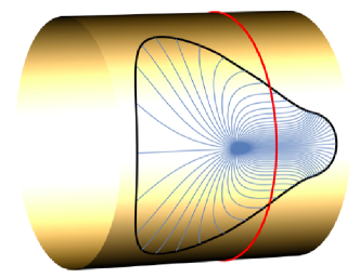
Figure 1: Geodesics on the Grushin cylinder, staring from the point $(-1/2,0)$ with final time $t_{f}=1.3$, crossing smoothly the singular set $Z$ (red circle).

For such a structure, the geodesics cross the singular set $Z=\{(x,y)\in{\bf R}\times S^{1}\mid x=0\}$ without singularities (see Figure 1), while the Riemannian metric $g$, the Riemannian area $\omega$ and the Gaussian curvature $K$ are deeply singular on $Z$:

$$g=\left(\begin{array}[]{cc}1&0\\ 0&1/x^{2}\end{array}\right),~{}~{}~{}\omega=\frac{1}{|x|}dx\,dy,~{}~{}~{}K=-\frac{2}{x^{2}}.$$ (3)

However even if geodesics cross the singular set, this is not possible for the Brownian motion or for a quantum particle when they are described by the Laplace-Beltrami operator $\Delta$ associated to the $2$-ARS. This is due to the explosion of the Riemannian area while approaching $Z$ that makes appearing highly singular first order terms in $\Delta$. For instance for the Grushin cylinder the Laplace-Beltrami operator is given by

$$\Delta={\rm div}_{\omega}\circ{\rm grad}_{g}=\dfrac{\partial^{2}}{\partial x^{2}}+x^{2}\dfrac{\partial^{2}}{\partial y^{2}}-\frac{1}{x}\dfrac{\partial}{\partial x}.$$

This phenomenon is described by the following Theorem.

Theorem 1 ([15]).

Let $M$ be a compact oriented $2$-dimensional manifold equipped with a genuine 2-step $2$-ARS. Let $\Omega$ be a connected component of $M\setminus Z$, where $Z$ is the singular set. Let $g$ be the Riemannian metric induced by the $2$-ARS on $\Omega$ and $\omega$ be the corresponding Riemannian area. The Laplace-Beltrami operator $\Delta:={\rm div}_{\omega}\circ{\rm grad}_{g}$ with domain $C^{\infty}_{0}(\Omega)$, is essentially self-adjoint on $L^{2}(\Omega,\omega)$.

Notice that by construction each connected component of $\partial\Omega$ is diffeomorphic to $S^{1}$, $\Omega$ is open and $(\Omega,g)$ is a non-complete Riemannian manifold. In Theorem 1 the compactness hypothesis is not necessary, but simplifies the statement. In particular the conclusion of the theorem holds for the Grushin cylinder. Versions of Theorem 1 in more general settings have been proved in [23, 35].

The main consequence of Theorem 1 is that the Cauchy problems for the heat and the Schrödinger equations (here $\Delta$ is the Laplace-Beltrami operator, $\hbar$ is the Planck constant, and $m$ is the mass of the quantum particle)

$$\partial_{t}\phi(t,p) = \Delta\,\phi(t,p),~{}~{}~{}~{}~{}~{}~{}~{}~{}~{}~{}~{}~{}~{}\phi(0,\cdot)=\phi_{0}\in L^{2}(\Omega,\omega),$$ (4)

$$\mathrm{i}\hbar\,\partial_{t}\psi(t,p) = -\frac{\hbar^{2}}{2m}\Delta\,\psi(t,p),~{}~{}~{}~{}~{}~{}~{}\psi(0,\cdot)=\psi_{0}\in L^{2}(\Omega,\omega).$$ (5)

are well defined in $L^{2}(\Omega,\omega)$ and hence nothing can flow outside $\Omega$, that is, $e^{t\Delta}\phi_{0}$ (resp. $e^{\mathrm{i}t\frac{\hbar}{2m}\Delta}\psi_{0}$) is supported in $\Omega$, for all $t\geq 0$ (resp. $t\in{\bf R}$). This phenomenon is usually known as quantum confinement (see [23, 35] and, for similar problems, [33]).

Given that the geodesics cross the singular set with no singularities, the impossibility for the heat or for a quantum particle to flow through $Z$ implied by Theorem 1 is quite surprising. For what concerns the heat, a satisfactory interpretation of Theorem 1 in terms of Brownian motion/Bessel processes has been provided for the Grushin cylinder in [16] and from [2] one can extract an interpretation of Theorem 1 in terms of random walks. Roughly speaking random particles are lost in the infinite area accumulated along $Z$ that, as a consequence, acts as a barrier.

Although for the heat-equation the situation is relatively well-understood, this is not the case for the Schrödinger equation since semiclassical analysis (see for instance [41]) roughly says that for $\hbar\to 0$ sufficiently concentrated solutions of the Schrödinger equation move approximately along classical geodesics. Clearly semiclassical analysis breaks down on the singularity $Z$.

It is then natural to come back on the quantization procedure that permits to pass from the description of a free classical particle moving on a Riemannian manifold to the corresponding Schrödinger equation.

This is a complicated subject that has no unique answer. The resulting evolution equation for quantum particles depends indeed on the chosen quantization procedure.

Most of coordinate invariant quantization procedures modify the quantum Hamiltonian by a correction term depending on the scalar curvature $R$. In dimension two, the scalar curvature is twice the Gaussian curvature $K$ and the modified Schrödinger equation is of the form

$$\mathrm{i}\hbar\,\partial_{t}\psi(t,p)=\frac{\hbar^{2}}{2m}\Big{(}-\Delta+cK(p)\Big{)}\psi(t,p),$$

where $c\geq 0$ is a constant. Values given in the literature include:

• path integral quantization: $c=1/3$ and $c=2/3$ in [22], $c=1/2$ in [21];

• covariant Weyl quantization: $c\in[0,2/3]$ including conventional Weyl quantization ($c=0$) in [25];

• geometric quantization for a real polarization: $c=1/3$ in [40];

• finite dimensional approximations to Wiener Measures: $c=2/3$ in [6].

We refer to [6, 25] for interesting discussions on the subject.

Purpose of this paper is to study the self-adjointness of the curvature Laplacian $-\Delta+cK$ depending on $c$ to understand if quantum confinement holds for the dynamics induced by this operator. Before stating our main result, let us remark that the curvature term $cK$ interacts with the diverging first order term in $\Delta$.

For instance for the Grushin cylinder a unitary transformation (see Section 4.1, (22)) permits to transform the operator

$$\Delta=\dfrac{\partial^{2}}{\partial x^{2}}+x^{2}\dfrac{\partial^{2}}{\partial y^{2}}-\frac{1}{x}\dfrac{\partial}{\partial x}\mbox{ on }L^{2}\left({\bf R}\times S^{1},\frac{1}{|x|}dx\,dy\right)$$

in

$$\tilde{\Delta}=\dfrac{\partial^{2}}{\partial x^{2}}+x^{2}\dfrac{\partial^{2}}{\partial y^{2}}-\frac{3}{4}\dfrac{1}{x^{2}}\mbox{ on }L^{2}({\bf R}\times S^{1},dx\,dy)$$

and hence the adding of a term of the form $-cK=-c\big{(}-2\frac{1}{x^{2}}\big{)}$ (that remains untouched by the unitary transformation) to $\tilde{\Delta}$ changes the diverging behaviour around ${x=0}$. In particular for $c=3/8$ the diverging potential disappears and $-\tilde{\Delta}+cK$ is not essentially self-adjoint in $L^{2}({\bf R}_{+}\times S^{1},dx\,dy)$ while $-\tilde{\Delta}$ does. The same conclusion applies to $-\Delta+cK$ in $L^{2}({\bf R}_{+}\times S^{1},\frac{1}{|x|}dx\,dy)$.

The main result of the paper is that the perturbation term given by the curvature destroys the essential self-adjointness of the Laplace-Beltrami operator.

Theorem 2.

Let $M$ be a compact oriented $2$-dimensional manifold equipped with a genuine 2-step $2$-ARS. Let $\Omega$ be a connected component of $M\setminus Z$, where $Z$ is the singular set. Let $g$ be the Riemannian metric induced by the $2$-ARS on $\Omega$, $\omega$ be the corresponding Riemannian area, $K$ the corresponding Gaussian curvature and $\Delta={\rm div}_{\omega}\circ{\rm grad}_{g}$ the Laplace-Beltrami operator. Let $c\in[0,1/2)$. The curvature Laplacian $-\Delta+cK$ with domain $C^{\infty}_{0}(\Omega)$, is essentially self-adjoint on $L^{2}(\Omega,\omega)$ if and only if c=0. Moreover, if $c>0$, the curvature Laplacian has infinite deficiency indices.

The non-self-adjointness of $-\Delta+cK$ implies that one can construct self-adjoint extensions of this operator that permit to the solution to the Schrödinger equation to flow out of the set $\Omega$, in the same spirit of [17, 27]. The study of these self-adjoint extension and how semiclassical analysis applies to them is a subject that deserves to be studied in detail.

Remark 3.

We remark that in Theorem 2 the hypothesis $c\in[0,1/2)$ guarantees the non-negativity of the operator $-\Delta+cK$ modulo a Kato-small perturbation. For further details, see also Remark 7, Lemma 25, and Remark 26

Remark 4.

Notice that in Theorem 2 one can also consider the case $c<0$. In this case, one can prove that the curvature Laplacian is essentially self-adjoint (applying for example the criterion for the self-adjointes of operators of the form $-\Delta+V$ on non-complete Riemannian manifolds, found in [35]). However, if this case admits a physical interpretation is not known to the authors.

As in Theorem 1 the compactness hypothesis is useful to simplify the statement of the theorem. A version without the compactness hypothesis is given here where also the orientability assumption of $M$ is not needed.

Theorem 5.

Let $M$ be a $2$-dimensional manifold equipped with a genuine 2-step $2$-ARS.

Assume that

• the singular set $Z$ is compact;

• the $2$-ARS is geodesically complete.

Let $\Omega$ be a connected component of $M\setminus Z$, and $c\in[0,1/2)$. With the same notations of Theorem 2, the curvature Laplacian $-\Delta+cK$ with domain $C^{\infty}_{0}(\Omega)$, is essentially self-adjoint on $L^{2}(\Omega,\omega)$ if and only if c=0. Moreover, if $c>0$, the curvature Laplacian has infinite deficiency indices.

For the sake of simplicity, we prove Theorem 2 only. Theorem 5 can be proved following the same ideas.

Theorem 5 applies in particular to the Grushin cylinder with curvature Laplacian $-\Delta+cK=-(\partial^{2}_{x}+x^{2}\partial^{2}_{y}-\frac{1}{x}\partial_{x})+\frac{2c}{x^{2}}$. For this case, the fact that the deficiency indices are infinite means that all Fourier components of $-\Delta+cK$ are not self-adjoint.

Notice that under the hypothesis of the theorem, each connected component of $\partial\Omega$ is diffeomorfic to $S^{1}.$ Of course if $c>0$, the manifold does not need to be geodesically complete.

If one removes the 2-step hypothesis the situation is more complicated since tangency points [3, 4] may appear. In presence of tangency points even the essential self-adjointness of the standard Laplace-Beltrami operator (without the term $-cK$) is an open question [15]. Without the $2$-step hypothesis results can indeed be very different. To illustrate this, we study the $\alpha$-Grushin cylinder for which computations can be done explicitly for every value of $c$.

Proposition 6.

Fix $\alpha\in{\bf R}$. On ${\bf R}\times S^{1}$ consider the generalized Riemannian structure for which an orthonormal frame is given by

$$X_{1}(x,y)=\dfrac{\partial}{\partial x},\qquad X_{2}^{(\alpha)}(x,y)=x^{\alpha}\dfrac{\partial}{\partial y},\mbox{ ~{}~{}~{} here }x\in{\bf R},~{}~{}y\in S^{1}.$$

Let $c\geq 0$. On ${\bf R}_{+}\times S^{1}$ the structure is Riemannian with Riemannian area $\frac{1}{|x|^{\alpha}}dx\,dy$. Let $-\Delta_{\alpha}+cK_{\alpha}$ be the curvature Laplacian with domain $C^{\infty}_{0}({\bf R}_{+}\times S^{1})$ acting on $L^{2}({\bf R}_{+}\times S^{1},\frac{1}{|x|^{\alpha}}dx\,dy)$. Denote by

$$\alpha_{c,\pm}=\dfrac{(-2c+1)\pm 2\sqrt{(c-2+\sqrt{3})(c-2-\sqrt{3})}}{4c-1}.$$

$$\bullet \text{ If }0\leq c<1/4, -\Delta_{\alpha}+cK_{\alpha} \text{ is essentially self-adjoint if and only if }\alpha\geq\alpha_{c,+}\text{ or }\alpha\leq\alpha_{c,-};$$

$$\bullet \text{ if }c=1/4, -\Delta_{\alpha}+cK_{\alpha} \text{ is essentially self-adjoint if and only if }\alpha\geq 3;$$

$$\bullet \text{ if }1/4<c\leq 2-\sqrt{3}, -\Delta_{\alpha}+cK_{\alpha} \text{ is essentially self-adjoint if and only if }\alpha_{c,-}\leq\alpha\leq\alpha_{c,+};$$

$$\bullet \text{ if }2-\sqrt{3}<c<2+\sqrt{3}, -\Delta_{\alpha}+cK_{\alpha} \text{ is not essentially self-adjoint }\forall\alpha\in{\bf R};$$

$$\bullet \text{ if }c\geq 2+\sqrt{3}, -\Delta_{\alpha}+cK_{\alpha} \text{ is essentially self-adjoint if and only if }\alpha_{c,-}\leq\alpha\leq\alpha_{c,+}.$$

Figure 2: Regions of the $(\alpha,c)$-parameter space where the operator $-\Delta_{\alpha}+cK_{\alpha}$ is essentially self-adjoint.

The regions where $-\Delta_{\alpha}+cK_{\alpha}$ is essentially self-adjoint are plotted in Figure 2. Note that for some of the quantizations listed earlier, $-\Delta_{\alpha}+cK_{\alpha}$ is essentially self-adjoint for $|\alpha|$ sufficiently big. The $\alpha$-Grushin cylinder is an interesting geometric structure studied in [16, 17, 27]. For $\alpha=0$ it is a flat cylinder, for $\alpha$ positive integer is a $(\alpha+1)$-step $2$-ARS; for $\alpha$ negative it describes a conic-like surface (in particular for $\alpha=-1$ describes a flat two-dimensional cone).

Remark 7.

Notice that for $\alpha=1$ the $\alpha$-Grushin cylinder is the standard Grushin cylinder, for which in Proposition 6 we obtain that $-\Delta_{1}+cK_{1}$, $c\geq 0$, is essentially self-adjoint if and only if $c=0$. This suggests that the hypothesis $c\in[0,1/2)$ of Theorem 2 is technical and that the same result could be extended to the range of values $c\geq 0$.

The proof of Proposition 6, which is instructive since it is simple and presents already some crucial ingredients necessary for the general theory, is given in Section 3.

Structure of the paper. In Section 2 we give the key definition and results for $2$-ARS. In Section 3 we introduce the basic concepts to study the self-adjointness of symmetric operators and give a proof of Proposition 6. The proof of Theorem 2 spans Sections 4 and 5. A local version around a singular region is studied in Section 4, where a description of the closure and adjoint curvature Laplacian operators is given. The main tools needed for our proof are the Hardy inequality, the Kato-Rellich perturbation theorem, the Fourier transform, and Sturm-Liouville theory applied here in the context of 2D operators. We then extend the results on the whole manifold in Section 5.

We conclude this introduction by remarking that while an operator of the form $-\Delta+cK(p)$ is useful to describe a quantum particle in a Riemannian manifold, it is not meaningful in the description of the evolution of the heat. Indeed a heat equation of the form $\partial_{t}\phi=(-\Delta+cK(p))\phi$ would describe the evolution of a random particle on a Riemannian manifold with a rate of killing proportional to the Gaussian curvature.

2 2D almost-Riemannian structures

Definition 8.

Let $M$ be a 2D connected smooth manifold. A $2$-dimensional almost-Riemannian Structure ($2$-ARS) on $M$ is a pair $({\mathbf{U}},f)$ as follows:

• ${\mathbf{U}}$ is an Euclidean bundle over $M$ of rank $2$. We denote each fiber by $U_{q}$, the scalar product on $U_{q}$ by $(\cdot\,|\,\cdot)_{q}$ and the norm of $u\in U_{q}$ as $|u|=\sqrt{(u\,|\,u)_{q}}.$

• $f:{\mathbf{U}}\to TM$ is a smooth map that is a morphism of vector bundles i.e., $f(U_{q})\subseteq T_{q}M$ and $f$ is linear on fibers.

• the distribution $\mathcal{D}=\{f(\sigma)\mid\sigma:M\to{\mathbf{U}}$ smooth section$\}$, is a family of vector fields satisfying the Hörmander condition, i.e., defining $\mathcal{D}_{1}:=\mathcal{D}$, $\mathcal{D}_{i+1}:=\mathcal{D}_{i}+[\mathcal{D}_{1},\mathcal{D}_{i}]$, for $i\geq 1$, there exists $s\in{\bf N}$ such that $\mathcal{D}_{s}(q)=T_{q}M$.

A particular case of 2-ARSs is given by Riemannian surfaces. In this case ${\mathbf{U}}=TM$ and $f$ is the identity.

Let us recall few key definitions and facts. We refer to [1] for more details.

• Let $\mathcal{D}_{p}=\{X(p)\mid X\in\mathcal{D}\}=f(U_{p})\subseteq T_{p}M$. The set of points in $M$ such that $\dim(\mathcal{D}_{p})<2$ is called singular set and it is denoted by $Z$. Since $\mathcal{D}$ satisfies the Hörmander condition, the subspace $\mathcal{D}_{p}$ is nontrivial for every $p$ and $Z$ coincides with the set of points $p$ where $\mathcal{D}$ is one-dimensional. The $2$-ARS is said to be genuine if $Z\neq\emptyset$. The $2$-ARS is said to be $2$-step if for every $p\in M$ we have $\mathcal{D}_{p}+[\mathcal{D},\mathcal{D}]_{p}=T_{p}M$.

• The (almost-Riemannian) norm of a vector $v\in\mathcal{D}_{p}$ is

  $$\|v\|:=\min\{|u|,\,u\in U_{p}\ \text{ s.t. }\ v=f(p,u)\}.$$

• An admissible curve is a Lipschitz curve $\gamma:[0,T]\to M$ such that there exists a measurable and essentially bounded function $u:[0,T]\ni t\mapsto u(t)\in U_{\gamma(t)}$, called control function, such that $\dot{\gamma}(t)=f(\gamma(t),u(t)),$ for a.e. $t\in[0,T]$. Notice there may be more than one control corresponding to the same admissible curve.

• If $\gamma$ is admissible then $t\to\|\dot{\gamma}(t)\|$ is measurable. The (almost-Riemannian) length of an admissible curve $\gamma:[0,T]\to M$ is

  $$\ell(\gamma):=\int_{0}^{T}\|\dot{\gamma}(t)\|dt.$$

• The (almost-Riemannian) distance between two points $p_{0},p_{1}\in M$ is

  $$d(p_{0},p_{1})=\inf\{\ell(\gamma)\,|\,\gamma:[0,T]\to M\text{ admissible},\ \gamma(0)=p_{0},\ \gamma(T)=p_{1}\}.$$

  Thanks to the bracket-generating condition, the Chow-Rashevskii theorem guarantees that $(M,d)$ is a metric space and that the topology induced by $(M,d)$ is equivalent to the manifold topology.

• Given a local trivialization $\Omega\times{\bf R}^{2}$ of ${\mathbf{U}}$, an orthonormal frame for the $2$-ARS on $\Omega$ is the pair of vector fields $\{F_{1},F_{2}\}:=\{f\circ\sigma_{1},f\circ\sigma_{2}\}$ where $\{\sigma_{1},\sigma_{2}\}$ is an orthonormal frame for $(\cdot\,|\,\cdot)_{q}$ on $\Omega\times{\bf R}^{2}$ of ${\mathbf{U}}$. On a local trivialization the map $f$ can be written as $f(p,u)=u_{1}F_{1}(p)+u_{2}F_{2}(p)$. When this can be done globally (i.e., when ${\mathbf{U}}$ is the trivial bundle) we say that the $2$-ARS is free.

  Notice that orthonormal frames in the sense above are orthonormal frames in the Riemannian sense out of the singular set.

• Locally, for a $2$-ARS, it is always possible to find a system of coordinates and an orthonormal frame that in these coordinates has the form

  $$F_{1}(x,y)=\left(\begin{array}[]{c}1\\ 0\end{array}\right),~{}~{}F_{2}(x,y)=\left(\begin{array}[]{c}0\\ {\mathfrak{f}}(x,y)\end{array}\right),$$ (10)

  where ${\mathfrak{f}}:\Omega\to{\bf R}$ is a smooth function. In these coordinates we have that $Z=\{(x,y)\in\Omega\mid{\mathfrak{f}}(x,y)=0\}$. Using this orthonormal frame one immediately gets:

  Proposition 9.

  The $2$-ARS is $2$-step in $\Omega$ if and only if for every $(x,y)\in\Omega$ such that ${\mathfrak{f}}(x,y)=0$, we have $\partial_{x}{\mathfrak{f}}(x,y)\neq 0$.

  Moreover, the implicit function theorem applied to the function ${\mathfrak{f}}$ directly implies:

  Proposition 10.

  If the $2$-ARS is genuine and $2$-step then $Z$ is a closed embedded one dimensional submanifold.

  In particular if $Z$ is compact, each connected component of $Z$ is diffeomorphic to $S^{1}$.

• Out of the singular set $Z$, the structure is Riemannian and the Riemannian metric, the Riemannian area, the Riemannian curvature, and the Laplace-Beltrami operator are easily expressed in the orthonormal frame given by (10):

  $$g_{(x,y)}=\left(\begin{array}[]{cc}1&0\\ 0&\frac{1}{{\mathfrak{f}}(x,y)^{2}}\end{array}\right),$$ (13)

  $$\omega_{(x,y)}=\frac{1}{|{\mathfrak{f}}(x,y)|}dx\,dy,$$ (14)

  $$K(x,y)=\frac{{\mathfrak{f}}(x,y)\partial_{x}^{2}{\mathfrak{f}}(x,y)-2\left(\partial_{x}{\mathfrak{f}}(x,y)\right)^{2}}{{\mathfrak{f}}(x,y)^{2}},$$ (15)

  $$\Delta=\partial_{x}^{2}+{\mathfrak{f}}^{2}\partial_{y}^{2}-\frac{\partial_{x}{\mathfrak{f}}}{{\mathfrak{f}}}\partial_{x}+{\mathfrak{f}}(\partial_{y}{\mathfrak{f}})\partial_{y}.$$ (16)

• To prove the main results of this paper, the following normal forms are going to be important.

  Proposition 11 ([3]).

  Consider a $2$-step $2$-ARS. For every $p\in M$ there exist a neighborhood $U$ of $p$, a system of coordinates in $U$, and an orthonormal frame $\{X_{1},X_{2}\}$ for the ARS on $U$, such that $p=(0,0)$ and $\{X_{1},X_{2}\}$ has one of the following forms:

  1. $X_{1}(x,y)=\dfrac{\partial}{\partial x},\qquad X_{2}(x,y)=e^{\phi(x,y)}\dfrac{\partial}{\partial y},$

  2. $X_{1}(x,y)=\dfrac{\partial}{\partial x},\qquad X_{2}(x,y)=xe^{\phi(x,y)}\dfrac{\partial}{\partial y},$

  where $\phi$ is a smooth function such that $\phi(0,y)=0$.

  A point $p\in M$ is said to be a Riemannian point if $\mathcal{D}_{p}$ is two-dimensional, and hence a local description around $p$ is given by F1. A point $p$ such that $\mathcal{D}_{p}$ is one-dimensional, and thus $\mathcal{D}_{p}+[\mathcal{D},\mathcal{D}]_{p}$ is two-dimensional, is called a Grushin point and a local description around $p$ is given by F2.

  When $M$ is compact orientable, each connected component of $Z$ is diffeomorphic to $S^{1}$ and admits a tubular neighborhood diffeomorphic to ${\bf R}\times S^{1}$. In this case the normal form F2 can be extended to the whole neighborhood.

  Proposition 12 ([15]).

  Consider a $2$-step $2$-ARS on a compact orientable manifold. Let $W$ be a connected component of $Z$. Then there exist a tubular neighborhood $U$ of $W$ diffeomorphic to ${\bf R}\times S^{1}$, a system of coordinates in $U$, and an orthonormal frame $\{X_{1},X_{2}\}$ of the 2-ARS on $U$ such that $W=\{(0,y),~{}y\in S^{1}\}$ and $\{X_{1},X_{2}\}$ has the form

  $$X_{1}(x,y)=\dfrac{\partial}{\partial x},\qquad X_{2}(x,y)=xe^{\phi(x,y)}\dfrac{\partial}{\partial y}.$$ (17)

3 Self-adjointness of operators

Let $A$ be a linear operator on a separable Hilbert space $\mathcal{H}$, $(\cdot,\cdot)_{\mathcal{H}}$. The linear subspace of $\mathcal{H}$ where the action of $A$ is well-defined is called the domain of $A$, denoted by $\mathcal{D}(A)$. We shall always assume that $\mathcal{D}(A)$ is dense in $\mathcal{H}$. Following [36], we recall several definitions and properties of linear operators:

• $A$ is said to be symmetric if $(Au,v)_{\mathcal{H}}=(u,Av)_{\mathcal{H}}$ for all $u,v\in\mathcal{D}(A)$.

• $A$ is said to be closed if $\mathcal{D}(A)$ with the norm $\|\cdot\|_{A}:=\|\cdot\|_{\mathcal{H}}+\|A\cdot\|_{\mathcal{H}}$ is complete.

• A linear operator $B$, $\mathcal{D}(B)$ such that $\mathcal{D}(A)\subset\mathcal{D}(B)$ and $Bu=Au$ for all $u\in\mathcal{D}(A)$ is called an extension of $A$. In this case we write $A\subset B$.

• If $A$ is symmetric and densely defined, there exists a minimal closed symmetric extension $\overline{A}$ of $A$, which is said to be the closure of $A$. We describe this construction: take any sequence $(u_{n})_{n}\subset\mathcal{D}(A)$ which converges to a limit $u\in\mathcal{H}$, and for which the sequence $(Au_{n})_{n}$ converges to a limit $w\in\mathcal{H}$. Then, by symmetry of $A$, we have that

  $$(w,v)_{\mathcal{H}}=\lim_{n\to\infty}(Au_{n},v)_{\mathcal{H}}=\lim_{n\to\infty}(u_{n},Av)_{\mathcal{H}}=(u,Av)_{\mathcal{H}},\quad\forall v\in\mathcal{D}(A).$$

  Since $\mathcal{D}(A)$ is dense in $\mathcal{H}$, $w$ is uniquely determined by $u$. The closure of $A$ is defined by setting $\overline{A}u=w$, and the domain $\mathcal{D}(\overline{A})$ is the closure of $\mathcal{D}(A)$ with respect to the norm $\|\cdot\|_{A}$. One can easily see that $\overline{A}$ is closed, symmetric, and any closed extension of $A$ is an extension of $\overline{A}$ as well.

• Given a densely defined linear operator $A$, the domain $\mathcal{D}(A^{*})$ of the adjoint operator $A^{*}$ is the set of all $v\in\mathcal{H}$ such that there exists $w\in\mathcal{H}$ with $(Au,v)_{\mathcal{H}}=(u,w)_{\mathcal{H}}$ for all $u\in\mathcal{D}(A)$. The adjoint of $A$ is defined by setting $A^{*}v=w$.

• $A$ is said to be self-adjoint if $A^{*}=A$, that is, $A$ is symmetric and $\mathcal{D}(A^{*})=\mathcal{D}(A)$.

• $A$ is said to be essentially self-adjoint if its closure is self-adjoint.

• If $B$ is a closed symmetric extension of $A$, then $A\subset\overline{A}\subset B\subset A^{*}$.

• If a densely defined operator $B$ is such that $\mathcal{D}(A)\subset\mathcal{D}(B)$ and there exist $a,b\geq 0$ such that

  $$\|Bu\|\leq a\|Au\|+b\|u\|,\qquad\forall u\in\mathcal{D}(A),$$ (18)

  then $B$ is said to be small with respect to $A$ (or also, Kato-small w.r.t. $A$). The infimum of the set of $a\geq 0$ such that (18) holds is called the $A$-bound of $B$. If $a$ can be chose arbitrarily small, $B$ is said to be infinitesimally small w.r.t $A$.

We will need the following classical result in perturbation theory:

Proposition 13 (Kato-Rellich’s Theorem).

Let $A,B$ be two densely defined operators and assume that $B$ is small with respect to $A$. Then $D(\overline{A})\subset D(\overline{A+B})$. If moreover $a<1$ in (18), then $D(\overline{A})=D(\overline{A+B})$.

In order to study the self-adjointness and more in general describe the extensions of a symmetric operator $A$, one may use the fundamental Von Neumann decomposition ([36, Chapter X])

$$\mathcal{D}(A^{*})=\mathcal{D}(\overline{A})\oplus_{A}\ker(A^{*}+\mathrm{i})\oplus_{A}\ker(A^{*}-\mathrm{i}),$$ (19)

where the sum is orthogonal with respect to the scalar product $(\cdot,\cdot)_{A}=(\cdot,\cdot)_{\mathcal{H}}+(A^{*}\cdot,A^{*}\cdot)_{\mathcal{H}}.$ As a first direct consequence of (19), one has the fundamental spectral criterion for self-adjointness:

Proposition 14.

Let $A$, $\mathcal{D}(A)$, be a symmetric operator, densely defined on the Hilbert space $\mathcal{H}$. The following are equivalent:

1. $A$ is essentially self-adjoint;

2. $\mathrm{Ran}(A\pm\mathrm{i})$ is dense in $\mathcal{H}$;

3. $\ker(A^{*}\pm\mathrm{i})=\{0\}$.

• The dimensions of the vector spaces $\ker(A^{*}+\mathrm{i})$ and $\ker(A^{*}-\mathrm{i})$ are called deficiency indices of $A$.

Always using (19), one can deduce that $A$ admits self-adjoint extensions if and only if its deficiency indices are equal ([36, Corollary to Theorem X.2]).

Another immediate consequence of (19) is the following fact concerning 1D operators: let $A$ be a 1D Sturm-Liouville operator $-\frac{d^{2}}{dx^{2}}+V(x)$, where $V$ is a continuous real function on ${\bf R}_{+}$, acting on $L^{2}({\bf R}_{+},dx)$ with domain $C^{\infty}_{0}({\bf R}_{+})$ (for a general introduction to 1D Sturm-Liouville operators, see e.g. [37, Chapter 15]). Then, since the eigenvalue equation

$$-u^{\prime\prime}(x)+V(x)u(x)=\pm\mathrm{i}\,u(x)$$

has always two linearly independent solutions, the quotient $\mathcal{D}(A^{*})/\mathcal{D}(\overline{A})$ has at most dimension four. Moreover, let us recall the limit point-limit circle Weyl’s Theorem (see, e.g, [36, Appendix to Chapter X.1]) which says that the self-adjointness of a 1D Sturm-Liouville operator can be deduced by regarding the solutions to the ODE

$$-u^{\prime\prime}(x)+V(x)u(x)=0.$$ (20)

• If all solutions to (20) are square-integrable near $0$ (respectively $\infty$), then $V$ is said to be in the limit circle case at $0$ (resp. $\infty$). If $V$ is not in the limit circle case at $0$ (resp. $\infty$), it is said to be in the limit point case at $0$ (resp. $\infty$).

Proposition 15 (Weyl’s Theorem).

The operator $-\frac{d^{2}}{dx^{2}}+V(x)$ with domain $C^{\infty}_{0}({\bf R}_{+})$ has deficiency indices

• $(2,2)$ if $V$ is in the limit circle case at both $0$ and $\infty$;

• $(1,1)$ if $V$ is in the limit circle case at one end point and in the limit point at the other;

• $(0,0)$ if $V$ is in the limit point case at both $0$ and $\infty$.

In particular, $-\frac{d^{2}}{dx^{2}}+V(x)$ is essentially self-adjoint on $L^{2}({\bf R}_{+},dx)$ if and only if $V$ is in the limit point case at both $0$ and $\infty$.

Some useful criteria to determine whether a potential $V$ is in the limit point or limit circle case (it is also said to be quantum-mechanically complete or incomplete, respectively) at $0$ and $\infty$ are the following:

Proposition 16.

Let $V\in C^{1}({\bf R}_{+})$ be real and bounded above by a constant $E$ on $[1,\infty)$. Suppose that $\int_{1}^{\infty}\frac{1}{\sqrt{E-V(x)}}dx=\infty$ and $V^{\prime}/|V|^{3/2}$ is bounded near $\infty$. Then $V$ is in the limit point case at $\infty$.

Proposition 17.

Let $V\in C^{0}({\bf R}_{+})$ be real and positive near $0$. If $V(x)\geq\frac{3}{4x^{2}}$ near $0$ then $V$ is in the limit point case at $0$. If for some $\epsilon>0$, $V(x)\leq(\frac{3}{4}-\epsilon)\frac{1}{x^{2}}$ near $0$, then $V$ is in the limit circle case at $0$.

Proposition 18.

Let $V\in C^{0}({\bf R}_{+})$ be real, and suppose that it decreases as $x\downarrow 0$. Then $V$ is in the limit circle case at $0$.

Weyl’s Theorem and these criteria are, respectively, [36, Theorem X.7, Corollary to Theorem X.8, Theorem X.10 and Problem X.7 ].

Here we give the proof of Proposition 6, which makes use of the limit point-limit circle argument.

Proof.

of Proposition 6   The Laplace-Beltrami operator (with domain $C^{\infty}_{0}({\bf R}_{+}\times S^{1})$) and the curvature associated to the orthonormal frame $X_{1},X_{2}^{(\alpha)}$ are given by

$$\Delta_{\alpha}=\frac{\partial^{2}}{\partial x^{2}}+x^{2\alpha}\frac{\partial^{2}}{\partial y^{2}}-\frac{\alpha}{x}\frac{\partial}{\partial x},\quad K_{\alpha}=-\frac{\alpha(\alpha+1)}{x^{2}}.$$

We perform a unitary transformation

$$U_{\alpha}:L^{2}\Big{(}{\bf R}_{+}\times S^{1},\frac{1}{|x|^{\alpha}}dx\,dy\Big{)}\rightarrow L^{2}({\bf R}_{+}\times S^{1},dx\,dy),\quad\psi\mapsto|x|^{-\alpha/2}\psi,$$

which gives the operator

$$L_{\alpha,c}:=U_{\alpha}(-\Delta_{\alpha}+cK_{\alpha})U_{\alpha}^{-1}=-\frac{\partial^{2}}{\partial x^{2}}-x^{2\alpha}\frac{\partial^{2}}{\partial y^{2}}+\frac{(1-4c)\alpha^{2}+(2-4c)\alpha}{4x^{2}}.$$

Via Fourier transform with respect to the variable $y\in S^{1}$, one obtains the direct sum operator

$$\widetilde{L}_{\alpha,c}:=\bigoplus_{k\in{\bf Z}}(L_{\alpha,c})_{k},\quad(L_{\alpha,c})_{k}:=-\frac{\partial^{2}}{\partial x^{2}}+x^{2\alpha}k^{2}+\frac{(1-4c)\alpha^{2}+(2-4c)\alpha}{4x^{2}},$$

acting on the Hilbert space $\ell^{2}(L^{2}({\bf R}_{+}))$, with domain $\mathcal{D}(\widetilde{L}_{\alpha,c})=\{(f_{k})_{k\in{\bf Z}}\in\ell^{2}(L^{2}({\bf R}_{+}))\mid f_{k}\in\mathcal{D}((L_{\alpha,c})_{k})\;\forall k\in{\bf Z},f_{k}=0\text{ for almost every $k$}\}$, where $\mathcal{D}\Big{(}(L_{\alpha,c})_{k}\Big{)}=C^{\infty}_{0}({\bf R}_{+})$ for all $k$. Moreover, as a general fact concerning direct sum operators, $\widetilde{L}_{\alpha,c}$ is essentially self-adjoint if and only if $(L_{\alpha,c})_{k}$ is so for all $k$ ([17, Proposition 2.3]). Let us thus study the essential self-adjointness of $(L_{\alpha,c})_{0}$: it is a Sturm-Liouville operator of the form $-\frac{d^{2}}{dx^{2}}+V_{\alpha,c}(x)$, where

$$V_{\alpha,c}(x)=\frac{(1-4c)\alpha^{2}+(2-4c)\alpha}{4x^{2}}=:\frac{k(\alpha,c)}{x^{2}}.$$ (21)

The potential $V_{\alpha,c}$ is quantum-mechanically complete at infinity, for all $(\alpha,c)\in{\bf R}\times[0,\infty)$ (as one can check by applying Proposition 16). So, applying Propositions 17 and 18, we can conclude that $2(L_{\alpha,c})_{0}$ is essentially self-adjoint if and only if $V_{\alpha,c}(x)\geq\frac{3}{4x^{2}}$ near zero, since $V_{\alpha,c}(x)=k(\alpha,c)/x^{2}$ and when $k(\alpha,c)<0$ then $V_{\alpha,c}$ decreases for $x\downarrow 0$. By using the explicit formula (21) for $V_{\alpha,c}$, we obtain $k(\alpha,c)\geq 3/4$ which yields the values of $(\alpha,c)$ given in the statement. For what we said before, when $(L_{\alpha,c})_{0}$ is not essentially self-adjoint, neither is so $\widetilde{L}_{\alpha,c}$. Finally, when $(L_{\alpha,c})_{0}$ is essentially self-adjoint, then

$$x^{2\alpha}k^{2}+\frac{(1-4c)\alpha^{2}+(2-4c)\alpha}{4x^{2}}\geq\frac{3}{4x^{2}},$$

so $(L_{\alpha,c})_{k}$ is essentially self-adjoint too, for all $k$, and hence $\widetilde{L}_{\alpha,c}$ is so. $\Box$∎

Remark 19.

As a by-product of the proof of Proposition 6 we obtain that for the Grushin cylinder ($\alpha=1$) with $c>0$ all Fourier components of $-\Delta_{1}+cK_{1}$ are not essentially self-adjoint, due to the inequality $x^{2}k^{2}+(\frac{3}{4}-2c)\frac{1}{x^{2}}<\frac{3}{4x^{2}}$ which holds near zero for all $k\in{\bf Z}$. Hence $-\Delta_{1}+cK_{1}$ has infinite deficiency indices, for any $c>0$. When $c\in(0,1/2)$, Theorem 2 extends this result to any two-dimensional almost Riemannian manifold of step $2$ (under some natural topological assumptions).

However, from this proof we can also point out that this is not always the case for the $\alpha$-Grushin cylinder, as for instance in the case of a flat cone ($\alpha=-1$) with $c\geq 0$ (note that this is not an ARS). In that case, the inequality $(k^{2}-\frac{1}{4})\frac{1}{x^{2}}\geq\frac{3}{4x^{2}}$ implies that the $k$-th’s Fourier components of $-\Delta_{-1}+cK_{-1}$ are essentially self-adjoint for all $k\neq 0$, even if $(-\Delta_{-1}+cK_{-1})_{0}$ is not. This means that $-\Delta_{-1}+cK_{-1}$ has deficiency indices equal to $1$, for all $c\geq 0$.

We conclude this Section by considering a Riemannian manifold $(M,g)$ without boundary, with associated Riemannian volume form $\omega$, and Laplace-Beltrami operator $\Delta={\rm div}_{\omega}\circ{\rm grad}_{g}$ acting on the Hilbert space $L^{2}(M,\omega)$, with domain $\mathcal{D}(\Delta)=C^{\infty}_{0}(M)$. Green’s identity implies

1. $\int_{M}\overline{u}\;\Delta v\;d\omega=\int_{M}\overline{\Delta u}\;v\;d\omega$, for all $u,v\in C^{\infty}_{0}(M)$, i.e., $\Delta$ is a symmetric operator.

2. $\mathcal{D}(\Delta^{*})=\{u\in L^{2}(M,\omega)\mid\Delta u\in L^{2}(M,\omega)\text{ in the sense of distributions}\}.$

Letting $F$ be a real-valued continuous function locally $L^{2}(M,\omega)$ seen as a multiplicative operator with domain $C^{\infty}_{0}(M)$, (i) and (ii) still hold true for the operator $\Delta+F$ instead of $\Delta$.

Remark 20.

Being $\Delta+F$ a real operator (that is, it commutes with complex conjugation), its deficiency indices are equal ([36, Theorem X.3]) and thus it always admits self-adjoint extensions.

4 Grushin zone

We focus now our attention around a Grushin point. We thus define the Riemannian manifold $\Omega=\{(x,y)\in{\bf R}\times S^{1}\mid x\neq 0\}$ with metric $g=\mathrm{diag}(1,x^{-2}e^{-2\phi(x,y)})$, where $\phi$ is a smooth function which is constant for large $|x|$ . The smoothness of $\phi$ is guaranteed by Proposition 11, and even if it is only defined locally, we extend it constantly in the coordinates $(x,y)$, since what matters is the analysis close to $x=0$. Note that $X_{1},X_{2}$ given by Proposition 11 (F2) is an orthonormal frame for $g$. We then consider also the two connected components $\Omega_{+}=\{(x,y)\in{\bf R}\times S^{1}\mid x>0\}$ and $\Omega_{-}=\{(x,y)\in{\bf R}\times S^{1}\mid x<0\}$. We start by proving the following key result:

Theorem 21.

Consider the Riemannian manifold $(\Omega_{+},g)$, with associated Riemannian volume form $\omega$, curvature $K$ and Laplace-Beltrami operator $\Delta$. Let $c\in(0,1/2)$. Consider the curvature Laplacian $-\Delta+cK$, with domain $C_{0}^{\infty}(\Omega_{+})$, acting on $L^{2}(\Omega_{+},\omega)$. Then for every $\epsilon>0$ there exist functions $h_{\pm,\epsilon,c}\in L^{2}(\Omega_{+},\omega)\cap C^{\infty}(\Omega_{+})$ such that

1. $h_{\pm,\epsilon,c}\in\mathcal{D}((-\Delta+cK)^{*})$;

2. $h_{\pm,\epsilon,c}\notin\mathcal{D}(\overline{-\Delta+cK})$;

3. $\mathrm{supp}(h_{\pm,\epsilon,c})\subset(0,\epsilon)\times S^{1}$.

In particular, $-\Delta+cK$ is not essentially self-adjoint (here $c\neq 0$). The same conclusions hold if we replace $\Omega_{+}$ with $\Omega_{-}$ or $\Omega$.

What we can actually prove is the following stronger version of Theorem 21:

Theorem 22.

With the same assumptions and notations of Theorem 21, $\dim\mathcal{D}((-\Delta+cK)^{*})/\mathcal{D}(\overline{-\Delta+cK})=\infty$, i.e., $-\Delta+cK$ has infinite deficiency indices.

The proofs of Theorems 21 and 22 span Sections 4.1 and 4.2, where we shall describe respectively the closure and the adjoint of $-\Delta+cK$.

4.1 Closure operator

We shall work on the manifold $\Omega_{+}$, being the case $\Omega_{-}$ analogous. Then the statement for $\Omega$ follows from the decomposition $L^{2}(\Omega,\omega)=L^{2}(\Omega_{-},\omega)\oplus^{\perp}L^{2}(\Omega_{+},\omega)$.

For a metric $g$ of the form $\mathrm{diag}(1,{\mathfrak{f}}(x,y)^{-2})$, plugging ${\mathfrak{f}}(x,y)=xe^{\phi(x,y)}$ into (14), (15), and (16) one has the following:

$$\begin{split}&\omega_{(x,y)}=\dfrac{1}{xe^{\phi(x,y)}}dxdy,\\ &K(x,y)=-\dfrac{2}{x^{2}}-\dfrac{2\partial_{x}\phi(x,y)}{x}+\partial_{x}^{2}\phi(x,y)-(\partial_{x}\phi(x,y))^{2},\\ &\Delta=\partial_{x}^{2}+x^{2}e^{2\phi(x,y)}\partial_{y}^{2}-\dfrac{1}{x}\partial_{x}-\partial_{x}\phi(x,y)\partial_{x}+\partial_{y}\phi(x,y)x^{2}e^{2\phi(x,y)}\partial_{y}.\end{split}$$

We perform a unitary transformation

$$U:L^{2}(\Omega_{+},\omega)\rightarrow L^{2}(\Omega_{+},dxdy),\quad\psi\mapsto(xe^{\phi})^{-1/2}\psi,$$ (22)

and the corresponding transformed Laplacian is given by

$$\begin{split}L&=U\Delta U^{-1}\\ &=\partial_{x}^{2}+x^{2}e^{2\phi}\partial_{y}^{2}+2x^{2}e^{2\phi}(\partial_{y}\phi)\partial_{y}-\dfrac{3}{4x^{2}}-\dfrac{\partial_{x}\phi}{2x}-\dfrac{1}{4}(\partial_{x}\phi)^{2}+\dfrac{1}{2}\partial_{x}^{2}\phi+\dfrac{3}{4}x^{2}(\partial_{y}\phi)^{2}e^{2\phi}+\dfrac{1}{2}x^{2}(\partial^{2}_{y}\phi)e^{2\phi}.\end{split}$$

We shall analyze the self-adjointness of the operator

$$-L+cK =U(-\Delta+cK)U^{-1}$$

$$=-\partial_{x}^{2}-x^{2}e^{2\phi}\partial_{y}^{2}-2x^{2}e^{2\phi}(\partial_{y}\phi)\partial_{y}+\Big{(}\dfrac{3}{4}-2c\Big{)}\dfrac{1}{x^{2}}+\dfrac{1-4c}{2}\dfrac{\partial_{x}\phi}{x}+\Big{(}\dfrac{1}{4}-c\Big{)}(\partial_{x}\phi)^{2}$$

$$+\Big{(}c-\dfrac{1}{2}\Big{)}\partial_{x}^{2}\phi-\dfrac{3}{4}x^{2}(\partial_{y}\phi)^{2}e^{2\phi}-\dfrac{1}{2}x^{2}(\partial^{2}_{y}\phi)e^{2\phi}$$

$$=H_{c}+\eta_{c},$$ (23)

where we have defined the operator

$$H_{c}=-\partial_{x}^{2}-x^{2}e^{2\phi}\partial_{y}^{2}-2x^{2}e^{2\phi}(\partial_{y}\phi)\partial_{y}+\Big{(}\dfrac{3}{4}-2c\Big{)}\dfrac{1}{x^{2}}+\Big{(}\dfrac{1-4c}{2}\Big{)}\dfrac{\partial_{x}\phi}{x},$$

and the multiplicative operator

$$\eta_{c}=\Big{(}\dfrac{1}{4}-c\Big{)}(\partial_{x}\phi)^{2}+\Big{(}c-\dfrac{1}{2}\Big{)}\partial_{x}^{2}\phi-\dfrac{3}{4}x^{2}(\partial_{y}\phi)^{2}e^{2\phi}-\dfrac{1}{2}x^{2}(\partial^{2}_{y}\phi)e^{2\phi},$$

both with domain $C_{0}^{\infty}(\Omega_{+})$, acting on the Hilbert space $L^{2}(\Omega_{+},dxdy)=:L^{2}(\Omega_{+})$. For later convenience, we also define the operator

$$T_{c}=-\partial_{x}^{2}-x^{2}e^{2\phi}\partial_{y}^{2}-2x^{2}e^{2\phi}(\partial_{y}\phi)\partial_{y}+\Big{(}\dfrac{3}{4}-2c\Big{)}\dfrac{1}{x^{2}},\quad\mathcal{D}(T_{c})=C^{\infty}_{0}(\Omega_{+}),\quad\text{acting on }L^{2}(\Omega_{+}),$$

and the 1D operator, usually called inverse square potential or Bessel operator in the literature

$$s_{c}=-\dfrac{d^{2}}{dx^{2}}+\Big{(}\frac{3}{4}-2c\Big{)}\dfrac{1}{x^{2}},\quad\mathcal{D}(s_{c})=C^{\infty}_{0}({\bf R}_{+}),\quad\text{acting on }L^{2}({\bf R}_{+}).$$ (24)

The closure of $s_{c}$ is known:

Proposition 23.

([5, Theorem 5.1 (ii)]) Let $c\in(0,1/2]$. Then, $\mathcal{D}(\overline{s_{c}})=H^{2}_{0}({\bf R}_{+})$.

Remark 24.

The assumption $c\in(0,1/2]$ in Proposition 23 guarantees that $s_{c}$ is a non-negative operator. Anyway, in the recent paper [19] it is proved that $\mathcal{D}(\overline{s_{c}})=H^{2}_{0}({\bf R}_{+})$ for all $c>0$.

Lemma 25.

Let $c\in[0,1/2)$ and $f\in L^{2}(\Omega_{+})$ with ${\rm supp}f\subset(0,\epsilon)\times S^{1}$, for some $\epsilon>0$. Then, $f\in\mathcal{D}\left(\overline{-L+cK}\right)$ if and only if $f\in\mathcal{D}(\overline{T_{c}})$.

Proof.

Since $-L+cK=H_{c}+\eta_{c}$, and $\eta_{c}$ is a bounded operator on $(0,\epsilon)\times S^{1}$, Proposition 13 implies that $f\in\mathcal{D}(\overline{-L+cK})$ if and only if $f\in\mathcal{D}(\overline{H_{c}})$, for all $c>0$. Furthermore, we want to show that the singular term $\frac{g_{1,c}}{x}:=\left(\frac{1-4c}{2}\right)\frac{\partial_{x}\phi}{x}$ is infinitesimally small w.r.t. $T_{c}$, if $c\in[0,1/2)$. In order to do this we will use two main ingredients. The first one is Hardy inequality:

$$\int_{0}^{\infty}\frac{|f(x)|^{2}}{x^{2}}dx\leq 4\int_{0}^{\infty}|f^{\prime}(x)|^{2}dx\quad\forall f\in C^{\infty}_{0}({\bf R}_{+}).$$

The second one is perturbation theory, in particular Kato-Rellich’s Theorem (Proposition 13).

For all functions $f\in C_{0}^{\infty}({\bf R}_{+}\times S^{1})$ we have

$$\left\|\frac{g_{1,c}f}{x}\right\|^{2}_{L^{2}({\bf R}_{+}\times S^{1})}=\int_{{\bf R}_{+}\times S^{1}}\frac{|g_{1,c}(x,y)|^{2}}{x^{2}}|f(x,y)|^{2}dxdy$$

$$= \left(1-\frac{3-8c}{4-8c}\right)\int_{{\bf R}_{+}\times S^{1}}|g_{1,c}(x,y)|^{2}\frac{|f(x,y)|^{2}}{x^{2}}dxdy+\frac{3-8c}{4-8c}\int_{{\bf R}_{+}\times S^{1}}|g_{1,c}(x,y)|^{2}\frac{|f(x,y)|^{2}}{x^{2}}dxdy$$

$$\leq \||g_{1,c}|^{2}\|_{L^{\infty}({\bf R}_{+}\times S^{1})}\left(\frac{4}{4-8c}\int_{{\bf R}_{+}\times S^{1}}|\partial_{x}f(x,y)|^{2}dxdy+\frac{3-8c}{4-8c}\int_{{\bf R}_{+}\times S^{1}}\frac{|f(x,y)|^{2}}{x^{2}}dxdy\right)$$

$$\leq \frac{4\||g_{1,c}|^{2}\|_{L^{\infty}({\bf R}_{+}\times S^{1})}}{4-8c}\left(\int_{{\bf R}_{+}\times S^{1}}|\partial_{x}f(x,y)|^{2}+x^{2}e^{2\phi}|\partial_{y}f(x,y)|^{2}+\left(\frac{3}{4}-2c\right)\frac{|f(x,y)|^{2}}{x^{2}}dxdy\right)$$

$$= \frac{4\||g_{1,c}|^{2}\|_{L^{\infty}({\bf R}_{+}\times S^{1})}}{4-8c}(T_{c}f,f)_{L^{2}({\bf R}_{+}\times S^{1})}$$

$$\leq \frac{2\||g_{1,c}|^{2}\|_{L^{\infty}({\bf R}_{+}\times S^{1})}}{4-8c}\left(\delta\|T_{c}f\|^{2}_{L^{2}({\bf R}_{+}\times S^{1})}+\frac{1}{\delta}\|f\|^{2}_{L^{2}({\bf R}_{+}\times S^{1})}\right),$$

where we have used Fubini’s Theorem and the Hardy inequality in the first inequality, we have integrated by parts in the third equality, and we have used the Young inequality in the last inequality that holds for every $\delta>0$. This proves that $\frac{g_{1,c}}{x}$ is infinitesimally small w.r.t. $T_{c}$ if $c\in[0,1/2)$. Proposition 13 then implies that $D(\overline{H_{c}})=D(\overline{T_{c}})$ if $c\in[0,1/2)$. $\Box$∎

Remark 26.

The assumption $c\in(0,1/2)$ is used in the proof of Lemma 25 to guarantee the non-negativity of $T_{c}$.

For any function $f\in L^{2}({\bf R}_{+}\times S^{1})$, we denote by $f=\sum_{k\in{\bf Z}}\widehat{f}_{k}(x)e^{\mathrm{i}ky}$ its Fourier series.

Lemma 27.

Let $c\in(0,1/2)$, and let $f\in\mathcal{D}(\overline{-L+cK})$ be a function supported in $(0,\epsilon)\times S^{1}$, for some $\epsilon>0$. Then, $\widehat{f}_{k}(x)=o(x^{\frac{3}{2}})$ as $x\rightarrow 0^{+}$, for every $k\in{\bf Z}$.

Proof.

Let $f\in C^{\infty}_{0}((0,\epsilon)\times S^{1})$. Lemma 25 shows that $f\in\mathcal{D}(\overline{-L+cK})$ if and only if $f\in\mathcal{D}(\overline{T_{c}})$. Thus, we are left to study the behavior near $x=0$ of a function $f\in\mathcal{D}(\overline{T_{c}})$. For any $k\in{\bf Z}$, we have

$$\widehat{(T_{c}\;f)}_{k}=s_{c}\widehat{f}_{k}-\frac{1}{2}x^{2}\sum_{m+m^{\prime}=k}(-m^{2})\widehat{f}_{m}\widehat{(e^{2\phi})}_{m^{\prime}}-x^{2}\sum_{m+m^{\prime}=k}(\mathrm{i}m)\widehat{f}_{m}\widehat{(\partial_{y}\phi\,e^{2\phi})}_{m^{\prime}},$$

where $s_{c}$ is defined in (24), and we compute the norm using the triangular inequality

$$\|\widehat{(T_{c}\;f)}_{k}\|_{L^{2}({\bf R}_{+})}\geq\Big{\|}s_{c}\widehat{f}_{k}\Big{\|}_{L^{2}({\bf R}_{+})}$$

$$- \Big{\|}\frac{1}{2}x^{2}\sum_{m+m^{\prime}=k}(-m^{2})\widehat{f}_{m}\widehat{(e^{2\phi})}_{m^{\prime}}\Big{\|}_{L^{2}({\bf R}_{+})}-\Big{\|}x^{2}\sum_{m+m^{\prime}=k}(\mathrm{i}m)\widehat{f}_{m}\widehat{(\partial_{y}\phi\,e^{2\phi})}_{m^{\prime}}\Big{\|}_{L^{2}({\bf R}_{+})}.$$

We have,

$$\begin{split}&\Big{\|}\sum_{m+m^{\prime}=k}(-m^{2})\widehat{f}_{m}\widehat{(e^{2\phi})}_{m^{\prime}}\Big{\|}_{L^{2}({\bf R}_{+})}\\ =&\Big{\|}\sum_{m+m^{\prime}=k}(-m^{\prime 2})\widehat{f}_{m}\widehat{(e^{2\phi})}_{m^{\prime}}-k^{2}\sum_{m+m^{\prime}=k}\widehat{f}_{m}\widehat{(e^{2\phi})}_{m^{\prime}}+2k\sum_{m+m^{\prime}=k}m^{\prime}\widehat{f}_{m}\widehat{(e^{2\phi})}_{m^{\prime}}\Big{\|}_{L^{2}({\bf R}_{+})}\\ \leq&\|f\|_{L^{2}({\bf R}_{+}\times S^{1})}\Big{(}\sup_{x\in{\bf R}_{+}}\|e^{2\phi}\|_{H^{2}(S^{1})}+k^{2}\sup_{x\in{\bf R}_{+}}\|e^{2\phi}\|_{L^{2}(S^{1})}+2|k|\sup_{x\in{\bf R}_{+}}\|e^{2\phi}\|_{H^{1}(S^{1})}\;\Big{)}\\ \leq&C_{\phi,k}\;\|f\|_{L^{2}({\bf R}_{+}\times S^{1})}\end{split}$$

thanks to the Cauchy-Schwartz inequality and the Plancherel formula. Similarly,

$$\Big{\|}\sum_{m+m^{\prime}=k}(\mathrm{i}m)\widehat{f}_{m}\widehat{(\partial_{y}\phi\,e^{2\phi})}_{m^{\prime}}\Big{\|}_{L^{2}({\bf R}_{+})}\leq$$

$$\|f\|_{L^{2}({\bf R}_{+}\times S^{1})}\Big{(}\sup_{x\in{\bf R}_{+}}\|e^{2\phi}\partial_{y}\phi\|_{H^{1}(S^{1})}+|k|\sup_{x\in{\bf R}_{+}}\|e^{2\phi}\partial_{y}\phi\|_{L^{2}(S^{1})}\;\Big{)}\leq C^{\prime}_{\phi,k}\;\|f\|_{L^{2}({\bf R}_{+}\times S^{1})}$$

Thus

$$\begin{split}\Big{\|}s_{c}\widehat{f}_{k}\Big{\|}_{L^{2}({\bf R}_{+})}&\leq\|\widehat{(T_{c}\;f)}_{k}\|_{L^{2}({\bf R}_{+})}+\epsilon^{2}C^{\prime\prime}_{\phi,k}\|f\|_{L^{2}({\bf R}_{+}\times S^{1})}\\ &\leq\|T_{c}\;f\|_{L^{2}({\bf R}_{+}\times S^{1})}+\epsilon^{2}C^{\prime\prime}_{\phi,k}\|f\|_{L^{2}({\bf R}_{+}\times S^{1})}\;\;\forall\;f\in C^{\infty}_{0}((0,\epsilon)\times S^{1}).\end{split}$$ (25)

Now, if $f\in\mathcal{D}(\overline{T}_{c})$ and ${\rm supp}f\subset(0,\epsilon)\times S^{1}$, we can consider (thanks to a localization argument) a sequence $\{\varphi_{n}\}_{n\in{\bf N}}\subset C^{\infty}_{0}((0,\epsilon)\times S^{1})$ that converges to $f$ in the norm of $T_{c}$, and hence (25) implies that the sequence of the $k^{\rm th}$-Fourier component $\{\widehat{(\varphi_{n})}_{k}\}_{n\in{\bf N}}\subset C^{\infty}_{0}(0,\epsilon)$ converges to $\widehat{f}_{k}$ in the norm of $s_{c}$, for all $k\in{\bf Z}$. Thus, $\widehat{f}_{k}\in\mathcal{D}(\overline{s_{c}})\,\forall k\in{\bf Z}$. Then, the conclusion follows by applying Proposition 23, since every function $f\in H^{2}_{0}({\bf R}_{+})$ satisfies $f(x)=o(x^{\frac{3}{2}})$ for $x\rightarrow 0$. $\Box$∎

4.2 Adjoint operator

We first consider the 1D Sturm-Liouville model operator given by

$$A=-\dfrac{d^{2}}{dx^{2}}+\dfrac{g_{2}}{x^{2}}+\dfrac{g_{1}}{x},\qquad g_{1},g_{2}\in{\bf R}.$$ (26)

Moreover, we introduce a $C^{\infty}$ cut-off function $0\leq P_{\epsilon}\leq 1$,

$$P_{\epsilon}(x)=\begin{cases}1&\text{if }x\leq\epsilon/2,\\ 0&\text{if }x\geq\epsilon.\end{cases}$$ (27)

Lemma 28.

Let $g_{1}\in{\bf R}$ and $g_{2}\in(-1/4,3/4)$. Consider the operator $A$ acting on the Hilbert space $L^{2}({\bf R}_{+})$ with domain $C_{0}^{\infty}({\bf R}_{+})$. Then,

1. for any $f\in\mathcal{D}(\overline{A})$, $f(x)=o(x^{\frac{3}{2}})$, as $x\rightarrow 0$;

2. $\mathcal{D}(A^{*})=\mathcal{D}(\overline{A})+\mathrm{span}\{\psi_{+}P_{\epsilon},\psi_{-}P_{\epsilon}\}$, where $P_{\epsilon}$ is the cut-off function defined in (27), and

   $$\psi_{\pm}(x)=x^{\alpha_{\pm}}+a_{\pm}\;x^{\alpha_{\pm}+1},\;\;\alpha_{\pm}=\frac{1}{2}\pm\frac{1}{2}\sqrt{4g_{2}+1},\;\;a_{\pm}=\frac{g_{1}}{(\alpha_{\pm}+1)\alpha_{\pm}-g_{2}},$$

   if $g_{2}\neq 0$, and

   $$\psi_{+}(x)=x,\;\;\psi_{-}(x)=1+g_{1}x\log(x),$$

   if $g_{2}=0$.

Remark 29.

Lemma 28 is already known in the literature and holds also when $g_{2}<3/4$ (see, e.g., [20, Proposition 3.1]), with the following modification of (b)

$$\psi_{+}(x)=x^{\frac{1}{2}}+g_{1}x^{\frac{3}{2}},\;\;\psi_{-}(x)=x^{\frac{1}{2}}\log(x)+g_{1}x^{\frac{3}{2}}\log(x)+2x^{\frac{1}{2}},$$

if $g_{2}=-1/4$. Below we provide an alternative proof that uses perturbative arguments and does not need an introduction of the Bessel functions.

Proof.

of Lemma 28
To show (a), we claim that $\frac{g_{1}}{x}$ is infinitesimally-small w.r.t. $-\frac{d^{2}}{dx^{2}}+\frac{g_{2}}{x^{2}}$ if $g_{2}>-1/4$ (exactly as in in Lemma 25 we showed that $\frac{g_{1,c}}{x}$ is infinitesimally-small w.r.t. $T_{c}$ if $c<1/2$). Indeed, for $g_{2}>-1/4$ and all $f\in C^{\infty}_{0}({\bf R}_{+})$ we have

$$\left\|\frac{g_{1}f}{x}\right\|^{2}_{L^{2}({\bf R}_{+})}= \int_{{\bf R}_{+}}\frac{g_{1}^{2}}{x^{2}}|f(x)|^{2}dx$$

$$= \left(1-\frac{4g_{2}}{1+4g_{2}}\right)\int_{{\bf R}_{+}}g_{1}^{2}\frac{|f(x)|^{2}}{x^{2}}dx+\frac{4g_{2}}{1+4g_{2}}\int_{{\bf R}_{+}}g_{1}^{2}\frac{|f(x)|^{2}}{x^{2}}dx$$

$$\leq \frac{4g_{1}^{2}}{1+4g_{2}}\int_{{\bf R}_{+}}|f^{\prime}(x)|^{2}+\frac{g_{2}}{x^{2}}|f(x)|^{2}dx$$

$$= \frac{4g_{1}^{2}}{1+4g_{2}}\left(\left[-\frac{d^{2}}{dx^{2}}+\frac{g_{2}}{x^{2}}\right]f,f\right)_{L^{2}({\bf R}_{+})}$$

$$\leq \frac{4g_{1}^{2}}{1+4g_{2}}\left(\delta\left\|\left[-\frac{d^{2}}{dx^{2}}+\frac{g_{2}}{x^{2}}\right]f\right\|^{2}_{L^{2}({\bf R}_{+})}+\frac{1}{\delta}\|f\|^{2}_{L^{2}({\bf R}_{+})}\right),$$

where we have used the Hardy inequality in the first inequality, we have integrated by parts in the third equality, and we have used the Young inequality in the last inequality that holds for every $\delta>0$. This proves the claim. As a consequence, for $g_{2}\in(-1/4,3/4)$ we have

$$\mathcal{D}\left(\overline{-\dfrac{d^{2}}{dx^{2}}+\dfrac{g_{2}}{x^{2}}+\dfrac{g_{1}}{x}}\right)=\mathcal{D}\left(\overline{-\dfrac{d^{2}}{dx^{2}}+\dfrac{g_{2}}{x^{2}}}\right)=H^{2}_{0}({\bf R}_{+}),$$

where we have used Kato-Rellich’s Theorem (Propositon 13) in the first equality and Proposition 23 in the second equality.

To prove the second statement, we look for the solutions of

$$-u^{\prime\prime}(x)+\dfrac{g_{2}}{x^{2}}u(x)+\dfrac{g_{1}}{x}u(x)=0.$$ (28)

These are two linearly independent functions which can be expressed via confluent hypergeometric functions, but since we are only interested in their behavior near $x=0$, we can just use the Frobenius method (see, for instance, [38, Chapter 4]) to understand their asymptotics.

The first step is to write down the indicial polynomial, which is defined as

$$P(\alpha)=(x^{-\alpha+2}Ax^{\alpha})|_{x=0}=\alpha(\alpha-1)-g_{2}.$$

The construction depends whether or not the two roots of this polynomial are separated by an integer. The two roots are given by

$$\alpha_{\pm}=\frac{1}{2}\pm\frac{1}{2}\sqrt{4g_{2}+1}.$$

Under the stated range of $g_{2}$ it follows that the only two cases where the two roots are separated by an integer are given by $g_{2}=0$.

Assume that $g_{2}\neq 0$. Then the Frobenius method states that there exist two independent solutions, which can be represented as converging series of the form

$$u_{\pm}(x)=x^{\alpha_{\pm}}\sum_{i=0}^{\infty}a_{i}x^{i}.$$ (29)

We plug the ansatz (29) into (28) and obtain the following conditions for the dominating terms

$$\begin{cases}a_{0}[\alpha(\alpha-1)-g_{2}]=0,\\ a_{1}(\alpha+1)\alpha-a_{1}g_{2}+a_{0}g_{1}=0.\end{cases}$$

Setting $a_{0}=1$, we obtain that $\alpha_{\pm}$ are exactly the roots of the indicial polynomial, that

$$a_{1,\pm}=\frac{g_{1}}{(\alpha_{\pm}+1)\alpha_{\pm}-g_{2}}=:a_{\pm},$$

and that the solutions are

$$u_{\pm}(x)=x^{\alpha_{\pm}}+a_{\pm}\;x^{\alpha_{\pm}+1}+o(x^{\alpha_{\pm}+1}).$$

Assume now that $g_{2}=0$. Then the Frobenius method tells us that $u_{+}(x)$ is still a solution of (28) and the second solutions is given by

$$u_{-}(x)=Cu_{+}(x)\log(x)+x^{\alpha_{-}}\sum_{i=0}a_{i}x^{i}.$$

Plugging this series expression into (28) allows us to recover $\psi_{\pm}$ as the dominating terms of $u_{\pm}$. Moreover notice that, as a direct consequence of the Frobenius method, $A(u_{\pm}-\psi_{\pm})$ is bounded near $x=0$, and hence $A\psi_{\pm}\in L^{2}(0,1)$.

So, let $\psi_{\pm}$ as in the statement. Then

$$(i)\;\;\psi_{\pm}\in L^{2}(0,1),\;\;\;(ii)\;\;A\psi_{\pm}\in L^{2}(0,1),\;\;\;(iii)\;\;\psi_{\pm}\notin\mathcal{D}(\overline{A}),$$

where (i) and (ii) imply at once that $\psi_{\pm}P_{\epsilon}\in\mathcal{D}(A^{*})$ and (iii) follows from part (a) and the asymptotics of $\psi_{\pm}$ near $x=0$. Since the functions $\psi_{+}P_{\epsilon}$ and $\psi_{-}P_{\epsilon}$ are linearly independent and the quotient $\mathcal{D}(A^{*})/\mathcal{D}(\overline{A})$ has dimension at most $2$ (as it follows from the fact that $A$ is in the limit point case at $\infty$, by applying Proposition 16, which in turns implies that $\ker(A^{+}\pm\mathrm{i})$ have at most dimension $1$, by applying Proposition 15), the thesis follows. $\Box$∎

Now, we can use Lemma 28 to obtain informations on the adjoint of the 2D operator we are interested in, that is, $-L+cK$ defined in (23), and complete the proof of Theorem 21.

Proof.

of Theorem 21  We take the coefficient of $\frac{1}{x}$ evaluated at $x=0$ (i.e., on the singularity) and treat the second variable $y$ as a parameter. Indeed, setting

$$g_{2}=\frac{3}{4}-2c,\qquad g_{1}(y)=\frac{1-4c}{2}\partial_{x}\phi(0,y)\in C^{\infty}(S^{1})$$ (30)

we obtain from Lemma 28 two functions $\psi_{\pm,c}\in C^{\infty}(\Omega)$ of both variables $x,y$. Then, we get the following:

Lemma 30.

Let $c\in(0,1/2)$, and define $\widetilde{h}_{\pm,\epsilon,c}(x,y)=\psi_{\pm,c}(x,y)P_{\epsilon}(x)\in L^{2}(\Omega_{+})\cap C^{\infty}(\Omega_{+})$, where $\psi_{\pm,c}$ have the same form as functions $\psi_{\pm}$ from Lemma 28 with $g_{1}$, $g_{2}$ given by (30) and $P_{\epsilon}$ is defined in (27). Then,

1. $\widetilde{h}_{\pm,\epsilon,c}\in\mathcal{D}((-L+cK)^{*})$;

2. $\widetilde{h}_{\pm,\epsilon,c}\notin\mathcal{D}(\overline{-L+cK})$;

3. $\mathrm{supp}(\widetilde{h}_{\pm,\epsilon,c})\subset(0,\epsilon)\times S^{1}$.

Proof.

Part (iii) is obvious, as $\mathrm{supp}(P_{\epsilon})\subset(0,\epsilon)$. To prove (i), we consider the operator $R$ on the domain $C^{\infty}_{0}(\Omega_{+})$, whose action is defined by $R:=(-L+cK)-A$, (where $A$ is the operator whose action is defined in (26), but now is considered on the domain $C^{\infty}_{0}(\Omega_{+})$, and $g_{1},g_{2}$ are the functions defined in (30)), and we claim that $R\widetilde{h}_{\pm,\epsilon,c}\in L^{2}(\Omega_{+})$, in the weak sense. Indeed, we have

$$\begin{split}R&=-x^{2}e^{2\phi}\partial_{y}^{2}-2x^{2}e^{2\phi}(\partial_{y}\phi)\partial_{y}+\dfrac{1-4c}{2}\Big{(}\dfrac{\partial_{x}\phi(x,y)-\partial_{x}\phi(0,y)}{x}\Big{)}+\eta_{c}\\ &=-x^{2}e^{2\phi}\partial_{y}^{2}-2x^{2}e^{2\phi}(\partial_{y}\phi)\partial_{y}+\widetilde{\eta}_{c},\end{split}$$

(where $\eta_{c}$ and $\widetilde{\eta}_{c}$ are bounded functions on $(0,\epsilon)\times S^{1}$) and the claim follows from the $C^{\infty}$-regularity of $\widetilde{h}_{\pm,\epsilon,c}$ w.r.t. $y$. Then, by the very construction of $\widetilde{h}_{\pm,\epsilon,c}$, we have that $A\widetilde{h}_{\pm,\epsilon,c}\in L^{2}(\Omega_{+})$, which in turns implies that $(-L+cK)\widetilde{h}_{\pm,\epsilon,c}=(R+A)\widetilde{h}_{\pm,\epsilon,c}\in L^{2}(\Omega_{+})$ in the weak sense, and proves part (i).

To prove part (ii) we notice that the $0^{\rm th}$-Fourier component of $\widetilde{h}_{\pm,\epsilon,c}$ is given by

$$\widehat{(\widetilde{h}_{\pm,\epsilon,c})}_{0}=P_{\epsilon}(x)\cdot\begin{cases}x^{\alpha_{\pm,c}}+\widehat{(a_{\pm,c})}_{0}x^{\alpha_{\pm,c}+1}&\text{if }c\neq 3/8\\ x&\text{if }c=3/8\text{ and }+\\ 1+\widehat{(g_{1})}_{0}x\log(x)&\text{if }c=3/8\text{ and }-\end{cases}$$

where $\alpha_{\pm,c}=\frac{1}{2}\pm\sqrt{1-2c}$ and $a_{\pm,c}$ is the function found in Lemma 28 (b) w.r.t. the function $g_{1}$ and the constant $g_{2}$ defined in (30). The conclusion follows by applying Lemma 27, since $\widehat{(\widetilde{h}_{\pm,\epsilon,c})}_{0}$ is not $o(x^{\frac{3}{2}})$ for any $c\in(0,1/2)$. $\Box$∎

To conclude the proof of Theorem 21, it suffices to consider $h_{\pm,\epsilon,c}:=U^{-1}\widetilde{h}_{\pm,\epsilon,c}$, where $U$ is the unitary transformation defined in (22). $\Box$∎

The proof of Theorem 22 is now an immediate consequence:

Proof.

of Theorem 22  It follows by considering the infinite-dimensional vector space spanned by the family of functions $\{h_{\pm,\epsilon,c}e^{\mathrm{i}ky}\}_{k\in{\bf Z}}\subset\mathcal{D}((-\Delta+cK)^{*})\setminus\mathcal{D}(\overline{-\Delta+cK})$. $\Box$∎

5 Proof of Theorem 2

If $c=0$, $H_{0}=-\Delta$ is known to be essentially self-adjoint on $L^{2}(M,\omega)$ ([15, Theorem 1.1]). Then, let $c\in(0,1/2)$.

Let $Z=\coprod_{j\in J}W_{j}$ be the disjoint union in connected components for the singular set, and $M=\cup_{i\in I}\Omega_{i}$ be an open cover such that, for every $W_{j}$, there exist a unique $\Omega_{i_{j}}$ (Grushin zone) with $W_{j}\subset\Omega_{i_{j}}$ and $W_{j}\cap\Omega_{i}=\emptyset$ if $i\neq i_{j}$. Moreover, as previously remarked, we can assume that $\Omega_{i_{j}}$ is a tubular neighborhood of $W_{j}$, i.e., $\Omega_{i_{j}}\cong{\bf R}\times S^{1}$.

Let $W$ be a connected component of $Z$, and $\Omega$ the corresponding Grushin zone. Consider the operator $(-\Delta+cK)_{\Omega}$ defined as the restriction of $-\Delta+cK$ on the domain $C^{\infty}_{0}(\Omega\setminus W)$. In the local chart $\Omega$ with coordinates $(x,y)\in{\bf R}\times S^{1}$, $W=\{(x,y)\in{\bf R}\times S^{1}\mid x=0\}$, and Theorem 21 gives a function, e.g. $h_{+,\epsilon,c}$, supported arbitrarily close to $W$, such that $h_{+,\epsilon,c}\in\mathcal{D}((-\Delta+cK)_{\Omega}^{*})\setminus\mathcal{D}(\overline{(-\Delta+cK)}_{\Omega})$.

We define the function

$$F_{\epsilon,c}=\begin{cases}h_{+,\epsilon,c}&\text{on $\Omega$},\\ 0&\text{on $M\setminus\Omega$}.\end{cases}$$

So we have

$$\begin{split}(F_{\epsilon,c},(-\Delta+cK)u)_{L^{2}(M)}&=(F_{\epsilon,c},(-\Delta+cK)u)_{L^{2}(\Omega)}+(F_{\epsilon,c},(-\Delta+cK)u)_{L^{2}(M\setminus\Omega)}\\ &=((-\Delta+cK)_{\Omega}^{*}h_{+,\epsilon,c},u)_{L^{2}(\Omega)},\quad\forall u\in C^{\infty}_{0}(M\setminus Z),\end{split}$$

having integrated by parts ($h_{+,\epsilon,c}$ vanishes away from $\partial\Omega$, and $u$ vanishes away from $W$), which proves that

$$(-\frac{1}{2}\Delta+cK)^{*}F_{\epsilon,c}=\begin{cases}(-\Delta+cK)^{*}_{\Omega}h_{+,\epsilon,c}&\text{on $\Omega$},\\ 0&\text{on $M\setminus\Omega$},\end{cases}$$

and $F_{\epsilon,c}\in\mathcal{D}((-\Delta+cK)^{*})$. We are left to prove that $F_{\epsilon,c}\notin\mathcal{D}(\overline{-\Delta+cK})$, which implies the non-self-adjointness of $-\Delta+cK$ on $L^{2}(M)$.

Suppose by contradiction that $F_{\epsilon,c}\in\mathcal{D}(\overline{-\Delta+cK})$. Then, there exist a sequence $(\phi_{n})_{n\in\mathbb{N}}\subset C^{\infty}_{0}(M\setminus Z)$ and a function $G_{\epsilon,c}\in L^{2}(M)$ such that

1. $\phi_{n}\rightarrow F_{\epsilon,c}$ , as $n\rightarrow\infty$, in $L^{2}(M)$,

2. $(-\Delta+cK)\phi_{n}\rightarrow G_{\epsilon,c}$ , as $n\rightarrow\infty$, in $L^{2}(M)$.

Now, $G_{\epsilon,c}$ must satisfy

$$G_{\epsilon,c}=(\overline{-\Delta+cK})F_{\epsilon,c}=(-\Delta+cK)^{*}F_{\epsilon,c}=\begin{cases}(-\Delta+cK)^{*}_{\Omega}h_{+,\epsilon,c}&\text{on $\Omega$},\\ 0&\text{on $M\setminus\Omega$},\end{cases}.$$

So, $F_{\epsilon,c}$ and $G_{\epsilon,c}$ are both supported in $U\subsetneq\Omega$. We then consider the cut-off function $\xi\in C^{\infty}_{0}(\Omega)$

$$\xi(x)=\begin{cases}1&\text{if }x\in U,\\ 0&\text{if }x\notin\Omega,\end{cases}$$ (31)

with $0\leq\xi\leq 1$, and define the sequence $(\widetilde{\phi}_{n}=\xi\phi_{n})_{n\in\mathbb{N}}\subset C^{\infty}_{0}(\Omega\setminus W)$. We have the following

Lemma 31.

$\widetilde{\phi}_{n}\rightarrow h_{+,\epsilon,c}$ and $(-\Delta+cK)\widetilde{\phi}_{n}=(-\Delta+cK)_{\Omega}\widetilde{\phi}_{n}\rightarrow G_{\epsilon,c}|_{\Omega}$ , as $n\rightarrow\infty$, in $L^{2}(\Omega)$.

Thus, we conclude by applying Lemma 31 which says that $h_{+,\epsilon,c}\in\mathcal{D}((\overline{-\Delta+cK)}_{\Omega})$, which is impossible.

Proof.

of Lemma 31   Because of (i) and (ii), we have as $n\rightarrow\infty$

$$\begin{split}(i.1)\;\;\|\phi_{n}-h_{+,\epsilon,c}\|_{L^{2}(U)}&\rightarrow 0\;,\quad(i.2)\;\;\|\phi_{n}\|_{L^{2}(M\setminus U)}\rightarrow 0,\\ (ii.1)\;\;\|(-\Delta+cK)\phi_{n}-G_{\epsilon,c}\|_{L^{2}(U)}&\rightarrow 0\;,\quad(ii.2)\;\;\|(-\Delta+cK)\phi_{n}\|_{L^{2}(M\setminus U)}\rightarrow 0,\end{split}$$

since $\mathrm{supp}(h_{+,\epsilon,c})$ and $\mathrm{supp}(G_{\epsilon,c})$ are both contained in $U$. Then we have (as $n\to\infty$)

$$\|\widetilde{\phi}_{n}-h_{+,\epsilon,c}\|_{L^{2}(\Omega)}=\|\phi_{n}-h_{+,\epsilon,c}\|_{L^{2}(U)}+\|\xi\phi_{n}\|_{L^{2}(\Omega\setminus U)}\leq\|\phi_{n}-h_{+,\epsilon,c}\|_{L^{2}(U)}+\|\phi_{n}\|_{L^{2}(M\setminus U)}\rightarrow 0.$$

Moreover, using that $\Delta(\xi\phi_{n})=(\Delta\xi)\phi_{n}+2\nabla\xi\cdot\nabla\phi_{n}+\xi(\Delta\phi_{n})$, we have

$$\begin{split}\|(-\Delta+cK)\widetilde{\phi}_{n}&-G_{\epsilon,c}|_{\Omega}\|_{L^{2}(\Omega)}\leq\\ &\|(-\Delta+cK)\phi_{n}-G_{\epsilon,c}\|_{L^{2}(U)}+C\|(-\Delta+cK)\phi_{n}+|\nabla\phi_{n}|+\phi_{n}\|_{L^{2}(\Omega\setminus U)},\end{split}$$

where $C$ is a constant such that $C>\|\Delta\xi\|_{L^{\infty}(\Omega)},\|\;|\nabla\xi|\;\|_{L^{\infty}(\Omega)},\|\xi\|_{L^{\infty}(\Omega)}$. Since $K$ is a bounded function on $\Omega\setminus U$, we have

$$\|K\phi_{n}\|_{L^{2}(\Omega\setminus U)}\leq\|K\|_{L^{\infty}(\Omega\setminus U)}\cdot\|\phi_{n}\|_{L^{2}(\Omega\setminus U)}\rightarrow 0,\quad\text{as }n\to\infty,$$

and

$$\|\Delta\phi_{n}\|_{L^{2}(\Omega\setminus U)}\leq\|(-\Delta+cK)\phi_{n}\|_{L^{2}(\Omega\setminus U)}+\|cK\phi_{n}\|_{L^{2}(\Omega\setminus U)}\rightarrow 0,\quad\text{as }n\to\infty.$$

Finally, by Sobolev embedding, we have

$$\|\;|\nabla\phi_{n}|\;\|_{L^{2}(\Omega\setminus U)}\leq\widetilde{C}(\|\Delta\phi_{n}\|_{L^{2}(\Omega\setminus U)}+\|\phi_{n}\|_{L^{2}(\Omega\setminus U)})\rightarrow 0,\quad\text{as }n\to\infty.$$

$\Box$∎

To prove that the deficiency indices of $-\Delta+cK$ are infinite if $c>0$, it suffices to consider the infinite-dimensional vector space spanned by the family of functions $\{F^{k}_{\epsilon,c}\}_{k\in{\bf Z}}$ contained in $\mathcal{D}((-\Delta+~{}cK)^{*})~{}\setminus\mathcal{D}(\overline{-\Delta+~{}cK})$ defined by

$$F^{k}_{\epsilon,c}=\begin{cases}e^{{\rm i}ky}h_{+,\epsilon,c}&\text{on $\Omega$},\\ 0&\text{on $M\setminus\Omega$}.\end{cases}$$

Remark 32.

One can construct such family of functions close to any singular region of $M$, and each singular region has an infinite family of self-adjoint extensions; this gives room to self-adjoint extensions on the whole manifold, characterized by different boundary conditions to be imposed at each singular region.

This concludes the proof of Theorem 2.

Acknowledgements: We thank M. Gallone and A. Michelangeli for very instructive discussions, and Stephen A. Fulling for sharing with us [25]. We are also deeply grateful to the anonymous reviewer for the crucial comments and corrections. The project leading to this publication has received funding from the European Union’s Horizon 2020 research and innovation programme under the Marie Sklodowska-Curie grant agreement no. 765267 (QuSCo). Also it was supported by the ANR projects SRGI ANR-15-CE40-0018 and Quaco ANR-17-CE40-0007-01.

References

- [1] A. Agrachev, D. Barilari, and U. Boscain, A comprehensive introduction to sub-Riemannian geometry, vol. 181 of Cambridge Studies in Advanced Mathematics, Cambridge University Press, Cambridge, 2020. From the Hamiltonian viewpoint, With an appendix by Igor Zelenko.
- [2] A. Agrachev, U. Boscain, R. Neel, and L. Rizzi, Intrinsic random walks in Riemannian and sub-Riemannian geometry via volume sampling, ESAIM Control Optim. Calc. Var., 24 (2018), pp. 1075–1105.
- [3] A. Agrachev, U. Boscain, and M. Sigalotti, A Gauss-Bonnet-like formula on two-dimensional almost-Riemannian manifolds, Discrete Contin. Dyn. Syst., 20 (2008), pp. 801–822.
- [4] A. A. Agrachev, U. Boscain, G. Charlot, R. Ghezzi, and M. Sigalotti, Two-dimensional almost-Riemannian structures with tangency points, Ann. Inst. H. Poincaré Anal. Non Linéaire, 27 (2010), pp. 793–807.
- [5] A. Y. Ananieva and V. S. Budyika, To the spectral theory of the Bessel operator on finite interval and half-line, J. Math. Sci. (N.Y.), 211 (2015), pp. 624–645. Translation of Ukr. Mat. Visn. 12 (2015), no. 2, 160–199.
- [6] L. Andersson and B. K. Driver, Finite-dimensional approximations to Wiener measure and path integral formulas on manifolds, J. Funct. Anal., 165 (1999), pp. 430–498.
- [7] A. Bellaïche, The tangent space in sub-Riemannian geometry, in Sub-Riemannian geometry, vol. 144 of Progr. Math., Birkhäuser, Basel, 1996, pp. 1–78.
- [8] I. Y. Beschastnyĭ and Y. L. Sachkov, Geodesics in the sub-Riemannian problem on the group , Mat. Sb., 207 (2016), pp. 29–56.
- [9] B. Bonnard and J. B. Caillau, Metrics with equatorial singularities on the sphere. Preprint 2011, HAL, vol. 00319299, pp. 1-29.
- [10] B. Bonnard, J.-B. Caillau, R. Sinclair, and M. Tanaka, Conjugate and cut loci of a two-sphere of revolution with application to optimal control, Ann. Inst. H. Poincaré Anal. Non Linéaire, 26 (2009), pp. 1081–1098.
- [11] U. Boscain, T. Chambrion, and G. Charlot, Nonisotropic 3-level quantum systems: complete solutions for minimum time and minimum energy, Discrete Contin. Dyn. Syst. Ser. B, 5 (2005), pp. 957–990.
- [12] U. Boscain, G. Charlot, J.-P. Gauthier, S. Guérin, and H.-R. Jauslin, Optimal control in laser-induced population transfer for two- and three-level quantum systems, J. Math. Phys., 43 (2002), pp. 2107–2132.
- [13] U. Boscain, G. Charlot, and R. Ghezzi, Normal forms and invariants for 2-dimensional almost-Riemannian structures, Differential Geom. Appl., 31 (2013), pp. 41–62.
- [14] U. Boscain, G. Charlot, R. Ghezzi, and M. Sigalotti, Lipschitz classification of almost-Riemannian distances on compact oriented surfaces, J. Geom. Anal., 23 (2013), pp. 438–455.
- [15] U. Boscain and C. Laurent, The Laplace-Beltrami operator in almost-Riemannian geometry, Ann. Inst. Fourier (Grenoble), 63 (2013), pp. 1739–1770.
- [16] U. Boscain, R. W. Neel, et al., Extensions of brownian motion to a family of grushin-type singularities, Electronic Communications in Probability, 25 (2020).
- [17] U. Boscain and D. Prandi, Self-adjoint extensions and stochastic completeness of the Laplace-Beltrami operator on conic and anticonic surfaces, J. Differential Equations, 260 (2016), pp. 3234–3269.
- [18] U. Boscain, D. Prandi, and M. Seri, Spectral analysis and the Aharonov-Bohm effect on certain almost-Riemannian manifolds, Comm. Partial Differential Equations, 41 (2016), pp. 32–50.
- [19] J. Dereziński and V. Georgescu, On the domains of Bessel operators, Ann. Henri Poincaré, (2021).
- [20] J. Dereziński and S. Richard, On radial Schrödinger operators with a Coulomb potential, Ann. Henri Poincaré, 19 (2018), pp. 2869–2917.
- [21] B. DeWitt, Supermanifolds, Cambridge Monographs on Mathematical Physics, Cambridge University Press, Cambridge, second ed., 1992.
- [22] C. DeWitt-Morette, K. D. Elworthy, B. L. Nelson, and G. S. Sammelman, A stochastic scheme for constructing solutions of the Schrödinger equations, Ann. Inst. H. Poincaré Sect. A (N.S.), 32 (1980), pp. 327–341.
- [23] V. Franceschi, D. Prandi, and L. Rizzi, On the essential self-adjointness of singular sub-Laplacians, Potential Analysis, 53 (2020), pp. 89–112.
- [24] B. Franchi and E. Lanconelli, Une métrique associée à une classe d’opérateurs elliptiques dégénérés, Rend. Sem. Mat. Univ. Politec. Torino, (1983), pp. 105–114 (1984). Conference on linear partial and pseudodifferential operators (Torino, 1982).
- [25] S. A. Fulling, Pseudodifferential operators, covariant quantization, the inescapable Van Vleck-Morette determinant, and the controversy, in Relativity, particle physics and cosmology (College Station, TX, 1998), World Sci. Publ., River Edge, NJ, 1999, pp. 329–342.
- [26] M. Gallone, A. Michelangeli, and E. Pozzoli, On geometric quantum confinement in Grushin-type manifolds, Z. Angew. Math. Phys., 70 (2019), pp. Art. 158, 17.
- [27] M. Gallone, A. Michelangeli, and E. Pozzoli, Geometric confinement and dynamical transmission of a quantum particle in Grushin cylinder, arXiv:2003.07128 (2020).
- [28] V. V. Grušin, A certain class of hypoelliptic operators, Mat. Sb. (N.S.), 83 (125) (1970), pp. 456–473.
- [29] F. Jean, Uniform estimation of sub-Riemannian balls, J. Dynam. Control Systems, 7 (2001), pp. 473–500.
- [30] D. Krejcirik, Spectrum of the laplacian in narrow tubular neighbourhoods of hypersurfaces with combined dirichlet and neumann boundary conditions, Mathematica Bohemica, 139 (2014), pp. 185–193.
- [31] J. Lampart, S. Teufel, and J. Wachsmuth, Effective Hamiltonians for thin Dirichlet tubes with varying cross-section, in Mathematical results in quantum physics, World Sci. Publ., Hackensack, NJ, 2011, pp. 183–189.
- [32] R. Montgomery, A tour of subriemannian geometries, their geodesics and applications, vol. 91 of Mathematical Surveys and Monographs, American Mathematical Society, Providence, RI, 2002.
- [33] G. Nenciu and I. Nenciu, On confining potentials and essential self-adjointness for Schrödinger operators on bounded domains in , Ann. Henri Poincaré, 10 (2009), pp. 377–394.
- [34] E. Pozzoli, Quantum Confinement in -Grushin planes, in Mathematical Challenges of Zero-Range Physics, A. Michelangeli, ed., Springer INdAM Series, Springer International Publishing, 2021, pp. 229–237.
- [35] D. Prandi, L. Rizzi, and M. Seri, Quantum confinement on non-complete Riemannian manifolds, J. Spectr. Theory, 8 (2018), pp. 1221–1280.
- [36] M. Reed and B. Simon, Methods of modern mathematical physics. II. Fourier analysis, self-adjointness, Academic Press [Harcourt Brace Jovanovich, Publishers], New York-London, 1975.
- [37] K. Schmüdgen, Unbounded self-adjoint operators on Hilbert space, vol. 265 of Graduate Texts in Mathematics, Springer, Dordrecht, 2012.
- [38] G. Teschl, Ordinary Differential Equations and Dynamical Systems, American Mathematical Society, 2012.
- [39] M. Vendittelli, G. Oriolo, F. Jean, and J.-P. Laumond, Nonhomogeneous nilpotent approximations for nonholonomic systems with singularities, IEEE Trans. Automat. Control, 49 (2004), pp. 261–266.
- [40] N. M. J. Woodhouse, Geometric quantization, Oxford Mathematical Monographs, The Clarendon Press, Oxford University Press, New York, second ed., 1992. Oxford Science Publications.
- [41] M. Zworski, Semiclassical analysis, vol. 138 of Graduate Studies in Mathematics, American Mathematical Society, Providence, RI, 2012.