A multi-objective multi-item solid transportation problem with vehicle cost, volume and weight capacity under fuzzy environment

Abstract
Generally, in transportation problem, full vehicles (e.g., light commercial vehicles, medium duty and heavy duty trucks, etc.) are to be booked, and transportation cost of a vehicle has to be paid irrespective of the fulfilment of the capacity of the vehicle. Besides the transportation cost, total time that includes travel time of a vehicle, loading and unloading times of products is also an important issue. Also, instead of a single item, different types of items may need to be transported from some sources to destinations through different types of conveyances. The optimal transportation policy may be affected by many other issues like volume and weight of per unit of product, unavailability of sufficient number of certain types of vehicles, etc. In this paper, we formulate a multi-objective multi-item solid transportation problem by addressing all these issues. The problem is formulated with the transportation cost and time parameters as fuzzy variables. Using credibility theory of fuzzy variables, a chance-constraint programming model is formulated, and is then transformed into the corresponding deterministic form. Finally numerical example is provided to illustrate the problem.

Keywords: Solid transportation problem, Credibility theory, Chance-constrained programming

1 Introduction

As a generalization of classical transportation problem (TP), the solid transportation problem (STP) has been extended by considering some extra constraints along with source constraints and destination constraints, e.g. constraints due to various types of goods, limited conveyance capacities, etc. The STP was first presented by [14] considering the conveyance capacity constraints. Recently the STP has been studied by many researchers by describing it with many models and methods under different uncertain environments (random, fuzzy, rough, etc.). In decision making problems like transportation, the possible values of the system parameters can not be always exactly determined. Dealing with different types of uncertainties in many practical problems is still an emerging problem. Fuzzy set theory is one of the most convenient and accepted tool to deal with uncertainty. Some recent works on both theoretical and application of fuzzy sets theory are in the field of group decision making [28, 29, 30, 31, 32], image processing [6, 13, 15], neural network [21, 42], fault detection [10, 43], etc.

Different STP’s with associated fuzzy parameters are considered by many researchers. Bit et al. [3] introduced the fuzzy programming model for multi-objective STP. Li et al. [22] developped an improved genetic algorithm to solve multi-objective STP with fuzzy numbers. Jim enez and Verdegay [16] solved a fuzzy STPs using evolutionary algorithm based solution method. Yang and Feng [39] constructed different goal programming models to solve a bicriteria STP with stochastic parameters. Yang and Liu [40] constructed chance-constrained programming models to solve fixed charge STP with fuzzy parameters. Ojha et al. [37] investigated an entropy based multi-objective STP with transportation costs and route-wise travel times as general fuzzy numbers. Giri et al. [12] presented fixed charge multi-item STP with all associated parameters represented as triangular fuzzy numbers. Dalman et al. [7] proposed an interval fuzzy programming approach to solve a multi-objective multi-item STP. Sinha et al. [38] solved a bi-objective STP with interval type-2 fuzzy numbers. Das et al. [8] solved an STP with the associated parameters as trapezoidal type-2 fuzzy numbers. Kundu et al. [17, 18, 19] investigated various STP models with type-1 and type-2 fuzzy parameters. In multi-item transportation system, sometime more than one item are transported from some sources to some destinations through some conveyances. In many real-world situations, it is observed that several objectives are to be considered and optimized at the same time. Then the corresponding problem becomes a multi-objective problem.

Most of the papers (as mentioned above) discussed STPs by considering total available capacities (space) of conveyances and so that considering transportation cost of each unit of product transported. However, for transportation systems where full vehicles (e.g., light commercial vehicles, medium duty and heavy duty trucks, rail coaches, etc.) are to be considered for transportation of products, different types of issues appear in formulation of the problem. Like transportation cost of a vehicle which is irrespective of the fact whether the capacity of the vehicle is filed up or not; volume and weight capacities of the vehicles; limitation of number of certain types of vehicles, etc. Also, previous works mainly considered only travel time of vehicles, but besides the travel time of a vehicle, loading and unloading times of products are also important which depend upon both the vehicle types and product characteristics. In this paper, we present a multi-objective multi-item solid transportation model by addressing all these issues. The presented problem is formulated with transportation time and cost parameters as fuzzy variables. The problem is described in detail in Section 3.

The rest of this paper is organized as follows. Section 2 discusses some basic concepts about fuzzy variable. Section 3 describes the problem and formulates the model mathematically. In Section 4, the methodology for the solution of the problem is presented. Section 5 describes two techniques to solve multi-objective optimization problems, namely, fuzzy programming technique and global criteria method. Section 6 illustrates the problem numerically, and finally the paper is concluded in Section 7.

2 Preliminaries

A fuzzy variable [34] is defined as a function from the possibility space $(\Theta,\emph{p},Pos)$ to the set of real numbers $\Re$ to describe fuzzy phenomena, where possibility measure $(Pos)$ [45, 42] of a fuzzy event $\{\tilde{\xi}\in B\}$, $B\subset\Re$ is defined as $Pos\{\tilde{\xi}\in B\}=\sup_{x\in B}~{}~{}\mu_{\tilde{\xi}}(x),where$ $\mu_{\tilde{\xi}}(x)$ is the possibility distribution of $\tilde{\xi}$.

For normalized fuzzy variable ($\sup_{x\in\Re}~{}\mu_{\tilde{\xi}}(x)$=1), necessity measure $(Nec)$ is defined as $Nec\{\tilde{\xi}\in B\}=1-Pos\{\tilde{\xi}\in B^{c}\}=1-\sup_{x\in B^{c}}~{}~{}\mu_{\tilde{\xi}}(x)$ and the credibility measure [27] of $\{\tilde{\xi}\in B\}$ is defined as $Cr\{\tilde{\xi}\in B\}=\frac{1}{2}(Pos\{\tilde{\xi}\in B\}+Nec\{\tilde{\xi}\in B\}).$

Optimistic and pessimistic value [25]: Let $\tilde{\xi}$ be a fuzzy variable and $\alpha\in[0,1]$. Then, $\alpha$-optimistic value and $\alpha$-pessimistic values of $\tilde{\xi}$ are defined as follows.

$$\tilde{\xi}_{sup}(\alpha)=\sup\{r:Cr\{\tilde{\xi}\geq r\}\geq\alpha\},$$

$$\tilde{\xi}_{inf}(\alpha)=\inf\{r:Cr\{\tilde{\xi}\leq r\}\geq\alpha\}.$$

Example 2.1

Let $\tilde{\xi}=(r_{1},r_{2},r_{3},r_{4})$ be a trapezoidal fuzzy variable. Then its $\alpha$-optimistic and $\alpha$-pessimistic values are as given below.

$$\tilde{\xi}_{sup}(\alpha)=\left\{\begin{array}[]{ll}2\alpha r_{3}+(1-2\alpha)r_{4},&\hbox{if $\alpha\leq 0.5$;}\\ (2\alpha-1)r_{1}+2(1-\alpha)r_{2},&\hbox{if $\alpha>0.5$.}\end{array}\right.$$

$$\tilde{\xi}_{inf}(\alpha)=\left\{\begin{array}[]{ll}(1-2\alpha)r_{1}+2\alpha r_{2},&\hbox{if $\alpha\leq 0.5$;}\\ 2(1-\alpha)r_{3}+(2\alpha-1)r_{4},&\hbox{if $\alpha>0.5$.}\end{array}\right.$$

3 Problem description and model formulation

In multi-item solid transportation problem (MISTP), different types of items/products are to be transported from some sources to some destinations through some conveyances (modes of transportation) so that the objective (e.g., total transportation cost, time, profit, etc.) is optimum. In many real transportation systems, full vehicles (e.g., light commercial vehicles, medium duty and heavy duty trucks for road transportation, coaches for rail transportation, etc.) are to be booked and number of vehicles are determined according to the amount of products to be transported through a particular route. In such cases, full transportation cost of a vehicle has to be paid irrespective of the capacity of the vehicle is filed up by the products or not. So the allocation of the products are to be done in such a way so that the volume capacities of the vehicles are field up as much as possible. Time (transportation duration) is also an important issue in transportation system. Beside travel time of a vehicle; loading and unloading times of products are also important. Loading and unloading times depend upon both the vehicle types and product characteristics. In this paper, we have considered travel time, and loading and unloading times of products for each type of vehicles. We also consider the weight capacities of vehicles. Also the number of vehicles of certain type of conveyance may be limited for some route. In this situation, a constraint on the number of available vehicles should be considered. This limitation of number of vehicles can affect the optimal transportation policy. For example, unavailability of sufficient number of vehicles of certain type of conveyance may force to use another type of conveyance for which cost is more.

3.1 Model formulation

Different parameters and decision variables as used to formulate the mathematical model are given bellow:

Parameters
$p$	Items/products; $p=1,2,...,l$
$i$	Source/origin; $i=1,2,...,m$
$j$	Destination/demand point; $j=1,2,...,n$
$k$	Types of vehicles (modes of transportation); $k=1,2,...,K$
$t_{ijk}$	Time required to travel from source $i$ to destination $j$ through
	vehicle of type $k$
$\alpha_{pk}$	Time of loading and unloading one unit of item $p$ for the vehicle of type k
$c_{ijk}$	Per trip transportation cost of a vehicle of type $k$ for traveling from origin $i$
	to destination $j$
$V_{k}$	Volume capacity of a vehicle of type $k$
$W_{k}$	Weight capacity of a vehicle of type $k$
$v^{p}$	Volume of one unit of product $p$
$w^{p}$	Weight of one unit of product $p$
$a_{i}^{p}$	Amount of a product $p$ available at origin $i$
$b_{j}^{p}$	Demand of the product $p$ at destination $j$
$Q_{k}$	Number of available vehicles of type $k$
$f_{i}$	The objective value

Decision variables
$x_{ijk}^{p}$	Amount of item $p$ transported from source $i$ to destination $j$ using
	vehicles of type $k$
$z_{ijk}$	Number of required vehicles of type $k$ for transporting goods from
	source $i$ to destination $j$

The proposed bi-objective MISTP model with vehicle cost, volume and weight capacity is formulated as follows:

$$\text{Min}~{}f_{1} = \sum_{i=1}^{m}\sum_{j=1}^{n}\sum_{k=1}^{K}~{}~{}c_{ijk}~{}z_{ijk},$$ (1)

$$Min~{}f_{2} = \sum_{i=1}^{m}\sum_{j=1}^{n}\sum_{k=1}^{K}~{}(t_{ijk}~{}z_{ijk}+\sum_{p=1}^{l}\alpha_{pk}~{}x_{ijk}^{p}),$$ (2)

$$\text{subject~{}to}~{}\sum_{j=1}^{n}\sum_{k=1}^{K}x_{ijk}^{p}~{} \leq a_{i}^{p},~{}~{}i=1,2,...,m;p=1,2,...l,$$ (3)

$$\sum_{i=1}^{m}\sum_{k=1}^{K}x_{ijk}^{p}~{}~{} \geq b_{j}^{p},~{}~{}j=1,2,...,n;p=1,2,...,l,$$ (4)

$$\sum_{p=1}^{l}v^{p}x_{ijk}^{p} \leq z_{ijk}\cdot V_{k},~{}i=1,2,...,m;j=1,2,...,n;k=1,2,...,K,$$ (5)

$$\sum_{p=1}^{l}w^{p}x_{ijk}^{p} \leq z_{ijk}\cdot W_{k},~{}i=1,2,...,m;j=1,2,...,n;k=1,2,...,K,$$ (6)

$$\sum_{i=1}^{m}\sum_{j=1}^{n}~{}z_{ijk} \leq Q_{k},~{}k=1,2,...,K,$$ (7)

$$x_{ijk}^{p}\geq 0,~{}\forall~{}i,j,k,p.$$ (8)

Here, the first objective function, i.e., $f_{1}$ represents the total transportation cost, and the second objective function, i.e., $f_{2}$ represents the total time (trip durations), where $t_{ijk}$ represents the the travel time for each vehicle of type $k$ from source $i$ to destination $j$, and $\sum_{p=1}^{l}\alpha_{pk}~{}x_{ijk}^{p}$ represents the loading and unloading time of all types of items transported from source $i$ to destination $j$ for the vehicle of type $k$.

The constraint (3) ensures that total transported amount of each type of item from some source must be equal to or less than the availability $(a_{i}^{p})$ of the item in that source. The constraint (4) indicates that total transported amount of each type of item from the sources should satisfy the demand $(b_{j}^{p})$ of destination. The constraint (5) ensures that total transported amount of products must be equal to or less than the total volume capacities of all types of allocated vehicles from a source $i$ to a destination $j$. The constraint (6) ensures that weights of total transported products must be equal to or less than the total weight capacities of all types of allocated vehicles from a source $i$ to a destination $j$. The constraint (7) is imposed on the availability of vehicles of type $k$ for the source $i$ to destination $j$.

3.2 The MISTP Model with fuzzy transportation cost and time parameters

Transportation cost depends upon fuel price, labor charge, tax charge, etc., each of which fluctuate with time. So it is not easy to predict the exact transportation cost of a route. Similarly, travel time of vehicles depends upon condition of road, road jam, vehicle condition; and loading and unloading times depend upon availability of manpower, product characteristics, vehicle type, etc. Generally, possible values of parameters are given by the experts by approximate numbers, intervals, linguistic terms, etc. Also each of the point in the given interval may not have the same importance or possibility. For a large data set of a certain parameter collected from previous experiments, generally all the data are not equally possible. Such types of linguistic information, approximate intervals, non equipossible data set can be expressed by fuzzy numbers(/variables), especially by triangular or trapezoidal fuzzy numbers [2, 4, 9, 17].

Consider that transportation cost $c_{ijk}$, travel time $t_{ijk}$, loading and unloading time $\alpha_{pk}$ in the above model are represented by fuzzy variable respectively as follows:
$\tilde{c}_{ijk}=(c_{ijk}^{1},c_{ijk}^{2},c_{ijk}^{3},c_{ijk}^{4})$, $\tilde{t}_{ijk}=(t_{ijk}^{1},t_{ijk}^{2},t_{ijk}^{3},t_{ijk}^{4})$, $\tilde{\alpha}_{pk}=(\alpha_{pk}^{1},\alpha_{pk}^{2},\alpha_{pk}^{3},\alpha_{pk}^{4})$ for all $i,j,k$ and $p$. Then the problem (1)-(8) becomes

$$\text{Min}~{}\tilde{f}_{1}=\sum_{i=1}^{m}\sum_{j=1}^{n}\sum_{k=1}^{K}~{}~{}\tilde{c}_{ijk}~{}z_{ijk},$$ (9)

$$\text{Min}~{}\tilde{f}_{2}=\sum_{i=1}^{m}\sum_{j=1}^{n}\sum_{k=1}^{K}~{}(\tilde{t}_{ijk}~{}z_{ijk}+\sum_{p=1}^{l}\tilde{\alpha}_{pk}~{}x_{ijk}^{p}),$$ (10)

$$\text{subject~{}to}~{}(\ref{eqmistp3})-(\ref{eqmistp8}).$$ (11)

Since $\tilde{c}_{ijk}$ are trapezoidal fuzzy numbers and $z_{ijk}\geq 0$ for all $i,j,k,$ so $\tilde{f}_{1}=\sum_{i=1}^{m}\sum_{j=1}^{n}\sum_{k=1}^{K}~{}~{}\tilde{c}_{ijk}~{}z_{ijk}$ is also trapezoidal fuzzy number for any feasible solution and given by $\tilde{f}_{1}=(r_{1},r_{2},r_{3},r_{4})$, where

$$r_{1}=\sum_{i=1}^{m}\sum_{j=1}^{n}\sum_{k=1}^{K}~{}~{}c_{ijk}^{1}~{}z_{ijk}~{},~{}r_{2}=\sum_{i=1}^{m}\sum_{j=1}^{n}\sum_{k=1}^{K}~{}~{}c_{ijk}^{2}~{}z_{ijk},$$ (12)

$$r_{3}=\sum_{i=1}^{m}\sum_{j=1}^{n}\sum_{k=1}^{K}~{}~{}c_{ijk}^{3}~{}z_{ijk}~{},~{}r_{4}=\sum_{i=1}^{m}\sum_{j=1}^{n}\sum_{k=1}^{K}~{}~{}c_{ijk}^{4}~{}z_{ijk}.$$ (13)

Similarly $\tilde{t}_{ijk}$, $\tilde{\alpha}_{pk}$ are trapezoidal fuzzy numbers and $x_{ijk}^{p}\geq 0$ for all $i,j,k,p$. So $\tilde{f}_{2}$ can be represented by $\tilde{f}_{2}=(s_{1},s_{2},s_{3},s_{4})$, where

$$s_{1}=\sum_{i=1}^{m}\sum_{j=1}^{n}\sum_{k=1}^{K}~{}(t_{ijk}^{1}~{}z_{ijk}+\sum_{p=1}^{l}\alpha_{pk}^{1}~{}x_{ijk}^{p})~{},~{}s_{2}=\sum_{i=1}^{m}\sum_{j=1}^{n}\sum_{k=1}^{K}~{}(t_{ijk}^{2}~{}z_{ijk}+\sum_{p=1}^{l}\alpha_{pk}^{2}~{}x_{ijk}^{p}),$$ (14)

$$s_{3}=\sum_{i=1}^{m}\sum_{j=1}^{n}\sum_{k=1}^{K}~{}(t_{ijk}^{3}~{}z_{ijk}+\sum_{p=1}^{l}\alpha_{pk}^{3}~{}x_{ijk}^{p})~{},~{}s_{4}=\sum_{i=1}^{m}\sum_{j=1}^{n}\sum_{k=1}^{K}~{}(t_{ijk}^{4}~{}z_{ijk}+\sum_{p=1}^{l}\alpha_{pk}^{4}~{}x_{ijk}^{p}).$$ (15)

4 Solution methodology: Chance-constrained programming

Chance-constrained programming with fuzzy parameters was developed by Liu and Iwamura [26], Liu [24], Yang and Liu [40], Kundu et al. [17] and many more authors. This method is used to solve the problems with chance-constraints. In this method, the uncertain constraints are allowed to be violated such that constraints must be satisfied at some chance (confidence) level. Applying this method using credibility measure for the above problem (given in Section 3.2) with fuzzy transportation costs and time parameters, the following chance-constrained programming (CCP) model is formulated:

$$\text{Min~{}(Min}_{\bar{f_{1}}}~{}~{}\bar{f_{1}}),$$ (16)

$$\text{Min~{}(Min}_{\bar{f_{2}}}~{}~{}\bar{f_{2}}),$$ (17)

$$s.t.~{}Cr\left\{\sum_{i=1}^{m}\sum_{j=1}^{n}\sum_{k=1}^{K}~{}~{}\tilde{c}_{ijk}~{}z_{ijk}\leq\bar{f_{1}}\right\}\geq\eta,$$ (18)

$$Cr\left\{\sum_{i=1}^{m}\sum_{j=1}^{n}\sum_{k=1}^{K}~{}(\tilde{t}_{ijk}~{}y_{ijk}+\sum_{p=1}^{l}\tilde{\alpha}_{pk}~{}x_{ijk}^{p})\leq\bar{f_{2}}\right\}\geq\gamma,$$ (19)

$$\text{subject~{}to}~{}(\ref{eqmistp3})-(\ref{eqmistp8}).$$ (20)

Since our problem is minimization problem, for the objective functions (9) and (10) we want to minimize $\eta$-pessimistic and $\gamma$-pessimistic values of $\tilde{f}_{1}$ and $\tilde{f}_{2}$ respectively, where $\eta$ and $\gamma$ $(0<\eta,\gamma\leq 1)$ are preassigned values. More specifically, for the objective function (9) we want to minimize $\inf\{\bar{f_{1}}:Cr\{\tilde{f}_{1}\leq\bar{f_{1}}\}\geq\eta\}$ which is represented by (16) and (18) together. Similar explanation follows for (17) and (19).

4.1 Deterministic form of the CCP Model

In the above CCP model, $\text{Min}_{\bar{f_{1}}}~{}\bar{f_{1}}$, s.t. $Cr\{\sum_{i=1}^{m}\sum_{j=1}^{n}\sum_{k=1}^{K}~{}\tilde{c}_{ijk}~{}z_{ijk}\leq\bar{f_{1}}\}\geq\eta$ can be equivalently computed as $f^{\prime}_{1}=\inf\{r:Cr\{\tilde{f}_{1}\leq r\}\geq\eta\}$, which is nothing but $\eta$-pessimistic value to $\tilde{f}_{1}$ $(i.e.,~{}\tilde{f}_{1_{inf}}(\eta))$ and so is equal to $f^{\prime}_{1}$ ,where

$$f^{\prime}_{1}=\left\{\begin{array}[]{ll}(1-2\eta)r_{1}+2\eta~{}r_{2},&\hbox{if~{}$\eta\leq 0.5$;}\\ 2(1-\eta)r_{3}+(2\eta-1)r_{4},&\hbox{if~{}$\eta>0.5$.}\end{array}\right.$$ (21)

Here $r_{1}$, $r_{2}$, $r_{3}$, $r_{4}$ are given in equations (12) and (13).

Similarly $\text{Min}_{\bar{f_{2}}}~{}~{}\bar{f_{2}},$ s.t. $Cr\{\sum_{i=1}^{m}\sum_{j=1}^{n}\sum_{k=1}^{K}~{}(\tilde{t}_{ijk}~{}y_{ijk}+\sum_{p=1}^{l}\tilde{\alpha}_{pk}~{}x_{ijk}^{p})\leq\bar{f_{2}}\}\geq\gamma$ is equivalent to $f^{\prime}_{2}=\inf\{s:Cr\{\tilde{f}_{2}\leq s\}\geq\gamma\}$, which is nothing but $\gamma$-pessimistic value to $\tilde{f}_{2}$ $(i.e.~{}\tilde{f}_{2_{inf}}(\gamma))$ and so is equal to $f^{\prime}_{2}$ , where

$$f^{\prime}_{2}=\left\{\begin{array}[]{ll}(1-2\gamma)s_{1}+2\gamma~{}s_{2},&\hbox{if~{}$\gamma\leq 0.5$;}\\ 2(1-\gamma)s_{3}+(2\gamma-1)s_{4},&\hbox{if~{}$\gamma>0.5$.}\end{array}\right.$$ (22)

Here $s_{1}$, $s_{2}$, $s_{3}$, $s_{4}$ are given in equations (14) and (15).

Finally crisp form of the above CCP Model can be written as

$$\text{Min}~{}f^{\prime}_{1},$$

$$\text{Min}~{}f^{\prime}_{2},$$

$$\text{subject~{}to}~{}(\ref{eqmistp3})-(\ref{eqmistp8}).$$

To solve the deterministic multi-objective problem, we apply two multi-objective optimization methods, namely, the fuzzy programming technique [46, 3] and global criterion method which are discussed briefly in the next section.

5 Techniques used to solve multi-objective optimization problem

Consider a multi-objective optimization problem with $R$ objective functions:

$$\text{Min}~{}F(x) = \left(f_{1}(x),f_{2}(x),...,f_{R}(x)\right)^{T}$$

$$s.t.~{}x \in D,$$

where $D$ is the set of feasible solutions.

5.1 Fuzzy Programming Technique

Zimmermann [46] first introduced fuzzy linear programming approach for solving problem with multiple objectives and he showed that fuzzy linear programming always gives efficient solutions and an optimal compromise solution. The steps to solve the multi-objective models using fuzzy programming technique are as follows:
Step 1: Solve the multi-objective problem as a single objective problem using, each time, only one objective $f_{t}~{}(t=1,2,...,R)$ (ignore all other objectives) to obtain the optimal solution $x^{t*}$ of R different single objective problem.
Step 2: Calculate the values of each objective function at all these R optimal solutions $x^{t*}~{}(t=1,2,...,R)$ and find the upper and lower bound for each objective given by $U_{t}=Max\{f_{t}(x^{1*}),f_{t}(x^{2*}),...,f_{t}(x^{R*})\}$ and $L_{t}=f_{t}(x^{t*})$, $t=1,2,...,R$ respectively.
Step 3: Then an initial model is given by

$$Find~{}~{}x$$

$$\text{subject~{}to}~{}~{}~{}~{}f_{t}(x)\leqslant L_{t},~{}~{}~{}t=1,2,...,R$$

and $x\in D$.
However, generally due to conflicting nature of the objective functions, feasible solution of the above model does not always exists.
Step 4: Construct the linear membership function $\mu_{t}(f_{t})$ corresponding to $t$-th objective as

$$\mu_{t}(f_{t})=\left\{\begin{array}[]{ll}1,&\hbox{if $f_{t}\leq L_{t}$;}\\ \frac{U_{t}-f_{t}(x)}{U_{t}-L_{t}},&\hbox{if $L_{t}<f_{t}<U_{t}$;}\\ 0,&\hbox{if $f_{t}\geq U_{t}$,~{}~{}~{}~{}~{}~{}~{}~{}~{}~{}~{}~{}~{}~{}~{}~{}~{}~{}~{}~{}~{}~{}$\forall~{}t$.}\end{array}\right.$$

Step 5: Formulate fuzzy linear programming problem using max-min operator as

$$Max~{}\lambda$$

$$subject~{}to~{}\lambda\leq\mu_{t}(f_{t})=(U_{t}-f_{t})/(U_{t}-L_{t}),~{}\forall t$$

and $x\in D,$

$$\lambda\geq 0~{}and~{}\lambda=min_{t}\{\mu_{t}(f_{t})\}.$$

Step-6: Now the reduced problem is solved by a linear optimization technique and the optimum compromise solutions are obtained.

5.2 Global Criteria Method

Global criteria method gives a compromise solution for a multi-objective optimization problem. Actually this method is a way of achieving compromise in minimizing the sum in deviations of the ideal solutions (minimum value of the each objectives in case of minimization problem) from the respective objective functions. The steps of this method to solve the multi-objective models are as follows:
Step-1: Solve the multi-objective problem as a single objective problem using, each time, only one objective $f_{t}~{}(t=1,2,...,R)$ ignoring all other objectives.
Step-2: From the results of step-1, determine the ideal objective vector, say $(f_{1}^{\min},f_{2}^{\min},...,f_{R}^{\min})$ and corresponding values of $(f_{1}^{\max},f_{2}^{\max},...,f_{R}^{\max})$.
Step-3: Formulate the following auxiliary problem

$$Min~{}G(x)$$

s.t. $x\in D,$

$$G(x)=Min\bigg{\{}\sum_{t=1}^{R}\bigg{(}\frac{f_{t}(x)-f_{t}^{\min}}{f_{t}^{\min}}\bigg{)}^{q}\bigg{\}}^{\frac{1}{q}},$$

$$or,~{}G(x)=Min\bigg{\{}\sum_{t=1}^{R}\bigg{(}\frac{f_{t}(x)-f_{t}^{\min}}{f_{t}^{\max}-f_{t}^{\min}}\bigg{)}^{q}\bigg{\}}^{\frac{1}{q}},$$

where $1\leq q\leq\infty$. An usual value of $q$ is 2. This method is then called global criterion method in $L_{2}$ norm.

6 Numerical Experiment

To illustrate the MISTP model (9)-(11), we consider a transportation plan in which two steel products manufacturing company supply two types of steel products to three cities by means of two types of conveyances which are super heavy duty truck (dump truck) and heavy duty truck. That is, here $i=1,2$; $j=1,2,3$; $k=1,2$ and $p=1,2$. Now, the problem is to make a transportation plan for the next quarter such that the total transportation cost and total transportation time are minimized at the same time. To cope with uncertainty about the transportation cost and transportation time, these parameters are considered as trapezoidal fuzzy variables. The values of the remaining parameters such as volume and weight capacity of each type of vehicle, availability of product, demand of product, and maximum availability of vehicles are deterministic. The transportation costs for two types of vehicles for this problem are given in Table 1 and Table 2. Travel time of vehicles are given in Table 3 and Table 4.

Table 1: Vehicle costs $\tilde{c_{ij1}}$

$i\setminus j$	1	2	3
$1$	(101,102,104,105)	(103,104,105,106)	(104,106,108,110)
$2$	(102,104,106,107)	(108,110,111,112)	(102,103,104,106)

Table 2: Vehicle costs $\tilde{c_{ij2}}$

$i\setminus j$	1	2	3
$1$	(90,91,92,93)	(87,88,89,91)	(94,95,96,97)
$2$	(94,96,97,98)	(92,93,94,96)	(93,94,95,97)

Table 3: Travel time $\tilde{t_{ij1}}$ (in hour)

$i\setminus j$	1	2	3
$1$	(5,5.5,6,6.2)	(5.4,5.8,6,6.4)	(5.5,5.8,6,6.5)
$2$	(5,5.5,6.2,6.4)	(5.8,6,6.5,6.8)	(5,5.5,6,6.4)

Table 4: Travel time $\tilde{t_{ij2}}$ (in hour)

$i\setminus j$	1	2	3
$1$	(4.6,5,5.5,5.6)	(4.5,4,8,5.4,5.6)	(4.8,5,5.2,5.8)
$2$	(4.5,5,5.4,5.8)	(5,5.4,5.6,6)	(4.8,5,5.4,5.8)

The time of loading and unloading (in minute) of one unit of item $p$ into conveyance of type $k$ is $\tilde{\alpha}_{11}=(8,8.5,9,10)$, $\tilde{\alpha}_{12}=(7.5,8,8.5,9)$, $\tilde{\alpha}_{21}=(7,8,8.5,9)$ and $\tilde{\alpha}_{22}=(6,7,8,8.5)$. Values of the remaining parameters are given in Table 5.

Now to solve the

Table 5: Parameter values

Volume capacity of vehicles(in $ft^{3}$)	$V_{1}=406.12$, $V_{2}=348$
Weight capacity of vehicles(in kg)	$W_{1}=18400$, $W_{2}=15767$
Volume of one unit of product(in $ft^{3}$)	$v^{1}=19.94$, $v^{2}=12.66$
Weight of one unit of product(in kg)	$w^{1}=45$, $w^{2}=40$
Availability of product	$a_{1}^{1}=625$, $a_{2}^{1}=428$, $a_{1}^{2}=450$, $a_{2}^{2}=380$
Demand of product	$b_{1}^{1}=340$, $b_{2}^{1}=360$, $b_{3}^{1}=345$, $b_{1}^{2}=275$, $b_{2}^{2}=250$, $b_{3}^{2}=280$
Availability of vehicles	$Q_{1}=52$, $Q_{2}=35$

problem, we model it using CCP technique and consider the credibility degrees $\eta=\gamma=0.9$. Then using equations (21) and (22) we have the crisp form of the proposed STP model as

$$\text{Min}~{}f^{\prime}_{1} = 0.2~{}r_{3}+0.8~{}r_{4},$$ (23)

$$\text{Min}~{}f^{\prime}_{2} = 0.2~{}s_{3}+0.8~{}s_{4},$$ (24)

$$\text{subject~{}to}~{}\sum_{j=1}^{3}\sum_{k=1}^{2}x_{ijk}^{p}~{} \leq a_{i}^{p},~{}~{}i=1,2;p=1,2,$$ (25)

$$\sum_{i=1}^{2}\sum_{k=1}^{2}x_{ijk}^{p}~{}~{} \geq b_{j}^{p},~{}~{}j=1,2,3;p=1,2$$ (26)

$$\sum_{p=1}^{2}v^{p}x_{ijk}^{p} \leq z_{ijk}\cdot V_{k},~{}i=1,2,;j=1,2,3;k=1,2,$$ (27)

$$\sum_{p=1}^{2}w^{p}x_{ijk}^{p} \leq z_{ijk}\cdot W_{k},~{}i=1,2,;j=1,2,3;k=1,2,$$ (28)

$$\sum_{i=1}^{2}\sum_{j=1}^{3}~{}z_{ijk} \leq Q_{k},~{}k=1,2,$$ (29)

$$x_{ijk}^{p} \geq 0,~{}\forall~{}i,j,k,p,$$ (30)

where $r_{3}$, $r_{4}$ and $s_{3}$, $s_{4}$ are given in 13 and 15.

To solve the multi-objective problem described in (23)-(30), we use two multi-objective optimization methods.

Based on the fuzzy programming technique (c.f. Sec. 5.1) with auxiliary variable $\lambda$, the STP problem (23)-(30) can be modeled as follows in (31)-(34).

$$\text{Min}~{}\lambda,$$ (31)

$$\text{subject~{}to}~{}f^{\prime}_{1}+\lambda(8211.6-8166.6) \leq 8211.6,$$ (32)

$$f^{\prime}_{2}+\lambda(785.95-770.1767) \leq 785.95,$$ (33)

$$\text{and}~{}(\ref{eqsub1})-(\ref{eqexend}).$$ (34)

Table 6: Compromise solution using fuzzy programming technique $z_{111}=13$, $z_{121}=5$, $z_{211}=8$, $z_{231}=24$, $z_{112}=5$, $z_{122}=24$, $z_{132}=1$, $z_{232}=1$, $x_{111}^{1}=153$, $x_{111}^{2}=176$, $x_{121}^{1}=1$, $x_{121}^{2}=156$, $x_{211}^{1}=100$, $x_{211}^{2}=99$, $x_{231}^{1}=312$, $x_{231}^{2}=278$, $x_{112}^{1}=87$, $x_{122}^{1}=359$, $x_{122}^{2}=94$, $x_{132}^{1}=17$, $x_{232}^{1}=16$, $x_{232}^{2}=2$, $\lambda=0.7077$, $Min~{}f^{\prime}_{1}=8177.4$, $Min~{}f^{\prime}_{2}=774.7867$.

Solving the problem (31)-(34), we have the compromise solution for the multi-objective STP defined in (23)-(30) as presented in Table 6.

Solution using global criterion method:

Based on the global criterion method in $L_{2}$ norm (c.f. Sec. 5.2), we have the following problem

$$\text{Min}~{}G=\left\{\left(\frac{f^{\prime}_{1}-8166.6}{8166.6}\right)^{2}+\left(\frac{f^{\prime}_{2}-770.1767}{770.1767}\right)^{2}\right\}^{\frac{1}{2}},$$ (35)

$$\text{subject~{}to}~{}(\ref{eqsub1})-(\ref{eqexend}).$$ (36)

Solving the problem (35)-(36), we have the compromise solution for the multi-objective problem (23)-(30) as presented in Table 7.

Table 7: Compromise solution using global criterion method $z_{111}=2$, $z_{121}=17$, $z_{211}=7$, $z_{231}=24$, $z_{112}=19$, $z_{122}=10$, $z_{232}=2$, $x_{111}^{2}=64$, $x_{121}^{1}=187$, $x_{121}^{2}=248$, $x_{211}^{1}=79$, $x_{211}^{2}=100$, $x_{231}^{1}=312$, $x_{231}^{2}=277$, $x_{112}^{1}=261$, $x_{112}^{2}=111$, $x_{122}^{1}=173$, $x_{122}^{2}=2$, $x_{232}^{1}=33$, $x_{232}^{2}=3$, $Min~{}f^{\prime}_{1}=8198.6$, $Min~{}f^{\prime}_{2}=771.1$.

For multi-objective optimization problem, generally we have to look for compromise solution (in the sense that there does not exist a single solution that simultaneously optimizes each of the objectives) due to the conflicting nature of the objectives. Here from Table 6 and Table 7, it is observed that if minimization of transportation cost is given more priority than the transportation time, then solution in Table 6 is better than the solution in Table 7. Otherwise, if the transportation time is given more priority than the cost of transportation, then the solution in Table 7 is better.

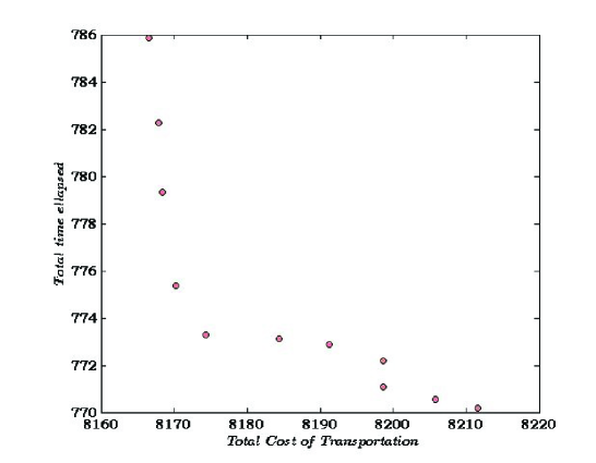
Figure 1: Approximated front for the proposed STP.

We have also optimize our proposed bi-objective STP by considering several randomly generated weight vectors to obtain multiple non-dominated solutions. Among these solutions we consider the best non-dominated solutions which are depicted in Fig. 1. These solutions are to be consider as members of the approximate front of our proposed bi-objective STP.

7 Conclusion

For transportation systems where full vehicles (e.g., light commercial vehicles, medium duty and heavy duty trucks, rail coaches, etc.) are to be considered for transportation of products, different types of issues appear in formulation of the problem. Like transportation cost of a vehicle which is irrespective of the fact whether the capacity of the vehicle is filed up or not; volume and weight capacities of the vehicles; limitation of number of certain types of vehicles, etc. Also, besides the travel time of a vehicle, loading and unloading times of products are also important which depend upon both the vehicle types and product characteristics. In his paper, we present a multi-objective multi-item solid transportation model by addressing all those issues. The presented problem is formulated with transportation time and cost parameters as fuzzy variables. We have formulated a chance-constrained programming model to solve the problem with fuzzy parameters, and then it is transformed into deterministic form. The deterministic multi-objective problem is solved with two multi-objective optimization techniques, namely, the fuzzy programming technique and global criterion method.

In the presented problem, the transportation time and cost parameters are considered as usual (type-1) fuzzy variables, however, this work can be extended with those parameters as represented by generalized type-2 or interval type-2 fuzzy variables.

References

- [1] E.E. Ammar and E.A. Youness, Study on multiobjective transportation problem with fuzzy numbers, Applied Mathematics and Computation 166 (2005), 241-253.
- [2] C.R. Bector and S. Chandra, Fuzzy mathematical programming and fuzzy matrix games, Springer, Berlin, Heidelberg, 2005.
- [3] A.K. Bit, M.P. Biswal and S.S. Alam, Fuzzy programming approach to multi-objective solid transportation problem, Fuzzy Sets and Systems 57 (1993), 183-194.
- [4] J.J. Buckley and E. Eslami, An Introduction to Fuzzy Logic and Fuzzy Sets, Physica-Verlag Heidelberg, New York, 2002.
- [5] S. Chanas and D. Kuchta, A concept of the optimal solution of the transportation problem with fuzzy cost coefficients, Fuzzy Sets and Systems 82 (1996), 299-305.
- [6] M. Chen and S.A. Ludwig, Color image segmentation using fuzzy C-regression model, Advances in Fuzzy Systems 2017 (2017), 1-15.
- [7] H. Dalman, N. Guzel and M. Sivri, A fuzzy set-based approach to multi-objective multi-item solid transportation problem under uncertainty, International Journal of Fuzzy Systems 18(4) (2016), 716-729.
- [8] A. Das, U. Bera and M. Maiti, Defuzzification of trapezoidal type-2 fuzzy variables and its application to solid transportation problem, Journal of Intelligent & Fuzzy Systems 30 (2016), 2431-2445.
- [9] D. Dubois and H. Prade, Possibility Theory: An Approach to Computerized Processing of Uncertainty, Plenum, New York, 1998.
- [10] M. Fei, P. Yi, Z. Kedong and Z. Jianyong, On-line hybrid fault diagnosis method for high voltage circuit breaker, Journal of Intelligent & Fuzzy Systems 33(5) (2017), 2763-2774.
- [11] M.R. Fegad, V.A. Jadhav and A.A. Muley, Finding an optimal solution of transportation problem using interval and triangular membership functions, European Journal of Scientific Research 60(3) (2011), 415-421.
- [12] P.K. Giri, M.K. Maiti and M. Maiti, Fully fuzzy fixed charge multi-item solid transportation problem, Applied Soft Computing 27 (2015), 77-91.
- [13] M. Hassaballah and A.Ghareeb, A framework for objective image quality measures based on intuitionistic fuzzy sets, Applied Soft Computing 57 (2017), 48-59.
- [14] K.B. Haley, The sold transportation problem, Operations Research 10 (1962), 448-463.
- [15] G. Jeon, M. Anisetti, E. Damiani and O. Monga, Real-time image processing systems using fuzzy and rough sets techniques, Soft Computing 22(5) 2018, 1381-1384.
- [16] F. Jiménez and J.L. Verdegay, Solving fuzzy solid transportation problems by an evolutionary algorithm based parametric approach, European Journal of Operational Research 117 (1999), 485-510.
- [17] P. Kundu, S. Kar and M. Maiti, Multi-objective solid transportation problems with budget constraint in uncertain environment, International Journal of Systems Science 45(8) (2014), 1668-1682.
- [18] P. Kundu, S. Kar and M. Maiti, Multi-item solid transportation problem with type-2 fuzzy parameters, Applied Soft Computing 31 (2015), 61-80.
- [19] P. Kundu, S. Majumder, S. Kar and M. Maiti, A method to solve linear programming problem with interval type-2 fuzzy parameters, Fuzzy Optimization and Decision Making (2018). DOI :10.1007/s10700-018-9287-2.
- [20] S.M. Lee and L.J. Moor, Optimizing transportation problems with multiple objectives, AIEE Transactions 5 (1973), 333-338.
- [21] C. Li, Z. Ding, D. Qian, and Y. Lv, Data-driven design of the extended fuzzy neural network having linguistic outputs, Journal of Intelligent & Fuzzy Systems, 34(1) (2018), 349-360.
- [22] Y. Li, K. Ida and M. Gen, Improved genetic algorithm for solving multi-objective solid transportation problem with fuzzy numbers, Computer and Industrial Engineering 33(3-4) (1997), 589-592.
- [23] L. Li and K.K. Lai, A fuzzy approach to the multi-objective transportation problem, Computers and Operation Research 27 (2000), 43-57.
- [24] B. Liu, Minimax chance constrained programming model for fuzzy decision systems, Information Sciences 112(1-4) (1998), 25-38.
- [25] B. Liu, A survey of credibility theory, Fuzzy Optimization and Decision Making 5(4) (2006), 387-408.
- [26] B. Liu and K. Iwamura, Chance constrained programming with fuzzy parameters, Fuzzy Sets and Systems 94(2) (1998), 227-237.
- [27] B. Liu and Y.K. Liu, Expected value of fuzzy variable and fuzzy expected value models, IEEE Transactions On Fuzzy Systems 10 (2002), 445-450.
- [28] P. Liu, Multiple attribute group decision making method based on interval-valued intuitionistic fuzzy power Heronian aggregation operators, Computers & Industrial Engineering 108 (2017), 199-212.
- [29] P. Liu and S.M. Chen, Multiattribute group decision making based on intuitionistic 2-tuple linguistic information, Information Sciences 430-431 (2018), 599-619.
- [30] P. Liu and S.M. Chen, Group decision making based on Heronian aggregation operators of intuitionistic fuzzy numbers, IEEE Transactions on Cybernetics 47(9)(2017), 2514-2530.
- [31] P. Liu, J. Liu and J.M. Merig , Partitioned Heronian means based on linguistic intuitionistic fuzzy numbers for dealing with multi-attribute group decision making, Applied Soft Computing 62 (2018), 395-422
- [32] P. Liu, S.M. Chen and J. Liu, Some intuitionistic fuzzy interaction partitioned Bonferroni mean operators and their application to multi-attribute group decision making, Information Sciences 411 (2017), 98-121.
- [33] J.M. Mendel, Uncertain rule-based fuzzy logic systems: Introduction and new directions, Prentice-Hall, NJ, 2001.
- [34] S. Nahmias, Fuzzy variable, Fuzzy Sets and Systems 1 (1978), 97-101.
- [35] P. Wang, Fuzzy contactability and fuzzy variables, Fuzzy Sets and Systems 8 (1982), 81-92.
- [36] A. Nagarjan and K. Jeyaraman, Solution of chance constrained programming problem for multi-objective interval solid transportation problem under stochastic environment using fuzzy approach, International Journal of Computer Applications 10(9) (2010), 19-29.
- [37] A. Ojha, B. Das, S. Mondal and M. Maity, An entropy based solid transportation problem for general fuzzy costs and time with fuzzy equality, Mathematical and Computer Modeling 50(1-2) (2009), 166-178.
- [38] B. Sinha, A. Das and U.K. Bera, Profit maximization solid transportation problem with trapezoidal interval type-2 fuzzy numbers, International Journal of Applied and Computational Mathematics 2(1) (2016), 41-56.
- [39] L. Yang and Y. Feng, A bicriteria solid transportation problem with fixed charge under stochastic environment, Applied Mathematical Modelling 31 (2007), 2668-2683.
- [40] L. Yang and L. Liu, Fuzzy fixed charge solid transportation problem and algorithm, Applied Soft Computing 7 (2007), 879-889.
- [41] F. Waiel and Abd El-wahed, A multi-objective transportation problem under fuzziness, Fuzzy Sets and Systems 117 (2001), 27-33.
- [42] W. Wang, Finite-time synchronization for a class of fuzzy cellular neural networks with time-varying coefficients and proportional delays, Fuzzy Sets and Systems 338 (2018), 40-49.
- [43] Y. Wu and J. Dong, Fault detection for T S fuzzy systems with partly unmeasurable premise variables, Fuzzy Sets and Systems 338 (2018), 136-156.
- [44] L.A. Zadeh, Fuzzy sets, Information and Control 8(3) (1965), 338-353.
- [45] L.A. Zadeh, Fuzzy sets as a basis for a theory of possibility, Fuzzy Sets and Systems 1 (1978), 3-28.
- [46] H.-J. Zimmermann, Fuzzy programming and linear programming with several objective functions, Fuzzy Sets and Systems 1 (1978), 45-55.