A multi-objective reliability-redundancy allocation problem with active redundancy and interval type-2 fuzzy parameters

Abstract

This paper considers a multi-objective reliability-redundancy allocation problem (MORRAP) of a series-parallel system, where system reliability and system cost are to be optimized simultaneously subject to limits on weight, volume, and redundancy level. Precise computation of component reliability is very difficult as the estimation of a single number for the probabilities and performance levels are not always possible, because it is affected by many factors such as inaccuracy and insufficiency of data, manufacturing process, environment in which the system is running, evaluation done by multiple experts, etc. To cope with impreciseness, we model component reliabilities as interval type-2 fuzzy numbers (IT2 FNs), which is more suitable to represent uncertainties than usual or type-1 fuzzy numbers. To solve the problem with interval type-2 fuzzy parameters, we first apply various type-reduction and defuzzification techniques, and obtain corresponding defuzzified values. As maximization of system reliability and minimization of system cost are conflicting to each other, so to obtain compromise solution of the MORRAP with defuzzified parameters, we apply five different multi-objective optimization methods, and then corresponding solutions are analyzed. The problem is illustrated numerically for a real-world MORRAP on pharmaceutical plant, and solutions are obtained by standard optimization solver LINGO, which is based on gradient-based optimization - Generalized Reduced Gradient (GRG) technique.

Keywords: Multi-objective optimization; Reliability; Redundancy allocation; Interval type-2 fuzzy set.

1 Introduction

An industrial or a mechanical system such as aircraft, nuclear plants, lighting system, material handling systems, pharmaceutical plant, civil engineering systems, and so on is composed of numerous complex components. The reliability, i.e., the probability that a system performs satisfactorily over a certain period of time depends on each of its constituent components and the system design. The study of reliability optimization relates to enhance the reliability of a system so that the system can be operational satisfactorily for the maximum possible time. Reliability of a system can be improved by using high reliable components and adding redundant (standby) components. However, this may increase the system cost. Further designing of system structure also depends on various resource/engineering constraints related to cost, volume, weight, and energy consumption, etc. Reliability-redundancy allocation problem (RRAP) (Kuo and Prasad, 2000) is the problem of maximizing system reliability through redundancy (Caserta and Voß, 2015) and component reliability choices subject to the applicable resource constraints. However, in addition to maximization of system reliability, if the system cost or weight has to be minimized simultaneously, then the problem becomes the multi-objective reliability-redundancy allocation problem (MORRAP) (Ardakan and Rezvan, 2018; Cao et al., 2013; Garg and Sharma, 2013; Huang et al., 2009; Khalili-Damghani et al., 2013; Muhuri et al., 2018; Rao and Dhingra, 1992; Safari, 2012). The main goal of such MORRAP is to determine the optimal component reliabilities and number of redundant components in each of the subsystems to maximize the system reliability and minimize the system cost simultaneously subject to several resource constraints.

Practically, exact computation of reliability is challenging and is associated with uncertainties due to various reasons. Notably, the estimation of a single number for the probabilities and performance levels is very difficult (Cheng and Mon, 2008). Some reasons come from inaccuracy and insufficiency of data, data collection from multiple sources or evaluation done by multiple experts, etc. Some other key sources of uncertainties are uncertainty factors in manufacturing process (like quality assurance controls, work management and execution, maintenance activities) and environmental factors (the reliability of components depends on the factors like temperature, voltage, humidity of the environment in which the associated system is running). So, it is not always possible to precisely determine the reliability of a component. Many researchers have investigated RRAP with various uncertain parameters such as interval-valued (Sahoo et al., 2012; Garg et al., 2014; Roy et al., 2014; Xu and Liao, 2016; Zhang and Chen, 2016), and fuzzy parameters (Mahapatra and Roy, 2006; Yao et al., 2008; Cheng and Mon, 2008; Garg et al., 2013; Kumar and Yadav, 2012; Sriramdas et al., 2014; Muhuri et al., 2018). Most of the RRAP with fuzzy parameters considered type-1 fuzzy numbers (T1 FNs) for modeling the uncertainties (Chen, 1994; Aliev and Kara, 2004; Yao et al., 2008; Jamkhaneh and Nozari, 2012).

Type-2 fuzzy sets (T2 FSs) (for details see Mendel and John, 2002) are proved to be more suitable in many instances to represent uncertainties than ordinary or type-1 fuzzy sets. A Type-2 fuzzy set is a generalization of type-1 fuzzy set, and has an extra degree of freedom to represent uncertainties because of its secondary membership function. Interval type-2 fuzzy set (IT2 FS) (Mendel et al., 2006), a special case of general T2 FS has been successfully used to model uncertain parameters in many instances like data collected from multiple sources, opinion taken from several experts, information given by approximate intervals or linguistic terms, etc. Specifically, it is showed by many researchers that to deal with linguistic uncertainties (Mendel, 2003, 2007a, 2007b; Liu and Mendel, 2008; Miller et al., 2012), approximate intervals (like two endpoints of the intervals are not certain) (Liu and Mendel, 2008) or several membership functions (Pagola et al., 2013), interval type-2 fuzzy set is an appropriate tool. Not only that, Mendel (2003, 2007a, 2007b) explained and showed that modeling linguistic information using type-1 fuzzy set is not scientific, instead one should use type-2 fuzzy set, specifically interval type-2 fuzzy set. As we mention earlier, there are several research work has been done on RRAP with T1 FNs. However, there are very few research works on RRAP with type-2 fuzzy numbers available in the literature (Muhuri et al., 2018). The significant contributions of the present investigation are as follows:

• We formulate a MORRAP of a series-parallel system with the approximate reliability of each component of a subsystem represented as interval type-2 fuzzy numbers (IT2 FNs). Most of the previous research work has been investigated RRAP with interval numbers or T1 FNs.

• We not only explain but also illustrate numerically that modeling uncertain parameters (reliabilities) using IT2 FNs leads to the better performance than that of using T1 FNs, i.e. our investigation suggest that we can model system with higher system reliability and less system cost.

• We apply various type-reduction and defuzzification techniques to obtain corresponding defuzzified values of IT2 FNs, and comparative study has been presented.

• To deal with conflicting objectives we apply five different multi-objective optimization techniques to obtain solution of the problem. As a result a decision maker can choose appropriate result according to his/her preference or as situation demand.

In our considered MORRAP there are two conflicting objectives, namely, maximization of system reliability and minimization of system cost. Construction of IT2 FNs to represent imprecise component reliabilities has been done by using a modified algorithm which was initially proposed by Muhuri et al. (2018). To solve MORRAP with interval type-2 fuzzy parameters, we first apply various type-reduction and defuzzification techniques to obtain corresponding defuzzified values. To deal with two conflicting objectives we then apply five different multi-objective optimization methods, and obtain compromise solution of the problem. The problem is also solved by modeling component reliabilities as T1 FNs, and the obtained result is compared with the result for the same problem with IT2 FNs. The rest of the paper is organized as follows. Section 2 provides brief introduction of type-2 fuzzy set. The detail of the problem (MORRAP) formulation is presented in Section 3. Section 4 discusses some type-reduction and defuzzification techniques in brief. Section 5 presents some multi-objective optimization techniques in detail. In Section 6, the problem and methods are illustrated numerically for a real-world MORRAP on pharmaceutical plant. Finally, Section 7 concludes the paper.

2 Preliminaries

2.1 Type-2 fuzzy set

Type-2 fuzzy set (T2 FS) is an extension of usual or type-1 fuzzy set (T1 FS). It is a fuzzy set with fuzzy membership function, i.e., membership grade of each element in the set is no longer a precise (crisp) value but a fuzzy set.

Definition 1

A type-2 fuzzy set $\tilde{\tilde{A}}$ (Mendel and John, 2002) in a space of points (objects) $X$ is characterized by a type-2 membership function $\mu_{\tilde{\tilde{A}}}:X\times J_{x}\rightarrow[0,1]$, and is defined as

$$\tilde{\tilde{A}}=\{((x,u),\mu_{\tilde{\tilde{A}}}(x,u)):~{}\forall x\in X,~{}\forall u\in J_{x}\subseteq[0,1]\},$$

where $J_{x}\subseteq[0,1]$ is the primary membership of $x\in X$, and $0\leq\mu_{\tilde{\tilde{A}}}(x,u)\leq 1$ for all $x\in X$, $u\in J_{x}$. $\tilde{\tilde{A}}$ is also expressed as

$$\tilde{\tilde{A}}=\int_{x\in X}\int_{u\in J_{x}}\mu_{\tilde{\tilde{A}}}(x,u)/(x,u)~{},~{}J_{x}\subseteq[0,1],$$

where $\int\int$ denotes union over all admissible $x$ and $u$. For discrete universes of discourse, $\int$ is replaced by $\sum$.
For particular $x=x^{\prime}\in X$, $\mu_{\tilde{\tilde{A}}}(x^{\prime},u)$ $\forall u\in J_{x^{\prime}}$, is called secondary membership of $x^{\prime}$. The amplitude of a secondary membership function is called a secondary membership grade. Thus $\mu_{\tilde{\tilde{A}}}(x^{\prime},u^{\prime})$, $u^{\prime}\in J_{x^{\prime}}$ is secondary membership grade of $(x^{\prime},u^{\prime})$ which represents the grade of membership that the point $x^{\prime}$ has the primary membership $u^{\prime}$.

Definition 2

An interval type-2 fuzzy set (IT2 FS) (Mendel et al., 2006) is a special case of T2 FS where all the secondary membership grades are 1, i.e., $\mu_{\tilde{\tilde{A}}}(x,u)=1$ for all $(x,u)\in X\times J_{x}$. An IT2 FS $\tilde{\tilde{A}}$ can be written as

$$\tilde{\tilde{A}}=\int_{x\in X}\int_{u\in J_{x}}1/(x,u)=\int_{x\in X}\left.\left[\int_{u\in J_{x}}1/u\right]\middle/x\right.,~{}J_{x}\subseteq[0,1].$$

As the secondary membership grades are 1, an IT2 FS can be characterized by the footprint of uncertainty (FOU) which is the union of all primary memberships $J_{x}$ in a bounded region, so that it is defined as

$$FOU(\tilde{\tilde{A}})=\bigcup_{x\in X}~{}J_{x}.$$

The FOU (see Fig. 1) is bounded by an upper membership function (UMF) $\bar{\mu}_{\tilde{\tilde{A}}}(\cdot)$ and a lower membership function (LMF) $\underline{\mu}_{\tilde{\tilde{A}}}(\cdot)$, both of which are the membership functions of T1 FSs, and $J_{x}=[\underline{\mu}_{\tilde{\tilde{A}}}(x),\bar{\mu}_{\tilde{\tilde{A}}}(x)]$, $\forall~{}x\in X$. In this view, the IT2 FS can be represented by $(\tilde{A^{U}},\tilde{A^{L}})$, where $\tilde{A^{U}}$ and $\tilde{A^{L}}$ are T1 FSs. The support of IT2 FS $\tilde{\tilde{A}}$ can written as $supp(\tilde{\tilde{A}})=\{x\in X:\bar{\mu}_{\tilde{\tilde{A}}}(x)>0\}$.

Definition 3

Interval type-2 fuzzy number (IT2 FN): An interval type-2 fuzzy number (IT2 FN) (Hesamian, 2017) is an IT2 FS on set of real numbers $\mathbb{R}$, whose upper and lower membership functions are membership functions of T1 FNs.

For example, Fig. 1 represents a triangular IT2 FN $\tilde{\tilde{A}}=(\tilde{A^{U}},\tilde{A^{L}})=((2,4,6),(3,4,5))$, where $\tilde{A^{U}}$ and $\tilde{A^{L}}$ are triangular fuzzy numbers having following membership functions:

$$\mu_{\tilde{A^{U}}}(x)=\bar{\mu}_{\tilde{\tilde{A}}}(x)=\left\{\begin{array}[]{ll}\frac{x-2}{2},&\hbox{if $2\leq x\leq 4$;}\\ 1,&\hbox{if $x=4$;}\\ \frac{6-x}{2},&\hbox{if $4\leq x\leq 6$;}\\ 0,&\hbox{otherwise.}\end{array}\right.~{}\mu_{\tilde{A^{L}}}(x)=\underline{\mu}_{\tilde{\tilde{A}}}(x)=\left\{\begin{array}[]{ll}x-3,&\hbox{if $3\leq x\leq 4$;}\\ 1,&\hbox{if $x=4$;}\\ 5-x,&\hbox{if $4\leq x\leq 5$;}\\ 0,&\hbox{otherwise.}\end{array}\right.$$

The arithmetic operations between two triangular IT2 FNs $\tilde{\tilde{A_{1}}}=(\tilde{A_{1}^{U}},\tilde{A_{1}^{L}})=((a_{11}^{U},a_{12}^{U},a_{13}^{U}),(a_{11}^{L},a_{12}^{L},a_{13}^{L}))$ and $\tilde{\tilde{A_{2}}}=(\tilde{A_{2}^{U}},\tilde{A_{2}^{L}})=((a_{21}^{U},a_{22}^{U},a_{23}^{U}),(a_{21}^{L},a_{22}^{L},a_{23}^{L}))$ are defined as follows:
Addition operation: $\tilde{A_{1}}\oplus\tilde{A_{2}}=(\tilde{A_{1}^{U}},\tilde{A_{1}^{L}})\oplus(\tilde{A_{2}^{U}},\tilde{A_{2}^{L}})$
$=((a_{11}^{U}+a_{21}^{U},a_{12}^{U}+a_{22}^{U},a_{13}^{U}+a_{23}^{U}),(a_{11}^{L}+a_{21}^{L},a_{12}^{L}+a_{22}^{L},a_{13}^{L}+a_{23}^{L})),$
Multiplication operation: $\tilde{A_{1}}\otimes\tilde{A_{2}}=(\tilde{A_{1}^{U}},\tilde{A_{1}^{L}})\otimes(\tilde{A_{2}^{U}},\tilde{A_{2}^{L}})$
$=((a_{11}^{U}\times a_{21}^{U},a_{12}^{U}\times a_{22}^{U},a_{13}^{U}\times a_{23}^{U}),(a_{11}^{L}\times a_{21}^{L},a_{12}^{L}\times a_{22}^{L},a_{13}^{L}\times a_{23}^{L})).$
The arithmetic operations between triangular IT2 FN $\tilde{\tilde{A_{1}}}$ and a real number $r$ are defined as follows:
$r\tilde{\tilde{A_{1}}}=((r\times a_{11}^{U},r\times a_{12}^{U},r\times a_{13}^{U}),(r\times a_{11}^{L},r\times a_{12}^{L},r\times a_{13}^{L})),$
$\frac{\tilde{\tilde{A_{1}}}}{r}=((\frac{1}{r}\times a_{11}^{U},\frac{1}{r}\times a_{12}^{U},\frac{1}{r}\times a_{13}^{U}),(\frac{1}{r}\times a_{11}^{L},\frac{1}{r}\times a_{12}^{L},\frac{1}{r}\times a_{13}^{L}))$, where $r>0$.

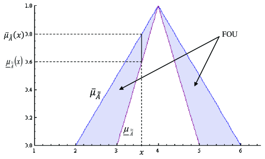
Figure 1: Triangular IT2 FN $\tilde{\tilde{A}}=((2,4,6),(3,4,5))$.

3 A Multi-objective reliability-redundancy allocation problem (MORRAP)

Generally, complex systems are composed of several subsystems (stages), each having more than one component. In reliability context, system designing mainly concern with improvement of overall system reliability, which may be subject to various resource/engineering constraints associated with system cost, weight, volume, and energy consumption. This may be done (i) by incorporating more reliable components (units) and/or (ii) incorporating more redundant components. In case of the second approach, optimal redundancy is mainly taken into consideration for the economical design of systems. Again the reliability optimization concerned with redundancy allocation is generally classified into two categories: (i) maximization of system reliability subject to various resource constraints; and (ii) minimization of system cost subject to the condition that the associated system reliability is required to satisfy a desired level. However, if maximization of system reliability and minimization of the system cost have to be done simultaneously, then the problem becomes the multi-objective reliability-redundancy allocation problem (MORRAP). So, the main goal of MORRAP is to determine the optimal component reliabilities and number of redundant components in each of the subsystems to maximize the system reliability and minimize the system cost simultaneously subject to several resource constraints.

Here, we have considered a MORRAP for a series-parallel system configuration (Huang et al., 2009; Garg and Sharma, 2013). A series-parallel system usually has $m$ (say) independent subsystems arranged in series, and in each subsystem, there are $n_{i}$ (say) $(i=1,2,...,m)$ components, which are arranged in parallel. A reliability block diagram (RBD) of this series-parallel system is depicted in Fig. 2, where small rectangular blocks represent the components in each of the $m$ subsystems. The reliability block diagram provides a graphical representation of the system that can be used to analyze the relationship between component states and the success or failure of a specified system. As seen from Fig. 2, in each subsystem the components are arranged in parallel, so each of the subsystems can work if at least one of its components works. Again as these subsystems are arranged in series, the whole system can work if all the subsystems work. Obviously, reliability of the series-parallel system is the product of all the associated subsystem reliabilities. For the considered MORRAP, the objective functions are maximization of system reliability and minimization of system cost, subject to limits on weight, volume, and redundancy level. Also, the problem considers the active redundancy strategy (i.e., all the components in each subsystem are active and arranged in parallel).

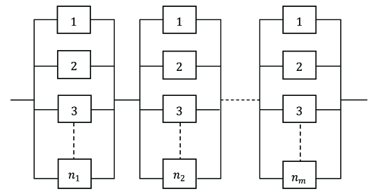
Figure 2: Reliability block diagram of series-parallel system.

For the mathematical formulation of the problem we use the following notations:

$m$	Number of subsystems
$n_{i}$	Number of components in subsystem $i$ ($i=1,2,...,m)$
$r_{i}$	Reliability of each of the components in $i$th subsystem
$R_{s}$	System reliability
$C_{s}$	System cost
$c(r_{i})$	Cost of the each component with reliability $r_{i}$ at subsystem $i$
$\alpha_{i}$	Constants representing the physical characteristic (scaling factor) of the cost-reliability
	curve of each component with reliability $r_{i}$ at subsystem $i$
$\beta_{i}$	Constants representing the physical characteristic (shaping factor) of the cost-reliability
	curve of each component with reliability $r_{i}$ at subsystem $i$
$T$	Operating time during which the component must not fail
$w_{i}$	Weight of each component of the subsystem $i$
$W_{s}$	System weight
$W$	Upper limit on the weight of the system
$v_{i}$	Volume of each component of the subsystem $i$
$V_{s}$	System volume
$V$	Upper limit on the volume of the system

It is assumed that all the components for individual subsystem are identical, all redundancies are active, failures of individual components are independent, and each component can only be in one of two states, i.e., either working or failed. Now the mathematical formulation of the MORRAP is as follows:

$$\text{Max}~{}R_{s} = \prod_{i=1}^{m}~{}\left[1-(1-r_{i})^{n_{i}}\right],$$ (1)

$$Min~{}C_{s} = \sum_{i=1}^{m}c(r_{i})(n_{i}+\exp(n_{i}/4)),$$ (2)

subject to $$V_{s}=\sum_{i=1}^{m}v_{i}n_{i}^{2}~{}\leq V,$$ (4)

$$W_{s}=\sum_{i=1}^{m}w_{i}(n_{i}\cdot\exp(n_{i}/4))\leq W,$$

$$r_{i,min}\leq r_{i}\leq r_{i,max},1\leq n_{i}\leq n_{i,max},r_{i}\in(0,1),i=1,2,...,m.$$ (5)

For the presented model, cost of the each component is an increasing function of the component reliability or conversely a decreasing function of the failure rate (hazard rate) of the component, where failure times of components follow exponential distribution. So the reliability of each of the component in subsystem $i$,

$$r_{i}=e^{-\lambda_{i}T},~{}\lambda_{i}>0,$$ (6)

and consequently the hazard rate is $\lambda_{i}$, where $T$ be the operating time during which the component will not fail. As cost of the each component in the $i$-th subsystem, $c(r_{i})$, is a decreasing function of the hazard rate, it is represented as

$$c(r_{i})=\alpha_{i}\lambda_{i}^{-\beta_{i}},$$ (7)

where $\alpha_{i}$ and $\beta_{i}$ are constants. Equations (6) and (7) together gives $c(r_{i})=\alpha_{i}\left(\frac{-T}{ln(r_{i})}\right)^{\beta_{i}}$. Now, each subsystem is comprised of some components connected in parallel. The factor $\exp(n_{i}/4)$ is incorporated due to the interconnecting hardware between the parallel components (Rao and Dhingra, 1992; Prasad and Kuo, 2000; Wang et al., 2009; Ardakan and Rezvan, 2018). Total volume of the system $(V_{s})$ which consists of the volume of the each component as well as space between the components and space between the subsystems, is represented in equation (4). Here $n_{i,max}$ represents the maximum number of components allowed in subsystem $i$ arranged in parallel, and $r_{i,min}$ and $r_{i,max}$ respectively the minimum and maximum reliability limits of each component in subsystem $i$.

3.1 MORRAP with interval type-2 fuzzy parameters

As discussed in the introduction, the component reliability in a system cannot be always precisely measured as crisp values, but may be determined as approximate values like “about 0.6” or approximate intervals with imprecise end points. Some of the reasons are inaccuracy and insufficiency of data, manufacturing uncertainty, environmental issues (like temperature, humidity of the environment in which the system is running), evaluation done by multiple experts or data collected from multiple sources, etc. So to cope with the ambiguity/approximation we associate a degree of membership to each value of reliability. Here the approximate reliability of each component of a subsystem is represented by IT2 fuzzy number and is denoted by $\tilde{\tilde{r}}_{i}$, $i=1,2,...,m$. The assumption of IT2 FN to represent uncertainty is vary reasonable when value of a parameter is given by approximate interval (like the two end-points of the interval are not exact), linguistic terms, etc. Now the above MORRAP (1)-(5) becomes

$$\text{Max}~{}\tilde{\tilde{R}}_{s}=\prod_{i=1}^{m}~{}\left[1-(1-\tilde{\tilde{r}}_{i})^{n_{i}}\right],$$ (8)

$$Min~{}\tilde{\tilde{C}}_{s}=\sum_{i=1}^{m}\alpha_{i}\left(\frac{-T}{ln(\tilde{\tilde{r}}_{i})}\right)^{\beta_{i}}(n_{i}+\exp(n_{i}/4))$$ (9)

$$\text{subject to }~{}(\ref{eqmorp3})-(\ref{eqmorp5}).$$ (10)

To solve this problem we use different type-reduction and corresponding defuzzification strategies to convert the problem with IT2 fuzzy parameters to the problem with defuzzified parameters. Then we use various multi-objective techniques to solve the deterministic bi-objective problem. To construct interval type-2 fuzzy membership function for the reliability $\tilde{\tilde{r}}_{i}$ having support $supp(\tilde{\tilde{r}}_{i})\subseteq[a,b]\subset[0,1]$ we use the following algorithm. To construct this algorithm we modified the Algorithm-1 of Muhuri et al. (2018) to ensure that the support of $\tilde{\tilde{r}}_{i}$ must lie within $(0,1)$.

Algorithm: Generation of T1 FN $(\tilde{r}_{i})$ and IT2 FN $(\tilde{\tilde{r}}_{i})$

Step 1:

Take $r_{i}\in[a,b]$.

Step 2:

Find the values of $r_{i}^{l}$ and $r_{i}^{u}$ as follows:
$r_{i}^{l}=a+(r_{i}-a)*rand$
$r_{i}^{u}=b-(b-r_{i})*rand$

Step 3:

Construct the T1 FN $\tilde{r}_{i}=(r_{i}^{l},r_{i},r_{i}^{u})$. // This step should be skipped for generation of IT2 FN.

Step 4:

Find the values of $r_{i1}^{l}$ and $r_{i3}^{l}$ as follows:
$r_{i1}^{l}=r_{i}^{l}+(r_{i}-r_{i}^{l})*rand$
$r_{i3}^{l}=r_{i}^{u}-(r_{i}^{u}-r_{i})*rand$

Step 5:

Find the values of $r_{i1}^{u}$ and $r_{i3}^{u}$ as follows:
$r_{i1}^{u}=r_{i}^{l}-(r_{i}^{l}-a)*rand$
$r_{i3}^{u}=r_{i}^{u}+(b-r_{i}^{u})*rand$

Step 6:

Construct the IT2 FN $\tilde{\tilde{r}}_{i}=((r_{i1}^{u},r_{i},r_{i3}^{u}),(r_{i1}^{l},r_{i},r_{i3}^{l}))$.

In the next section we have briefly introduced different type-reduction and defuzzification strategies of interval type-2 fuzzy set.

4 Type-reduction and defuzzification strategies

Here, we discuss some type-reduction and defuzzification strategies those are investigated in this study to obtain corresponding type-reduced set and defuzzified values of interval type-2 fuzzy parameters. These methods are given in detail in the corresponding references. However, we present the methods briefly to provide a ready reference to readers.

4.1 Karnik-Mendel (KM) algorithm

Karnik and Mendel (2001) introduced the concept of centroid of T2 FS by which it can be reduced to a T1 FS (Liu, 2008). The computational procedure to find centroid of an IT2 FS $\tilde{\tilde{A}}$ starts with discretization (if the domain is not discrete) of the continuous domain into finite number of points $x_{i}$, $i=1,2,...,N$ which are sorted in an ascending order. Then the centroid of the IT2 FS is given by $[y_{l},y_{r}]$ and corresponding defuzzified value is $C(\tilde{\tilde{A}})=(y_{l}+y_{r})/2$, where

$$y_{l}=\frac{\sum_{i=1}^{L}x_{i}\bar{\mu}_{\tilde{\tilde{A}}}(x_{i})+\sum_{i=L+1}^{N}x_{i}\underline{\mu}_{\tilde{\tilde{A}}}(x_{i})}{\sum_{i=1}^{L}\bar{\mu}_{\tilde{\tilde{A}}}(x_{i})+\sum_{i=L+1}^{N}\underline{\mu}_{\tilde{\tilde{A}}}(x_{i})},$$

$$y_{r}=\frac{\sum_{i=1}^{R}x_{i}\underline{\mu}_{\tilde{\tilde{A}}}(x_{i})+\sum_{i=R+1}^{N}x_{i}\bar{\mu}_{\tilde{\tilde{A}}}(x_{i})}{\sum_{i=1}^{R}\underline{\mu}_{\tilde{\tilde{A}}}(x_{i})+\sum_{i=R+1}^{N}\bar{\mu}_{\tilde{\tilde{A}}}(x_{i})}.$$

Here $L$ and $R$ are switch points which are calculated by KM algorithm (Karnik and Mendel, 2001; Mendel and Liu, 2007). It is obvious that for large $N$, i.e. for $(x_{i+1}-x_{i})\rightarrow 0$, the discretization of continuous domain is legitimate for computation of centroid. Also, it is observed that (Mendel and Liu, 2007) for IT2 FS with symmetrical membership function, choice of $N$ has less effect on computed centroid.

4.2 Uncertainty bound (UB)

Wu and Mendel (2002) provided inner- and outer-bound sets for type-reduced set, which can not only be used to compute left and right end points of the type-reduced set, but can also be used to derive the defuzzified output of an IT2 FS. As compared to KM algorithm, this method can performed without type-reduction and $x_{i}$s need not be sorted, so that it removes computational burden of type-reduction. The approximation of the type-reduced set by its inner- and outer-bound sets is given by $[y_{l},y_{r}]$, where $y_{l}=(\underline{y}_{l}+\bar{y}_{l})/2$ and $y_{r}=(\underline{y}_{r}+\bar{y}_{r})/2$, and corresponding defuzzified output is $(y_{l}+y_{r})/2$,

$$\bar{y}_{l}=\min\{y^{(0)},y^{(N)}\}$$

$$\underline{y}_{r}=\max\{y^{(0)},y^{(N)}\}$$

$$\underline{y}_{l}=\bar{y}_{l}-\left[\frac{\sum_{i=1}^{N}\left(\bar{\mu}_{\tilde{\tilde{A}}}(x_{i})-\underline{\mu}_{\tilde{\tilde{A}}}(x_{i})\right)}{\sum_{i=1}^{N}\bar{\mu}_{\tilde{\tilde{A}}}(x_{i})\sum_{i=1}^{N}\underline{\mu}_{\tilde{\tilde{A}}}(x_{i})}\times\frac{\sum_{i=1}^{N}\underline{\mu}_{\tilde{\tilde{A}}}(x_{i})(x_{i}-x_{1})\sum_{i=1}^{N}\bar{\mu}_{\tilde{\tilde{A}}}(x_{i})(x_{N}-x_{i})}{\sum_{i=1}^{N}\underline{\mu}_{\tilde{\tilde{A}}}(x_{i})(x_{i}-x_{1})+\sum_{i=1}^{N}\bar{\mu}_{\tilde{\tilde{A}}}(x_{i})(x_{N}-x_{i})}\right]$$

$$\bar{y}_{r}=\underline{y}_{r}+\left[\frac{\sum_{i=1}^{N}\left(\bar{\mu}_{\tilde{\tilde{A}}}(x_{i})-\underline{\mu}_{\tilde{\tilde{A}}}(x_{i})\right)}{\sum_{i=1}^{N}\bar{\mu}_{\tilde{\tilde{A}}}(x_{i})\sum_{i=1}^{N}\underline{\mu}_{\tilde{\tilde{A}}}(x_{i})}\times\frac{\sum_{i=1}^{N}\bar{\mu}_{\tilde{\tilde{A}}}(x_{i})(x_{i}-x_{1})\sum_{i=1}^{N}\underline{\mu}_{\tilde{\tilde{A}}}(x_{i})(x_{N}-x_{i})}{\sum_{i=1}^{N}\bar{\mu}_{\tilde{\tilde{A}}}(x_{i})(x_{i}-x_{1})+\sum_{i=1}^{N}\underline{\mu}_{\tilde{\tilde{A}}}(x_{i})(x_{N}-x_{i})}\right]$$

$$y^{(0)}=\frac{\sum_{i=1}^{N}x_{i}\underline{\mu}_{\tilde{\tilde{A}}}(x_{i})}{\sum_{i=1}^{N}\underline{\mu}_{\tilde{\tilde{A}}}(x_{i})}$$

$$y^{(N)}=\frac{\sum_{i=1}^{N}x_{i}\bar{\mu}_{\tilde{\tilde{A}}}(x_{i})}{\sum_{i=1}^{N}\bar{\mu}_{\tilde{\tilde{A}}}(x_{i})}.$$

4.3 Nie-Tan (N-T) method

Nie and Tan (2008) proposed a type-reduction method which is formulated using the vertical-slice representation of an IT2 FS. In this method, type reduction and defuzzification are performed together. As of the previous two methods, if the domain of IT2 FS is continuous then it is discreteized into finite number of points $x_{i}$, $i=1,2,...,N$. Then the centroid (or defuzzified value) of the IT2 FS $\tilde{\tilde{A}}$ can be expressed as

$$C(\tilde{\tilde{A}})=\frac{\sum_{i=1}^{N}x_{i}\bar{\mu}_{\tilde{\tilde{A}}}(x_{i})+\sum_{i=1}^{N}x_{i}\underline{\mu}_{\tilde{\tilde{A}}}(x_{i})}{\sum_{i=1}^{N}\bar{\mu}_{\tilde{\tilde{A}}}(x_{i})+\sum_{i=1}^{N}\underline{\mu}_{\tilde{\tilde{A}}}(x_{i})}.$$

The above formulation of the crisp output of an IT2 FS depends only on the lower and upper bounds of its FOU. The computational complexity of the N-T method is lower than the uncertainty bounds method and the KM algorithm.

4.4 Geometric centroid

Coupland and John (2007) introduced the idea of geometric centroid of an IT2 FS by converting the region bounded by upper and lower membership functions (which are piecewise linear) to a closed polygon. The polygon consists of ordered coordinate points of the upper bound of $\tilde{\tilde{A}}$ followed by the lower bound of $\tilde{\tilde{A}}$ in reverse order. Let the polygon is given by $((x_{1},y_{1}),(x_{2},y_{2}),...,(x_{M},y_{M}))$, where $y_{i}$ is either $\bar{\mu}_{\tilde{\tilde{A}}}(x_{i})$ or $\underline{\mu}_{\tilde{\tilde{A}}}(x_{i})$ according to the position of the coordinate point. Then the defuzzified output is taken as the centroid (center of the polygon) of the polygon which is given by

$$\frac{\sum_{i=1}^{M-1}(x_{i}+x_{i+1})(x_{i}y_{i+1}-x_{i+1}y_{i})}{3\sum_{i=1}^{M-1}(x_{i}y_{i+1}-x_{i+1}y_{i})}.$$

5 Multi-objective optimization techniques

The problem (8)-(10) is a bi-objective problem with one objective as maximization and another as minimization. To solve this problem with defuzzified parameters we apply different multi-objective optimization techniques, namely, global criterion method, weighted sum method, desirability function approach, fuzzy programming technique and NIMBUS which are discussed briefly in this section. Consider a general multi-objective optimization problem with some objectives to be maximized and some others to be minimized:

$$\text{Max}~{}\{f_{1}(x),f_{2}(x),...,f_{K}(x)\}$$ (11)

$$\text{Min}~{}\{g_{1}(x),g_{2}(x),...,g_{M}(x)\}$$ (12)

$$\text{s.t.}~{}x\in D,$$ (13)

where $D$ is the set of feasible solutions.
We use the following notations in describing the methods: $f_{i}^{\max}=\text{Max}~{}f_{i}(x)$, $f_{i}^{\min}=\text{Min}~{}f_{i}(x)$, $g_{j}^{\max}=\text{Max}~{}g_{j}(x)$, and $g_{j}^{\min}=\text{Min}~{}g_{j}(x)$, $i=1,2,...,K$ and $j=1,2,...,M$ subject to $x\in D$ in each case. We also denote the optimal solution of single objective problem (considering only one objective $f_{i}$ or $g_{j}$ ignoring all other objectives) as $x_{f_{i}}^{*}$ and $x_{g_{j}}^{*}$ respectively for $i=1,2,...,K$ and $j=1,2,...,M$. The ideal objective vector for the above problem is $(f_{1}^{\max},f_{2}^{\max},...,f_{K}^{\max},g_{1}^{\min},g_{2}^{\min},...,g_{M}^{\min})$.

5.1 Global criteria method

By the method of global criteria (Zeleny, 1973; Miettinen, 2012) a compromise solution is achieved by minimizing the sum of the differences between ideal objective value and the respective objective function values in the set of feasible solution. The ideal objective value may be taken as the minimum value of the objective function for minimization problem, and maximum value for maximization problem obtained as by solving the multi-objective problem as a single objective problem, considering each objective individually. The method may be described by the following steps for solving the multi-objective problem (11)-(13):
Step 1: Construct single objective problems by taking each objective function individually.
Step 2: For each single objective problem, determine the ideal objective vector $(f_{1}^{\max},f_{2}^{\max},...,f_{K}^{\max},g_{1}^{\min},g_{2}^{\min},...,g_{M}^{\min})$ and corresponding values of $(f_{1}^{\min},f_{2}^{\min},...,f_{K}^{\min},g_{1}^{\max},\\ g_{2}^{\max},...,g_{M}^{\max})$.
Step 3: Formulate the following auxiliary problem using normalized Minkowski distance ($L_{p}$ norm):

$$Min~{}G(x)$$

s.t. $x\in D,$

$$G(x)=\text{Min}\left\{\sum_{i=1}^{K}\left(\frac{f_{i}^{\max}-f_{i}(x)}{f_{i}^{\max}-f_{i}^{\min}}\right)^{p}+\sum_{j=1}^{M}\left(\frac{g_{j}(x)-g_{j}^{\min}}{g_{j}^{\max}-g_{j}^{\min}}\right)^{p}\right\}^{\frac{1}{p}},$$

$$or,~{}G(x)=\text{Min}\left\{\sum_{i=1}^{K}\left(\frac{f_{i}^{\max}-f_{i}(x)}{f_{i}^{\max}}\right)^{p}+\sum_{j=1}^{M}\left(\frac{g_{j}(x)-g_{j}^{\min}}{g_{j}^{\min}}\right)^{p}\right\}^{\frac{1}{p}},$$

where $1\leq p\leq\infty$. An usual value of $p$ is 2.

5.2 Weighted sum method

In weighted sum method, multiple objectives are aggregated to convert into a single objective by employing weight to each objective. The weighting coefficients denote the relative importance of the objectives. Now the values of different objectives may have different order of magnitude, so it is necessary to normalize the objectives, in order to make solution consistent with the weights as assigned to the objectives. The objective functions may be converted to their normal forms as follows:

$$f_{i}^{norm}=\frac{f_{i}(x)-f_{i}^{\min}}{f_{i}^{\max}-f_{i}^{\min}},~{}\text{(for objectives to be maximized)}$$

$$g_{j}^{norm}=\frac{g_{j}^{\max}-g_{j}(x)}{g_{j}^{\max}-g_{j}^{\min}},~{}\text{(for objectives to be minimized)}.$$

A weight $w_{i}$ is taken for every objective and then aggregated to form the following problem:

$$\text{Max}~{}\left(\sum_{i=1}^{K}w_{i}f_{i}^{norm}+\sum_{j=1}^{M}w_{K+j}~{}g_{j}^{norm}\right)$$

s.t. $x\in D,~{}w_{i}>0,~{}i=1,2,...,K+M,~{}\sum_{i=1}^{K+M}w_{i}=1.$

5.3 Desirability function approach

By the desirability function approach (Akalin et al., 2010; Malenović et al., 2011; Yetilmezsoy, 2012) each objective function $f_{i}$ is transformed to a scale free desirability value $d_{i}$ $(0\leq d_{i}\leq 1)$ where $d_{i}=0$ represents completely undesirable response and $d_{i}=1$ represents completely desirable or ideal response. Then individual desirability values are aggregated into a single global desirability index through a weighted geometric mean.
For the objective function to be maximized its individual desirability function $(d_{i})$ is defined by

$$d_{i}=\left\{\begin{array}[]{ll}0,&\hbox{if $f_{i}<(f_{i})_{wt}$;}\\ \left(\frac{f_{i}(x)-(f_{i})_{wt}}{(f_{i})_{bt}-(f_{i})_{wt}}\right)^{k_{i}},&\hbox{if $(f_{i})_{wt}\leq f_{i}\leq(f_{i})_{bt}$;}\\ 1,&\hbox{if $f_{i}>(f_{i})_{bt}$}\end{array}\right.$$

where $(f_{i})_{wt}$ and $(f_{i})_{bt}$ are the minimum (worst) and the maximum (best) acceptable values of $f_{i}$, respectively. Here, $k_{i}>0$ is the user-specified exponential parameter that determines the shape (convex for $k_{i}<1$ and concave for $k_{i}>1$) of desirability function. When $k_{i}=1$, the desirability function increases linearly. Now for the objective function to be minimized the individual desirability function $(s_{j})$ is defined by

$$s_{j}=\left\{\begin{array}[]{ll}1,&\hbox{if $g_{j}<(g_{j})_{bt}$;}\\ \left(\frac{(g_{j})_{wt}-g_{j}(x)}{(g_{j})_{wt}-(g_{j})_{bt}}\right)^{l_{j}},&\hbox{if $(g_{j})_{bt}\leq g_{j}\leq(g_{j})_{wt}$;}\\ 0,&\hbox{if $g_{j}>(g_{j})_{wt}$}\end{array}\right.$$

where $(g_{j})_{wt}$ and $(g_{j})_{bt}$ are the worst and the best acceptable values of $g_{j}$, respectively, and $l_{j}>0$.
The overall desirability $d$ which combines the individual desirability values into a single response is defined as the weighted geometric mean of all the individual desirability values:

$$d=\left(d_{1}^{w_{1}}\times\ldots\times d_{K}^{w_{K}}\times s_{1}^{w_{K+1}}\times\ldots\times s_{M}^{w_{K+M}}\right)^{1/(w_{1}+w_{2}+...+w_{K+M})},$$

where $w_{r}$ $(r=1,2,...,K+M)$ represents relative importance (Akalin et al., 2010) that varies from the least important a value of 1, to the most important a value of 5. The overall desirability $d~{}(0\leq d\leq 1)$ has to be maximized subject to the constraints of the problem to find the most desirable solution.
Note: It is obvious that maximum (best) acceptable value for an objective should be its optimal value as obtained by solving the problem as single objective, e.g. $(f_{i})_{bt}=f_{i}^{\max}$ and $(g_{j})_{bt}=g_{j}^{\min}$. We propose to take minimum (worst) acceptable value for an objective to be maximized as the minimum of the values of that objective function evaluated at the optimal solutions of all the single objective problems, i.e.

$$(f_{i})_{wt}=\text{Min}\{f_{i}(x_{f_{1}}^{*}),...,f_{i}(x_{f_{K}}^{*}),f_{i}(x_{g_{1}}^{*}),...,f_{i}(x_{g_{M}}^{*})\}$$

and for an objective to be minimized

$$(g_{j})_{wt}=\text{Max}\{g_{j}(x_{f_{1}}^{*}),...,g_{j}(x_{f_{K}}^{*}),g_{j}(x_{g_{1}}^{*}),...,g_{j}(x_{g_{M}}^{*})\}.$$

5.4 Fuzzy programming technique

Zimmermann (1978) (see also Bit et al., 1993; Kundu et al., 2014) introduced fuzzy linear programming approach to solve multi-objective problem, and he showed that fuzzy linear programming always gives efficient solutions and an optimal compromise solution. This method consists of the following steps to solve the multi-objective problem (11)-(13):
Step 1: Solve the problem taking each objective individually (ignoring all other objectives) and obtain the corresponding optimal solutions $x_{f_{i}}^{*}$, $i=1,2,...,K$ and $x_{g_{j}}^{*}$, $j=1,2,...,M$.
Step 2: Calculate the values of each objective function at all these optimal solutions $x_{f_{i}}^{*}$ and $x_{g_{j}}^{*}$ and find the upper and lower bound for each objective given by
$U_{f_{i}}=f_{i}(x_{f_{i}}^{*})$ and $L_{f_{i}}=\text{Min}\{f_{i}(x_{f_{1}}^{*}),...,f_{i}(x_{f_{K}}^{*}),f_{i}(x_{g_{1}}^{*}),...,f_{i}(x_{g_{M}}^{*})\}$,
$U_{g_{j}}=\text{Max}\{g_{j}(x_{f_{1}}^{*}),...,g_{j}(x_{f_{K}}^{*}),g_{j}(x_{g_{1}}^{*}),...,g_{j}(x_{g_{M}}^{*})\}$ and $L_{g_{j}}=g_{j}(x_{g_{j}}^{*})$, respectively.
Step 3: Construct the linear membership functions corresponding to each objective as

$$\mu_{f_{i}}(f_{i})=\left\{\begin{array}[]{ll}0,&\hbox{if $f_{i}\leq L_{f_{i}}$;}\\ \frac{f_{i}(x)-L_{f_{i}}}{U_{f_{i}}-L_{f_{i}}},&\hbox{if $L_{f_{i}}\leq f_{i}\leq U_{f_{i}}$;}\\ 1,&\hbox{if $f_{i}\geq U_{f_{i}}$,}\end{array}\right.$$

$$\mu_{g_{j}}(g_{j})=\left\{\begin{array}[]{ll}1,&\hbox{if $g_{j}\leq L_{g_{j}}$;}\\ \frac{U_{g_{j}}-g_{j}(x)}{U_{g_{j}}-L_{g_{j}}},&\hbox{if $L_{g_{j}}\leq g_{j}\leq U_{g_{j}}$;}\\ 0,&\hbox{if $g_{j}\geq U_{g_{j}}$.}\end{array}\right.$$

Step 4: Formulate fuzzy linear programming problem using max-min operator for the multi-objective problem as

$$\text{Max}~{}\min_{i,j}\{\mu_{f_{i}}(f_{i}),\mu_{g_{j}}(g_{j})\}$$

$$s.t.~{}x\in D,$$

i.e.

$$Max~{}\lambda$$

$$\text{subject~{}to}~{}\mu_{f_{i}}(f_{i})=(f_{i}(x)-L_{f_{i}})/(U_{f_{i}}-L_{f_{i}})\geq\lambda,~{}i=1,...,K,$$

$$\mu_{g_{j}}(g_{j})=(U_{g_{j}}-g_{j}(x))/(U_{g_{j}}-L_{g_{j}})\geq\lambda,~{}j=1,...,M,$$

$$x\in D,~{}\lambda\geq 0.$$

Step 5: Solve the reduced problem of step 4 by a linear optimization technique, and the optimum compromise solutions are obtained.

5.5 NIMBUS

Miettinen and Mäkelä (2006) introduced a methodology known as NIMBUS method for solving interactive multi-objective optimization problems. The solution process is based on the classification of objective functions. In this method, several scalarizing functions are formulated based on the objective functions and the preference information specified by the decision maker, and they usually generate Pareto optimal (PO) solutions for the original problem. In classification, first objective function values are calculated at the current PO decision vector, say $x^{c}$, and then every objective function is put into one of the classes based on desirable changes in the objective function values. There are five different classes for each of the objective functions $g_{i}$ (say) whose values - should be improved as much as possible $(i\in I^{imp})$, should be improved till some desired aspiration level $\bar{g}_{i}<g_{i}(x^{c})$ (for minimization problem) $(i\in I^{asp})$, is satisfactory at the moment $(i\in I^{sat})$, is allowed to get worse until a value $\varepsilon_{i}$ $(i\in I^{bound})$, and can change freely at the moment $(i\in I^{free})$. A classification is feasible only if

$$I^{imp}\cup I^{asp}\neq\emptyset~{}\text{and}~{}I^{bound}\cup I^{free}\neq\emptyset.$$

A scalarized subproblem is then formed based on the classification and the corresponding aspiration levels and upper bounds as follows (for minimization problem):

$$\text{Min}~{}\text{Max}_{i\in I^{imp},j\in I^{asp}}~{}\left[\frac{g_{i}(x)-g_{i}(x_{g_{i}}^{*})}{g_{i}^{nad}-g_{i}(x_{g_{i}}^{*})},\frac{g_{j}(x)-\bar{g}_{j}}{g_{j}^{nad}-g_{j}(x_{g_{j}}^{*})}\right]+\rho\sum_{i=1}^{M}\frac{g_{i}(x)}{g_{i}^{nad}-g_{i}(x_{g_{i}}^{*})}$$

$$\text{s.t.}~{}g_{i}(x)\leq g_{i}(x^{c})~{}\forall~{}i\in I^{imp}\cup I^{asp}\cup I^{sat},$$

$$g_{i}(x)\leq~{}\varepsilon_{i}~{}\forall i\in I^{bound},$$

$$x\in D,$$

where $\rho>0$ is an augmentation coefficient and is relatively a small scalar. Solution of the scalarized problem is either weakly PO or PO according to the augmentation coefficient is used or not used. Miettinen and Mäkelä (2006) implemented NIMBUS method as a WWW-NIMBUS software system which is accessible at http://nimbus.mit.jyu.fi/.
Convergence indicator: To discuss the convergence of the multi-objective optimization procedure or to measure the quality of the solution, we adopt a convergence indicator or measure of performances, namely Convergence Metric or Distance Metric $d$ to find Euclidean distance (normalized) between ideal solution and compromise solution. This indicator will measure closeness of the obtained compromise objective values with the respective ideal objective values. The smaller this metric value, the better is the convergence towards the ideal solution.

6 Numerical Experiment

To illustrate the MORRAP (8)-(10), i.e. the problem (1)-(5) with imprecise component reliabilities represented as IT2 FNs, we consider a reliability-redundancy allocation problem on a pharmaceutical plant (for details see Garg and Sharma, 2013), where two objectives are maximization of system reliability and minimization of system cost. The mathematical formulation of the bi-objective problem is given by (14)-(18) with the input parameters given in Table 1.

$$\text{Max}~{}\tilde{\tilde{R}}_{s}=\prod_{i=1}^{10}~{}\left[1-(1-\tilde{\tilde{r}}_{i})^{n_{i}}\right],$$ (14)

$$Min~{}\tilde{\tilde{C}}_{s}=\sum_{i=1}^{10}\alpha_{i}\left(\frac{-T}{ln(\tilde{\tilde{r}}_{i})}\right)^{\beta_{i}}(n_{i}+\exp(n_{i}/4)),$$ (15)

subject to $$V_{s}=\sum_{i=1}^{10}v_{i}n_{i}^{2}~{}\leq V,$$ (17)

$$W_{s}=\sum_{i=1}^{10}w_{i}(n_{i}\cdot\exp(n_{i}/4))\leq W,$$

$$1\leq n_{i}\leq 3,n_{i}\in\mathbb{Z}^{+},i=1,2,...,10,$$ (18)

where $\tilde{\tilde{r}}_{i}$ is represented by IT2 FN having support $\subseteq[0.5,1-10^{-6}]$. The IT2 FN $\tilde{\tilde{r}}_{i}$, $i=1,2,...,10$ are generated using the Algorithm presented in Section 3.1 and are given in Table 2, where approximate reliabilities are given by ‘about $r_{i}$’, $i=1,2,...,10$, and $r_{1}=0.55$, $r_{2}=0.60$, $r_{3}=0.65$, $r_{4}=0.70$, $r_{5}=0.75$, $r_{6}=0.80$, $r_{7}=0.85$, $r_{8}=0.90$, $r_{9}=0.92$, $r_{10}=0.95$. We apply various type-reduction strategies and defuzzification techniques as discussed in Section 4 to obtain corresponding defuzzified values of IT2 FNs and are presented in Table 3. In that table, for the KM algorithm and the UB method we also provide left and right end points of the centroid and uncertainty bounds respectively, along with the corresponding defuzzified values. From the defuzzified values in Table 3, it is observed that KM algorithm, uncertainty bound approach and N-T method give more similar result as compared to the geometric centroid approach.

Table 1: Input parameters

Components	$10^{5}\alpha_{i}$	$\beta_{i}$	$v_{i}$	$w_{i}$	$V$	$W$	$T$
1	0.611360	1.5	4.0	9.0
2	4.032464	1.5	5.0	7.0
3	3.578225	1.5	3.0	5.0
4	3.654303	1.5	2.0	9.0
5	1.163718	1.5	3.0	9.0	289	483	1000
6	2.966955	1.5	4.0	10.0
7	2.045865	1.5	1.0	6.0
8	2.649522	1.5	1.0	5.0
9	1.982908	1.5	4.0	8.0
10	3.516724	1.5	4.0	6.0

Table 2: IT2 FN $\tilde{\tilde{r}}_{i}$

$\tilde{\tilde{r}}_{1}$	((0.511813,0.55,0.893671),(0.542672,0.55,0.615958))
$\tilde{\tilde{r}}_{2}$	((0.523627,0.60,0.905484),(0.585344,0.60,0.658620))
$\tilde{\tilde{r}}_{3}$	((0.535440,0.65,0.917298),(0.628017,0.65,0.701292))
$\tilde{\tilde{r}}_{4}$	((0.547254,0.70,0.929111),(0.670689,0.70,0.743965))
$\tilde{\tilde{r}}_{5}$	((0.559067,0.75,0.940925),(0.713361,0.75,0.786637))
$\tilde{\tilde{r}}_{6}$	((0.570880,0.80,0.952738),(0.756034,0.80,0.829309))
$\tilde{\tilde{r}}_{7}$	((0.582694,0.85,0.964552),(0.798706,0.85,0.871981))
$\tilde{\tilde{r}}_{8}$	((0.594508,0.90,0.976365),(0.841378,0.90,0.914654))
$\tilde{\tilde{r}}_{9}$	((0.599233,0.92,0.981091),(0.858447,0.92,0.931723))
$\tilde{\tilde{r}}_{10}$	((0.606321,0.95,0.988170),(0.884050,0.95,0.957326))

Table 3: Defuzzified values with different type-reduction strategies

IT2 FN	Centroid value	Uncertainty bound	Defuzzified value	Geometric centroid
	(KM Algorithm)		(N-T method)
$\tilde{\tilde{r}}_{1}$	[0.559313,0.685104]	[0.54701,0.741079]
	0.622208	0.644044	0.638117	0.671368
$\tilde{\tilde{r}}_{2}$	[0.594175,0.714798]	[0.584012,0.761516]
	0.654486	0.672764	0.666158	0.691025
$\tilde{\tilde{r}}_{3}$	[0.628406,0.744975]	[0.614688,0.780418]
	0.686690	0.697553	0.694166	0.710682
$\tilde{\tilde{r}}_{4}$	[0.661416,0.775753]	[0.649731,0.798093]
	0.718584	0.723912	0.722142	0.730339
$\tilde{\tilde{r}}_{5}$	[0.693230,0.806764]	[0.685508,0.814486]
	0.749997	0.749997	0.749997	0.749996
$\tilde{\tilde{r}}_{6}$	[0.724241,0.838579]	[0.701899,0.850265]
	0.781410	0.776082	0.777853	0.769654
$\tilde{\tilde{r}}_{7}$	[0.755019,0.87159]	[0.719574,0.885308]
	0.813304	0.802441	0.805828	0.789311
$\tilde{\tilde{r}}_{8}$	[0.785194,0.905821]	[0.738475,0.919584]
	0.845507	0.829029	0.833836	0.808968
$\tilde{\tilde{r}}_{9}$	[0.795185,0.919755]	[0.744763,0.932876]
	0.857470	0.838819	0.844481	0.816831
$\tilde{\tilde{r}}_{10}$	[0.814883,0.940682]	[0.758908,0.952984]
	0.877782	0.855946	0.861875	0.828625

With the defuzzified values as given in Table 3, we solve the bi-objective problem (14)-(18) by applying different multi-objective techniques as discussed in Section 5. The results are obtained using standard optimization solver LINGO which is based on gradient based optimization - Generalized Reduced Gradient (GRG) technique. Tables 4-7 provide the solution of the problem with five different multi-objective techniques where the defuzzified values are obtained by KM algorithm, uncertainty bound, N-T method and geometric centroid, respectively. From the results (Tables 4-7) it is observed that, the subsystem comprising of components with lower reliability (e.g. subsystem 1) is associated higher redundancy to increase the reliability of the system. To the contrary, the subsystem comprising of components with higher reliability (e.g. subsystem 10) is associated fewer redundancy to reduce the cost of the system. Also, the two objectives of the problem are conflicting to each other, so we can only derived compromise solutions (as seen from the results presented in Tables 4-7). For multi-objective problem with conflicting objectives it is not easy to compare the results as obtained by different methods. However, different results in hand gives more flexibility to a decision maker (DM) to choose appropriate result according to his/her preference or as situation demand. For instance if DM emphasizes more preference on reliability maximization over cost minimization, then DM may consider the results obtained by desirability function approach and weighted sum method. If DM’s preference is more on cost minimization, then the results obtained by fuzzy programming approach and NIMBUS can be chosen. Whereas, if DM’s determination not to give preference to one objective over the other, then the results obtained by global criteria method in $L_{2}$ norm can be chosen. One can also measure the quality of the solution, by adopting a convergence indicator or measure of performances. Here we choose Convergence Metric or Distance Metric to find Euclidean distance (normalized) between compromise objective values and the respective ideal objective values. The smaller this metric value, the better is the convergence towards the ideal solution. For the solutions obtained by the different multi-objective optimization techniques as presented in Table 4, the values of the corresponding normalized Euclidean distances are calculated as 0.6075097, 0.7629309, 0.9145547, 0.7629310, 0.5541247, and 0.5609847 respectively. Similar observations can be made for the solutions obtained by the different multi-objective optimization techniques as presented in Tables 5, 6 and 7.

Table 4: Solution with different multi-objective optimization techniques for the problem with defuzzified values obtained using KM Algorithm

Individual optimal value	Max $R_{s}=0.8317749$, Min $C_{s}=181.2395$
Multi-objective Method	Compromise solution
Global criteria ($p=2$)	$R_{s}=0.6846485$, $C_{s}=286.5739$, $n_{1}=5$, $n_{2}=3$, $n_{3}=3$, $n_{4}=3$,
	$n_{5}=3$, $n_{6}=2$, $n_{7}=2$, $n_{8}=2$, $n_{9}=2$, $n_{10}=1$.
Weighted sum	$R_{s}=0.7683246$, $C_{s}=318.8198$, $n_{1}=5$, $n_{2}=3$, $n_{3}=3$, $n_{4}=3$,
(with equal weights)	$n_{5}=3$, $n_{6}=2$, $n_{7}=2$, $n_{8}=2$, $n_{9}=2$, $n_{10}=2$.
Desirability function	$R_{s}=0.829084$, $C_{s}=346.9919$, $n_{1}=4$, $n_{2}=3$, $n_{3}=4$, $n_{4}=3$,
$(t_{1}=1,t_{2}=0.1,w_{1}=w_{2})$	$n_{5}=2$, $n_{6}=2$, $n_{7}=2$, $n_{8}=1$, $n_{9}=2$, $n_{10}=1$.
$(t_{1}=0.5,t_{2}=0.1,w_{1}=w_{2})$	$R_{s}=0.768324$, $C_{s}=318.8198$, $n_{1}=5$, $n_{2}=3$, $n_{3}=3$, $n_{4}=3$,
	$n_{5}=3$, $n_{6}=3$, $n_{7}=3$, $n_{8}=2$, $n_{9}=2$, $n_{10}=2$.
Fuzzy programming	$R_{s}=0.5319160$, $C_{s}=257.5089$, $n_{1}=5$, $n_{2}=3$, $n_{3}=3$, $n_{4}=2$,
	$n_{5}=3$, $n_{6}=2$, $n_{7}=2$, $n_{8}=2$, $n_{9}=2$, $n_{10}=2$.
NIMBUS	$R_{s}=0.5306198$, $C_{s}=258.901$, $n_{1}=4$, $n_{2}=3$, $n_{3}=3$, $n_{4}=2$,
	$n_{5}=2$, $n_{6}=2$, $n_{7}=2$, $n_{8}=2$, $n_{9}=1$, $n_{10}=1$.

Table 5: Solution with different multi-objective optimization techniques for the problem with defuzzified values obtained using Uncertainty bound

Individual optimal value	Max $R_{s}=0.8382419$, Min $C_{s}=160.4723$
Multi-objective Method	Compromise solution
Global criteria ($p=2$)	$R_{s}=0.6641386$, $C_{s}=262.7524$, $n_{1}=5$, $n_{2}=3$, $n_{3}=3$, $n_{4}=3$,
	$n_{5}=3$, $n_{6}=2$, $n_{7}=2$, $n_{8}=2$, $n_{9}=2$, $n_{10}=1$.
Weighted sum	$R_{s}=0.7598104$, $C_{s}=287.4911$, $n_{1}=5$, $n_{2}=3$, $n_{3}=3$, $n_{4}=3$,
(with equal weights)	$n_{5}=3$, $n_{6}=2$, $n_{7}=2$, $n_{8}=2$, $n_{9}=2$, $n_{10}=2$.
Desirability function	$R_{s}=0.8082213$, $C_{s}=306.3102$, $n_{1}=4$, $n_{2}=3$, $n_{3}=3$, $n_{4}=3$,
$(t_{1}=1,t_{2}=0.1,w_{1}=w_{2})$	$n_{5}=3$, $n_{6}=3$, $n_{7}=3$, $n_{8}=2$, $n_{9}=2$, $n_{10}=2$.
$(t_{1}=0.5,t_{2}=0.1,w_{1}=w_{2})$	$R_{s}=0.7598104$, $C_{s}=287.4911$, $n_{1}=5$, $n_{2}=3$, $n_{3}=3$, $n_{4}=3$,
	$n_{5}=3$, $n_{6}=2$, $n_{7}=2$, $n_{8}=2$, $n_{9}=2$, $n_{10}=2$.
Fuzzy programming	$R_{s}=0.5160557$, $C_{s}=234.8222$, $n_{1}=5$, $n_{2}=2$, $n_{3}=2$, $n_{4}=2$,
	$n_{5}=2$, $n_{6}=2$, $n_{7}=2$, $n_{8}=2$, $n_{9}=2$, $n_{10}=1$.
NIMBUS	$R_{s}=0.5160557$, $C_{s}=234.8222$, $n_{1}=5$, $n_{2}=2$, $n_{3}=2$, $n_{4}=2$,
	$n_{5}=2$, $n_{6}=2$, $n_{7}=2$, $n_{8}=2$, $n_{9}=2$, $n_{10}=1$.

Table 6: Solution with different multi-objective optimization techniques for the problem with defuzzified values obtained using N-T Method

Individual optimal value	Max $R_{s}=0.8363644$, Min $C_{s}=165.4758$
Multi-objective Method	Compromise solution
Global criteria ($p=2$)	$R_{s}=0.6698056$, $C_{s}=268.3749$, $n_{1}=5$, $n_{2}=3$, $n_{3}=3$, $n_{4}=3$,
	$n_{5}=3$, $n_{6}=2$, $n_{7}=2$, $n_{8}=2$, $n_{9}=2$, $n_{10}=1$.
Weighted sum	$R_{s}=0.7623225$, $C_{s}=294.8568$, $n_{1}=5$, $n_{2}=3$, $n_{3}=3$, $n_{4}=3$,
(with equal weights)	$n_{5}=3$, $n_{6}=2$, $n_{7}=2$, $n_{8}=2$, $n_{9}=2$, $n_{10}=2$.
Desirability function	$R_{s}=0.8091350$, $C_{s}=314.1297$, $n_{1}=4$, $n_{2}=3$, $n_{3}=3$, $n_{4}=3$,
$(t_{1}=1,t_{2}=0.1,w_{1}=w_{2})$	$n_{5}=3$, $n_{6}=3$, $n_{7}=3$, $n_{8}=2$, $n_{9}=2$, $n_{10}=2$.
$(t_{1}=0.5,t_{2}=0.1,w_{1}=w_{2})$	$R_{s}=0.7623225$, $C_{s}=294.8568$, $n_{1}=5$, $n_{2}=3$, $n_{3}=3$, $n_{4}=3$,
	$n_{5}=3$, $n_{6}=2$, $n_{7}=2$, $n_{8}=2$, $n_{9}=2$, $n_{10}=2$.
Fuzzy programming	$R_{s}=0.5180679$, $C_{s}=240.9737$, $n_{1}=5$, $n_{2}=2$, $n_{3}=2$, $n_{4}=2$,
	$n_{5}=2$, $n_{6}=2$, $n_{7}=2$, $n_{8}=2$, $n_{9}=2$, $n_{10}=1$.
NIMBUS	$R_{s}=0.5191948$, $C_{s}=242.3131$, $n_{1}=3$, $n_{2}=3$, $n_{3}=3$, $n_{4}=2$,
	$n_{5}=3$, $n_{6}=2$, $n_{7}=2$, $n_{8}=1$, $n_{9}=2$, $n_{10}=1$.

Table 7: Solution with different multi-objective optimization techniques for the problem with defuzzified values obtained using geometric centroid

Individual optimal value	Max $R_{s}=0.8470077$, Min $C_{s}=143.4406$
Multi-objective Method	Compromise solution
Global criteria ($p=2$)	$R_{s}=0.6561468$, $C_{s}=243.3404$, $n_{1}=4$, $n_{2}=3$, $n_{3}=2$, $n_{4}=2$,
	$n_{5}=3$, $n_{6}=2$, $n_{7}=2$, $n_{8}=2$, $n_{9}=2$, $n_{10}=2$.
Weighted sum	$R_{s}=0.7446174$, $C_{s}=262.6584$, $n_{1}=5$, $n_{2}=3$, $n_{3}=3$, $n_{4}=3$,
(with equal weights)	$n_{5}=3$, $n_{6}=2$, $n_{7}=2$, $n_{8}=2$, $n_{9}=2$, $n_{10}=2$.
Desirability function	$R_{s}=0.8215322$, $C_{s}=289.9504$, $n_{1}=4$, $n_{2}=3$, $n_{3}=3$, $n_{4}=3$,
$(t_{1}=1,t_{2}=0.1,w_{1}=w_{2})$	$n_{5}=3$, $n_{6}=3$, $n_{7}=3$, $n_{8}=2$, $n_{9}=3$, $n_{10}=2$.
$(t_{1}=0.5,t_{2}=0.1,w_{1}=w_{2})$	$R_{s}=0.7719188$, $C_{s}=270.9126$, $n_{1}=5$, $n_{2}=3$, $n_{3}=3$, $n_{4}=3$,
	$n_{5}=3$, $n_{6}=2$, $n_{7}=3$, $n_{8}=2$, $n_{9}=2$, $n_{10}=2$.
Fuzzy programming	$R_{s}=0.5220752$, $C_{s}=216.3870$, $n_{1}=4$, $n_{2}=2$, $n_{3}=2$, $n_{4}=2$,
	$n_{5}=$, $n_{6}=3$, $n_{7}=2$, $n_{8}=2$, $n_{9}=2$, $n_{10}=1$.
NIMBUS	$R_{s}=0.5008404$, $C_{s}=221.3302$, $n_{1}=4$, $n_{2}=3$, $n_{3}=3$, $n_{4}=2$,
	$n_{5}=3$, $n_{6}=2$, $n_{7}=2$, $n_{8}=1$, $n_{9}=2$, $n_{10}=1$.

Figure 3: Nondominated solutions.

In Tables 4-7, we have given single solution for different multi-objective optimization methods by adopting suitable criteria, e.g. for weighted sum method we chose equal weights for each of the objectives; for global criterion method we use $L_{2}$ norm, etc. However, Pareto optimality can be observed if one wishes to do so. Here we construct a Pareto front (non-dominated solutions) considering the weighted sum approach by assigning different weights, i.e., $w_{1}$ and $w_{2}$ for the objectives $R_{s}$ and $C_{s}$ respectively, where $w_{1},w_{2}\in[0,1]$ and $w_{1}+w_{2}=1$. The Pareto front is depicted in Fig. 3.

Next we solve the problem (1)-(5) with the component reliabilities represented as T1 FNs having support $\subseteq[0.5,1-10^{-6}]$, instead of IT2 FNs. The T1 FNs $\tilde{r}_{i}$, $i=1,2,...,10$ can be generated using the Steps 1-3 of the Algorithm presented in Section 3.1. Our intensity is to compare the results of MORRAP with uncertain component reliabilities represented as IT2 FNs and that of same problem if one represents uncertain component reliabilities by T1 FNs. For this purpose, in Table 8, we present the solution of MORRAP with T1 FNs where defuzzified values are obtained using centroid value of T1 FN. It is to be noted that the centroid of a T1 FN $(r^{l},r,r^{u})$ is given by $(r^{l}+r+r^{u})/3$. For comparison, in the Table 8, we also display the solution of the problem with IT2 FNs where defuzzified (centroid) values are obtained using KM Algorithm. To avoid biasedness in the comparative study we obtain the solutions using five different multi-objective optimization techniques. The results are also display in the Fig. 4 for better realization. From the Table 8 and Fig. 4, it is observed that modeling uncertain parameters (reliabilities) using IT2 FNs leads to the better performance than that of using T1 FNs, i.e. we can model system with higher system reliability and less system cost. It is to be noted here that for the result obtained using global criteria method, system reliability for the problem with IT2 FNs is slightly lower than that of with T1 FNs, but in this case system cost is also much lower than the problem with T1 FNs.

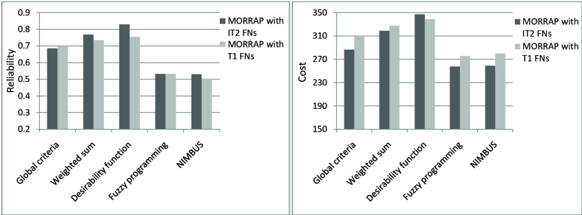
Figure 4: Comparative result of MORRAP with IT2 FNs and T1 FNs

Table 8: Solution of MORRAP with IT2 FNs and T1 FNs

	MORRAP with IT2 FNs	MORRAP with T1 FNs
Individual optimal value	Max $R_{s}=0.8317749$,	Max $R_{s}=0.8241383$,
	Min $C_{s}=181.2395$	Min $C_{s}=203.9562$
Multi-objective Method	Compromise solution	Compromise solution
Global criteria ($p=2$)	$R_{s}=0.6846485$, $C_{s}=286.5739$,	$R_{s}=0.6974577$, $C_{s}=309.8418$,
	$n_{1}=5$, $n_{2}=3$, $n_{3}=3$, $n_{4}=3$, $n_{5}=3$,	$n_{1}=5$, $n_{2}=3$, $n_{3}=3$, $n_{4}=3$, $n_{5}=3$,
	$n_{6}=2$, $n_{7}=2$, $n_{8}=2$, $n_{9}=2$, $n_{10}=1$.	$n_{6}=2$, $n_{7}=2$, $n_{8}=2$, $n_{9}=2$, $n_{10}=1$.
Weighted sum	$R_{s}=0.7683246$, $C_{s}=318.8198$,	$R_{s}=0.7349505$, $C_{s}=327.4596$,
	$n_{1}=5$, $n_{2}=3$, $n_{3}=3$, $n_{4}=3$, $n_{5}=3$,	$n_{1}=4$, $n_{2}=4$, $n_{3}=3$, $n_{4}=3$, $n_{5}=3$,
(with equal weights)	$n_{6}=2$, $n_{7}=2$, $n_{8}=2$, $n_{9}=2$, $n_{10}=2$.	$n_{6}=3$, $n_{7}=2$, $n_{8}=2$, $n_{9}=2$, $n_{10}=1$.
Desirability function	$R_{s}=0.829084$, $C_{s}=346.9919$,	$R_{s}=0.7542184$, $C_{s}=338.6593$,
$(t_{1}=1,t_{2}=0.1,$	$n_{1}=4$, $n_{2}=3$, $n_{3}=4$, $n_{4}=3$, $n_{5}=3$,	$n_{1}=4$, $n_{2}=4$, $n_{3}=3$, $n_{4}=3$, $n_{5}=3$,
$w_{1}=w_{2})$	$n_{6}=3$, $n_{7}=3$, $n_{8}=2$, $n_{9}=2$, $n_{10}=2$.	$n_{6}=3$, $n_{7}=3$, $n_{8}=2$, $n_{9}=2$, $n_{10}=1$.
Fuzzy programming	$R_{s}=0.5319160$, $C_{s}=257.5089$,	$R_{s}=0.5321748$, $C_{s}=275.6192$,
	$n_{1}=5$, $n_{2}=3$, $n_{3}=3$, $n_{4}=2$, $n_{5}=2$,	$n_{1}=4$, $n_{2}=3$, $n_{3}=2$, $n_{4}=2$, $n_{5}=3$,
	$n_{6}=2$, $n_{7}=2$, $n_{8}=1$, $n_{9}=2$, $n_{10}=1$.	$n_{6}=2$, $n_{7}=2$, $n_{8}=2$, $n_{9}=1$, $n_{10}=1$.
NIMBUS	$R_{s}=0.5306198$, $C_{s}=258.901$,	$R_{s}=0.5040566$, $C_{s}=280.0497$,
	$n_{1}=4$, $n_{2}=3$, $n_{3}=3$, $n_{4}=2$, $n_{5}=2$,	$n_{1}=4$, $n_{2}=3$, $n_{3}=3$, $n_{4}=3$, $n_{5}=4$,
	$n_{6}=2$, $n_{7}=2$, $n_{8}=2$, $n_{9}=1$, $n_{10}=1$.	$n_{6}=1$, $n_{7}=2$, $n_{8}=2$, $n_{9}=1$, $n_{10}=1$.

7 Conclusion

In this paper, we consider a multi-objective reliability-redundancy allocation problem (MORRAP) of a series-parallel system. Here, system reliability has to be maximized, and system cost has to be minimized simultaneously subject to limits on weight, volume, and redundancy level. Use of redundant components is commonly adapted approach to increase reliability of a system. However, incorporation of more redundant components may increase the cost of the system, for which optimal redundancy is mainly concerned for the economical design of system. Also, the component reliabilities in a system cannot always be precisely measured as crisp values, but may be determined as approximate values or approximate intervals with imprecise endpoints. To deal with impreciseness, the presented problem is formulated with the component reliabilities represented as IT2 FNs which are more flexible and appropriate to model impreciseness over usual or T1 FNs.

To solve MORRAP with interval type-2 fuzzy parameters, we first apply various type-reduction and corresponding defuzzification techniques, and obtain corresponding defuzzified values to observe the effect of different type-reduction strategies. We illustrate the problem with a real-world MORRAP on pharmaceutical plant. The objectives of the problem are conflicting with each other, and so one can obtain compromise solution in the sense that individual optimal solution can not be reached together. To deal with this, we apply five different multi-objective optimization techniques in the view that different results in hand give more flexibility to a decision maker to choose appropriate result according to his/her preference or as situation demand. We also solve the MORRAP with the uncertain (imprecise) component reliabilities represented as T1 FNs, and observe that modeling impreciseness using IT2 FNs leads to better performance than that of using T1 FNs. The present investigation has been done by modeling impreciseness using IT2 FNs. Therefore the present study can be extended by representing impreciseness using general T2 FNs. Also, we have used conventional multi-objective optimization techniques to deal with conflicting objectives. So it is also a matter of further investigation to deal with multiple objectives of the problem using evolutionary algorithms like Multi-Objective Genetic Algorithm (MOGA) and Non-dominated Sorting Genetic Algorithm (NSGA).

Acknowledgements:

The authors are thankful to the Editor and the anonymous Reviewers for valuable suggestions which lead to an improved version of the manuscript.

References

- Akalin et al. (2010) Akalin, O., Akay, K.U., Sennaroglu, B., Tez, M. (2010). Optimization of chemical admixture for concrete on mortar performance tests using mixture experiments. Chemometrics and Intelligent Laboratory Systems, 104, 233-242.
- Ardakan and Rezvan (2018) Ardakan, M.A., Rezvan, M.T. (2018). Multi-objective optimization of reliability redundancy allocation problem with cold-standby strategy using NSGA-II. Reliability Engineering & System Safety, 172, 225-238.
- Aliev and Kara (2004) Aliev, I.M., Kara, Z. (2004). Fuzzy system reliability analysis using time dependent fuzzy set. Control and Cybernetics, 33(4), 653-662.
- Bit et al. (1993) Bit, A.K., Biswal M.P., Alam, S.S. (1993). Fuzzy programming approach to multi-objective solid transportation problem. Fuzzy Sets and Systems, 57, 183-194.
- Caserta and Voß (2015) Caserta, M., Voß, S. (2015). An exact algorithm for the reliability redundancy allocation problem. European Journal of Operational Research, 244(1), 110-116.
- Cao et al. (2013) Cao, D., Murat, A., Chinnam, R.B. (2013). Efficient exact optimization of multi-objective redundancy allocation problems in series-parallel systems. Reliability Engineering and System Safety, 111, 154-163.
- Chen (1994) Chen, S.M. (1994). Fuzzy system reliability analysis using fuzzy number arithmetic operations. Fuzzy Sets and Systems, 64, 31-38.
- Cheng and Mon (2008) Cheng, C.H., Mon, D.L. (1993). Fuzzy system reliability analysis by interval of confidence. Fuzzy Sets and Systems, 56, 29-35.
- Coupland and John (2007) Coupland, S., John, R. (2007). Geometric type-1 and type-2 fuzzy logic systems, IEEE Transactions on Fuzzy Systems, 15(1), 3-15.
- Garg et al. (2014) Garg, H., Rani, M., Sharma, S.P., Vishwakarma, Y. (2014). Intuitionistic fuzzy optimization technique for solving multi-objective reliability optimization problems in interval environment. Expert Systems with Applications, 41(7), 3157-3167.
- Garg et al. (2013) Garg, H., Rani, M., Sharma, S.P. (2013). Reliability analysis of the engineering systems using intuitionistic fuzzy set theory. Journal of Quality and Reliability Engineering, 2013, Article ID 943972, 1-10.
- Garg and Sharma (2013) Garg H., Sharma, S.P. (2013). Multi-objective reliability-redundancy allocation problem using particle swarm optimization. Computers & Industrial Engineering, 64, 247-255.
- Hesamian (2017) Hesamian, G. (2017). Measuring similarity and ordering based on interval type 2 fuzzy numbers. IEEE Transactions on Fuzzy Systems, 25(4), 788-798.
- Huang et al. (2009) Huang, H-Z., Qu, J., Zuo, M.J. (2009). Genetic-algorithm-based optimal apportionment of reliability and redundancy under multiple objectives. IIE Transactions, 41(4), 287-298.
- Jamkhaneh and Nozari (2012) Jamkhaneh, E.B., Nozari, A. (2012). Fuzzy system reliability analysis based on confidence interval. Advanced Materials Research, 433-440, 4908-4914.
- Karnik and Mendel (2001) Karnik, N.N., Mendel, J.M. (2001). Centroid of a type-2 fuzzy set. Information Sciences, 132(1-4), 195-220.
- Khalili-Damghani et al. (2013) Khalili-Damghani, K., Abtahi, A.-R., Tavana, M. (2013). A new multi-objective particle swarm optimization method for solving reliability redundancy allocation problems. Reliability Engineering and System Safety, 111, 58-75.
- Kumar and Yadav (2012) Kumar, M., Yadav, S. P. (2012). A novel approach for analyzing fuzzy system reliability using different types of intuitionistic fuzzy failure rates of components. ISA Transactions, 51(2), 288-297.
- Kundu et al. (2014) Kundu, P., Kar, S., Maiti, M. (2014). Multi-objective solid transportation problems with budget constraint in uncertain environment. International Journal of Systems Science, 45(8), 1668-1682.
- Kuo and Prasad (2000) Kuo, W., Prasad, V.R. (2000). An annotated overview of system-reliability optimization. IEEE Transaction on Reliability, 49(2), 176-187.
- Liu (2008) Liu F. (2008). An efficient centroid type-reduction strategy for general type-2 fuzzy logic system. Information Sciences, 178, 2224-2236.
- Liu and Mendel (2008) Liu, F., Mendel, J.M. (2008). Encoding words into interval type-2 fuzzy sets using an interval approach. IEEE Transactions on Fuzzy Systems, 16(6), 1503-1521.
- Mahapatra and Roy (2006) Mahapatra, G.S., Roy, T.K. (2006). Fuzzy multi-objective mathematical programming on reliability optimization model. Applied Mathematics and Computation, 174, 643-659.
- Malenović et al. (2011) Malenović, A., Dotsikas, Y., Mašković, M., Jančić-Stojanović, B., Ivanović, D., Medenica, M. (2011). Desirability-based optimization and its sensitivity analysis for the perindopril and its impurities analysis in a microemulsion LC system. Microchemical Journal, 99, 454-460.
- Mendel (2003) Mendel, J.M. (2003). Fuzzy sets for words: a new beginning. Proceedings of IEEE International Conference on Fuzzy Systems, 37-42, St. Louis, MO.
- Mendel (2007a) Mendel, J.M. (2007a). Computing with words: Zadeh, Turing, Popper and Occam. IEEE Computational Intelligence Magazine, 2(4), 10 17.
- Mendel (2007b) Mendel, J.M. (2007b). Computing with words and its relationships with fuzzistics. Information Sciences, 177, 988-1006.
- Mendel and John (2002) Mendel, J.M., John, R.I. (2002). Type-2 fuzzy sets made simple. IEEE Transactions on Fuzzy Systems, 10(2), 307-315.
- Mendel et al. (2006) Mendel, J. M., John, R.I., Liu, F.L. (2006). Interval type-2 fuzzy logical systems made simple. IEEE Transactions on Fuzzy Systems, 14(6), 808-821.
- Mendel and Liu (2007) Mendel, J.M., Liu, F. (2007). Super-exponential convergence of the Karnik-Mendel algorithms for computing the centroid of an interval type-2 fuzzy set. IEEE Transaction on Fuzzy Systems, 15(2), 309-320.
- Mendel and Wu (2006) Mendel, J.M., Wu, H. (2006). Type-2 fuzzistics for symmetric interval type-2 fuzzy sets: Part 1, forward problems. IEEE Transactions on Fuzzy Systems, 14(6), 781-792.
- Miller et al. (2012) Miller, S., Gongora, M., Garibaldi, J., John, R. (2012). Interval type-2 fuzzy modelling and stochastic search for real-world inventory management. Soft Computing, 16, 1447-1459.
- Miettinen (2012) Miettinen, K. (2012). Nonlinear Multiobjective Optimization. Springer Science & Business Media, US.