GHFP: Gradually Hard Filter Pruning

Abstract

Filter pruning is widely used to reduce the computation of deep learning, enabling the deployment of Deep Neural Networks (DNNs) in resource-limited devices. Conventional Hard Filter Pruning (HFP) method zeroizes pruned filters and stops updating them, thus reducing the search space of the model. On the contrary, Soft Filter Pruning (SFP) simply zeroizes pruned filters, keeping updating them in the following training epochs, thus maintaining the capacity of the network. However, SFP, together with its variants, converges much slower than HFP due to its larger search space. Our question is whether SFP-based methods and HFP can be combined to achieve better performance and speed up convergence. Firstly, we generalize SFP-based methods and HFP to analyze their characteristics. Then we propose a Gradually Hard Filter Pruning (GHFP) method to smoothly switch from SFP-based methods to HFP during training and pruning, thus maintaining a large search space at first, gradually reducing the capacity of the model to ensure a moderate convergence speed. Experimental results on CIFAR-10/100 show that our method achieves the state-of-the-art performance.

Index Terms—  Filter Pruning, Network Compression, Neural Network, and Classification.

1 Introduction

Despite the success of deep Convolutional Neural Networks (CNNs) in visual tasks from image classification [1, 2] to object detection [3], their expensive computation cost and memory footprint hinder their deployment in resource-limited devices. Thus, it is necessary to compress DNN models with little loss in performance.

A typical filter pruning pipeline is composed of four phases: training a network, evaluating the importance of every filter, pruning unimportant filters and fine-tuning. The fine-tuning phase is to compensate for the performance loss caused by pruning. Prevalent filter pruning methods can be divided into two categories: hard filter pruning (HFP) and soft filter pruning (SFP) [4]. While SFP zeroizes pruned filters and updates them in the following training epochs to maintaining the capacity of the network, HFP would not update those pruned filters any more.

A disadvantage of SFP is that there will be a severe accuracy drop after pruning when the pruning rate is large due to its large search space. There are three variants of SFP to alleviate this issue, named SofteR Filter Pruning (SRFP) [5], Asymptotic Soft Filter Pruning (ASFP) [6] and Asymptotic SofteR Filter Pruning (ASRFP) [5] respectively. ASFP gradually increases the pruning rate from zero to the final pruning rate to alleviate the accuracy drop caused by pruning, while SRFP decays the pruned weights with a monotonic decreasing parameter to soften the effect of pruning. ASRFP is a combination of ASFP and SRFP to simultaneously increase the pruning rate and use a decreasing parameter. For clarity, we use ASP to denote ASFP and ASRFP.

However, these soft pruning methods could not avoid this severe accuracy drop because they maintain a large search space, while HFP would gradually reduce the capacity of the model to ensure convergence. As shown in Figure 1, while for small pruning rates like 0.2, ASP may outperform HFP, for large pruning rates like 0.8, HFP is more advantageous. Specifically, for small pruning rates, the overall trend of the test accuracy is downward as the ratio of HFP increases from 0 to 1, meaning that ASP may be superior to HFP for small pruning rates, while the overall trend is upward for large pruning rates.

Thus, we propose a Gradually Hard Filter Pruning (GHFP) method to smoothly switch from ASP to HFP during training and pruning to achieve a balance between performance and convergence speed, as shown in Figure 2. We utilize a monotonic increasing parameter to control the ratio of HFP, increasing from 0 to 1, thus acting like ASP to maintain a large capacity at start, gradually increasing the rate of HFP to reduce the search space to ensure convergence.

Our contributions are as follows: (1) We generalize ASP and HFP to analyze their characteristics, noting that ASP maintains a large search space at the cost of much slower convergence speed than that of HFP. (2) We propose GHFP to smoothly switch from ASP to HFP during training and pruning, performing well across various networks, datasets and pruning rates. (3) We find that HFP is still a reliable choice for large pruning rates.

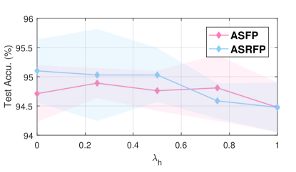
(a) Pruning Rate = 0.2

(b) Pruning Rate = 0.8

Fig. 1: Comparison of CIFAR-10 test accuracies of different $\lambda_{h}$ and pruning rates for ResNet-110, where $\lambda_{h}$ is the ratio of HFP to the total pruning rate. $\lambda_{h}=0$ means pure ASP, while $\lambda_{h}=1$ means pure HFP. (Solid line and shadow represent the mean and standard deviation respectively.)

2 Related works

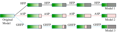
Fig. 2: Overview of our GHFP method. We use ”ASP” to denote ASFP and ASRFP as they belong to the general soft filter pruning and they gradually increase the pruning rate from zero to the final pruning rate as HFP does. Green, gray and pink rectangles represent unpruned filters, hard pruned filters and softly pruned filters respectively. Deeper Green means more important filters. Softly pruned filters are allowed to update their parameters in the following training epochs, while hard pruned filters are not. Thus, ASP maintains a large search space, having trouble in obtaining a really compact model as HFP, which gradually reduces the search space to ensure convergence. Our GHFP uses a monotonic increasing parameter to control the ratio of HFP, increasing from 0 to 1 to balance performance and convergence speed.

Previous works on accelerating CNNs mainly consist of matrix decomposition [7, 8], quantization [9], fast convolution [10, 11, 12], knowledge distillation [13] and pruning.

Pruning-based methods focus on removing unimportant connections or neurons to compress and accelerate the network. Pruning methods can be divided into two categories: weight pruning and filter pruning. Weight pruning methods compress networks in an unstructured manner by deleting redundant weights, thus inducing sparsity in filters. While weight pruning methods require specialized libraries to obtain real acceleration, filter pruning directly deletes unimportant filters in a structured manner, capable of easily reducing both the model size and the computational overhead [14, 15, 16, 24].

During these years, numerous filter pruning methods have been proposed. Prevalent criteria for measuring the importance of a filter or a channel include $\ell_{1}$-norm, $\ell_{2}$-norm, scaling factors, feature redundancy and cross-layer filter comparison [17, 18, 19, 20]. Recently proposed Filter Pruning via Geometric Median (FPGM) method indicates that the widely used “smaller-norm-less-important” criterion requires significant deviation of filter norms and norms of those filters chosen to be pruned close to zeros, and proposes to prune filters via Geometric Median [21], while Guided Structured Sparsity (GSS) imposes group sparsity and group variance losses to force a portion of neurons in each layer to stay alive [22]. In effect, GSS pushes filters to have a high variance with a concentration around zero, which is consistent with the requirements of “smaller-norm-less-important” criterion unintentionally.

SFP and ASFP simply set pruned filters to zeros during training, keeping updating them in the following training epochs to maintain a large search space. In contrast, SRFP and ASRFP decay pruned filters with a monotonic decreasing parameter in order to alleviate the information loss caused by pruning. Nevertheless, although maintaining a large search space, these soft pruning methods converge much slower than HFP in case of large pruning rates.

Hence, we propose a Gradually Hard Filter Pruning (GHFP) method to smoothly switch from ASP to HFP during training and pruning to strike a balance between performance and convergence speed. We utilize a monotonic increasing parameter to control the ratio of HFP, increasing from 0 to 1, initially acting like ASP to maintain a large search space, gradually increasing the rate of HFP to reduce the search space to ensure convergence.

3 Our method

3.1 Formulation

The dimension of the convolutional kernel in the $i$-th layer ${W}_{i}$ can be denoted as $n\times m\times s\times s$, where $1\leq i\leq L$ and $L$ is the total number of convolutional layers in a network. Concretely, $s$ denotes the kernel size. $m$ and $n$ represent the number of input channels and output channels respectively.

The shape of the input tensor ${I}_{i}$ is $m\times h_{i}\times w_{i}$ and the output tensor ${O}_{i}\in\mathbb{R}^{n\times h_{i+1}\times w_{i+1}}={W}_{i}\ast{I}_{i}$ can be written as

$${O}_{i,j}={W}_{i,j}\ast{I}_{i}~{} ~{}{for}~{}1\leq j\leq n,$$ (1)

where ${O}_{i,j}\in\mathbb{R}^{h_{i+1}\times w_{i+1}}$ is the $j$-th output channel in the $i$-th layer and ${W}_{i,j}\in\mathbb{R}^{m\times s\times s}$ denotes the $j$-th filter in the $i$-th layer.

Assume the filter pruning rate for the $i$-th layer to be $P_{i}$. Hence, we will delete $n\times P_{i}$ filters in the $i$-th layer, and the shape of the pruned output tensor ${O}_{i}$ is ${n\times(1-P_{i})\times h_{i+1}\times w_{i+1}}$.

Soft Pruning. Based on the SRFP method and its variant ASRFP, the pruned weights of the $i$-th layer are simply zeroized, which can be represented by

$${\hat{W}}_{i,j}\!=\!{W}_{i,j}\!\odot\!{M}_{i,j}\!+\!\alpha\;\!{W}_{i,j}\!\odot\!(1\!-\!{M}_{i,j})~{} ~{}{for}~{}1\leq j\leq n,$$ (2)

where ${M}_{i,j}$ is a Boolean mask of the filter ${W}_{i,j}$ to represent whether the $j$-th filter in the $i$-th layer is removed. $\hat{W}_{i,j}$ is the resulted filter. ${M}_{i,j}=0$ if ${W}_{i,j}$ is pruned. Otherwise, ${M}_{i,j}=1$ denotes that the filter ${W}_{i,j}$ is not pruned. $\odot$ denotes the element-wise multiplication. $\alpha$ is a monotonic decreasing parameter to control the decaying speed of pruned filters and to better utilize the trained information of pruned filters. Generally, $\alpha\in[0,1]$. SFP and ASFP are special cases of SRFP and ASRFP respectively when $\alpha=0$.

When $\alpha\in(0,1]$, the trained information of pruned filters is not entirely abandoned. Nevertheless, when $\alpha>0$, the softly pruned model is not compact, since pruned filters are not zeroized. Hence, SRFP and ASRFP gradually decay $\alpha$ from 1 towards 0 via an exponential decay strategy, given by

$$\alpha_{e}(t)=\alpha_{0}(\frac{\alpha_{0}}{\epsilon})^{-\frac{t}{t_{max}-1}}~{} ~{}{for}~{}0\leq t<t_{max},$$ (3)

where $t_{max}$ is the maximal number of training epochs and $\alpha_{0}=1$ in SRFP and ASRFP. $\epsilon$ is infinitely close to zero to satisfy that

$$\alpha_{e}(t_{max}-1)=\epsilon\to 0.~{}$$ (4)

When $\alpha_{e}(t)$ is close to zero enough, SRFP and ASRFP set $\alpha_{e}(t)=0$ to obtain a really compact model.

Hard Pruning. In HFP, the pruning rate, consistent with that of ASRFP, would gradually increase from 0 to the final pruning rate. Therefore, HFP can be seen as a special case of ASRFP when $\alpha=0$, apart from stopping updating pruned filters, represented as

$${\hat{G}}_{i,j}\!=\!{G}_{i,j}\!\odot\!{M}_{i,j}~{} ~{}{for}~{}1\leq j\leq n,$$ (5)

where ${G}_{i,j}$ is the gradient of the filter ${W}_{i,j}$ and $\hat{G}_{i,j}$ is the masked gradient. Only unpruned filters could update their weights. Thus, for one thing, the representative capacity of the model is gradually reduced. For another, the search space is gradually narrowed to ensure convergence.

3.2 Gradually Hard Filter Pruning (GHFP)

Although maintaining a large search space, soft pruning methods converge much slower than HFP in case of large pruning rates.

Therefore, we propose a Gradually Hard Filter Pruning (GHFP) method to smoothly switch from ASP to HFP during training and pruning to achieve a balance between performance and convergence speed. We adopt a monotonic increasing parameter $\lambda_{h}$ to control the ratio of HFP, increasing from 0 to 1, given by

$$\lambda_{h}(t)\!=\!\lambda_{i}\!+\!(\lambda_{f}\!-\!\lambda_{i})\!\left[\!1\!\!-\!\!(\frac{\!t_{max}\!-\!1\!-\!t}{t_{max-1}})^{3}\!\right]\!\!\!~{} ~{}\!{for}~{}0\!\leq t\!<\!t_{max},$$ (6)

where $\lambda_{i}$ and $\lambda_{f}$ are the initial and final ratio of HFP respectively. If the pruning rate of the $i$-th layer in the $t$-th epoch is $P_{i}(t)$, we simply set $P_{i}(t)\times n$ channels to zeros, among which $\lambda_{h}(t)\times P_{i}(t)\times n$ channels with minimum $\ell_{2}$-norms are pruned in a hard manner, while $(1-\lambda_{h}(t))\times P_{i}(t)\times n$ channels are softly pruned, where $n$ is the number of channels in the $i$-th layer.

We simply set $\lambda_{i}=0$, $\lambda_{f}=1$ and $t_{max}=200$. Thus, as shown in Figure 3, our GHFP initially acts like ASP to maintain a large capacity, gradually increasing the rate of HFP to reduce the search space to ensure convergence. We present our GHFP method in Algorithm 1. Especially, if $\alpha_{0}=0$, we called our method ASFP combined with HFP. Otherwise, we called it ASRFP combined with HFP.

inputs : training set: ${X}$, final pruning rate: $P_{i}$, initial decay rate: $\alpha_{0}$, the model with parameters ${W}=\{{W}_{i},0\leq i\leq L\}$.

output : The pruned model with parameters ${W}^{*}={W}^{t_{max}}$

Initialize the model parameter ${W}^{0}$

Initialize HFP rate $\lambda_{h}(0)=0$

Initialize Pruning rate $P_{i}(0)=0$

for $t=0$, …, $t_{max}-1$ do

       Decrease weight decay rate $\alpha$ with Eq.(3)

       Increase HFP rate $\lambda_{h}(t)$ with Eq.(6)

       Increase pruning rate $P_{i}(t)$ based on ASFP

       Train model parameters $\hat{W}^{t+1}$ based on data set ${X}$ and ${W}^{t}$

       for $i=1$, …, $L$ do

             Compute the $\ell_{2}$-norm of each filter $\|\hat{W}_{i,j}^{t+1}\|_{2},1\leq j\leq n$

             Select $n\times P_{i}$ filters with minimal $\ell_{2}$-norm values

             $\lambda_{h}(t)\times P_{i}(t)\times n$ filters with minimum $\ell_{2}$-norms are pruned hard

             $(1-\lambda_{h}(t))\times P_{i}(t)\times n$ remaining chosen filters are softly pruned using $\alpha$

            

      Get the pruned model parameters ${W}^{t+1}$ based on $\hat{W}^{t+1}$

Get the pruned model with final parameters ${W}^{*}={W}^{t_{max}}$

Algorithm 1 GHFP Algorithm

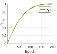
Fig. 3: Gradually increase the proportion of HFP as the training and pruning procedure goes on.

4 Experiments

4.1 Setup

Our method is evaluated on CIFAR-10/100 [23]. CIFAR-10 and CIFAR-100 include 50,000 training images and 10,000 test images of size $32\times 32$ pixels, divided into 10 and 100 classes respectively. We mainly prune the challenging ResNet, following the experimental setup in CP [25], ASFP [6]. We also prune the VGG-16 [26] following the setup in [17, 18, 6].

On CIFAR-10/100, we follow the parameter scheme and the training configuration in [27, 6].

Our GHFP is adopted after each training epoch. Models are trained from scratch by default. Results starting from pre-trained models are also provided, where the learning rate is one tenth of that of models trained from scratch. Experiments are repeated four times. Then we compare our results with other state-of-the-art methods, e.g., SFP [4], SRFP [5], ASRFP [5], ASFP [6], MIL [28], PFEC [17], CP [25], FPGM [21], VCNNP [29].

4.2 Results on CIFAR-10

Settings. On CIFAR-10, our GHFP is evaluated on VGG-16 and ResNet-20/56/110.

Results. We summarize the results on CIFAR-10 in Table 1, Table 2 and Table 3, where ”Our1” and ”Our2” denote ASFP combined with HFP and ASRFP combined with HFP respectively. ”PR” means the pruning rate. Models are trained from scratch by default. Both GHFP methods achieve competitive performance on CIFAR-10 compared with other channel pruning methods across networks of various depths and pruning rates. Particularly, ASFP combined with HFP outperforms other methods in most cases, while the performance of ASRFP combined with HFP fluctuates obviously.

Table 1: Pruning results of ResNet-20/110 on CIFAR-10.

Depth	Method	Baseline(%)	Accu.(%)	FLOPs(PR%)
20	MIL [28]	91.53	91.43	3.20E7(20.3)
	SFP(20%)	92.32	91.40	2.87E7(29.3)
	SRFP(20%)	92.32	91.47	2.87E7(29.3)
	ASFP(20%)	92.89	91.62	2.87E7(29.3)
	ASRFP(20%)	92.89	91.67	2.87E7(29.3)
	Our1(20%)	92.89	92.14	2.87E7(29.3)
	Our2(20%)	92.89	92.41	2.87E7(29.3)
	ASFP(40%)	92.89	90.57	2.43E7(54.0)
	ASRFP(40%)	92.89	90.65	2.43E7(54.0)
	Our1(40%)	92.89	90.82	2.43E7(54.0)
	Our2(40%)	92.89	91.28	2.43E7(54.0)
110	PFEC [17]	93.53	92.94	1.55E8(38.6)
	MIL [28]	93.63	93.44	-(34.2)
	SFP(20%)	94.33	93.86	1.82E8(28.2)
	SRFP(20%)	94.33	93.61	1.82E8(28.2)
	ASFP(20%)	94.76	94.71	1.82E8(28.2)
	ASRFP(20%)	94.76	95.10	1.82E8(28.2)
	Our1(20%)	94.76	95.16	1.82E8(28.2)
	Our2(20%)	94.76	94.59	1.82E8(28.2)

Table 2: Pruning results of ResNet-56 on CIFAR-10. ${\star}$ denotes pruning from pre-trained models.

Method	Baseline(%)	Accu.(%)	FLOPs(PR%)
PFEC [17]	93.04	91.31	9.09E7(27.6)
CP [25]	92.80	90.90	-(50.0)
SFP(20%)	93.66	93.26	8.98E7(28.4)
SRFP(20%)	93.66	93.33	8.98E7(28.4)
ASFP(20%)	94.85	93.97	8.98E7(28.4)
ASRFP(20%)	94.85	93.77	8.98E7(28.4)
Our1(20%)	94.85	94.17	8.98E7(28.4)
Our2(20%)	94.85	94.10	8.98E7(28.4)
PFEC⋆ [17]	93.04	93.06	9.09E7(27.6)
SFP(20%)⋆	93.66	93.25	8.98E7(28.4)
ASFP(20%)⋆	94.85	94.92	8.98E7(28.4)
ASRFP(20%)⋆	94.85	94.98	8.98E7(28.4)
Our1(20%)⋆	94.85	95.07	8.98E7(28.4)
Our2(20%)⋆	94.85	94.92	8.98E7(28.4)
ASFP(40%)	94.85	93.64	5.94E7(52.6)
ASRFP(40%)	94.85	93.68	5.94E7(52.6)
Our1(40%)	94.85	93.84	5.94E7(52.6)
Our2(40%)	94.85	93.75	5.94E7(52.6)
ASFP(60%)⋆	94.85	89.72	3.43E7(72.6)
ASRFP(60%)⋆	94.85	90.54	3.43E7(72.6)
Our1(60%)⋆	94.85	92.54	3.43E7(72.6)
Our2(60%)⋆	94.85	93.00	3.43E7(72.6)

Table 3: Pruning results of VGG-16 on CIFAR-10. ${\star}$ denotes pruning from pre-trained models.

Method	Baseline(%)	Accu.(%)	FLOPs (PR%)
PFEC [17]	93.58	93.31	2.04E8(34.2)
FPGM [21]	93.58	93.23	1.99E8(35.9)
VCNNP [29]	93.25	93.18	1.90E8(39.1)
SFP(20%)	93.62	93.11	2.04E8(34.2)
Our1(20%)	93.62	93.34	2.04E8(34.2)
Our2(20%)	93.62	93.29	2.04E8(34.2)
PFEC⋆ [17]	93.58	93.28	2.04E8(34.2)
SFP(20%)⋆	93.62	93.69	2.04E8(34.2)
ASFP(20%)⋆	93.62	93.75	2.04E8(34.2)
ASRFP(20%)⋆	93.62	93.76	2.04E8(34.2)
Our1(20%)⋆	93.62	93.96	2.04E8(34.2)
Our2(20%)⋆	93.62	93.76	2.04E8(34.2)

4.3 Results on CIFAR-100

Settings. On CIFAR-100, our GHFP is evaluated on ResNet-20/56/110.

Results. We conclude the results on CIFAR-100 in Table 4, where ”Our1” and ”Our2” denote ASFP combined with HFP and ASRFP combined with HFP respectively. Both GHFP methods still achieve competitive performance. Especially, ASRFP combined with HFP obviously outperforms other methods on CIFAR-100.

Table 4: Pruning results of ResNet-20/56/110 on CIFAR-100.

Depth	Method	Baseline(%)	Accu.(%)	FLOPs(PR%)
20	SFP(20%)	68.11	66.23	2.87E7(29.3)
	SRFP(20%)	68.11	66.67	2.87E7(29.3)
	ASFP(20%)	68.92	66.95	2.87E7(29.3)
	ASRFP(20%)	68.92	66.48	2.87E7(29.3)
	Our1(20%)	68.92	66.85	2.87E7(29.3)
	Our2(20%)	68.92	67.62	2.87E7(29.3)
56	SFP(20%)	72.00	70.49	8.98E7(28.4)
	SRFP(20%)	72.00	70.39	8.98E7(28.4)
	ASFP(20%)	72.92	71.01	8.98E7(28.4)
	ASRFP(20%)	72.92	71.24	8.98E7(28.4)
	Our1(20%)	72.92	71.46	8.98E7(28.4)
	Our2(20%)	72.92	71.93	8.98E7(28.4)
110	SFP(20%)	73.85	72.66	1.82E8(28.2)
	SRFP(20%)	73.85	73.00	1.82E8(28.2)
	ASFP(20%)	74.39	72.91	1.82E8(28.2)
	ASRFP(20%)	74.39	73.02	1.82E8(28.2)
	Our1(20%)	74.39	72.95	1.82E8(28.2)
	Our2(20%)	74.39	73.29	1.82E8(28.2)

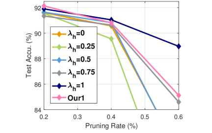
(a) ASFP combined with HFP

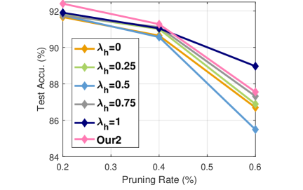
(b) ASRFP combined with HFP

Fig. 4: Comparison of different $\lambda_{h}$ for ResNet-20 on CIFAR-10 among ”Soft and Hard”, ASFP combined with HFP(denoted by ”Our1”) and ASRFP combined with HFP(denoted by ”Our2”). $\lambda_{h}=1$ exactly means HFP while $\lambda_{h}=0$ exactly means ASP.

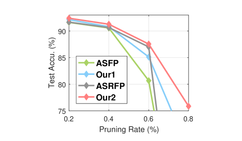
(a) ResNet-20

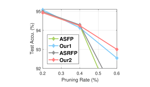
(b) ResNet-56

Fig. 5: Comparison of test accuracies of different pruning rates for ResNet-20/56 on CIFAR-10 among ASFP, ASRFP, ASFP combined with HFP(denoted by ”Our1”) and ASRFP combined with HFP(denoted by ”Our2”).

4.4 Ablation study

Extensive ablation experiments of are conducted to analyze our GHFP.

Soft and Hard v.s. Soft to Hard. We compare results of using a constant $\lambda_{h}$ during training, named ”Soft and Hard” and our GHFP, called ”Soft to Hard”, because a constant $\lambda_{h}\in(0,1)$ makes some filters hard pruned and some filters pruned softly. As shown in Figure 4(a) and Figure 4(b), GHFP-based methods, ASFP combined with HFP and ASRFP combined with HFP outperform ”Soft and Hard” methods in terms of performance and stability. Besides, even though our GHFP outperforms soft filter pruning methods, HFP is still a remarkable choice in case of large pruning rates. Our GHFP is more likely to achieve better performance in case of small pruning rates.

Varying pruning rates. To further investigate the efficacy of our GHFP method, we present test accuracies of different pruning rates for ResNet-20/56 in Figure 5(a) and Figure 5(b), where ResNet-20 is trained from scratch and ResNet-56 is trained from a pre-trained model. As the pruning rate increases, the test accuracies of GHFP-based methods decline much steadier than those of ASFP and ASRFP. In both cases, our GHFP-based methods outperform ASFP and ASRFP in terms of stability and test accuracy across diverse pruning rates.

5 Conclusions

We analyze the characteristics of soft pruning methods and HFP, noting that although pursuing better performance, soft pruning methods may be confronted with severe test accuracy drops in case of large pruning rates because they don’t reduce their search space to ensure convergence. Hence, we propose a method named GHFP to smoothly switch from ASP to HFP during training and pruning to achieve a balance between performance and convergence speed. Our GHFP performs well across various networks, datasets and pruning rates. Besides, HFP is a reliable choice for large pruning rates.

References

- [1] Kaiming He, Xiangyu Zhang, Shaoqing Ren, and Jian Sun, “Deep residual learning for image recognition,” Proceedings of the IEEE Computer Society Conference on Computer Vision and Pattern Recognition, vol. 2016-December, pp. 770–778, 2016.
- [2] Chuanguang Yang, Zhulin An, Hui Zhu, Xiaolong Hu, Kun Zhang, Kaiqiang Xu, Chao Li, and Yongjun Xu, “Gated convolutional networks with hybrid connectivity for image classification,” in The Thirty-Fourth AAAI Conference on Artificial Intelligence, AAAI 2020. 2020, pp. 12581–12588, AAAI Press.
- [3] Ross Girshick, Jeff Donahue, Trevor Darrell, and Jitendra Malik, “Rich feature hierarchies for accurate object detection and semantic segmentation,” in Proceedings of the IEEE Computer Society Conference on Computer Vision and Pattern Recognition, 2014.
- [4] Yang He, Guoliang Kang, Xuanyi Dong, Yanwei Fu, and Yi Yang, “Soft filter pruning for accelerating deep convolutional neural networks,” IJCAI International Joint Conference on Artificial Intelligence, vol. 2018-July, pp. 2234–2240, 2018.
- [5] Linhang Cai, Zhulin An, Chuanguang Yang, and Yongjun Xu, “Softer Pruning, Incremental Regularization,” Proceedings - International Conference on Pattern Recognition, 2020.
- [6] Yang He, Xuanyi Dong, Guoliang Kang, Yanwei Fu, Chenggang Yan, and Yi Yang, “Asymptotic Soft Filter Pruning for Deep Convolutional Neural Networks,” IEEE Transactions on Cybernetics, vol. PP, pp. 1–11, 2019.
- [7] Max Jaderberg, Andrea Vedaldi, and Andrew Zisserman, “Speeding up convolutional neural networks with low rank expansions,” in BMVC 2014 - Proceedings of the British Machine Vision Conference 2014, 2014.
- [8] Jose M. Alvarez and Mathieu Salzmann, “Compression-aware training of deep networks,” Advances in Neural Information Processing Systems, vol. 2017-December, no. Nips, pp. 857–868, 2017.
- [9] Itay Hubara, Matthieu Courbariaux, Daniel Soudry, Ran El-Yaniv, and Yoshua Bengio, “Binarized neural networks,” in Advances in Neural Information Processing Systems, 2016.
- [10] Alex Krizhevsky, Ilya Sutskever, and Geoffrey E. Hinton, “ImageNet classification with deep convolutional neural networks,” Advances in Neural Information Processing Systems, vol. 2, pp. 1097–1105, 2012.
- [11] Andrew G. Howard, Menglong Zhu, Bo Chen, Dmitry Kalenichenko, Weijun Wang, Tobias Weyand, Marco Andreetto, and Hartwig Adam, “MobileNets: Efficient Convolutional Neural Networks for Mobile Vision Applications,” 2017.
- [12] Pravendra Singh, Vinay Kumar Verma, Piyush Rai, and Vinay P. Namboodiri, “HetConv: Heterogeneous Kernel-Based Convolutions for Deep CNNs,” 2019.
- [13] Geoffrey Hinton, Oriol Vinyals, and Jeff Dean, “Distilling the Knowledge in a Neural Network,” pp. 1–9, 2015.
- [14] M. Zhu and S. Gupta, “To prune, or not to prune: exploring the efficacy of pruning for model compression,” ArXiv, vol. abs/1710.01878, 2018.
- [15] Zhuang Liu, M. Sun, Tinghui Zhou, Gao Huang, and Trevor Darrell, “Rethinking the value of network pruning,” ArXiv, vol. abs/1810.05270, 2019.
- [16] Jonathan Frankle and Michael Carbin, “The lottery ticket hypothesis: Finding sparse, trainable neural networks,” arXiv: Learning, 2019.
- [17] Hao Li, Asim Kadav, Igor Durdanovic, Hanan Samet, and Hans Peter Graf, “Pruning Filters for Efficient ConvNets,” , no. 2016, pp. 1–13, 2016.
- [18] Zhuang Liu, Jianguo Li, Zhiqiang Shen, Gao Huang, Shoumeng Yan, and Changshui Zhang, “Learning Efficient Convolutional Networks through Network Slimming,” Proceedings of the IEEE International Conference on Computer Vision, vol. 2017-Octob, pp. 2755–2763, 2017.
- [19] Babajide O. Ayinde and Jacek M. Zurada, “Building Efficient ConvNets using Redundant Feature Pruning,” pp. 1–9, 2018.
- [20] Wenxiao Wang, Cong Fu, Jishun Guo, Deng Cai, and Xiaofei He, “COP: Customized deep model compression via regularized correlation-based filter-level pruning,” in IJCAI International Joint Conference on Artificial Intelligence, 2019.
- [21] Yang He, Ping Liu, Ziwei Wang, Zhilan Hu, and Y. Yang, “Filter pruning via geometric median for deep convolutional neural networks acceleration,” 2019 IEEE/CVF Conference on Computer Vision and Pattern Recognition (CVPR), pp. 4335–4344, 2019.
- [22] A. Torfi and Rouzbeh A. Shirvani, “Attention-based guided structured sparsity of deep neural networks,” ArXiv, vol. abs/1802.09902, 2018.
- [23] Alex Krizhevsky, “Learning Multiple Layers of Features from Tiny Images,” … Science Department, University of Toronto, Tech. …, 2009.
- [24] Jian Hao Luo, Jianxin Wu, and Weiyao Lin, “ThiNet: A Filter Level Pruning Method for Deep Neural Network Compression,” Proceedings of the IEEE International Conference on Computer Vision, vol. 2017-Octob, pp. 5068–5076, 2017.
- [25] Yihui He, Xiangyu Zhang, and Jian Sun, “Channel Pruning for Accelerating Very Deep Neural Networks,” Proceedings of the IEEE International Conference on Computer Vision, vol. 2017-October, pp. 1398–1406, 2017.
- [26] Karen Simonyan and Andrew Zisserman, “Very deep convolutional networks for large-scale image recognition,” in 3rd International Conference on Learning Representations, ICLR 2015 - Conference Track Proceedings, 2015.
- [27] Kaiming He, Xiangyu Zhang, Shaoqing Ren, and Jian Sun, “Identity mappings in deep residual networks,” Lecture Notes in Computer Science (including subseries Lecture Notes in Artificial Intelligence and Lecture Notes in Bioinformatics), vol. 9908 LNCS, pp. 630–645, 2016.
- [28] Xuanyi Dong, Junshi Huang, Yi Yang, and Shuicheng Yan, “More is less: A more complicated network with less inference complexity,” in Proceedings - 30th IEEE Conference on Computer Vision and Pattern Recognition, CVPR 2017, 2017.
- [29] Chenglong Zhao, B. Ni, Jia yu Zhang, Qiwei Zhao, W. Zhang, and Q. Tian, “Variational convolutional neural network pruning,” 2019 IEEE/CVF Conference on Computer Vision and Pattern Recognition (CVPR), pp. 2775–2784, 2019.