Variational approach with the superposition of the symmetry-restored quasi-particle vacua for nuclear shell-model calculations

Abstract

We propose a variational calculation scheme utilizing the superposition of the angular-momentum, parity, number projected quasiparticle vacua, that is especially suitable for applying to medium-heavy nuclei in shell-model calculations. We derive a formula for the energy variance with quasi-particle vacua and apply the energy-variance extrapolation to the present scheme for further precise estimation of the exact shell-model energy. The validity of the method is presented for the shell-model calculation of ¹³²Ba in the $50\leq Z,N\leq 82$ model space. We also discuss the feasibility of this scheme in the case of the ¹⁵⁰Nd in the $50\leq Z\leq 82$ and $82\leq Z\leq 126$ model space and demonstrate that its neutrinoless-double-beta-decay matrix element is obtained showing good convergence.

I Introduction

Nuclear shell model calculation can describe any many-body correlations inside the valence shell on equal footing by configuration mixing and it is one of the most powerful tools to investigate the ground and low-lying excited states of nuclei caurier_rmp ; otsuka_rmp . However, the number of the configurations to be considered, namely the dimension of the shell-model Hamiltonian matrix, increases explosively depending on the model space and the number of the active particles, and thus it hampers the application of shell-model calculations to the medium-heavy nuclei strictly. Several shell-model codes have been developed for massively parallel computations to treat such a large-scale problem mfdn ; kshell ; bigstick . Despite these appreciable efforts, the application of the conventional shell-model calculation is restricted by the limitation of available computational resources. The current feasible $M$-scheme dimension of the Hamiltonian matrix is $O(10^{11})$, which implies that shell-model calculations are applicable only to near semi-magic nuclei in medium-heavy mass region.

In order to overcome this difficulty and to broaden the applicability of the configuration-mixing framework, a lot of efforts have been paid to develop various theoretical frameworks to obtain shell-model solutions where the conventional Lanczos diagonalization method cannot reach, such as the projected shell model proj_sm , the pair truncation npa ; yoshinaga_npa , the Monte Carlo shell model (MCSM) and its extension mcsm_ppnp ; mcsm_ptep , the VAMPIR approach and its variants vampir ; vampir_ppnp , the hybrid multi-determinant method puddu_hmd , the iterative diagonalization algorithm iter_diag , the correlated-basis method corr_sm , the density matrix renormalization group method dmrg_sm , the importance truncated shell model itsm_extrap , and the generator coordinate method (GCM) hfb_gcm . Recently, the GCM method has been introduced into the in-medium similarity renormalization group method to evaluate nuclear matrix elements for neutrinoless double-beta decay yao_gcm_srg_1 ; yao_gcm_srg_2 ; yao_gcm_srg_3 . Note that the auxiliary-field quantum Monte Carlo approach can be used to the configuration mixing approach, but the realistic shell-model Hamiltonian has the Fermion sign problem, which restricts its application to the practical shell-model calculation severely smmc ; smmc_gammasoft ; cp_smmc .

Among them, the MCSM is one of the most successful schemes and has been applied to various mass regions mcsm_ppnp ; mcsm_ptep . The MCSM wave function is expressed as a linear combination of the angular-momentum and parity projected Slater determinants, which are determined by the variational and stochastic ways to minimize the projected energy. Introducing the energy-variance extrapolation method to the MCSM provides us with the more precise estimation of the exact shell-model energy than the upper limit of variational method mcsm_extrap . The MCSM has been quite successful in $pf$-shell nuclei mcsm_ppnp ; qmcd_otsuka ; ytsunoda_ni , the nuclei around the island of inversion utsuno_ioi ; ntsunoda_prc ; ntsunoda_nature , an ab initio approach to light nuclei liu_mcsm ; tabe_mcsm , and several medium-heavy nuclei togashi_zr ; togashi_sn ; otsuka_sm . However, in the study of medium-heavy nuclei where the density of single-particle states per energy increases and the pairing correlation becomes important bmpines , a large number of the Slater determinants for the MCSM wave function are required in principle to describe pair-correlated many-body wave functions, which often makes the precise estimation of exact shell-model physical quantities problematic. In order to treat such pairing correlation more efficiently, we introduced the pair-correlated basis state to the MCSM in Ref. ba_mcsm , although only schematic interactions can be treated in this method.

In the present work, we introduce quasi-particle vacua as a replacement of Slater determinants of the MCSM to treat various correlations including pairing correlations efficiently. We perform the variational calculation to minimize the energy after the angular-momentum, parity, and number projections and superposition. Hereafter, we call this scheme the quasi-particle vacua shell model (QVSM). In the same way as the MCSM framework mcsm_extrap , we can introduce the energy-variance extrapolation to overcome the variational limit. Note that the importance of the variation after the number projection was discussed in the context of the Hartree-Fock-Bogoliubov method in Ref. egidoring , and variation after angular-momentum and parity projections was achieved in the VAMPIR approach vampir .

The evaluation of the nuclear matrix element (NME) of the neutrinoless double-beta ($0\nu\beta\beta$) decay is one of the most interesting issues in nuclear structure physics avignone08 ; engel_menendez_bb_review . The shell-model calculation is an important model to estimate the NME precisely since various many-body correlations can be included on an equal footing in the shell-model wave function caurier_bb ; iwata_bb ; dgt_bb ; menendez2009 ; corragio_bb . In the present work, we demonstrate that the QVSM is useful also to estimate the NME.

This paper is organized as follows: A form of the variational wave function is introduced and the feasibility of the variational calculations of the QVSM is discussed in Sect. II. Section III is devoted to the extrapolation method utilizing the energy variance in the QVSM scheme. The applicability of the QVSM to estimate the $0\nu\beta\beta$-decay NME is discussed in Sect. IV. A summary and future perspectives are given in Sect. V. Some derived equations which are required for the present work are shown in Appendix.

II Variational calculation

In the QVSM, the variational wave function is defined as a superposition of the angular-momentum, parity, and number projected quasi-particle vacua:

$$|\Psi_{N_{b}}\rangle = \sum_{n=1}^{N_{b}}\sum_{K=-J}^{J}f^{(N_{b})}_{nK}P^{J\pi}_{MK}P^{Z}|\phi_{n}^{(\pi)}\rangle\otimes P^{N}|\phi_{n}^{(\nu)}\rangle$$ (1)

where the $P^{J\pi}_{MK}$, $P^{Z}$, and $P^{N}$ are the angular-momentum and parity projector, the proton number projector, and the neutron number projector, respectively. $|\phi^{(\pi)}_{n}\rangle$ ($|\phi^{(\nu)}_{n}\rangle$) denotes the quasi-particle vacuum of protons (neutrons). $N_{b}$ is the number of the basis states, or the projected quasi-particle vacua. $f_{nK}$ is a coefficient of the linear combination of the basis states and determined by solving the generalized eigenvalue problem of the $(2J+1)N_{b}\times(2J+1)N_{b}$ Hamiltonian and norm matrices in the subspace spanned by the projected basis states.

The quasi-particle vacuum $|\phi_{n}\rangle$ is parametrized by complex matrices $U_{ij}^{(n)}$ and $V_{ij}^{(n)}$ as

$$\beta^{(n)}_{k}|\phi_{n}\rangle = 0\ \ \ \textrm{for any }k$$

$$\beta^{(n)}_{k} = \sum_{i}(V^{(n)*}_{ik}c^{\dagger}_{i}+U^{(n)*}_{ik}c_{i})$$ (2)

where $\beta_{k}$ denotes a quasi-particle annihilation operator and $c^{\dagger}_{i}$ is the creation operator of the single-particle orbit $i$ ringschuck . Note that we do not assume any symmetry for this state.

As $N_{b}$ increases from 1, the variational parameters $U^{(N_{b})}$ and $V^{(N_{b})}$ are determined at every $N_{b}$ so that the energy expectation value after the projections and superposition, $E_{N_{b}}=\langle\Psi_{N_{b}}|H|\Psi_{N_{b}}\rangle$, is minimized using the conjugate gradient method num_recipe iteratively. Obeying the variational principle, $E_{N_{b}}$ is the variational upper limit for the exact shell-model energy, and $E_{N_{b}}$ decreases gradually as $N_{b}$ is increased. We stop this iteration when the $E_{N_{b}}$ converges. Unlike the VAMPIR approach vampir ; vampir_ppnp ; shapecoex_vampir , we do not include the proton-neutron correlated pair for the quasi particle in the present work, since we aim at investigating neutron-rich nuclei where the Fermi levels of the protons and neutrons are expected to be apart from each other.

To discuss the capability of the QVSM, we perform the shell-model calculations of ¹³²Ba with the SN100PN interaction sn100pn . The model space is taken as the $0g_{7/2}$, $1d_{5/2}$, $1d_{3/2}$, $2s_{1/2}$, and $0h_{11/2}$ orbits both for protons and neutrons. Its $M$-scheme dimension is $2.0\times 10^{10}$, and the exact shell-model energy was obtained by the conventional Lanczos method with the Oakforest-PACS supercomputer employing the KSHELL code kshell .

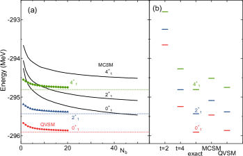
Figure 1: (a) Energy expectation values $E_{N_{b}}$ of the $0^{+}_{1}$ (red), $2^{+}_{1}$ (blue), $4^{+}_{1}$ (green) states of ¹³²Ba by the QVSM and the MCSM as a function of the number of the basis states $N_{b}$. The horizontal dotted lines show the exact shell-model energies. (b) The $0^{+}_{1}$, $2^{+}_{1}$, $4^{+}_{1}$ energies of ¹³²Ba obtained by the conventional Lanczos method with $t=2$ truncation, by that with $t=4$ truncation, by the exact calculation without truncation, by the MCSM with 50 basis states, and by the QVSM with 20 basis states are shown from left to right.

Figure 1(a) shows the QVSM energy as a function of the number of the basis states $N_{b}$, which is defined in Eq.(1). As $N_{b}$ increases the QVSM energy comes down and the energy converges rapidly and approaches the exact values shown in Fig. 1(b). Even at $N_{b}=1$, the QVSM energy is closer to the exact one than those of $t$-particle $t$-hole truncations and that of the MCSM.

The solid black lines in Fig. 1(a) also show the MCSM energy expectation values as a function of the number of the basis states, $N_{b}$. The MCSM wave function mcsm_ptep is defined as a linear combination of the angular-momentum and parity projected deformed Slater determinants as

$$|\Psi_{N_{b}}\rangle = \sum_{n=1}^{N_{b}}\sum_{K=-J}^{J}f^{(N_{b})}_{nK}P^{J\pi}_{MK}|D_{n}^{(\pi)}\rangle\otimes|D_{n}^{(\nu)}\rangle$$ (3)

where $|D_{n}^{(\pi)}\rangle$ and $|D_{n}^{(\nu)}\rangle$ are the deformed Slater determinants for protons and neutrons, respectively. The number projection is not necessary since a Slater determinant is an eigenstate of the number operator. The Slater determinant $|D_{n}\rangle$ is parametrized by the complex matrix $D_{n}$, which is determined to minimize the energy eigenvalue in the same way as the QVSM. Since Slater determinants cannot describe pairing correlations efficiently, the MCSM energy converges rather slowly in comparison with the QVSM.

For comparison, Figure 1 (b) shows the energies obtained by the QVSM, the MCSM, and the conventional Lanczos diagonalization method in truncated spaces. The conventional Lanczos method was performed with the truncated space restricting up to $t$-particle $t$-hole excitations across the $Z=N=64$ shell gap from the filling configuration. The truncation scheme is taken as $t=2$ ($2.3\times 10^{8}$ $M$-scheme dimension), $t=4$ ($3.4\times 10^{9}$ $M$-scheme dimension), and the full space without truncation for the exact energy. The $t=2$ ($t=4$) energy is 2.3 MeV (0.7 MeV) higher than the exact one. The rightmost part of Fig. 1 (b) shows the results of the MCSM with $N_{b}=50$ and the QVSM with $N_{b}=20$. The MCSM result overcomes the truncated results, but it is still 440 keV higher than the exact one and the MCSM underestimates the excitation energies 100 keV. The QVSM agrees with the exact one quite well within 50 keV. This small gap between the QVSM and exact ones can be filled by the energy-variance extrapolation method, which will be discussed in the next section.

While the QVSM converges as a function of $N_{b}$ apparently better than the MCSM, the computational cost of the QVSM with the same $N_{b}$ is heavier than that of the MCSM because of the necessity of the number projection. In practice, the total computational of the QVSM whose result is shown in Fig. 1 is about 10 times heavier than that of the MCSM. Even considering such difference, the QVSM is more efficient than the MCSM in the ¹³²Ba case since the QVSM energy with $N_{b}=1$ is already lower than the MCSM energy with $N_{b}=50$.

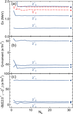
Figure 2: (a) Excitation energies of the $0^{+}_{2}$ and $0^{+}_{3}$ states (red dashed lines), and $2^{+}_{1}$, $2^{+}_{2}$, and $2^{+}_{3}$ states (blue solid lines) of ¹³²Ba against the number of the basis states $N_{b}$. (b) Quadrupole moments of the $2^{+}_{1}$, $2^{+}_{2}$, and $2^{+}_{3}$ states. (c) Square root of the B(E2) transition probabilities from the ground state to the $2^{+}_{1}$, $2^{+}_{2}$, and $2^{+}_{3}$ states. The triangles at the rightmost side denote the exact values.

For proving the feasibility of the QVSM to treat the nonyrast states and other physical quantities, we performed the variational calculations to obtain the lowest three $0^{+}$ and $2^{+}$ states of ¹³²Ba. We performed the variational calculations so that the summation of the lowest three energy expectation values is minimized. Figure 2 (a) shows the excitation energies of the $0^{+}_{2}$, $0^{+}_{3}$, $2^{+}_{1}$, $2^{+}_{2}$, and $2^{+}_{3}$ states as a function of the number of the basis states $N_{b}$. The extrapolation procedure is not required since these excitation energies converge quite rapidly at $N_{b}\simeq 10$ and agree with the exact values. Figures 2 (b) and (c) show the quadrupole moments and the square root of the B(E2) transition probabilities with the effective charges $(e_{p},e_{n})=(1.5,0.5)e$. These observables also show good convergence patterns and converge at $N_{b}\simeq 10$. Note that although $B(E2;0^{+}_{1}\rightarrow 2^{+}_{2})$ and $B(E2;0^{+}_{1}\rightarrow 2^{+}_{3})$ are quite small in comparison with the large $B(E2;0^{+}_{1}\rightarrow 2^{+}_{1})$ value, these three $B(E2)$ values converge rapidly at the same pace.

III Energy variance extrapolation

The variational calculation discussed in the previous section gives us only the variational upper limit to the exact shell-model energy. In order to estimate the exact energy more precisely, we here introduce the extrapolation method employing the energy variance. The energy-variance extrapolation was proposed in condensed matter physics sorella , and was introduced to the nuclear shell-model calculations in Ref. mizusaki_imada_extrap . Since then it was applied to various schemes mcsm_extrap ; itsm_extrap ; puddu_variance ; extrap_ncsm ; vmcsm .

The energy variance of the variational wave functions is defined as

$$\langle\Delta H^{2}\rangle_{N_{b}} = \langle\Psi_{N_{b}}|H^{2}|\Psi_{N_{b}}\rangle-\langle\Psi_{N_{b}}|H|\Psi_{N_{b}}\rangle^{2}.$$ (4)

A formula to compute the energy variance in the quasi-particle vacua is shown in Appendix A.3. By utilizing the fact that the energy variance is zero if $|\Psi_{N_{b}}\rangle$ is the exact shell-model eigenstate, the variance expectation value is not only an indicator for the approximation, but also can be used for the estimation of the exact energy eigenvalue by extrapolation. As $N_{b}$ increases, the QVSM wave function approaches the exact one and the corresponding variance approaches zero. In the extrapolation scheme, we plot the energy $E_{N_{b}}$ against the variance $\langle\Delta H^{2}\rangle_{N_{b}}$, which is called a variance-energy plot hereafter. On the plot, as $N_{b}$ increases the point is expected to approach the $y$ axis, namely $\langle\Delta H^{2}\rangle_{N_{b}}=0$, gradually. The extrapolated energy is the $y$ intercept of the curve fitted for these points.

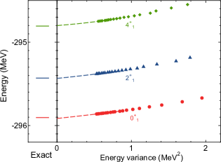
Figure 3: Variance-energy plot of ¹³²Ba. The red circles, blue triangles, and green diamonds denote the energy expectation values against the energy variance of the $0^{+}_{1}$, $2^{+}_{1}$, and $4^{+}_{1}$ states, respectively, obtained by the QVSM. The dashed curves are drawn to be fitted for the last 12 points of the QVSM results with a 2nd-order polynomial. and their $y$-intercepts are the extrapolated values. The left panel shows the exact shell-model energies.

Figure 3 shows the variance-energy plot of the QVSM wave functions of ¹³²Ba, which are the same as the case in Fig. 1. The last 12 points are used for the 2nd-order polynomial fit. The extrapolated values, which are the $y$ intercepts of the fitted lines, and the exact shell-model energies agree with each other quite well within a 10-keV difference.

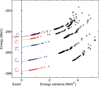
Figure 4: Variance-energy plot of ¹³²Ba. The red circles (blue triangles) denote the lowest three $0^{+}$ ($2^{+}$) states obtained by the QVSM. The black open circles (triangles) denote the energies and energy variances of the $0^{+}$ ($2^{+}$) states of the MCSM. The dashed curves are drawn to be fitted for the last 20 points of the QVSM results with a 2nd-order polynomial. and their $y$-intercepts are the extrapolated values. The left panel shows the exact shell-model energies.

Figure 4 shows variance-energy plots of the QVSM and the MCSM, whose wave functions are the same as the case of Fig. 2. While the left panel shows the exact shell-model energies the $y$-intercepts of the fitted curves are the extrapolated values of the QVSM results. The extrapolated energies and the exact shell-model energies obtained by the conventional Lanczos method agree quite well within a 20-keV difference.

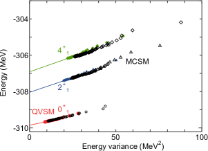
Figure 5: Variance-energy plot of ⁶⁸Ni with the A3DA interaction ytsunoda_ni . The red filled circles, blue filled triangles, and green filled diamonds are the QVSM results of the $0^{+}_{1}$, $2^{+}_{1}$, and $4^{+}_{1}$ states, respectively. The QVSM is obtained with $N_{b}=30$. The black symbols are the corresponding MCSM results with 120 basis states. The solid lines denote the fitted curves by a 1st-order polynomial for the last 13 QVSM points.

One of the major achievements of the MCSM is to reveal the exotic structure of neutron-rich nuclei around ⁶⁸Ni ytsunoda_ni . For further comparison of the QVSM and the MCSM, we show the variance-energy plot of the ⁶⁸Ni with the A3DA interaction ytsunoda_ni and the model space consisting of the $pf$ shell, $0g_{9/2}$, and $1d_{5/2}$ orbits in Fig. 5. The $M$-scheme dimension of this system is $5.2\times 10^{15}$, which is beyond the current feasibility of the conventional Lanczos method even now. The points of the MCSM and the points of the QVSM show a similar tendency. Although the QVSM with the 30 basis states provides us with the lower variational energy than that of the MCSM with the 120 basis states, the MCSM is advantageous in terms of the computation time since the number projection is not needed for the MCSM. According to our numerical experiments, the MCSM is more efficient for lighter nuclei such as $pf$-shell nuclei, while the QVSM is expected to be more efficient and to converge faster in medium-heavy mass region beyond the $N=Z=50$ gap such as ¹³²Ba. The feasibility and application of the QVSM to ¹⁵⁰Nd and the evaluation of its $0\nu\beta\beta$-decay NME will be discussed in the next section.

IV Neutrinoless double beta decay matrix elements

Here we focus on the convergence property of a NME of $0\nu\beta\beta$ decay in the QVSM and the MCSM. The $0\nu\beta\beta$-decay NME with the closure approximation is obtained as

$$M^{0\nu}=\langle 0^{+}_{f}|\hat{O}|0^{+}_{i}\rangle=M^{0\nu}_{GT}-\frac{g_{V}^{2}}{g_{A}^{2}}M^{0\nu}_{F}+M^{0\nu}_{T}$$ (5)

where $\hat{O}$ is the operator to annihilate two neutrons and create two protons with neutrino potential. $M^{0\nu}_{GT}$, $M^{0\nu}_{F}$ $M^{0\nu}_{T}$ denote the Gamow-Teller type, Fermi type, tensor type terms classified according to spin structure of the operator, respectively engel_menendez_bb_review . $|0^{+}_{i}\rangle$ and $|0^{+}_{f}\rangle$ are the ground states of the parent and daughter nuclei. $g_{V}$ and $g_{A}$ are vector and axial-vector coupling constants and are taken as 1.0 and 1.27, respectively. In the present work, a factor of short range correlation for the NME is omitted for simplicity and the average energy of the closure approximation is taken from the empirical formula $E_{\textrm{av}}=1.12\sqrt{A}$ MeV haxton .

As a benchmark test, we perform the shell-model calculation of ⁷⁶Ge and ⁷⁶Se with JUN45 interaction jun45 with the model space consisting of the $0f_{5/2}$, $1p_{3/2}$, $1p_{1/2}$, and $0g_{9/2}$ orbits both for protons and neutrons and evaluate the $0\nu\beta\beta$-decay NME. Since the $M$-scheme dimension of ⁷⁶Se is $6.8\times 10^{8}$, the exact shell-model value is obtained by the conventional Lanczos method more easily than the case of ¹³²Ba.

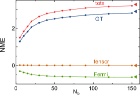
Figure 6: $0\nu\beta\beta$-decay NME of ⁷⁶Ge obtained by the MCSM. These values are shown as a function against the number of the basis states $N_{b}$. The red, blue, green, orange lines with the solid circles denote the total, GT-type, Fermi-type, and tensor-type NMEs, respectively. The circles show the MCSM values with $N_{b}=5,10,15,20,30,40,50,60,70,90,120,$ and 150. The exact shell-model values are shown as the triangles at the rightmost.

Figure 6 shows the NME obtained by the MCSM against the number of the basis states $N_{b}$. The MCSM calculation is performed up to $N_{b}=150$. The NME of the MCSM shows quite slow convergence as a function of the number of the basis states and the extrapolation using the MCSM results to the exact solution seems to be difficult. Since a $0\nu\beta\beta$-decay NME is sensitive to pairing correlations caurier2008 ; menendez2009 ; dgt_bb , the QVSM scheme is expected to be advantageous over the MCSM. To evaluate the NME using the linear combination of quasi-particle vacua as a wave function was also discussed in the context of the generator coordinate method yao_gcm_srg_1 ; yao_gcm_srg_2 ; yao_gcm_srg_3 ; gcm_bb ; rodriguez_150Nd .

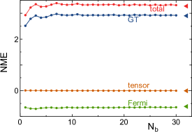
Figure 7: $0\nu\beta\beta$-decay NME of the ⁷⁶Ge against $N_{b}$ obtained by the QVSM. The exact values are shown as the triangles at the rightmost.

Figure 7 shows the NMEs obtained by the QVSM. The NMEs of the QVSM converge quite fast and agree well with the exact shell-model values. While the total NME of the MCSM is too small at $N_{b}=1$, the NMEs of the QVSM are close to the exact one even at $N_{b}=1$. It implies that the efficient treatment of the pairing correlation is essential for the estimation of the $0\nu\beta\beta$ NMEs.

We evaluate the NMEs of the $0\nu\beta\beta$ decay of ¹⁵⁰Nd by the QVSM and the MCSM. We adopt the Kuo-Herling interaction khhe with the model space consisting of $0g_{7/2}$, $1d_{5/2}$, $1d_{3/2}$, $2s_{1/2}$, and $0h_{11/2}$ orbits for protons and $0h_{9/2}$, $1f_{7/2}$, $1f_{5/2}$, $2p_{3/2}$, $2p_{1/2}$, and $0i_{13/2}$ orbits for neutrons with the ¹³²Sn inert core. The $M$-scheme dimension of ¹⁵⁰Nd is $2.2\times 10^{14}$, far beyond the current limitation of the conventional Lanczos method. ¹⁵⁰Nd is one of nuclei whose NME has not been evaluated by reliable shell-model calculations among major double-beta-decay nuclei used for $0\nu\beta\beta$-decay search experiments engel_menendez_bb_review .

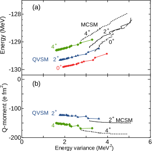
Figure 8: Energy expectation values (a) and spectroscopic quadrupole moments (b) of the yrast states of ¹⁵⁰Nd obtained by the QVSM with $N_{b}=20$ and the MCSM with $N_{b}=100$ against the energy variance. The red circles, blue triangles, and green diamonds denote the QVSM results of the $0^{+}$, $2^{+}$ and $4^{+}$ states, respectively. The dashed, solid, and dotted lines are the MCSM results of the $0^{+}$, $2^{+}$ and $4^{+}$ states, respectively. The effective charges are taken as $(e_{p},e_{n})=(1.58,0.85)e$.

Figures 8 (a) and 9 (a) show the variance-energy plots of the $0^{+}$, $2^{+}$ and $4^{+}$ states of ¹⁵⁰Nd and ¹⁵⁰Sm, respectively. These are obtained by the QVSM with $N_{b}=20$ and the MCSM with $N_{b}=100$. The QVSM energies are about 1 MeV lower, and therefore better, than those of the MCSM, While the MCSM results do not reach the convergence even at $N_{b}=100$, the QVSM results show good convergence. The $0^{+}$, $2^{+}$, and $4^{+}$ energies of the QVSM converge in a similar way, which means the excitation energies converge stably. Figures 8 (b) and 9 (b) show the spectroscopic quadrupole moments of the QVSM and the MCSM results against the energy variance. The QVSM results show stable convergence, while the MCSM overestimates the deformation.

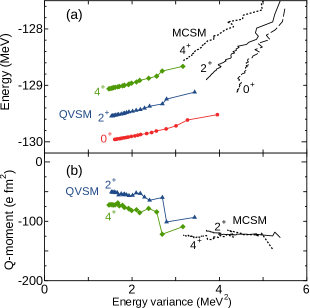
Figure 9: Energy expectation values (a) and spectroscopic quadrupole moments (b) of the yrast states of ¹⁵⁰Sm obtained by the QVSM and the MCSM against the energy variance. See caption of Fig. 8 for details.

Figure 10: Excitation energies of the $2^{+}$ and $4^{+}$ states of (a) ¹⁵⁰Nd and (b) ¹⁵⁰Sm as a function of the QVSM basis states.

Figure 10 shows the excitation energies of ¹⁵⁰Nd and its daughter nucleus, ¹⁵⁰Sm, obtained by the QVSM. The energies of the QVSM converge well as a function of $N_{b}$. The QVSM result of the $2^{+}$ energy of the ¹⁵⁰Nd is 240 keV which is larger than the experimental value, 130 keV. Besides, the quadrupole moment by the QVSM is $-1.2$ eb, which shows smaller deformation than the experimental value, $-2.0(5)$ eb. It may indicate that the larger model space is required to describe the large quadrupole deformation of ¹⁵⁰Nd, which is also indicated by Refs. Yao_PRC91 ; otsuka_sm .

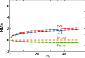
Figure 11: $0\nu\beta\beta$-decay NME of the ¹⁵⁰Nd obtained by the MCSM against the number of the basis states $N_{b}$. The red, blue, green, orange lines with the solid circles denote the total, GT-type, Fermi-type, and tensor-type NMEs, respectively.

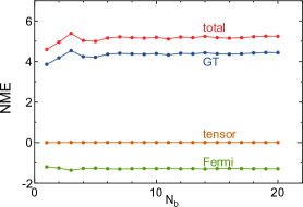
Figure 12: $0\nu\beta\beta$-decay NME of the ¹⁵⁰Nd obtained by the QVSM against the number of the basis states $N_{b}$. The red, blue, green, orange lines with the solid circles denote the total, GT-type, Fermi-type, and tensor-type NMEs, respectively.

Figure 11 shows the NME of the MCSM against the number of the basis states. The convergence of the NME is quite slow and it is difficult to estimate the converged value. Figure 12 shows the NME values by the QVSM. The NMEs converge quite rapidly in contrast to the MCSM case in Fig. 11, and these values do not change where $N_{b}$ is beyond 10 owing to the efficient description by the quasi-particle-vacuum basis states. Although this NME value is not conclusive since the present study overestimates the excitation energies, it is worth comparing it with previous works briefly. The total NME of the current work is 5.2, which is about twice larger than other proceeding results of the quasi-particle random phase approximation and several other approaches QRPA_CH . The NME values given by the latest generator-coordinate method based on the relativistic energy density functional are 5.6 Yao_PRC91 and 5.2 YaoEngel_PRC94 , which are close to the present result. It was suggested that the large difference between the deformations of the initial and final states would suppress the NME song_RMF_150Nd ; rodriguez_150Nd ; FangFaessler2010 . Further investigation by extending the model space is ongoing to evaluate the effect of the large quadrupole deformation and its differences between the initial and final states appropriately.

V Summary

We have developed a variational method after the superposition of the fully projected quasi-particle vacua, named the quasi-particle vacua shell model (QVSM), which is an extension of the MCSM. We apply the energy-variance extrapolation method to the QVSM and demonstrated that it works quite well to estimate the shell-model energies of ¹³²Ba with the SN100PN interaction. The excitation energies and other observables such as the quadrupole moment and $B(E2)$ transition probabilities by the QVSM converge quite rapidly as a function of the number of the basis states. Since the QVSM wave function is expected to include many-body correlations such as pairing correlations efficiently, it works well in nuclei heavier than Sn isotopes, while the MCSM is efficient enough in lighter-mass region such as ⁶⁸Ni in terms of computational resources.

We have demonstrated that the NME values of the QVSM against $N_{b}$ show fast convergence. The feasibility of the QVSM to evaluate the $0\nu\beta\beta$-decay NME of ¹⁵⁰Nd is validated. Since the shell-model result of the Kuo-Herling interaction overestimates the experimental $2^{+}$ and $4^{+}$ excitation energies of ¹⁵⁰Nd and ¹⁵⁰Sm, further investigation is anticipated to conclude the NME values by shell-model calculations. We also plan to evaluate the NMEs of double-beta-decay nuclei in medium-heavy mass region such as ¹³⁶Xe kamland and ¹⁰⁰Mo, which will be used for the next-generation $0\nu\beta\beta$-decay search experiment cupid .

This proof-of-the-principle study opens a way to investigate the medium-heavy nuclei with configuration mixing utilizing nuclear shell-model calculations. The application of the present scheme to odd nuclei would be rather straightforward and is under progress.

Appendix A Matrix elements between different quasi-particle vacua

In this appendix, we briefly show some equations which are required for the QVSM scheme. Since the QVSM wave function defined in Eq.(1) is written as a linear combination of the projected quasi-particle vacua, we need the equations to compute the overlap, the Hamiltonian matrix elements, and the energy gradient between two different quasi-particle vacua. In addition, we firstly derive the equation of the matrix elements of the Hamiltonian squared for the energy-variance extrapolation technique.

The overlap between two different quasi-particle vacua is computed by the Neergard-Wust method neergardwust in the present work for efficient computations, while more elegant formula employing the Pfaffian was suggested robledo_pfaffian . Some overlap formulae for odd-mass case were proposed AvezBender ; bertsch_robledo ; oimizusaki_odd .

The shell-model Hamiltonian is defined as

$$H=\sum_{ij}t_{ij}c^{\dagger}_{i}c_{j}+\frac{1}{4}\sum_{ijkl}v_{ijkl}c^{\dagger}_{i}c^{\dagger}_{j}c_{l}c_{k}$$ (6)

where $t$ and $v$ are the coefficients of the one-body and two-body interactions, respectively. $v$ is Hermitian ($v_{ijkl}=v_{klij}$) and anti-symmetrized ($v_{ijkl}=-v_{jikl}=-v_{ijlk}=v_{jilk}$).

A.1 Hamiltonian matrix elements

.

We show equations for the energy expectation values of the QVSM wave function. The QVSM wave function is a linear combination of the angular-momentum, parity, number projected quasi-particle vacua. In numerical calculations, the angular-momentum projector is calculated as the summation of the discretized Euler angles $\Omega=(\alpha,\beta,\gamma)$, and the parity projection is performed utilizing the parity-conversion operator $\Pi$ mcsm_ptep :

$$P^{J\pi}_{MK} = \frac{1+\pi\Pi}{2}\frac{2J+1}{8\pi^{2}}\int d\Omega\ D^{J*}_{MK}(\Omega)e^{i\alpha J_{z}}e^{i\beta J_{y}}e^{i\gamma J_{z}}$$ (7)

$$\simeq \sum_{a}W_{a}^{JMK\pi}R_{a}$$

with

$$R_{a} = e^{i\alpha_{a}J_{z}}e^{i\beta_{a}J_{y}}e^{i\gamma_{a}J_{z}}\Pi^{(\delta_{a})},$$ (8)

$$W_{a}^{JMK\pi} = \frac{2J+1}{8\pi^{2}}D^{J*}_{MK}(\alpha_{a},\beta_{a},\gamma_{a})\pi^{(\delta_{a})}w_{a},$$

$\pi^{(1)}=\frac{1}{2},\pi^{(2)}=\frac{\pi}{2},\Pi^{(1)}=1,\Pi^{(2)}=\Pi$, and $a=(\alpha_{a},\beta_{a},\gamma_{a},\delta_{a})$ mcsm_ptep . $a$ and $w_{a}$ are a set of discretized mesh points and its corresponding weight for the summation, and are determined by the Gaussian quadrature num_recipe . The proton number projector is also computed as

$$P^{Z}=\frac{1}{2\pi}\int_{0}^{2\pi}e^{i\phi(N^{(\pi)}-Z)}d\phi\simeq\sum_{b=1}^{L}W_{b}^{(Z)}R^{(Z)}_{b}$$ (9)

where $N^{(\pi)}$ denotes the proton number operator and $R^{(Z)}_{b}=e^{2\pi iN^{(\pi)}b/L}$, $W_{b}^{(Z)}=\frac{1}{L}e^{-2\pi iZb/L}$. The neutron number projector is defined in the same way as the proton case.

Thus, the coefficient of the QVSM wave function $f^{(N_{b})}_{iK}$ in Eq.(1) and its energy expectation value are obtained by solving the generalized eigenvalue problem, or the Hill-Wheeler-Griffin equation hillwheeler ,

$$\sum_{j=1}^{N_{b}}\sum_{K^{\prime}=-J}^{J}\left(H_{iK,jK^{\prime}}-E_{N_{b}}N_{iK,jK^{\prime}}\right)f^{(N_{b})}_{jK^{\prime}}=0$$ (10)

with

$$H_{iK,jK^{\prime}} = \sum_{a}W_{a}^{JKK^{\prime}\pi}\langle\phi_{i}^{(\pi)}|\otimes\langle\phi_{i}^{(\nu)}|HR_{a}$$

$$\sum_{b}W_{b}^{(Z)}R^{(Z)}_{b}|\phi_{j}^{(\pi)}\rangle\otimes\sum_{c}W_{c}^{(N)}R^{(N)}_{c}|\phi_{j}^{(\nu)}\rangle.$$

$$N_{iK,jK^{\prime}} = \sum_{a}W_{a}^{JKK^{\prime}\pi}\langle\phi_{i}^{(\pi)}|\otimes\langle\phi_{i}^{(\nu)}|R_{a}$$

$$\sum_{b}W_{b}^{(Z)}R^{(Z)}_{b}|\phi_{j}^{(\pi)}\rangle\otimes\sum_{c}W_{c}^{(N)}R^{(N)}_{c}|\phi_{j}^{(\nu)}\rangle.$$

Note that $f_{iK}^{(N_{b})}$ is determined so that the resultant wave function is normalized. The number of the mesh points of the angular-momentum, parity projector typically reaches 60,000 and the matrix element for each $a$ can be computed in parallel. This feature is suitable for massively parallel computations. Since the computational cost for such variation after projection is quite heavy, we utilized state-of-the-art supercomputers in Japan such as Fugaku and Oakforest-PACS. The developed code is equipped with the code-tuning technique suggested in Ref. mcsm_tuning .

Hereafter, we consider only protons for simplicity. The derivation of its extension to the proton-neutron system is lengthy but straightforward. Since the rotated quasi-particle vacuum $R|\phi\rangle$ can be expressed as another quasi-particle vacuum by using the Baker-Campbell-Hausdorff formula, we need to compute the matrix element of the Hamiltonian between two different quasi-particle vacua. Note that the $f^{(N_{b})}_{iK}$ is obtained by solving Eq.(10) every time its basis state is changed.

The Hamiltonian matrix element between the different quasi-particle vacua, $|\phi\rangle$ and $|\phi^{\prime}\rangle$, is calculated using the generalized Wick theorem ringschuck as

$$\langle\phi|H|\phi^{\prime}\rangle = \langle\phi|\phi^{\prime}\rangle\textrm{Tr}\left(t\rho+\frac{1}{2}\Gamma\rho-\frac{1}{2}\kappa^{\prime}\Delta\right)$$ (13)

where the density matrix $\rho$ and the pairing tensor $\kappa$ are obtained as

$$\rho_{ij} = \frac{\langle\phi|c^{\dagger}_{j}c_{i}|\phi^{\prime}\rangle}{\langle\phi|\phi^{\prime}\rangle}=-Z^{\prime}(1-Z^{*}Z^{\prime})^{-1}Z^{*}$$ (14)

$$\kappa_{ij} = \frac{\langle\phi|c_{j}c_{i}|\phi^{\prime}\rangle}{\langle\phi|\phi^{\prime}\rangle}=Z^{\prime}(1-Z^{*}Z^{\prime})^{-1}$$ (15)

$$\kappa^{\prime}_{ij} = \frac{\langle\phi|c^{\dagger}_{i}c^{\dagger}_{j}|\phi^{\prime}\rangle}{\langle\phi|\phi^{\prime}\rangle}=(1-Z^{*}Z^{\prime})^{-1}Z^{*}$$ (16)

$$Z = (VU^{-1})^{*}$$

$$Z^{\prime} = (V^{\prime}U^{\prime-1})^{*}$$ (17)

$$\Gamma_{ik} = \sum_{jl}v_{ijkl}\rho_{lj}$$

$$\Delta_{ij} = \frac{1}{2}\sum_{kl}v_{ijkl}\kappa_{kl}.$$ (18)

A.2 Energy gradient

In the QVSM scheme, we apply the conjugate gradient method to minimize the projected energy expectation value. The basis state $|\phi_{n}\rangle$ is determined sequentially so that the energy expectation value $E_{N_{b}=n}$ is minimized. Let us consider the situation that $N_{b}-1$ basis states have already been fixed and the variational calculation is performed with the variational parameters of the $N_{b}$-th basis state, $Z^{(N_{b})}$, by the conjugate gradient method, which requires the gradient of the projected energy of the superposed quasi-particle vacua. The energy gradient is obtained as

$$\frac{\partial E_{N_{b}}}{\partial Z^{(N_{b})*}} = \sum_{n,KK^{\prime}}(f^{(N_{b})}_{N_{b}K^{\prime}})^{*}f^{(N_{b})}_{nK}\frac{\partial\langle\phi_{N_{b}}|}{\partial Z^{(N_{b})*}}$$ (19)

$$(H-E_{N_{b}})P^{J\pi}_{K^{\prime}K}P^{Z}|\phi_{n}\rangle,$$

where the matrix element of the gradient is obtained as

$$\frac{\partial\langle\phi|}{\partial Z^{*}}(H-E_{N_{b}})|\phi^{\prime}\rangle$$ (20)

$$= \langle\phi|\phi^{\prime}\rangle(U_{D}^{\dagger}(t+\Gamma)V_{D}^{*}-V_{D}^{\dagger}(t+\Gamma)^{T}U_{D}^{*}$$

$$+U_{D}^{\dagger}\Delta U_{D}^{*}-V_{D}^{\dagger}\Delta^{\prime}V_{D}^{*})$$

$$-Z_{D}\langle\phi^{\prime}|(H-E_{N_{b}})|\phi\rangle$$

with

$$Z_{D} = ((V^{T}U^{\prime}+U^{T}V^{\prime})(U^{\dagger}U^{\prime}+V^{\dagger}V^{\prime})^{-1})^{*}$$

$$U_{D} = U+V^{*}Z_{D}^{*}$$

$$V_{D} = V+U^{*}Z_{D}^{*}.$$

$$\Delta^{\prime}_{kl} = \frac{1}{2}\sum_{ij}\kappa^{\prime}_{ij}v_{ijkl}.$$ (21)

A.3 Energy variance

Since the energy variance is the expectation value of the four-body operator, the computation of the energy variance is time-consuming and its efficient computation is essential for practical applications. By utilizing the separability of $H^{2}$ in a similar way to the case of Slater determinants in Ref. mcsm_extrap , a formula to compute the matrix element of the Hamiltonian squared between two quasi-particle vacua is given as

$$\langle\phi|H^{2}|\phi^{\prime}\rangle$$ (22)

$$= \langle\phi|\phi^{\prime}\rangle\Big{(}\frac{1}{4}\sum_{ijkl}(\rho^{\prime}v\rho)_{ijkl}(\rho v\rho^{\prime})_{klij}$$

$$+\frac{1}{4}\sum_{ijkl}(\kappa^{\prime}v\kappa)_{ijkl}(\kappa^{\prime}v\kappa)_{jilk}-\sum_{ijkl}(\rho^{\prime}v\rho)_{ijkl}(\kappa^{\prime}v\kappa)_{jkli}$$

$$+\frac{1}{2}\textrm{Tr}\big{(}(\rho\Gamma_{t}-\kappa\Delta^{\prime})(\rho^{\prime}\Gamma_{t}+\kappa\Delta^{\prime})$$

$$\ \ \ \ \ \ +(\Gamma_{t}\rho-\Delta\kappa^{\prime})(\Gamma_{t}\rho^{\prime}+\Delta\kappa^{\prime})$$

$$\ \ \ \ \ \ -(\kappa\Gamma_{t}^{T}-\rho\Delta)(\kappa^{\prime}\Gamma_{t}-\rho^{T}\Delta^{\prime})$$

$$\ \ \ \ \ \ -(\kappa\Gamma_{t}^{T}+\rho^{\prime}\Delta)(\kappa^{\prime}\Gamma_{t}+\rho^{\prime T}\Delta^{\prime})\big{)}$$

$$+\big{(}\textrm{Tr}(t\rho+\frac{1}{2}\Gamma\rho-\frac{1}{2}\kappa^{\prime}\Delta)\big{)}^{2}\Big{)}$$

with

$$\rho^{\prime}_{ij} = \delta_{ij}-\rho_{ij}$$

$$(\Gamma_{t})_{ij} = \Gamma_{ij}+t_{ij}$$

$$(\rho^{\prime}v\rho)_{ijkl} = \sum_{a,c}\rho^{\prime}_{ia}v_{ajcl}\rho_{ck}$$

$$(\rho v\rho^{\prime})_{ijkl} = \sum_{b,d}\rho_{jb}v_{ibkd}\rho^{\prime}_{dl}$$

$$(\kappa^{\prime}v\kappa)_{ijkl} = \sum_{ac}\kappa^{\prime}_{ia}v_{ajcl}\kappa_{ck}.$$ (23)

The angular-momentum, parity, and number projections can be applied in the same way as described in Appendix A.1. The most time-consuming part in practical calculations is to compute $(\rho^{\prime}v\rho)_{ijkl}$ as

$$(\rho^{\prime}v\rho)_{ijkl}=\sum_{a}\rho^{\prime}_{ia}\left(\sum_{c}v_{ajcl}\rho_{ck}\right).$$ (24)

This is computed by the summations of the fivefold loops, which cost far smaller than the case of a general four-body operator demanding eightfold loops.

References

- (1) E. Caurier, G. Martinez-Pinedo, F. Nowacki, A. Poves, and A. P. Zuker, Rev. Mod. Phys. 77, 427 (2005).
- (2) T. Otsuka, A. Gade, O. Sorlin, T. Suzuki, and Y. Utsuno Rev. Mod. Phys. 92, 015002 (2020).
- (3) J. P. Vary, P. Maris, E. Ng, C. Yang, and M. Sosonkina, J. Phys.: Conf. Ser. 180 012083 (2009).
- (4) C. W. Johnson, W. E. Ormand, and P. G. Krastev, Comp. Phys. Comm. 184, 2761 (2013).
- (5) N. Shimizu, T. Mizusaki, Y. Utsuno, and Y. Tsunoda, Comp. Phys. Comm. 244, 372 (2019).
- (6) K. Hara and Y. Sun, Int. J. Mod. Phys. E 4, 637 (1995); Y. Sun, K. Hara, J. A. Sheikh, J G. Hirsch, V. Velazquez, and M. Guidry, Phys. Rev. C 61, 064323 (2000).
- (7) Y. M. Zhao and A. Arima, Phys. Rep. 545, 1 (2014).
- (8) K. Higashiyama and N. Yoshinaga, Phys. Rev. C 83, 034321 (2011).
- (9) T. Otsuka, M. Honma, T. Mizusaki, N. Shimizu, and Y. Utsuno, Prog. Part. Nucl. Phys. 47, 319 (2001).
- (10) N. Shimizu, T. Abe, M. Honma, T. Otsuka, T. Togashi, Y. Tsunoda, Y. Utsuno, and T. Yoshida, Phys. Scr. 92, 063001 (2017); N. Shimizu, T. Abe, Y. Tsunoda, Y. Utsuno, T. Yoshida, T. Mizusaki, M. Honma, and T. Otsuka, Prog. Theor. Exp. Phys. 2012, 01A205 (2012)
- (11) K. W. Schmid, F. Grummer, and A. Faessler, Annal. Phys. 180, 1 (1987).
- (12) K. W. Schmid, Prog. Part. Nucl. Phys. 46, 145 (2001).
- (13) G. Puddu, J. Phys. G: Nucl. Phys. 46, 115103 (2019).
- (14) D. Bianco, N. Lo Iudice, F. Andreozzi, A. Porrino, and F. Knapp, Phys. Rev. C 88, 024303 (2013).
- (15) L. F. Jiao, Z. H. Sun, Z. X. Xu, F. R. Xu and C. Qi, Phys. Rev. C 90, 024306 (2014).
- (16) O. Legeza, L. Veis, A. Poves, and J. Dukelsky Phys. Rev. C 92, 051303(R) (2015).
- (17) C. Stumpf, J. Braun, and R. Roth, Phys. Rev. C 93, 021301(R) (2016).
- (18) B. Bally, A. S. Fernandez, T. R. Rodriguez, Phys. Rev. C 100, 044308 (2019).
- (19) J. M. Yao, J. Engel, L. J. Wang, C. F. Jiao, and H. Hergert, Phys. Rev. C 98, 054311 (2018).
- (20) J. M. Yao, A. Bally, J. Engel, R. Wirth, T. R. Rodriguez, and H. Hergert, Phys. Rev. Lett. 124, 232501 (2020).
- (21) J. M. Yao, A. Bally, R. Wirth, T. Miyagi, C. G. Payne, S. R. Stroberg, H. Hergert, and J. D. Holt, arXiv:2010.08609
- (22) S. E. Koonin, D. J. Dean, and K. Langanke, Phys. Rep. 278, 1 (1997).
- (23) Y. Alhassid, G. F. Bertsch, D. J. Dean, and S. E. Koonin, Phys. Rev. Lett. 77, 1444 (1996).
- (24) J. Bonnard and O. Juillet, Phys. Rev. Lett. 111, 012502 (2013).
- (25) N. Shimizu, Y. Utsuno, T. Mizusaki, T. Otsuka, T. Abe, and M. Honma, Phys. Rev. C 82, 061305(R) (2010); N. Shimizu, Y. Utsuno, T. Mizusaki, M. Honma, Y. Tsunoda, and T. Otsuka, Phys. Rev. C 85, 054301 (2012).
- (26) T. Otsuka, M. Honma, and T. Mizusaki, Phys. Rev. Lett. 81, 1588 (1998).
- (27) Y. Tsunoda, T. Otsuka, N. Shimizu, M. Honma, and Y. Utsuno Phys. Rev. C 89, 031301(R) (2014).
- (28) Y. Utsuno, T. Otsuka, T. Mizusaki and M. Honma, Phys. Rev. C 60, 054315 (1999).
- (29) N. Tsunoda, T. Otsuka, N. Shimizu, M. H.-Jensen, K. Takayanagi, and T. Suzuki, Phys. Rev. C 95, 021304(R) (2017).
- (30) N. Tsunoda, T. Otsuka, K. Takayanagi, N. Shimizu, T. Suzuki, Y. Utsuno, S. Yoshida and H. Ueno, Nature 587, 66 (2020).
- (31) L. Liu, T. Otsuka, N. Shimizu, Y. Utsuno and R. Roth, Phys. Rev. C 86, 014302 (2012).
- (32) T. Abe, P. Maris, T. Otsuka, N. Shimizu, Y. Utsuno, and J. P. Vary, Phys. Rev. C 86, 054301 (2012).
- (33) T. Togashi, Y. Tsunoda, T. Otsuka, and N. Shimizu, Phys. Rev. Lett. 117, 172502 (2016).
- (34) T. Togashi, Y. Tsunoda, T. Otsuka, and N. Shimizu, Phys. Rev. Lett. 117, 172502 (2016).
- (35) T. Otsuka, Y. Tsunoda, T. Abe, N. Shimizu, and P. Van Duppen, Phys. Rev. Lett. 123, 222502 (2019).
- (36) A. Bohr, B. R. Mottelson, and D. Pines, Phys. Rev. 110, 936 (1958).
- (37) N. Shimizu, T. Otsuka, T. Mizusaki, and M. Honma, Phys. Rev. Lett. 86, 1171 (2001).
- (38) J. L. Egido and P. Ring, Nucl. Phys. A383 189 (1982).
- (39) F. T. Avignone III, S. R. Eliott, J. Engel, Rev. Mod. Phys. 80, 481 (2008).
- (40) J. Engel and J. Menendez, Rep. Prog. Phys. 80, 046301 (2017).
- (41) E. Caurier, F. Nowacki, A. Poves, and J. Retamosa, Phys. Rev. Lett. 77, 1954 (1996).
- (42) Y. Iwata, N. Shimizu, T. Otsuka, Y. Utsuno, J. Menendez, M. Honma and T. Abe, Phys. Rev. Lett. 116, 112502 (2016).
- (43) N. Shimizu, J. Menendez, and K. Yako, Phys. Rev. Lett. 120, 142502 (2018).
- (44) J. Menendez, A. Poves, E.Caurier, F.Nowacki, Nucl. Phys. A 818, 139 (2009).
- (45) L. Coraggio, A. Gargano, N. Itaco, R. Mancino, and F. Nowacki, Phys. Rev. C 101, 044315 (2020).
- (46) P. Ring and P. Schuck, “The Nuclear Many-Body Problem”, Springer (1980).
- (47) Numerical Recipes in Fortran 77, the Art of Scientific Computing, 1992 (Cambridge University Press, Cambridge, UK), 2nd ed.
- (48) A. Petrovici, K. W. Schmid, A. Fassler, J. M. Hamilton and A. V. Ramayya, Prog. Part. Nucl. Phys. 43, 485 (1999).
- (49) B. A. Brown, N. J. Stone, J. R. Stone, I. S. Towner, and M. Hjorth-Jensen, Phys. Rev. C 71, 044317 (2005).
- (50) S. Sorella, Phys. Rev. B 64, 024512 (2001).
- (51) T. Mizusaki and M. Imada, Phys. Rev. C 65, 064319 (2002); ibid. 67, 041301(R) (2003).
- (52) G. Puddu, J. Phys. G: Nucl. Part. Phys. 39, 085108 (2012).
- (53) H. Zhan, A. Nogga, B. R. Barrett, J. P. Vary, and P. Navratil, Phys. Rev. C 69, 034302 (2004).
- (54) N. Shimizu, and T. Mizusaki, Phys. Rev. C 98, 054309 (2018), T. Mizusaki and N. Shimizu, Phys. Rev. C 98, 054309 (2018).
- (55) W. C. Haxton and G.J. Stephenson Jr., Prog. Part. Nucl. Phys. 12, 409 (1984).
- (56) M. Honma, T. Otsuka, T. Mizusaki, and M. Hjorth-Jensen, Phys. Rev. C 80, 064323 (2009).
- (57) E. Caurier, J. Menendez, F. Nowacki, and P. Poves, Phys. Rev. Lett. 100, 052503 (2008)
- (58) T. R. Rodriguez and G. M.-Pinedo Phys. Rev. Lett. 105, 252503 (2010).
- (59) C. F. Jiao, J. Engel, and J. D. Holt, Phys. Rev. C 96, 054310 (2017).
- (60) T. T. S. Kuo and G. Herling, US Naval Research Laboratory Report No. 2258, 1971 (unpublished), Nucl. Phys. A 181, 113 (1972).
- (61) J. M. Yao, L. S. Song, K. Hagino, P. Ring, and J. Meng, Phys. Rev. C 91, 024316 (2015).
- (62) M. T. Mustonen and J. Angel, Phys. Rev. C 87, 064302 (2013).
- (63) J. M. Yao and J. Engel Phys. Rev. C 94, 014306 (2016).
- (64) L. S. Song, J. M. Yao, P. Ring, and J. Meng Phys. Rev. C 90, 054309 (2014).
- (65) D.-L. Fang, A. Faessler, V. Rodin, and F. Simkovic, Phys. Rev. C 82, 051301(R) (2010).
- (66) A. Gando et al., Phys. Rev. C 86, 021601(R) (2012).
- (67) E. Armengaud et al., Euro. Phys. J. C 80, 44 (2020).
- (68) K. Neergard and E. Wust, Nucl. Phys. A402 311 (1983).
- (69) L. M. Robledo, Phys. Rev. C 79, 021302(R) (2009).
- (70) B. Avez and M. Bender Phys. Rev. C 85, 034325 (2012).
- (71) G. F. Bertsch and L. M. Robledo Phys. Rev. Lett. 108, 042505 (2012).
- (72) M. Oi and T. Mizusaki, Phys. Lett. B 707, 305 (2012).
- (73) J. J. Griffin and J. A. Wheeler, Phys. Rev. 80, 367 (1966).
- (74) Y. Utsuno, N. Shimizu, T. Otsuka and T. Abe, Comput. Phys. Comm. 184, 102 (2013).