Efficient Hyperparameter Tuning with Dynamic Accuracy Derivative-Free Optimization

Abstract

Many machine learning solutions are framed as optimization problems which rely on good hyperparameters. Algorithms for tuning these hyperparameters usually assume access to exact solutions to the underlying learning problem, which is typically not practical. Here, we apply a recent dynamic accuracy derivative-free optimization method to hyperparameter tuning, which allows inexact evaluations of the learning problem while retaining convergence guarantees. We test the method on the problem of learning elastic net weights for a logistic classifier, and demonstrate its robustness and efficiency compared to a fixed accuracy approach. This demonstrates a promising approach for hyperparameter tuning, with both convergence guarantees and practical performance.

1 Introduction

Tuning model hyperparameters is a common problem encountered in machine learning for estimating regularization parameters, learning rates, and many other important quantities. In many cases, hyperparameter tuning can be viewed as a bilevel optimization problem for hyperparameters $\theta$:

$$\min_{\theta,w}F(\theta,w)\qquad\text{subject to}\qquad w\in\operatorname*{arg\,min}_{\widetilde{w}}\Phi(\widetilde{w},\theta),$$ (1)

where the lower-level objective $\Phi$ corresponds to a learning problem for weights $w$, and the upper-level objective $F$ typically measures a test error. Hyperparameter tuning often uses global optimization methods [Feurer and Hutter(2019)], but recent work has also considered local gradient-based [Luketina et al.(2016)Luketina, Berglund, Greff, and Raiko, Shaban et al.(2019)Shaban, Cheng, Hatch, and Boots] and derivative-free [Ghanbari and Scheinberg(2017), Lakhmiri et al.(2019)Lakhmiri, Le Digabel, and Tribes] methods. The lower-level problem is usually solved with iterative methods, so only inexact evaluations of feasible $w$ are available. As a result, few algorithms have convergence theory; exceptions include [Li et al.(2018)Li, Jamieson, DeSalvo, Rostamizadeh, and Talwalkar], [Shaban et al.(2019)Shaban, Cheng, Hatch, and Boots] under specific assumptions and [Ghanbari and Scheinberg(2017)] (in light of [Chen et al.(2018)Chen, Menickelly, and Scheinberg]). Bilevel learning is also used in inverse problems (e.g. [Arridge et al.(2019)Arridge, Maass, Öktem, and Schönlieb, Kunisch and Pock(2013), Ochs et al.(2015)Ochs, Ranftl, Brox, and Pock, Sherry et al.(2020)Sherry, Benning, los Reyes, Graves, Maierhofer, Williams, Schönlieb, and Ehrhardt]), although other approaches exist [Engl et al.(1996)Engl, Hanke, and Neubauer, Benning and Burger(2018), Hansen(1992)].

Recently in [Ehrhardt and Roberts(2020)], a model-based DFO method [Conn et al.(2009)Conn, Scheinberg, and Vicente, Audet and Hare(2017)] for bilevel learning (in an inverse problems context) was proposed, which has convergence guarantees while still allowing inexact lower-level minimizers (but with a dynamic accuracy controlled by the algorithm). Here, we apply this algorithm to bilevel optimization for hyperparameter tuning (1). Specifically, we apply the framework of [Ehrhardt and Roberts(2020)] to the case where the lower-level objective is nonsmooth (but strongly convex). Our approach has similarities to Hyperband [Li et al.(2018)Li, Jamieson, DeSalvo, Rostamizadeh, and Talwalkar], which considers an inexact Bayesian optimization method, whereas our approach is designed to exploit the bilevel structure to find a local minimum. We can achieve the dynamic accuracy requirements for the upper-level algorithm, but delegate full convergence theory to future work (noting that model-based DFO methods for nonsmooth problems exist; e.g. [Garmanjani et al.(2016)Garmanjani, Júdice, and Vicente, Grapiglia et al.(2016)Grapiglia, Yuan, and Yuan, Khan et al.(2018)Khan, Larson, and Wild]). We show results for tuning elastic net weights of a logistic classifier. Compared to fixed-accuracy variants of the same DFO method, our approach has strong computational performance and robustness, and avoids manually tuning the lower-level problem solution accuracy.

2 Lower-Level Problem

First, we consider a general formulation for solving nonsmooth but strongly convex learning problems. Suppose that we wish to learn weights $w\in\mathbb{R}^{d}$ by minimizing a loss function which depends on parameters $\theta\in\mathbb{R}^{m}$; that is, we wish to solve

$$\hat{w}(\theta):=\operatorname*{arg\,min}_{w\in\mathbb{R}^{d}}\Phi(w,\theta):=f(w,\theta)+g(w,\theta),$$ (2)

where $f(\cdot,\theta)$ is $\mu(\theta)$-strongly convex and smooth with $L(\theta)$-Lipschitz continuous gradient, and $g(\cdot,\theta)$ is convex and possibly nonsmooth. As a consequence, we note that $\Phi(w,\theta)$ is also $\mu(\theta)$-strongly convex [Beck(2017), Lemma 5.20]. This is a standard problem type, and in this work we solve (2) using a variant of FISTA [Beck and Teboulle(2009)] designed for strongly convex objectives [Chambolle and Pock(2016), Algorithm 5]:

$$\begin{aligned} t_{k+1}&=\left[1-qt_{k}^{2}+\sqrt{(1-qt_{k}^{2})^{2}+4t_{k}^{2}}\right]/2,&\beta_{k+1}&=\left[(t_{k}-1)(1-t_{k+1}q)\right]/\left[t_{k+1}(1-q)\right],\\ z^{k+1}&=w^{k}+\beta_{k+1}(w^{k}-w^{k-1}),&w^{k+1}&=\operatorname{prox}_{\tau g(\cdot,\theta)}(z^{k+1}-\tau\nabla_{w}f(z^{k+1},\theta)),\\ \end{aligned}$$ (3)

where $w^{-1}:=w^{0}$, $q:=\tau\mu(\theta)$, and we choose $\tau=1/L(\theta)$ and $t_{0}=0$. This algorithm achieves linear convergence to $\hat{w}(\theta)$ with the a priori estimate (from [Chambolle and Pock(2016), Theorem 4.10] and $\Phi(w^{k},\theta)-\Phi(\hat{w}(\theta),\theta)\geq(\mu/2)\|w^{k}-\hat{w}(\theta)\|_{2}^{2}$ using strong convexity, and defining $\kappa(\theta):=L(\theta)/\mu(\theta)$):

$$\|w^{k}-\hat{w}(\theta)\|_{2}^{2}\leq\left(1-\kappa(\theta)^{-1/2}\right)^{k}\left[\kappa(\theta)\left(1+\kappa(\theta)^{-1/2}\right)\|w^{0}-\hat{w}(\theta)\|_{2}^{2}\right]\,,$$ (4)

Guaranteeing Sufficient Accuracy

In the dynamic accuracy DFO framework [Ehrhardt and Roberts(2020)], evaluations of $\hat{w}$ need to sufficiently accurate in that sense that we terminate the iteration (3) once $\|w^{k}-\hat{w}(\theta)\|_{2}^{2}\leq\epsilon$ is achieved, for some $\epsilon>0$ specified by the upper-level solver. A priori, we can determine the required number of iterations using (4). However, since it is difficult to estimate $\|w^{0}-\hat{w}(\theta)\|_{2}$ in practice, we also consider the a posteriori termination criterion

$$\|w^{k}-\hat{w}(\theta)\|_{2}^{2}\leq\|d(w^{k})\|_{2}^{2}/\mu(\theta)^{2}\leq\epsilon,$$ (5)

where $d(w^{k})\in\partial\Phi(w^{k},\theta)$, which ensures the required accuracy from the $\mu(\theta)$-strong convexity of $\Phi(\cdot,\theta)$ [Beck(2017), Theorem 5.24]. In FISTA, we calculate $d(w^{k})$ as

$$d(w^{k})=\nabla_{w}f(w^{k+1},\theta)-\nabla_{w}f(z^{k+1},\theta)+\frac{1}{\tau}(z^{k+1}-w^{k+1})\in\partial\Phi(w^{k+1},\theta),$$ (6)

which follows from noting $z^{k+1}-\tau\nabla_{w}f(z^{k+1},\theta)-w^{k+1}\in\partial(\tau g(\cdot,\theta))$, which follows from the properties of the proximal operator [Beck(2017), Theorem 6.39].

In Figure 1, we compare the a priori (4) and a posteriori error (5) bounds on $\|w^{k}-\hat{w}(\theta)\|_{2}^{2}$ on the linear inverse problem

$$\Phi(w,\theta)=\frac{1}{2}\|Aw-b\|_{2}^{2}+\frac{\theta_{1}}{2}\|w\|_{2}^{2}+\theta_{2}\|w\|_{1},$$ (7)

for $\theta=[\theta_{1},\theta_{2}]^{T}$, where we use a randomly generated $A\in\mathbb{R}^{100\times 200}$, $w^{0}\in\mathbb{R}^{200}$ and $b\in\mathbb{R}^{100}$, and parameters $\theta=[10,10]^{T}$. For this problem, we have $L(\theta)\approx 1.96\mathrm{e}{4}$ and $\mu(\theta)=10$. Despite the a priori bound using the correct value of $\|w^{0}-\hat{w}(\theta)\|_{2}$, the a posteriori subgradient bound gives a much tighter estimate of $\|w^{k}-\hat{w}(\theta)\|_{2}^{2}$. Because of this and not being able to estimate $\|w^{0}-\hat{w}(\theta)\|_{2}$ accurately in practice, in our numerical results we only use the subgradient bound to ensure the required accuracy.

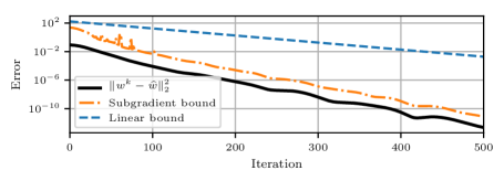
Figure 1: Comparison of the a-priori linear convergence bound (4) against the a-posteriori subgradient bound (5). Showing results over 500 iterations FISTA for the problem (7).

3 Upper-Level Problem

We now describe our algorithm for solving the upper-level problem of learning $\theta$. Suppose we have access to $n$ lower-level problems which depend on the same parameters $\theta\in\mathbb{R}^{m}$, and that each lower-level minimizer $\hat{w}_{j}(\theta)\in\mathbb{R}^{d_{j}}$ has an associated loss function $\ell_{j}:\mathbb{R}^{d_{j}}\to\mathbb{R}$; in Section 4, this will be a measure of test error. Then, our upper-level problem is

$$\min_{\theta\in\mathbb{R}^{m}} \>\>F(\theta):=\sum_{j=1}^{n}\ell_{j}(\hat{w}_{j}(\theta))+\mathcal{J}(\theta),\quad\text{subject to}\quad\hat{w}_{j}(\theta):=\operatorname*{arg\,min}_{w\in\mathbb{R}^{d}}\Phi_{j}(w,\theta),$$ (8)

where $\mathcal{J}(\theta)$ is an optional regularization term for $\theta$, and $\Phi_{j}$ is strongly convex in $w$ (but possibly nonsmooth) and smooth in $\theta$. Under these assumptions, there are various results showing that $\hat{w}_{j}(\theta)$ is locally Lipschitz in $\theta$ for a variety of problems; e.g. [Hintermüller and Wu(2015), Riis et al.(2018)Riis, Ehrhardt, Quispel, and Schönlieb].

To solve (8) we follow [Ehrhardt and Roberts(2020)] and use a model-based DFO method. Here, at every iteration $k$ we have a collection of points $\{y^{(k)}_{0},\ldots,y^{(k)}_{m}\}$ at which we have evaluated $\hat{w}_{j}$ (for each $j$), to some accuracy. We use this information to build a local quadratic model $m_{k}(\theta)$ which approximates $F(\theta)$ near $\theta^{(k)}$ by requiring that the model interpolate $F$ at each of $y^{(k)}_{0},\ldots,y^{(k)}_{m}$. Our upper-level iteration can be summarized as:

1. Build the interpolating local quadratic model $m_{k}(\theta)\approx F(\theta)$ using (inexact) evaluations of $\hat{w}_{j}(y^{(k)}_{0}),\ldots,\hat{w}_{j}(y^{(k)}_{m})$.

2. Calculate a minimizer $s^{(k)}$ of the model inside a trust region, namely solve (possibly inexactly) $\min_{\|s\|_{2}\leq\Delta_{k}}m_{k}(\theta^{(k)}+s)$, for a given trust-region radius $\Delta_{k}>0$.

3. Ensure $F(\theta^{(k)})$ and $F(\theta^{(k)}+s^{(k)})$ are evaluated to sufficiently high accuracy, and then if sufficient decrease is achieved, set $\theta^{(k+1)}=\theta^{(k)}+s^{(k)}$ and increase $\Delta_{k}$, otherwise set $\theta^{(k+1)}=\theta^{(k)}$ and decrease $\Delta_{k}$.

4. Replace one interpolation point with $\theta^{(k)}+s^{(k)}$.

This algorithm typically requires that our inexact lower-level evaluations $w_{j}(\theta)\approx\hat{w}_{j}(\theta)$ satisfy $\|w_{j}(\theta)-\hat{w}_{j}(\theta)\|_{2}\leq c\,\Delta_{k}^{2}$ for some $c>0$ (where we use $c=100$ in Section 4 below).

Full details of a suitable dynamic accuracy upper-level algorithm are given in [Ehrhardt and Roberts(2020)]. There, it is shown that, if $\mathcal{J}$, and each $\ell_{j}$ and $\Phi_{j}$ are sufficiently smooth, and each $\Phi_{j}$ is strongly convex in $w$, then the model-based DFO algorithm finds a $\theta$ with $\|\nabla F(\theta)\|_{2}\leq\epsilon$ in at most $\mathcal{O}(\epsilon^{-2})$ upper-level iterations, or at most $\mathcal{O}(\epsilon^{-2}|\log\epsilon|)$ lower-level iterations.

4 Numerical Results

Summary of Test Problem

We test our approach by attempting to learn elastic net regularizer [Zou and Hastie(2005)] weights $\theta\in\mathbb{R}^{2}$ for a logistic classifier of each digit 0–5 in MNIST [LeCun et al.(2010)LeCun, Cortes, and Burges] (i.e. each lower-level problem corresponds to a classifier for a different digit and the upper-level problem measures a test set error). Below, we validate the results of our approach by considering the remaining digits. To test our approach, we follow [Ehrhardt and Roberts(2020)] and use a version of DFO-LS [Cartis and Roberts(2019), Cartis et al.(2019)Cartis, Fiala, Marteau, and Roberts] which is modified to handle dynamic accuracy evaluations as per Section 3. We use FISTA (3) for the lower-level solver, and compare the dynamic accuracy approach with a combination of FISTA and DFO-LS, but using a fixed number of FISTA iterations $K$ for every lower-level solve. Full details are given in Appendix A.

General Comparison

Figure LABEL:fig_start0 compares the dynamic-accuracy variant against fixed-accuracy variants with low ($K=20$), medium ($K=200$) and high accuracy ($K=2000$), with upper-level initialization $\theta^{(0)}=[1,1]^{T}$ in all cases. Overall, dynamic accuracy is comparable to medium accuracy: it reaches the same $\theta$ at a similar speed. By comparison, low accuracy gives a quite different value of $\theta$ to the others, and high accuracy takes substantially more computational effort to converge. A key point to note here, is that dynamic accuracy performs similar to the best fixed-accuracy variant without requiring the necessary accuracy a priori.

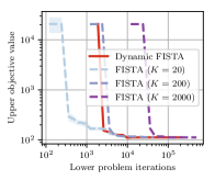
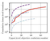
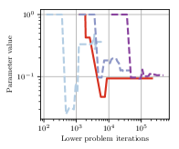
fig_start0[Objective $F(\theta)$] [FISTA iterations]   [Best $\ell_{1}$ penalty $10^{\theta_{1}}$] [Best $\ell_{2}$ penalty $10^{\theta_{2}}$]

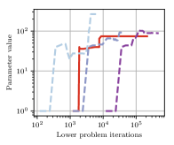
Figure 2: Initial results using $\theta^{(0)}=[1,1]^{T}$.

Robustness

It was observed in [Ehrhardt and Roberts(2020)] that dynamic accuracy is more robust to initialization and a good initialization can accelerate its initial objective decease. To test these features here, we perform the same tests as above, but vary the initial $\ell_{2}$ penalty by choosing $\theta^{(0)}_{2}\in\{-3,-2,\ldots,3\}$. Figure 3 shows that only high accuracy and dynamic accuracy give stable results, whereas the low and medium accuracy converge to different $\theta$ depending on the starting point. Figure 4 shows that as $\theta^{(0)}_{2}$ increases, the relative performance of dynamic accuracy improves. Thus, since dynamic accuracy is stable with respect to initialization, selecting $\theta^{(0)}$ to give well-conditioned lower-level problems is appropriate and the associated reduction in computational work can be achieved.

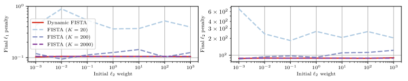
Figure 3: Final values of $\theta_{1}$ (left) and $\theta_{2}$ (right) reached for different starting points $\theta^{(0)}_{2}$.

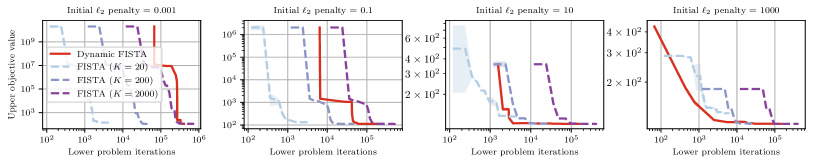
Figure 4: Comparison of objective reduction for different choices of starting point $\theta^{(0)}_{2}$.

Validation

Finally, we measure the generalizability of the upper-level minimizers. Here, the learned values of $\theta$ from each accuracy variant and each initialization $\theta^{(0)}$ are used to train logistic classifiers for MNIST (using a new set of 5000 training images), and measure their test error (on another new set of 1000 test images). Despite the upper-level problem only considering digits 0–5, here we look at the performance of each $\theta$ in training classifiers for all digits. We measure the test error by looking at the proportion of test images classified correctly (using the predictor $\hat{y}^{(j)}_{i}=1$ if $p^{(j)}_{i}(\hat{w}_{j}(\theta))\geq 0.5$; see Appendix A). Figure 5 shows the validation for each digit $j\in\{0,\ldots,9\}$ and initialization $\theta^{(0)}_{2}$. The overall accuracy is generally lower for digits 6–9 than the digits used in the upper-level objective (0–5). However, we see consistently that dynamic and high accuracy achieve better prediction accuracy than low and medium accuracy.

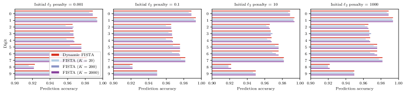
Figure 5: Comparison of validation results for different choices of starting point $\theta^{(0)}_{2}$.

5 Conclusions and Further Work

We have extended the approach in [Ehrhardt and Roberts(2020)] to the case of nonsmooth lower-level problems—we can guarantee solutions to the lower-level problem are sufficiently accurate for the upper-level algorithm. When applied to learning elastic net regularizer weights for MNIST, we find that the dynamic accuracy DFO approach gives a robust method for hyperparameter tuning. Compared to the fixed-accuracy variants, which have strong dependency on the selected number of iterations (both in computational speed and quality of minimizer), the dynamic-accuracy version can achieve both fast progress and high-quality minimizers, without needing to be manually tuned. We delegate to future work a full study of the convergence of the upper-level algorithm in this setting, and comparisons between the dynamic accuracy DFO approach and other methods for hyperparameter tuning.

5.1 Acknowledgements

MJE acknowledges support from the EPSRC (EP/S026045/1, EP/T026693/1), the Faraday Institution (EP/T007745/1) and the Leverhulme Trust (ECF-2019-478).

Appendix A Details of Numerical Test Model

General Problem Formulation

In this work, we focus on a specific choice of problem, namely selecting regularizer weights for logistic regression [Murphy(2012), Chapter 8]. Specifically, for upper-level problem $j\in\{1,\ldots,n\}$, suppose we have training pairs $\{(x^{(j)}_{i},y^{(j)}_{i})\}_{i=1}^{N_{j}}$ with features $x^{(j)}_{i}\in\mathbb{R}^{d_{j}}$ and binary labels $y^{(j)}_{i}\in\{-1,1\}$. Minimizing the negative log-likelihood of the corresponding logistic classifier, with an elastic net regularizer [Zou and Hastie(2005)], corresponds to the lower-level problem

$$\hat{w}_{j}(\theta):=\operatorname*{arg\,min}_{w\in\mathbb{R}^{d_{j}}}\Phi_{j}(w,\theta):=\frac{1}{N_{j}}\sum_{i=1}^{N_{j}}\log(1+\exp(-y^{(j)}_{i}w^{T}x^{(j)}_{i}))+\frac{10^{\theta_{1}}}{2}\|w\|_{2}^{2}+10^{\theta_{2}}\|w\|_{1},\quad$$ (9)

for (undetermined) regularizer log-weights $\theta_{1},\theta_{2}\in\mathbb{R}$. That is, we form $\Phi_{j}(w,\theta)$ (2) by taking

$$f_{j}(w,\theta):=\frac{1}{N_{j}}\sum_{i=1}^{N_{j}}\log(1+\exp(-y^{(j)}_{i}w^{T}x^{(j)}_{i}))+\frac{10^{\theta_{1}}}{2}\|w\|_{2}^{2},\quad\text{and}\quad g_{j}(w,\theta):=10^{\theta_{2}}\|w\|_{1},$$ (10)

and so $f_{j}(\cdot,\theta)$ is $\mu_{j}(\theta)$-strongly convex and $L_{j}(\theta)$-smooth with

$$\mu_{j}(\theta):=10^{\theta_{1}},\quad\text{and}\quad L_{j}(\theta):=\frac{1}{4N_{j}}\|X^{(j)}\|_{2}^{2}+10^{\theta_{1}},$$ (11)

where $X^{(j)}\in\mathbb{R}^{{N_{j}}\times{d_{j}}}$ has columns $x^{(j)}_{i}$.

As our upper-level objective, suppose for each lower-level problem $j$ we have learned weights $w_{j}(\theta)\in\mathbb{R}^{d_{j}}$ (in practice $w_{j}(\theta)$ is our approximation to $\hat{w}_{j}(\theta)$ from solving (9) to some finite accuracy). We then suppose we have a test set $\{(\widetilde{x}^{(j)}_{i},\widetilde{y}^{(j)}_{i})\}_{i=1}^{\widetilde{N}_{j}}$, and we calculate the estimated probabilities $p^{(j)}_{i}(\hat{w}_{j}(\theta))=\operatorname{sigm}(\hat{w}_{j}(\theta)^{T}\widetilde{x}^{(j)}_{i})$ is the probability that $\widetilde{y}^{(j)}_{i}=1$ as determined by the classifier. We then take our loss for the lower-level problem $j$ to be a smoothed approximation of the test accuracy:

$$\ell_{j}(\hat{w}_{j}(\theta)):=\sum_{i=1}^{\widetilde{N}_{j}}\left[p^{(j)}_{i}(\hat{w}_{j}(\theta))-\widetilde{p}^{(j)}_{i}\right]^{2},\qquad\text{where}\qquad\widetilde{p}^{(j)}_{i}=\begin{cases}1,&\widetilde{y}^{(j)}_{i}=1,\\ 0,&\text{otherwise}.\end{cases}$$ (12)

That is, $\ell_{j}(\theta)$ is the squared Euclidean distance from the vector $[p^{(j)}_{1},\ldots,p^{(j)}_{\widetilde{N}_{j}}]^{T}$ to the ‘perfect’ classifier’s probabilities $[\widetilde{p}^{(j)}_{1},\ldots,\widetilde{p}^{(j)}_{\widetilde{N}_{j}}]^{T}$.

Example Problem

We take our training data from MNIST [LeCun et al.(2010)LeCun, Cortes, and Burges], where we attempt to learn a classifier for each digit separately (i.e. for digit $j\in\{0,\ldots,9\}$, learn a classifier for whether image $i$ is of digit $j$ or not). In this case, we have the same features for all lower-level problems, and we choose $N_{j}=5000$ and $\widetilde{N}_{j}=1000$ images for the training and test sets respectively. To test the generalizability of our approach, we only solve the upper-level problem for digits 0–5 (i.e. $n=6$). We validate the final learned $\theta$ on the same problem for the remaining digits 6–9.

We augment our upper-level problem with a regularizer which encourages well-conditioned lower-level problems and a large value of $\theta_{2}$ (which should yield sparse weights $w_{j}$):

$$\mathcal{J}(\theta):=\alpha_{1}\left(\frac{L(\theta)}{\mu(\theta)}\right)^{2}+\alpha_{2}10^{-\theta_{2}},$$ (13)

for weights $\alpha_{1}=10^{-8}$ and $\alpha_{2}=1$.

To test our approach, we follow [Ehrhardt and Roberts(2020)] and use a version of DFO-LS [Cartis and Roberts(2019), Cartis et al.(2019)Cartis, Fiala, Marteau, and Roberts] which is modified to handle dynamic accuracy evaluations as per Section 3. We use FISTA (3) for the lower-level solver, and compare the dynamic accuracy approach with a combination of FISTA and DFO-LS, but using a fixed number of FISTA iterations $K$ for every lower-level solve. We impose bounds $\theta\in[10^{-8},10^{8}]^{2}$, and terminate after 80 upper-level evaluations or the trust-region radius in DFO-LS reaches $10^{-5}$.

References

- [Arridge et al.(2019)Arridge, Maass, Öktem, and Schönlieb] Simon Arridge, Peter Maass, Ozan Öktem, and Carola-Bibiane Schönlieb. Solving inverse problems using data-driven models. Acta Numerica, 28:1–174, 2019.
- [Audet and Hare(2017)] Charles Audet and Warren Hare. Derivative-Free and Blackbox Optimization. Springer Series in Operations Research and Financial Engineering. Springer, Cham, Switzerland, 2017.
- [Beck(2017)] Amir Beck. First-Order Methods in Optimization, volume 25 of MOS-SIAM Series on Optimization. MOS/SIAM, Philadelphia, 2017.
- [Beck and Teboulle(2009)] Amir Beck and Marc Teboulle. A fast iterative shrinkage-thresholding algorithm. SIAM Journal on Imaging Sciences, 2(1):183–202, 2009.
- [Benning and Burger(2018)] Martin Benning and Martin Burger. Modern regularization methods for inverse problems. Acta Numerica, 27:1–111, 2018.
- [Cartis and Roberts(2019)] Coralia Cartis and Lindon Roberts. A derivative-free Gauss-Newton method. Mathematical Programming Computation, 11(4):631–674, 2019.
- [Cartis et al.(2019)Cartis, Fiala, Marteau, and Roberts] Coralia Cartis, Jan Fiala, Benjamin Marteau, and Lindon Roberts. Improving the flexibility and robustness of model-based derivative-free optimization solvers. ACM Transactions on Mathematical Software, 45(3):32:1–32:41, 2019.
- [Chambolle and Pock(2016)] Antonin Chambolle and Thomas Pock. An Introduction to Continuous Optimization for Imaging. Acta Numerica, 25:161–319, 2016.
- [Chen et al.(2018)Chen, Menickelly, and Scheinberg] Ruobing Chen, Matt Menickelly, and Katya Scheinberg. Stochastic optimization using a trust-region method and random models. Mathematical Programming, 169(2):447–487, 2018.
- [Conn et al.(2009)Conn, Scheinberg, and Vicente] Andrew R. Conn, Katya Scheinberg, and Luís N. Vicente. Introduction to Derivative-Free Optimization, volume 8 of MPS-SIAM Series on Optimization. MPS/SIAM, Philadelphia, 2009.
- [Ehrhardt and Roberts(2020)] Matthias J. Ehrhardt and Lindon Roberts. Inexact derivative-free optimization for bilevel learning. arXiv preprint arXiv:2006.12674, 2020.
- [Engl et al.(1996)Engl, Hanke, and Neubauer] H. W. Engl, M. Hanke, and A. Neubauer. Regularization of Inverse Problems. Mathematics and Its Applications. Springer, 1996.
- [Feurer and Hutter(2019)] Matthias Feurer and Frank Hutter. Hyperparameter optimization. In Frank Hutter, Lars Kotthoff, and Joaquin Vanschoren, editors, Automated Machine Learning: Methods, Systems, Challenges, pages 3–33. Springer, Cham, Switzerland, 2019.
- [Garmanjani et al.(2016)Garmanjani, Júdice, and Vicente] R. Garmanjani, Diogo Júdice, and Luís N. Vicente. Trust-region methods without using derivatives: Worst case complexity and the nonsmooth case. SIAM Journal on Optimization, 26(4):1987–2011, 2016.
- [Ghanbari and Scheinberg(2017)] Hiva Ghanbari and Katya Scheinberg. Black-box optimization in machine learning with trust region based derivative free algorithm. arXiv preprint arXiv:1703.06925, 2017.
- [Grapiglia et al.(2016)Grapiglia, Yuan, and Yuan] Geovani Nunes Grapiglia, Jinyun Yuan, and Ya-xiang Yuan. A derivative-free trust-region algorithm for composite nonsmooth optimization. Computational and Applied Mathematics, 35(2):475–499, 2016.
- [Hansen(1992)] Per Christian Hansen. Analysis of Discrete Ill-Posed Problems by Means of the L-Curve. SIAM Review, 34(4):561–580, 1992.
- [Hintermüller and Wu(2015)] Michael Hintermüller and Tao Wu. Bilevel optimization for calibrating point spread functions in blind deconvolution. Inverse Problems and Imaging, 9(4):1139–1169, 2015.
- [Khan et al.(2018)Khan, Larson, and Wild] Kamil A. Khan, Jeffrey Larson, and Stefan M. Wild. Manifold sampling for optimization of nonconvex functions that are piecewise linear compositions of smooth components. SIAM Journal on Optimization, 28(4):3001–3024, 2018.
- [Kunisch and Pock(2013)] Karl Kunisch and Thomas Pock. A Bilevel Optimization Approach for Parameter Learning in Variational Models. SIAM Journal on Imaging Sciences, 6(2):938–983, 2013.
- [Lakhmiri et al.(2019)Lakhmiri, Le Digabel, and Tribes] Dounia Lakhmiri, Sébastien Le Digabel, and Christophe Tribes. HyperNOMAD: Hyperparameter optimization of deep neural networks using mesh adaptive direct search. Technical Report G-2019-46, HEC Montréal, 2019.
- [LeCun et al.(2010)LeCun, Cortes, and Burges] Yann LeCun, Corinna Cortes, and CJ Burges. Mnist handwritten digit database. ATT Labs [Online]. Available: http://yann.lecun.com/exdb/mnist, 2, 2010.
- [Li et al.(2018)Li, Jamieson, DeSalvo, Rostamizadeh, and Talwalkar] Lisha Li, Kevin Jamieson, Giulia DeSalvo, Afshin Rostamizadeh, and Ameet Talwalkar. Hyperband: A novel bandit-based approach to hyperparameter optimization. Journal of Machine Learning Research, 18(4):1–52, 2018.
- [Luketina et al.(2016)Luketina, Berglund, Greff, and Raiko] Jelena Luketina, Mathias Berglund, Klaus Greff, and Tapani Raiko. Scalable gradient-based tuning of continuous regularization hyperparameters. In Proceedings of the 33rd International Conference on Machine Learning, New York, USA, 2016.
- [Murphy(2012)] Kevin P. Murphy. Machine Learning: A Probabilistic Perspective. The MIT Press, Cambridge, 2012.
- [Ochs et al.(2015)Ochs, Ranftl, Brox, and Pock] Peter Ochs, René Ranftl, Thomas Brox, and Thomas Pock. Bilevel Optimization with Nonsmooth Lower Level Problems. In SSVM, volume 9087, pages 654–665, 2015.
- [Riis et al.(2018)Riis, Ehrhardt, Quispel, and Schönlieb] Erlend S. Riis, Matthias J. Ehrhardt, G. R. W. Quispel, and Carola-Bibiane Schönlieb. A geometric integration approach to nonsmooth, nonconvex optimisation. arXiv preprint arXiv:1807.07554, 2018.
- [Shaban et al.(2019)Shaban, Cheng, Hatch, and Boots] Amirreza Shaban, Ching-An Cheng, Nathan Hatch, and Byron Boots. Truncated back-propagation for bilevel optimization. Proceedings of Machine Learning Research, 89:1723–1732, 2019.
- [Sherry et al.(2020)Sherry, Benning, los Reyes, Graves, Maierhofer, Williams, Schönlieb, and Ehrhardt] Ferdia Sherry, Martin Benning, Juan Carlos De los Reyes, Martin J. Graves, Georg Maierhofer, Guy Williams, Carola-Bibiane Schönlieb, and Matthias J. Ehrhardt. Learning the sampling pattern for MRI. IEEE Transactions on Medical Imaging, 2020.
- [Zou and Hastie(2005)] Hui Zou and Trevor Hastie. Regularization and variable selection via the elastic net. Journal of the Royal Statistical Society Series B, 67(2):301–320, 2005.