Fuzzy measurements and coarse graining in quantum many-body systems

Abstract

Using the quantum map formalism, we provide a framework to construct fuzzy and coarse grained quantum maps of many-body systems that account for limitations in the resolution of real measurement devices probing them. The first set of maps handles particle-indexing errors, while the second deals with the effects of detectors that can only resolve a fraction of the system constituents. We apply these maps to a spin-$1/2$ $XX$-chain obtaining a blurred picture of the entanglement generation and propagation in the system. By construction, both maps are simply related via a partial trace, which allows us to concentrate on the properties of the former. We fully characterize the fuzzy map, identifying its symmetries and invariant spaces. We show that the volume of the tomographically accessible states decreases at a double-exponential rate in the number of particles, imposing severe bounds on the ability to read and use information of a many-body quantum system.

I Introduction

Ultimately, like with all systems in nature, limitations in measurements set the boundaries of what we can learn about the quantum world. Not surprisingly, the measurement problem has played a prominent role in quantum mechanics since its foundation [1]. Nowadays, quantum many-body systems can be probed and manipulated at the single-particle level [2], allowing for the study with unprecedented detail of problems ranging from quantum entanglement to thermalization [3]. Such dazzling advances in recent years have been possible due to an unparalleled development of measurement techniques [2, 4] as well as of our understanding of the measurement process in quantum mechanics [5, 6]. Yet, with the advent of quantum technologies, technical and conceptual challenges remain.

Prominently, the scalability required for quantum technology places great demands on the measurement and control of quantum systems with an increasing number of degrees of freedom. At present, the necessary resources for the experimental manipulation and characterization of many-body quantum systems at the single particle level swiftly mount up with the size of the system [7, 8], making such detailed description unfeasible. A technical obstacle that evinces the pressing necessity of an accurate effective characterization of these systems when probed with the use of imperfect measuring devices. In this work, invoking the language of quantum channels, we construct a framework to study this emerging portrayal of many-body systems.

Imperfect measurements were considered by Peres, when assessing the consequences of having an experimental uncertainty in the eigenvalue measurement larger than the difference between consecutive eigenvalues [9]. In this context, projective measurements were generalized to positive operator valued measurements, allowing for a more gentle effect on the measured system [10] and incorporating unsharp, weak, and fuzzy measurement schemes [11, 12, 13]. More recently, as an alternative to the decoherence program, in [14] and [15] it has been argued that classical features emerge from coarse grained descriptions of quantum systems when measured with imperfect apparatuses, sparking research on ad hoc models to estimate the resilience of quantum features under imperfect measurements [16, 17, 18], arguably, an additional issue to account for in the development of quantum technologies [8].

This progress notwithstanding, a solid framework that can systematically address the implications of studying quantum many-body systems using imperfect measurements is still lacking. This work aims at closing this gap. Our formalism considers imperfect detection of two different, but deeply related, kinds in quantum many-body systems: fuzzy measurements (FMs), in which single particles can be resolved, however, there is always a finite probability of their misidentification; and coarse graining (CG) measurements, in which groups of particles are treated collectively as an effective particle, either because the measurement device is not sensible enough to resolve all degrees of freedom in the system, or because only a few of these degrees of freedom are of relevance for the system property being studied. We formalize both concepts in the language of quantum maps, identifying their symmetries, spectra, and invariant spaces. Physical consequences of our results are illustrated with spin-entanglement waves, in which a blurring of the observable entanglement is observed, and a study of the contractive properties of our maps, showing a double-exponential contraction rate of the accessible state volume with the number of particles, a remarkable result hinting at the fragility of quantum resources with respect to imperfect measurements.

II Fuzzy measurements

Consider the situation in which a single-particle measurement is performed on a many-body system, but one is not sure on which particle this measurement was applied. For example, one shines an ion chain, and obtains a fluorescent signal. However, due to the addressing imperfections of the detector device, one is not able to determine the exact origin of the fluorescent signal. The obtained information in this case becomes blurred, yet its quantification is still possible.

Consider first the simplest many-body system: two particles. Suppose a measurement of the observable $A\otimes B$ in a two particle system is wanted. Yet, with probability $1-p$, the measurement apparatus mistakes the particles, so instead, sometimes, a measurement of $B\otimes A$ is done. Hence, if $\rho$ is the state of the system, the outcome of this FM is

$$p\mathop{\mathrm{Tr}}\nolimits\rho A\otimes B+(1-p)\mathop{\mathrm{Tr}}\nolimits\rho B\otimes A=\langle A\otimes B\rangle_{\mathcal{F}_{2\text{p}}[\rho]},$$ (1)

with $\mathcal{F}_{2\text{p}}[\rho]=p\rho+(1-p)S_{01}[\rho]$, where the brackets in front of a unitary operator denote its natural action on density matrices, e.g. $S_{ij}[\rho]=S_{ij}\rho S_{ij}^{\dagger}$ is the application of the swap gate with respect to particles $i$ and $j$ to the system state. Incidentally, note that if the error is assumed to be the same for every observable of the system, then $\mathcal{F}_{2\text{p}}[\rho]$ corresponds to the tomographically accessible state .

The simple reasoning above can be followed for an $n$-body system. If the measurement device wrongly identifies particles with probability $p_{P}\geq 0$, according to permutation $P$, the outcome of the FM of operator $M$ is $\mathop{\mathrm{Tr}}\nolimits\left(M\mathcal{F}[\rho]\right)$, with

$$\mathcal{F}[\rho]=\sum_{P\in\mathcal{S}}p_{P}P[\rho],$$ (2)

where $\mathcal{S}$ is a subset of the symmetric group of $n$ particles, and $\sum_{P\in\mathcal{S}}p_{P}=1$. We regard Eq. (2) as the most general form of the FM channel and consider some particular examples below.

Quite generally, during a measurement, two-body errors are more likely to occur than higher order ones. Accounting just for these, the effective tomographically accessible state is

$$\mathcal{F}_{2\text{b}}[\rho]=p\rho+(1-p)\sum_{i,j}p_{ij}S_{ij}[\rho],$$ (3)

with $\mathcal{S}$ containing only swaps. A relevant related case is a periodic one-dimensional chain in which errors between adjacent particles are the only ones taken into account. In this case

$$\mathcal{F}_{1\text{d}}[\rho]=p\rho+(1-p)\sum_{i}p_{i}S_{i,i+1}[\rho]$$ (4)

with $\mathcal{S}$ consisting of neighboring exchanges.

Similar considerations can be done for two-dimensional systems or more refined proposals, e.g. a swap probability that decays with the distance between $i$ and $j$, or a particular experimental setup.

III Coarse graining

Consider now a slightly worse situation in which the measurement device is unable to resolve the fine details of the whole system and is forced to capture effective reduced states of randomly chosen subsets of the system. Two processes characterize such an apparatus: the choice of random subsets and the reduction to a representative state as a result of a partial trace of the subset. The latter accounts for the discarded information of the inaccessible parts and provides a coarse-grained picture of the system state. This is illustrated in the simple case of a two-particle system. The expected value of the single-particle observable $M$ measured by an apparatus that with probability $p$ ($1-p$) detects the first (second) particle is $\mathop{\mathrm{Tr}}\nolimits\left(M\rho_{\text{eff}}\right)$, with the effective single-particle state $\rho_{\text{eff}}=\mathop{\mathrm{Tr}}\nolimits_{1}\mathcal{F}_{2\text{p}}[\rho]$ [cf. eq. (1)].

The same procedure can be applied to systems with more than two particles. Assume that a detector is able to measure only $N$ particles at a time, picking each one of them randomly from subsets of $m_{k}$ particles, with $k=1,\dots,N$. The effective $N$-particle state is given by

$$\rho_{\text{eff}}:=\left(\bigotimes_{k=1}^{N}\mathcal{C}_{m_{k}}\right)[\rho]$$ (5)

with

$$\mathcal{C}_{m}[\rho]=\frac{1}{m}\mathop{\mathrm{Tr}}\nolimits_{\overline{1}}\sum_{i=1}^{m}S_{1,i}[\rho],$$ (6)

where the overline in the subindex of the trace denotes the set complement, in this case trace over all but the first particle. As we now show, this channel is the composition of a FM and a partial trace: a consequence of the linearity of the trace and the group properties of permutations. Let us start by factorizing the partial traces in a tensor product, as their domains are disjoint. Noting that $\mathcal{F}^{(m)}[\rho]:=1/m\sum_{i=1}^{m}S_{1,i}[\rho]$ is a fuzzy map, we can write

$$\begin{split}\bigotimes_{k=1}^{N}\mathcal{C}_{m_{k}}&=\mathop{\mathrm{Tr}}\nolimits^{(1)}_{\overline{1}}\otimes\dots\otimes\mathop{\mathrm{Tr}}\nolimits^{(N)}_{\overline{1}}\left(\mathcal{F}^{(m_{1})}\otimes\dots\otimes\mathcal{F}^{(m_{N})}\right)\\ &=\mathop{\mathrm{Tr}}\nolimits_{\overline{\left\{1_{1},\dots,1_{N}\right\}}}\left(\mathcal{F}^{(m_{1})}\otimes\dots\otimes\mathcal{F}^{(m_{N})}\right).\end{split}$$ (7)

Now, by distributing the tensor product, we can define the FM

$$\mathcal{F} :=\mathcal{F}^{(m_{1})}\otimes\dots\otimes\mathcal{F}^{(m_{N})}$$

$$=\left(\frac{1}{m_{1}}\sum_{i_{1}=1}^{m_{1}}S_{1,i_{1}}\right)\otimes\dots\otimes\left(\frac{1}{m_{N}}\sum_{i_{N}=1}^{m_{N}}S_{1,i_{N}}\right)$$

$$=\prod_{j=1}^{N}\frac{1}{m_{j}}\sum_{i_{1},\dots,i_{N}=1}^{m_{1},\dots,m_{N}}S_{1,i_{1}}\otimes\dots\otimes S_{1,i_{N}},$$

since tensor products of swaps result in disjoint permutations with respect to particle sets. We can now rewrite the effective $N$-particle state as the result of applying the CG map to $\rho$,

$$\rho_{\text{eff}}:=\mathop{\mathrm{Tr}}\nolimits_{\kappa}\mathcal{F}[\rho],$$ (8)

where $\kappa$ is a suitable choice of subsystem to trace, as given in (7). The case $m_{k}=m=3$ is depicted in fig. 1(a).

Motivated by a different physical feasible situation, we examine a second CG measurement with its corresponding FM. Consider a chain of particles such that the conditions with respect to the measurement device alternate, e.g. the even ones are closer to the detector than the odd ones; see fig. 1(b) for an example. Assume that with probability $p$ the measurement device measures the even particles, but with a position dependent probability one of its odd-labeled neighbors is detected. The channel associated with such a measurement is

$$p\mathop{\mathrm{Tr}}\nolimits_{\text{odd}}\rho+(1-p)\mathop{\mathrm{Tr}}\nolimits_{\text{odd}}\sum_{i}p_{i}S_{i,i+1}[\rho]=\mathop{\mathrm{Tr}}\nolimits_{\text{odd}}\mathcal{F}_{1\text{d}}[\rho].$$ (9)

Single particle observables of, say, particle $2i$ are evaluated with respect to the effective density matrix $[1+p(p_{2i-1}+p_{2i})]\rho_{2i}+pp_{2i-1}\rho_{2i-1}+pp_{2i}\rho_{2i+1}$, where $\rho_{i}$ is the reduced density matrix for particle $i$. Two particle observables, say of particles $2i$ and $2j$, are calculated with a density matrix, with coefficients of order $0$ in $1-p$ of $\rho_{2i,2j}$, and other contributions of order $1$, of $\rho_{2i\pm 1,2j}$ and $\rho_{2i,2j\pm 1}$.

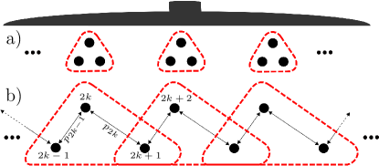
Figure 1: CG schemes. (a) The detector groups sets of $m=3$ particles into one; see eq. (6). (b) The detector measures even particles with a higher probability than odd ones, but sometimes it mistakes them for one of their neighbors.

The above examples illustrate how to construct reduced quantum states using quantum maps motivated by probabilistically chosen subsystems, based on the physical arrangement of both the system and the measurement device; this construction might include the simultaneous exchange of a greater number of particles. An encompassing scheme for CG maps is

$$\mathcal{C}[\rho] =\mathop{\mathrm{Tr}}\nolimits_{\tau}\sum_{P\in\mathcal{S}}p_{P}P\rho P^{\dagger}{}=\mathop{\mathrm{Tr}}\nolimits_{\tau}\mathcal{F}[\rho],$$ (10)

where $\tau$ denotes the part of the system that is traced.

IV Fuzzy and coarse grained entanglement waves

To illustrate the use of the proposed maps, we now consider the recently achieved observation of single spin impurity dynamics [20] and spin-entanglement wave propagation [21] in one-dimensional Bose-Hubbard chains at the level of single-atom-resolution detection [22, 23].

The dynamics of a single spin impurity in a one dimensional homogeneous spin-$1/2$ $XX$-chain is generated by the Hamiltonian $\hat{H}=-J_{\text{ex}}\sum_{j}(\hat{\sigma}^{+}_{j}\hat{\sigma}^{-}_{j+1}+\hat{\sigma}^{-}_{j}\hat{\sigma}^{+}_{j+1})$, where $J_{\text{ex}}$ is the exchange coupling and $\hat{\sigma}^{\pm}_{j}$ are spin-$1/2$ raising (lowering) operators acting on particle $j$ [24, 25]. We write an infinite spin-chain state with a single spin-up impurity at site $j$ as ${|j\rangle}\equiv{|\dots,0_{j-1},1_{j},0_{j+1},\dots\rangle}$, where ${|1\rangle}$ (${|0\rangle}$) refers to spin a spin-up (spin-down) state in the $z$ basis, and choose the initial state as ${|0\rangle}$, i.e., with the spin-up impurity at the center of the chain. At later times the excitation travels coherently to both sides of the chain as described by the state of the system ${|\psi(t)\rangle}=\sum_{j}\phi_{j}(t){|j\rangle}$, where $\phi_{j}(t)=\mathrm{i}^{j}J_{j}(tJ_{\text{ex}}/\hbar)$ with $J_{j}(x)$ the Bessel function of the first kind [26]. In the first column in fig. 2, the generation of concurrence and its spread in a wave-like fashion along the spin chain is shown [25, 24, 27]. It is noticeable how the maximum of the concurrence propagates to neighboring sites, moving away from the center.

We now study the entanglement in the system under FM. Assume, that with probability $1-p$, the measurement apparatus is displaced equiprobably one site to the right or to the left of the chain. This case is described by eq. (2) with $\mathcal{S}=\{\openone,T,T^{\dagger}\}$, and $T|j\rangle=|j+1\rangle$, $p_{\openone}=p$, $p_{T}=p_{T^{\dagger}}=(1-p)/2$. As shown in the second column of fig. 2, the entanglement still exhibits its wavelike spreading albeit with a weaker intensity compared to the unaltered dynamics. This decoherence effect of the FM is responsible for the blurry appearance of the images, which however is not homogeneous, and is most prominent among distant symmetric pairs. Observe, for instance, that the squarelike structures that can be seen for the exact dynamics at $t=6$ are almost completely lost when the FM is applied.

We also consider the effects of CG. For this, we group the particles in disjoint sets, as in eq. (6). To respect the symmetry $j\to-j$ of the system, we group particles in sets of two ($\pm\{1,2\},\pm\{3,4\},\ldots$), with $\mathcal{C}_{2}$, and sets of four ($\pm\{1,2,3,4\},\pm\{5,6,7,8\},\ldots$), with $\mathcal{C}_{4}$, leaving particle $j=0$ unaltered. The entanglement evolution for these two cases is shown in columns $3$ and $4$ in fig. 2 for $\mathcal{C}_{2}$ and $\mathcal{C}_{4}$, respectively. In both cases, despite the lower resolution, the entanglement wavelike propagation can still be seen, with a higher intensity for $\mathcal{C}_{2}$ than for $\mathcal{C}_{4}$. Interestingly, entanglement seems to be suppressed more for neighboring particles than for distant CG particles. This can be appreciated in the last two columns in fig. 2, where the pattern is concentrated along the diagonal.

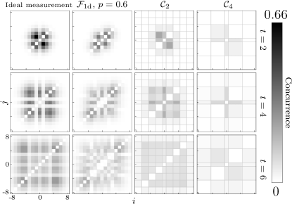
Figure 2: Concurrence for the single spin impurity dynamics as a function of lattice sites $i$ and $j$ at different times. The first column shows the entanglement for the unaltered states. The second column corresponds to an FM, whereas the third and fourth columns display results for coarse-grained descriptions, grouping two and four particles, respectively (gridlines group the coarse-grained sets of particles). The central particle has not been coarse grained in order to maintain the symmetry.

V Symmetries and spectrum

V.1 Symmetries of fuzzy measurements

Understanding the symmetries of a physical system is crucial to understanding its dynamics. For closed quantum systems symmetries result in quantum numbers, which are used to understand and classify the system’s spectrum. Here, we calculate all symmetries for generic FMs, i.e., with $p_{P}>0$ for every permutation $P$ in the symmetric group, and, as an important example, connect them with the generic invariant space.

Consider a system of $n$ particles with a single-particle space of dimension $d$. We start by introducing the linear superoperator $\Gamma_{l,l^{\prime}}[\varrho]=\gamma_{l,l^{\prime}}\varrho$, which counts how many particles in $\varrho$ are in $|l\rangle\langle l^{\prime}|$. For example, for $\varrho=|00\rangle\langle 01|=|0\rangle\langle 0|\otimes|0\rangle\langle 1|$, $\Gamma_{0,0}[\varrho]=\Gamma_{0,1}[\varrho]=\varrho$ while $\Gamma_{1,0}[\varrho]=\Gamma_{1,1}[\varrho]=0$. Clearly, operators $\Gamma_{l,l^{\prime}}$ commute among themselves. In addition, for any particle permutation, $\Gamma_{l,l^{\prime}}P[\varrho]=P\Gamma_{l,l^{\prime}}[\rho]$, and therefore they also commute with the FM, $[\mathcal{F},\Gamma_{l,l^{\prime}}]=0$. Hence $\mathcal{F}$ can be diagonalized in blocks $\mathcal{F}_{\gamma}$, each indexed by a matrix $\gamma$ with $d\times d$ integers ranging from 0 to $n$. The subspace of physical states is the one labeled by all diagonal $\gamma$s. The number of blocks can be counted using the stars and bars theorem [28] and is given by the binomial coefficient $\binom{d^{2}+n-1}{n}$. Since the total number of particles is fixed, $\sum_{l,l^{\prime}}\gamma_{l,l^{\prime}}=n$ in all blocks.

Note that there are some equivalent blocks. Working in the computational basis, it can be shown by explicit substitution that if $\Gamma_{l,l^{\prime}}[\varrho]=\gamma_{l,l^{\prime}}\varrho$, then $\Gamma_{l^{\prime},l}[\varrho^{\text{T}}]=\gamma_{l^{\prime},l}\varrho^{\text{T}}$, and that

$$(\varrho_{1},\mathcal{F}[\varrho_{2}])=(\varrho_{1}^{\text{T}},\mathcal{F}[\varrho_{2}^{\text{T}}]),$$ (11)

for arbitrary $\varrho_{1}$ and $\varrho_{2}$. Both identities combined lead to $\mathcal{F}_{\gamma}=\mathcal{F}_{\gamma^{T}}$ when an appropriate order of the computational basis is used. Further block equivalences follow from relabeling symmetries of the levels that allow block identification. Let $Q$ be any of the $d!$ unitary operators that relabels the elements of the computational basis; for qubits this set is $\{\openone,\sigma_{x}^{\otimes n}\}$. Since $[Q,P]=0$, $\forall P\in\mathcal{S}$, it follows that

$$(\rho_{1},\mathcal{F}[\rho_{2}])=(Q\rho_{1}Q^{\prime},\mathcal{F}[Q\rho_{2}Q^{\prime}]),$$ (12)

for arbitrary $\varrho_{1}$ and $\varrho_{2}$, establishing the equivalence between block $\mathcal{F}_{M(Q)\gamma M(Q^{\prime})^{\text{T}}}$ and block $\mathcal{F}_{\gamma}$, with $M(Q)$ the permutation matrix of $d$ elements associated with $Q$.

Examining the qubit case provides some intuition in the interpretation of matrix $\gamma$. For qubits, $\gamma$ is a $2\times 2$ matrix whose integer, semipositive entries should add up to $n$. This leaves three free parameters, which we organize as follows: $\alpha=\gamma_{1,0}+\gamma_{1,1}$ and $\beta=\gamma_{0,1}+\gamma_{1,1}$ which count the number of excitations in the ket and in the bra, respectively, and $\gamma_{1,1}$. Thanks to the identification of blocks, we can always choose $\alpha,\beta,\gamma\leq n/2$, and the degeneracy $\delta$ depends on the repeated values of the entries of $\gamma$. Thus, we can write

$$\mathcal{F}^{\text{qubits}}=\bigoplus_{\alpha,\beta,\gamma_{1,1}=0}^{\lfloor n/2\rfloor}\mathcal{F}_{(\alpha,\beta,\gamma_{1,1})}^{\oplus\delta(\gamma)}.$$

For the generic case the blocks $\mathcal{F}_{\gamma}$ are irreducible. To prove it, note that if all elements of the permutation group in $\mathcal{F}$ have a positive weight, all matrix elements of $\mathcal{F}_{\gamma}$ in the computational basis of the corresponding subspace are strictly positive. This is a consequence of the fact that for any two such basis elements $\varrho_{1,2}$, characterized by the same $\gamma$, there exists a permutation $P$ such that $P[\varrho_{1}]=\varrho_{2}$; see Appendix A. Therefore the blocks $\mathcal{F}_{\gamma}$ are irreducible [29]. Moreover, according to the Perron-Frobenius theorem [30], each one contains only one invariant matrix. This implies that for diagonal $\gamma$, the blocks $\mathcal{F}_{\gamma}$ define ergodic quantum channels [31].

V.2 Invariant space of fuzzy measurements

Due to the Perron-Frobenius theorem and the total of irreducible blocks in the generic case, it follows immediately that the dimension of the invariant space is $C(d^{2}+n-1,n)$. Furthermore, using Theorem $1$ in Appendix A, it is easy to prove that for every $\gamma$ the homogeneously weighted combination of all matrix elements of $\mathcal{F}_{\gamma}$, in the computational basis, is an invariant matrix. Thus such matrices are the only invariant states per block (up to a scalar). In fact, such matrices are invariant under any permutation according to the same theorem, thus forming the symmetric set of matrices. In summary, for the generic case and $\Delta$ a linear operator,

$$\mathcal{F}[\Delta]=\Delta\Leftrightarrow P[\Delta]=\Delta,\ \ \forall P\in\mathcal{S}.$$ (13)

Restricting $\Delta$ to be a positive definite operator, using Bellman inequalities, a similar result which encompasses subgroups of the symmetric group, can be obtained for non-generic FMs such as $\mathcal{F}_{2\text{b}}$ and $\mathcal{F}_{1\text{d}}$; see Appendix B. In conclusion, for FMs whose permutations generate the symmetric group of $n$ particles, we identify symmetric states as the only invariant ones. This set contains the pure symmetric states which are simply eigenstates of the total angular momentum [each particle being a spin-$(d-1)/2$] with the maximum eigenvalue. As shown below, the set of non-symmetrical states is dramatically affected by the action of the FM.

V.3 Volume contraction

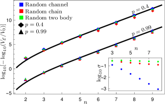
Figure 3: Volume contraction of the space of density matrices under a single realization of random, two-body, and chain FMs, together with the ansatz, eq. (14). Double-exponential contraction of the state space is shown. Inset: The standard deviation of the corresponding spectra (ignoring the ones). Self-averaging is observed only for the random general case, eq. (15).

In order to calculate the volume change due to the application of channel $\mathcal{E}$, we consider the manifold in which density matrices live. All density matrices can be expressed as $\openone/\mathop{\mathrm{Tr}}\nolimits\openone+\sum_{i=1}^{D}\alpha_{l}G_{l}$, where the $G_{l}$ form a traceless complete orthonormal set of matrices and $D=n^{d}-1$. Treating $\alpha$ as a real vector in $\mathbb{R}^{D}$, we can consider the volume (with the usual measure) in such $D=n^{d}-1$ space. For the qubit case this volume corresponds to the volume in the Bloch sphere representation. Consider now the hypercube defined by the points $\rho$ and $\rho+\epsilon G_{l}$, with $l=1,\dots,D$. The volume is $V_{0}=\epsilon^{D}$. Under the map, the hypercube will transform to the $D$-parallelotope defined by the corners $\mathcal{E}(\rho)$ and $\mathcal{E}(\rho+\epsilon G_{l})$ whose signed volume is $V_{\mathcal{E}}=V_{0}\det\mathcal{E}=V_{0}\prod_{l}\lambda_{l}$, where $\lambda_{l}$ are the eigenvalues of $\mathcal{E}$.

We calculate the volume contraction for several of the channels presented in this paper. First, consider the case of the random CG channel defined in eq. (15). Recall that the spectrum has an eigenvalue of 1 degenerated $C(d^{2}+n-1,n)$ times. We assume that the other eigenvalues are $p$, based on self-averaging and the spectral gap observed. This leads to a volume contraction given by

$$\frac{V_{\mathcal{E}}}{V_{0}}\approx p^{\left[d^{2n}-{\textstyle\begin{pmatrix}d^{2}+n-1\\ n\end{pmatrix}}\right]}.$$ (14)

Note that this is a double exponential in the number of particles. In fig. 3 we show a comparison between this approximation and a single realization of the channel for a varying number of qubits.

This implies that exploring the space of states, even with very efficient detectors, is extremely difficult. This is coherent with the difficulties found in quantum tomography [32, 33]. Fortunately, the fraction of the Hilbert space in which nature lives, seems to be much smaller [34, 35].

Due to Uhlmann’s theorem [36], fuzzy states are majorized by exact ones, i.e. $\mathcal{F}[\rho]\prec\rho$. This means that any convex function of the density matrices, such as the von Neumann entropy [37], a wide class of entanglement measures [38] and other quantum correlations [39], will decrease under FM.

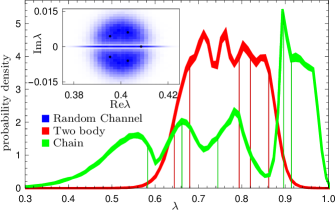
Figure 4: Probability density of the spectrum (aside from the 1s’) for random FM, two-body, and one-dimensional chains. The calculation is done for six qubits, $\gamma=\text{diag}\{5,1\}$, and $10^{5}$ realizations. For 2-body, and 1-d chains we divided the data into 10 groups to obtain a standard deviation, which is plotted as the thickness of the curves. An example of a spectrum for a single realization is included as darker dots (inset) or lines (figure).

V.4 Spectrum

We now examine some features of the spectrum of FM. In the spectrum we observe exactly $C(d^{2}+n-1,n)$ ones, one for each block, confirming what we obtained using the Perron-Frobenius theorem. We also note that changing the probability of error, while maintaining the relative probabilities of other permutations fixed, just rescales the spectrum since $\text{Spec}(p\openone+(1-p)\mathcal{F})=p+(1-p)\text{Spec}(\mathcal{F})$. It must also be noted that for general channels, the spectrum is complex. However, for channels involving only swaps [e.g. eq. (3) and eq. (4)] the spectrum is real as the operator is symmetric.

To conclude, we analyze the spectrum for generic situations (see also [40] and [41]). To do so, we define random measuring devices characterized by the channels

$$\mathcal{F}_{\text{ran}}[\rho]=p\rho+(1-p)\sum_{P\in\mathcal{S}}p_{P}P[\rho],$$ (15)

where $p$ describes the probability of doing the correct measurement and the $p_{P}$ values are chosen uniformly and normalized such that $\sum_{P\in\mathcal{S}}p_{P}=1$. Random two-body and one-dimensional FMs are similarly defined, via eq. (3) and eq. (4) respectively. For a random measuring device, $\mathcal{F}_{\text{ran}}$, aside from the 1s eigenvalues discussed above, we observe self-averaging of the eigenvalues around $1-p$, see fig. 4. This implies a spectral gap of approximately $p$. For random 2-body and 1-dimensional FM there is a richer structure and, if existent, selfaveraging is much slower, see fig. 4.

VI Conclusions

In this work we have addressed the theoretical characterization of quantum systems from imperfect measurements and provided a solid framework in the language of quantum channels to build fuzzy and coarse grained descriptions of them. The former not only is a critical step for the latter, but furnishes a quantum channel scheme to address particle-indexing experimental errors. Fuzzy maps do not reduce the size of the system, yet they diminish non-symmetric correlations with respect to the permutation group generated by the elements defining them. Coarse graining maps, on the other hand, combine contributions from every particle in the system into a reduced state, effectively lowering the number of particles and giving rise to coarser particles. In this paper, besides their general definitions, we explicitly construct maps corresponding to typical situations encountered in present state-of-the-art experiments in many-body physics, e.g., two-body errors and low resolution apparatuses.

In order to illustrate the use of the proposed maps we apply them to describe entanglement waves in a spin-$1/2$ $XX$-chain. As expected, in the portrayal obtained, the quantum correlations in the system are partially concealed, reflecting a decoherence-like effect due to the loss of information intrinsic to FMs and CG measurements. Such an outcome may be of relevance for some of the results reported in [22].

Though it is well known that in practice we cannot reconstruct the whole state of a many-body quantum system, our framework offers tools to compute the accessible state set in a wide number of scenarios. In the last part of the paper we have carefully studied the symmetries and spectra of the FM and CG channels, and identified the set of invariant states as the completely symmetric states. Remarkably, considering nonsymmetric states, we have shown that the volume of the accessible states contracts at a doubly exponential rate when fuzzy-like noise is present, signaling the fragility of quantum correlation under imperfect detection.

VII Acknowledgments

Conversations with F. de Melo, T. H. Seligman, J. D. Urbina, and A. Diaz-Ruelas are also acknowledged. Support by projects CONACyT 285754 and UNAM-PAPIIT IG100518 and IG101421 is also acknowledged.

Appendix A Connection between ket-bras in $\mathcal{B}_{\gamma}$

In this section we provide the connection between elements of the computational basis lying in the same invariant sector of $\mathcal{F}$. This result is needed to prove that sectors $\mathcal{B}_{\gamma}$ (set of bounded operators spanned by the elements of the computational basis with matrix eigenvalue $\gamma$; see text for further details) are irreducible in the generic case.

Theorem 1 (Connection of elements in $\mathcal{B}_{\gamma}$).

Let ${|\vec{x}\rangle\langle\vec{y}|},\ \ {|\vec{x}^{\prime}\rangle\langle\vec{y}^{\prime}|}\in\mathcal{B}_{\gamma}$ where ${|\vec{x}\rangle}$, ${|\vec{y}\rangle}$, ${|\vec{x}^{\prime}\rangle}$ and ${|\vec{y}^{\prime}\rangle}$ are elements of the computational basis, and $\mathcal{B}_{\gamma}$ is the support of $\mathcal{F}_{\gamma}$; then $\exists P\in\mathcal{S}$ such that

$${|\vec{x}^{\prime}\rangle\langle\vec{y}^{\prime}|}=P{|\vec{x}\rangle\langle\vec{y}|}P^{\dagger}.$$ (16)

Proof.

Let us show that every ${|\vec{x}\rangle\langle\vec{y}|}\in\mathcal{B}_{\gamma}$ can be written as a permutation of a reference ket-bra, i.e., ${|\vec{x}\rangle\langle\vec{y}|}=P[{|\vec{x}_{\text{r}}^{\gamma}\rangle\langle\vec{y}_{\text{r}}^{\gamma}|}]$, where the subscript “r” stands for reference. Let us now rewrite

$${|\vec{x}\rangle\langle\vec{y}|}={|x_{1}\rangle\langle y_{1}|}\otimes\dots\otimes{|x_{N}\rangle\langle y_{N}|}.$$ (17)

By definition, there will be $\gamma_{i,j}$ instances of the single particle operator $|i\rangle\langle j|$. One can then order the particles such that the $\gamma_{0,0}$ operators $|0\rangle\langle 0|$ are firsts, the $\gamma_{0,1}$ operators $|0\rangle\langle 1|$ are next, and so on, until the $\gamma_{d-1,d-1}$ operators $|d-1\rangle\langle d-1|$. This is the reference operator. In other words,

$${|\vec{x}_{\text{r}}^{\gamma}\rangle\langle\vec{y}_{\text{r}}^{\gamma}|}=|0\rangle\langle 0|^{\otimes\gamma_{0,0}}\otimes|0\rangle\langle 1|^{\otimes\gamma_{0,1}}\otimes\\ \dots\otimes|d-1\rangle\langle d-1|^{\otimes\gamma_{d-1,d-1}}.$$ (18)

Such a permutation will be called $P$. Let ${|\vec{x}^{\prime}\rangle\langle\vec{y}^{\prime}|}\in\mathcal{B}_{\gamma}$ be another element of the computational basis characterized by the same $\gamma$, and let $P^{\prime}$ be the corresponding permutation. Then, since

$${|\vec{x}\rangle\langle\vec{y}|} =P{|\vec{x}_{\text{r}}^{\gamma}\rangle\langle\vec{y}_{\text{r}}^{\gamma}|}P^{\dagger}$$ (19)

$${|\vec{x}^{\prime}\rangle\langle\vec{y}^{\prime}|} =P^{\prime}{|\vec{x}_{\text{r}}^{\gamma}\rangle\langle\vec{y}_{\text{r}}^{\gamma}|}P^{\prime\dagger},$$ (20)

we have that

$${|\vec{x}\rangle\langle\vec{y}|} =P(P^{\prime})^{\dagger}{|\vec{x}^{\prime}\rangle\langle\vec{y}^{\prime}|}P^{\prime}P^{\dagger}$$ (21)

$$=P^{\prime\prime}{|\vec{x}^{\prime}\rangle\langle\vec{y}^{\prime}|}(P^{\prime\prime})^{\dagger},$$ (22)

with $P^{\prime\prime}=P(P^{\prime})^{\dagger}$. This completes the proof. ∎

Appendix B Invariant states

In the text, using the symmetries of the generic fuzzy map and the Perron-Frobenius theorem, we have proven that a matrix $\Delta$ is invariant under generic FM if and only if it is invariant under any permutation. Here we give a theorem that holds only for Hermitian positive-definite operators, but that holds for nongeneric maps.

Theorem 2 (Invariant Hermitian matrices).

Let $\Delta$ be a bounded positive-definite operator, and $\mathcal{F}$ an FM defined by a probability vector $\vec{p}$ whose non-zero entries multiply terms corresponding to a set of permutations $\mathcal{A}$. Then,

$$P[\Delta]=\Delta\ \ \forall P\in\text{G}_{\mathcal{A}},$$ (23)

where $\text{G}_{\mathcal{A}}$ is the permutation group generated by $\mathcal{A}$.

Proof.

Note that if $\mathcal{F}[\Delta]=\Delta$, then $\mathop{\mathrm{Tr}}\nolimits[\Delta^{2}]=\mathop{\mathrm{Tr}}\nolimits\left[\mathcal{F}[\Delta]^{2}\right]$ holds. For density matrices this equality simply means that the purity is preserved. Developing the expression we get

$$\mathop{\mathrm{Tr}}\nolimits[\Delta^{2}] =\mathop{\mathrm{Tr}}\nolimits\left[\mathcal{F}[\Delta]^{2}\right]$$

$$=\mathop{\mathrm{Tr}}\nolimits\left[\left(\sum_{P\in\mathcal{A}}p_{P}P\Delta P^{\dagger}\right)^{2}\right]$$

$$=\sum_{P\in\mathcal{A}^{\prime}}q_{P}\mathop{\mathrm{Tr}}\nolimits\left[P\Delta P^{\dagger}{}\Delta\right],$$ (24)

where the $q_{P}$s are quadratic functions of the $p_{P}$s and $\mathcal{A}^{\prime}$ is a set of permutations generated by pairwise concatenations of elements in $\mathcal{A}$. Note that the $q_{P}$s form a probability distribution. This follows from the fact that each $q_{P}$ is a sum of elements of a product distribution (see the second inequality). Thus, the sum in eq. (24) is a convex combination of traces. Observe that $\mathcal{A}\subseteq\mathcal{A}^{\prime}$, where the equality holds only if $\mathcal{A}$ is a permutation group. Using the Bellman inequalities [42, 43] we have $\mathop{\mathrm{Tr}}\nolimits[P\Delta P^{\dagger}\Delta]\leq\mathop{\mathrm{Tr}}\nolimits[\Delta^{2}]$, hence the convex combination in eq. (24) equals $\mathop{\mathrm{Tr}}\nolimits\Delta^{2}$ only if $\mathop{\mathrm{Tr}}\nolimits[\Delta^{2}]=\mathop{\mathrm{Tr}}\nolimits[P\Delta P^{\dagger}{}\Delta]$.

Consider now the trace norm,

$$||\Delta-P{\Delta}P^{\dagger}||_{2}^{2} =\mathop{\mathrm{Tr}}\nolimits\left[\left|\Delta-P\Delta P^{\dagger}{}\right|^{2}\right]$$

$$=\mathop{\mathrm{Tr}}\nolimits\left[\left(\Delta-P\Delta P^{\dagger}{}\right)^{2}\right]$$

$$=\mathop{\mathrm{Tr}}\nolimits\left[\Delta^{2}-\Delta P\Delta P^{\dagger}{}-P\Delta P^{\dagger}{}\Delta\right.$$

$$\qquad\qquad\left.+P\Delta^{2}P^{\dagger}{}\right]$$

$$=2\left(\mathop{\mathrm{Tr}}\nolimits\left[\Delta^{2}\right]-\mathop{\mathrm{Tr}}\nolimits\left[P\Delta P^{\dagger}{}\Delta\right]\right)$$

$$=0.$$

The second equality follows from the Hermiticity of $\Delta$. Therefore, by the properties of norms, $\Delta=P\Delta P^{\dagger}$ for all $P\in\mathcal{A}^{\prime}$.

Note that if $\Delta$ is invariant under permutations in $\mathcal{A}^{\prime}$, then it is invariant under the permutation group generated by it, which in turn is the same group generated by $\mathcal{A}$, i.e., $\text{G}_{\mathcal{A}}$. ∎

References

- [1] John Archibald Wheeler and Wojciech H Zurek, editors. Quantum theory and measurement. Princeton University Press, Princeton, NJ, 1983.
- [2] Herwig Ott. Single atom detection in ultracold quantum gases: a review of current progress. Rep. Prog. Phys., 79(5):054401, 2016.
- [3] Dmitry A. Abanin, Ehud Altman, Immanuel Bloch, and Maksym Serbyn. Colloquium: Many-body localization, thermalization, and entanglement. Rev. Mod. Phys., 91:021001, 2019.
- [4] Immanuel Bloch. Quantum simulations come of age. Nat. Phys., 14:1159–1162, 2018.
- [5] Howard M Wiseman and Gerard J Milburn. Quantum Measurement and Control. Cambridge University Press, New York, 2010.
- [6] Kurt Jacobs. Quantum Measurement Theory and its Applications. Cambridge University Press, 2014.
- [7] H Häffner, W Hänsel, C F Roos, J Benhelm, D Chek-al kar, M Chwalla, T Körber, U D Rapol, M Riebe, P O Schmidt, C Becher, O Gühne, W Dür, and R Blatt. Scalable multiparticle entanglement of trapped ions. Nature, 438(7068):643–646, 2005.
- [8] John Preskill. Quantum Computing in the NISQ era and beyond. Quantum, 2:79, 2018.
- [9] A. Peres. Quantum Theory: Concepts and Methods. Fundamental Theories of Physics. Springer Netherlands, 1995.
- [10] M. B. Mensky. Quantum restrictions for continuous observation of an oscillator. Phys. Rev. D, 20:384–387, 1979.
- [11] Stan Gudder. Non-disturbance for fuzzy quantum measurements. Fuzzy Sets and Systems, 155(1):18 – 25, 2005.
- [12] Claudio Carmeli, Teiko Heinonen, and alessandro toigo. Why unsharp observables? Int. J. Theo. Phys., 47(1):81–89, 2008.
- [13] Paul Busch and Gregg Jaeger. Unsharp quantum reality. Found. Phys., 40(9):1341–1367, 2010.
- [14] Johannes Kofler and Časlav Brukner. Classical world arising out of quantum physics under the restriction of coarse-grained measurements. Phys. Rev. Lett., 99:180403, 2007.
- [15] Johannes Kofler and Časlav Brukner. Conditions for quantum violation of macroscopic realism. Phys. Rev. Lett., 101:090403, 2008.
- [16] Cristhiano Duarte, Gabriel Dias Carvalho, Nadja K. Bernardes, and Fernando de Melo. Emerging dynamics arising from coarse-grained quantum systems. Phys. Rev. A, 96:032113, 2017.
- [17] Pedro Silva Correia and Fernando de Melo. Spin-entanglement wave in a coarse-grained optical lattice. Phys. Rev. A, 100:022334, 2019.
- [18] Gabriel Dias Carvalho and Pedro Silva Correia. Decay of quantumness in a measurement process: Action of a coarse-graining channel. Phys. Rev. A, 102:032217, 2020.
- [19] Consider to be a set of observables tomographically complete, suffering from the fuzzy noise. Then the measurable averages are for all . Since are the components of in the complete operator basis , then is the state accessible tomographically.
- [20] Takeshi Fukuhara, Adrian Kantian, Manuel Endres, Marc Cheneau, Peter Schauß, Sebastian Hild, David Bellem, Ulrich Schollwöck, Thierry Giamarchi, Christian Gross, Immanuel Bloch, and Stefan Kuhr. Quantum dynamics of a mobile spin impurity. Nat. Phys., 9:235–241, 2013.
- [21] Takeshi Fukuhara, Sebastian Hild, Johannes Zeiher, Peter Schauß, Immanuel Bloch, Manuel Endres, and Christian Gross. Spatially resolved detection of a spin-entanglement wave in a bose-hubbard chain. Phys. Rev. Lett., 115:035302, 2015.
- [22] Jacob F Sherson, Christof Weitenberg, Manuel Endres, Marc Cheneau, Immanuel Bloch, and Stefan Kuhr. Single-atom-resolved fluorescence imaging of an atomic Mott insulator. Nature, 467(7311):68–72, 2010.
- [23] W S Bakr, A Peng, M E Tai, R Ma, J Simon, and 2010. Probing the superfluid–to–Mott insulator transition at the single-atom level. Science, 239:547–550, 2010.
- [24] V Subrahmanyam. Entanglement dynamics and quantum-state transport in spin chains. Phys. Rev. A, 69(3):034304, 2004.
- [25] Luigi Amico, Andreas Osterloh, Francesco Plastina, Rosario Fazio, and G. Massimo Palma. Dynamics of entanglement in one-dimensional spin systems. Phys. Rev. A, 69:022304, 2004.
- [26] Norio Konno. Limit theorem for continuous-time quantum walk on the line. Phys. Rev. E, 72:026113, 2005.
- [27] Leonardo Mazza, Davide Rossini, Rosario Fazio, and Manuel Endres. Detecting two-site spin-entanglement in many-body systems with local particle-number fluctuations. New J. Phys, 17(1):013015, 2015.
- [28] W Feller. An Introduction to Probability Theory and its Applications, volume 1. John Wiley and Sons, Inc., 1968.
- [29] Carl D. Meyer. Matrix Analysis and Applied Linear Algebra. Society for Industrial and Applied Mathematics, 2001.
- [30] Barry Simon. Real Analysis. American Mathematical Society, Providence, Rhode Island, 2015.
- [31] D Burgarth, G Chiribella, V Giovannetti, P Perinotti, and K Yuasa. Ergodic and mixing quantum channels in finite dimensions. New J. Phys., 15(7):073045, 2013.
- [32] K. Banaszek, M. Cramer, and D. Gross. Focus on quantum tomography. New J. Phys, 15(12):125020, 2013.
- [33] Steven T Flammia, David Gross, Yi-Kai Liu, and Jens Eisert. Quantum tomography via compressed sensing: error bounds, sample complexity and efficient estimators. New J. Phys., 14(9):095022, 2012.
- [34] Román Orús. Tensor networks for complex quantum systems. Nature Reviews Physics, 1(9):538–550, 2019.
- [35] Carlos Pineda, Thomas Barthel, and Jens Eisert. Unitary circuits for strongly correlated fermions. Phys. Rev. A, 81(5):050303(R), 2010.
- [36] A. Uhlmann. The “transition probability” in the state space of a -algebra. Rep. Math. Phys., 9(2):273 – 279, 1976.
- [37] Ingemar Bengtsson and Karol Zyczkowski. Geometry of Quantum States: An Introduction to Quantum Entanglement. Cambridge University Press, 2006.
- [38] R. Horodecki, P. Horodecki, M. Horodecki, and K. Horodecki. Quantum entanglement. Rev. Mod. Phys., 81(2):865–942, 2009.
- [39] Asutosh Kumar. Conditions for monogamy of quantum correlations in multipartite systems. Phys. Lett. A, 380(38):3044 – 3050, 2016.
- [40] Wojciech Bruzda, Valerio Cappellini, Hans-Jürgen Sommers, and Karol Życzkowski. Random quantum operations. Phys. Lett. A, 373(3):320 – 324, 2009.
- [41] Lucas Sá, Pedro Ribeiro, and Tomaž Prosen. Spectral and steady-state properties of random liouvillians. J. Phys. A, 53(30):305303, 2020.
- [42] Richard Bellman. Some Inequalities for Positive Definite Matrices, pages 89–90. Birkhäuser Basel, Basel, 1980.
- [43] Houqing Zhou. On some trace inequalities for positive definite Hermitian matrices. J Inequal Appl, 2014(1):64, 2014.