Sandslash: A Two-Level Framework for Efficient Graph Pattern Mining

Abstract.

Graph pattern mining (GPM) is used in diverse application areas including social network analysis, bioinformatics, and chemical engineering. Existing GPM frameworks either provide high-level interfaces for productivity at the cost of expressiveness or provide low-level interfaces that can express a wide variety of GPM algorithms at the cost of increased programming complexity. Moreover, existing systems lack the flexibility to explore combinations of optimizations to achieve performance competitive with hand-optimized applications.

We present Sandslash, an in-memory Graph Pattern Mining (GPM) framework that uses a novel programming interface to support productive, expressive, and efficient GPM on large graphs. Sandslash provides a high-level API that needs only a specification of the GPM problem, and it implements fast subgraph enumeration, provides efficient data structures, and applies high-level optimizations automatically. To achieve performance competitive with expert-optimized implementations, Sandslash also provides a low-level API that allows users to express algorithm-specific optimizations. This enables Sandslash to support both high-productivity and high-efficiency without losing expressiveness. We evaluate Sandslash on shared-memory machines using five GPM applications and a wide range of large real-world graphs. Experimental results demonstrate that applications written using Sandslash high-level or low-level API outperform that in state-of-the-art GPM systems AutoMine, Pangolin, and Peregrine on average by 13.8$\times$, 7.9$\times$, and 5.4$\times$, respectively. We also show that these Sandslash applications outperform expert-optimized GPM implementations by 2.3$\times$ on average with less programming effort.

1. Introduction

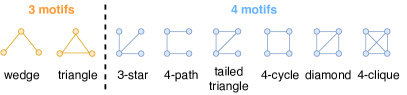
Graph pattern mining (GPM) problems arise in many application domains (chemical, ; Motif, ; Protein, ; Social, ). One example is motif counting (Motifs2, ; Motif3, ; Breaking, ), which counts the number of occurrences of certain structural patterns, such as those shown in Fig. 1, in a given graph. These numbers are often different for graphs from different domains, so they can be used as a “signature” to infer, for example, the probable origin of a graph (Social, ).

Programming efficient parallel solutions for GPM problems is challenging. Most problems are solved by searching the input graph for patterns of interest. For efficiency, the search space needs to be pruned aggressively without compromising correctness, but this can be complicated since the pruning strategy usually depends on the structural patterns of interest. Complicated book-keeping data structures are needed to avoid repeating work during the search process; maintaining these data structures efficiently in a parallel program can be challenging. A number of GPM frameworks have been proposed to reduce the burden on the programmer (Arabesque, ; RStream, ; Kaleido, ; AutoMine, ; Pangolin, ; Peregrine, ; GraphZero, ). They can be categorized into high-level and low-level systems: they both simplify GPM programming compared to hand-optimized code, but they make different tradeoffs and have different limitations.

High-level systems such as AutoMine (AutoMine, ) and Peregrine (Peregrine, ) take specifications of patterns as input and leverage static analysis techniques to automatically generate GPM programs for those patterns. These systems promote productivity, but they may not allow expressing more efficient algorithms. Low-level systems such as RStream (RStream, ) and Pangolin (Pangolin, ) provide low-level API functions for the user to control the details of mining process, and they can be used to implement solutions for a wider variety of GPM problems but they require more programming effort. Moreover, both high-level and low-level systems lack the ability to explore combinations of optimizations that have been implemented in handwritten GPM solutions for different problems. Therefore, they do not match the performance of hand-optimized solutions.

Figure 1. 3-vertex (left) and 4-vertex (right) motifs.

In this paper, we present Sandslash, an in-memory GPM system that provides high productivity and efficiency without compromising generality. Sandslash provides a novel programming interface that separates problem specifications from algorithmic optimizations. The Sandslash high-level interface requires the user to provide only the specification of the pattern(s) of interest. Sandslash analyzes the specification and automatically enables efficient search strategies, data representations, and optimizations. To customize the GPM algorithm and improve performance further, the user can leverage the Sandslash low-level interface to exploit application-specific knowledge. This two-level API combines the expressiveness of existing low-level systems while achieving the productivity enabled by existing high-level systems. Meanwhile, Sandslash automates a number of optimizations that have been used previously only in handwritten solutions to particular GPM problems. Since these optimizations are missing in previous high-level systems, Sandslash can outperform these systems in most cases. In addition, low-level Sandslash exposes fine-grained control to allow the user to compose low-level optimizations, which leads to better performance than hand-optimized implementations without requiring the programmer to code the entire solution manually.

Evaluation on a 56-core CPU demonstrates that applications written using Sandslash high-level API outperform the state-of-the-art GPM systems, AutoMine (AutoMine, ), Pangolin (Pangolin, ), and Peregrine (Peregrine, ) by 7.7$\times$, 6.2$\times$ and 3.9$\times$ on average, respectively. Applications using Sandslash low-level API outperform AutoMine, Pangolin, and Peregrine by 22.6$\times$, 27.5$\times$ and 7.4$\times$ on average, respectively. Sandslash applications are also 2.3$\times$ faster on average than expert-optimized GPM applications.

This work makes the following contributions:

• We present Sandslash, an in-memory GPM system that supports productive, expressive, and efficient pattern mining on large graphs.

• We propose a high-level programming model in which the choice of efficient search strategies, subgraph data structures, and high-level optimizations are automated, and we expose a low-level programming model to allow the programmers to express algorithm-specific optimizations.

• We holistically analyze the optimization techniques available in hand-tuned applications and separately enabled them in the two levels. We show that existing optimizations in the literature applied to specific problems/applications can be applied more generally to other GPM problems. The user is allowed to flexibly control and explore the combination of optimizations.

• Experimental results show that Sandslash substantially outperforms existing GPM systems. They also show the impact of (and the need for) Sandslash’s low-level API. Compared to expert-optimized applications, Sandslash achieves competitive performance with less programming effort.

2. Problem Definition

We use standard definitions in graph theory for subgraph, vertex-induced and edge-induced subgraphs, isomorphism and automorphism (definitions in Appendix B.7). Isomorphic graphs $G_{1}$ and $G_{2}$ are denoted as $G_{1}\simeq G_{2}$. If $G_{1}$ and $G_{2}$ are automorphic, they are denoted as $G_{1}\cong G_{2}$.

A pattern is a graph defined explicitly or implicitly. An explicit definition specifies the vertices and edges of the graph while an implicit definition specifies its desired properties. Given a graph $G$ and a pattern $\mathcal{P}$, an embedding $X$ of $\mathcal{P}$ in $G$ is a vertex- or edge-induced subgraph of $G$ s.t. $X\simeq\mathcal{P}$. In this work, we focus on connected subgraphs and patterns only.

Given a graph $G$ and a set of patterns $S_{p}=\{\mathcal{P}_{1},\dots,\mathcal{P}_{n}\}$, GPM finds all the vertex- or edge-induced embeddings of $\mathcal{P}_{i}$ in $G$. For explicit-pattern problems, the solver finds embeddings of the given pattern(s). For implicit-pattern problems, $S_{p}$ is not explicitly given but described using some rules. Therefore, the solver must find the patterns as well as the embeddings. If the cardinality of $S_{p}$ is 1, we call this problem a single-pattern problem. Otherwise, it is a multi-pattern problem. Note that graph pattern matching (GPMatch, ) finds embeddings only for explicit pattern(s), whereas graph pattern mining (GPM, ) solves both explicit- and implicit-pattern problems.

In some GPM problems, the required output is the listing of embeddings. However, in other GPM problems, the user wants to get statistics such as a count of the occurrences of the pattern(s) in $G$. The particular statistic for $\mathcal{P}$ in $G$ is termed its support. The support has the anti-monotonic property if the support of a supergraph does not exceed the support of a subgraph. Counting and listing may have different search spaces because listing requires enumerating every embedding while counting does not.

Figure 2. A portion of a vertex-induced subgraph tree with 3 levels. Lightly colored subgraphs are removed from consideration by automorphism checks.

Graph Pattern Mining Problems

We consider five GPM problems in a given input graph $G$.

(1) Triangle Counting (TC): The problem is to count the number of triangles in $G$. It uses vertex-induced subgraphs.

(2) $k$-Clique Listing ($k$-CL): A subset of vertices $W$ of $G$ is a clique if every pair of vertices in $W$ is connected by an edge in $G$. If the cardinality of $W$ is $k$, this is called a $k$-clique (triangles are 3-cliques). The problem of listing $k$-cliques is denoted $k$-CL, and it uses vertex-induced subgraphs.

(3) Subgraph Listing (SL): The problem is to enumerate all edge-induced subgraphs of $G$ isomorphic to a pattern $\mathcal{P}$.

(4) $k$-Motif Counting ($k$-MC): This problem counts the number of occurrences of the different patterns that are possible with $k$ vertices. In the literature, each pattern is called a motif or graphlet. Fig. 1 shows all 3-motifs and 4-motifs. This problem uses vertex-induced subgraphs.

(5) $k$-Frequent Subgraph Mining ($k$-FSM): Given integer $k$ and a threshold $\sigma_{min}$ for support, $k$-FSM finds patterns with $k$ or fewer edges and lists a pattern $\mathcal{P}$ if its support is greater than $\sigma_{min}$. This is called a frequent pattern. If $k$ is not specified, it is set to $\infty$, meaning it considers all possible values of $k$. This problem finds edge-induced subgraphs.

2.1. Subgraph Tree and Vertex/Edge Extension

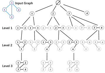
The subgraph tree is a useful abstraction for organizing GPM computations. The vertex-induced subgraphs of a given input graph $G{=}(V,E)$ can be ordered naturally by containment (i.e., if one is a subgraph of the other). It is useful to represent this partial order as a vertex-induced subgraph tree whose vertices represent the subgraphs. Level $l$ of the tree represents subgraphs with $l+1$ vertices. The root vertex of the tree represents the empty subgraph. Intuitively, subgraph $S_{2}{=}(W_{2},E_{2})$ is a child of subgraph $S_{1}{=}(W_{1},E_{1})$ in this tree if $S_{2}$ can be obtained by extending $S_{1}$ with a single vertex $v\notin W_{1}$ that is connected to some vertex in $W_{1}$ ($v$ is in the neighborhood of subgraph $S_{1}$); this process is called vertex extension. Formally, this can be expressed as $W_{2}{=}W_{1}\cup\{v\}$ where $v\notin W_{1}$ and there is an edge $(v,u)\in E$ for some $u\in W_{1}$. It is useful to think of the edge connecting $S_{1}$ and $S_{2}$ in the tree as being labeled by $v$. Fig. 2 shows a portion of a vertex-induced subgraph tree with three levels (for lack of space, not all subgraphs are shown). Note that a given subgraph can occur in multiple places in this tree. For example, in Fig. 2, the subgraph containing vertices 1 and 2 occurs in two places. These identical subgraphs are automorphisms (automorphic with each other).

The edge-induced subgraph tree for a given input graph can be defined in a similar way. Edge extension extends an edge-induced subgraph $S_{1}$ with a single edge $(u,v)$ provided at least one of the endpoints of the edge is in $S_{1}$.

The subgraph tree is a property of the input graph. When solving a specific GPM problem, a solver uses the subgraph tree as a search tree and builds a prefix of the subgraph tree that depends on the problem, pattern, and other aspects of the implementation (e.g., if the size of the pattern is $k$, subgraphs of larger size are not explored). We use the term embedding tree to refer to the prefix of the subgraph tree that has been explored at any point in the search.

Finally, since a pattern is a graph, its connected subgraphs form a tree as well. These subgraphs are called sub-patterns, and the tree formed by them is called the sub-pattern tree.

Figure 3. Overview of Sandslash. Dash indicates optional.

3. Sandslash API

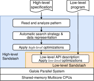
Fig. 3 shows the overview of Sandslash, which is built on top of the Galois (Galois, ) parallel system. In this section, we describe the high-level and low-level API of Sandslash.

3.1. High-Level API

Table 1 shows Sandslash high-level API that can be used to specify a GPM problem (as defined in Section 2). The first two required flags define whether the embeddings are vertex-induced or edge-induced and whether the matched embeddings need to be listed or counted. The third required flag defines if the set of patterns is explicit or implicit. If they are explicit, then the patterns must be defined using getExplicitPatterns(). Otherwise, the rule to select implicit patterns must be defined using isImplicitPattern(). process() is a function for customized output. terminate() specifies an optional early termination condition (useful to implement pattern existence query). The default support for each pattern in Sandslash is count (number of embeddings). The support can be customized using three functions: getSupport() defines the support of an embedding, isSupportAntiMonotonic() defines if the support has the anti-monotonic property, and reduce() defines the reduction operator (e.g., sum) for combining the support of different embeddings of the same pattern. In addition, Sandslash has a runtime parameter $k$ to denote the maximum size (vertices or edges) of the (vertex- or edge-induced) embeddings to find.

Flag	Required	Example: spec for FSM
isVertexInduced	yes	false
isListing	yes	false
isExplicit	yes	false
Function	Required	Example: user code for FSM
getExplicitPatterns()	no	-
isImplicitPattern(Pattern pt)	no	pt.support $\geq$ MIN_SUPPORT
process(Embedding emb)	no	-
terminate(Embedding emb)	no	-
isSupportAntiMonotonic()	no	true
getSupport(Embedding emb)	no	getDomainSupport(emb)
reduce(Support s1, Support s2)	no	mergeDomainSupport(s1, s2)

Table 1. Left column lists Sandslash high-level API flags and functions. Right column is the spec and user code of FSM using the API.

The problem specifications for TC, CL, SL, and MC are straightforward. All four specify an explicit set of patterns. Each pattern is specified using an edge-list. For example, in TC, the user provides an edge-list of {(0,1) (0,2) (1,2)}. Table 1’s right column shows the problem specification for FSM. isImplicitPattern() is used to specify that only frequent patterns (i.e., those with support greater than MIN_SUPPORT) are of interest. FSM uses the domain (MNI) support, which is anti-monotonic, and its associated reduce operation.

3.2. Low-Level API

⬇

1bool toExtend(Embedding emb, Vertex v);

2bool toAdd(Embedding emb, Vertex u);

3bool toAdd(Embedding emb, Edge e);

4Pattern getPattern(Embedding emb);

5void localReduce(int depth, vector<Support> &supports);

6void initLG(Graph gg, Vertex v, Graph lg);

7void initLG(Graph gg, Edge e, Graph lg);

8void updateLG(Graph lg);

Listing 1: Sandslash low-level API functions.

Sandslash low-level API is shown in LABEL:lst:lo-api. Since the mining process includes search, extension, and reduction, control of the mining process includes customizing (1) the graph to search (initLG and updateLG), (2) the extension candidates and their selection (toAdd and toExtend), and (3) the reduction operations to perform (getPattern and localReduce). Sandslash low-level API exposes necessary control and is expressive enough to support sophisticated algorithms.

toExtend determines if a vertex $v$ in embedding $emb$ must be extended. toAdd decides if extending embedding $emb$ with vertex $u$ (or edge $e$) is allowed. toExtend and toAdd do fine-grained pruning to reduce search space (Appendix B.4).

getPattern() returns the pattern of an embedding. This function can be used to replace the default graph isomorphism test with a custom method to identify patterns (Appendix B.5). Note that Pattern can be user-defined; therefore, Sandslash can support custom aggregation-keys like Fractal (Fractal, ).

Some algorithms (PGD, ) do local counting for each vertex or edge instead of global counting. Sandslash provides localReduce to support local counting. Listings LABEL:lst:motif-opt and LABEL:lst:4motif-lc in the Appendix show 3-MC and 4-MC using this low-level API.

Some algorithms (KClique, ) search local (sub-)graphs instead of the (global) input graph. initLG and updateLG can be used to support search on local graphs. LABEL:lst:kcl-opt in the Appendix shows optimized $k$-CL using the Sandslash low-level API.

3.3. Productivity and Expressiveness

	Language	TC	$k$-CL	SL	$k$-MC	$k$-FSM
Hand	C/C++	GAP (GAPBS, )	KClist (KClique, )	CECI (CECI, )	PGD (PGD, )	DistGraph (DistGraph, )
Optimized		89	394	3,000	2,538	17,459
Arabesque (Arabesque, )	Java	43	31	-	35	80
RStream (RStream, )	C++	101	61	-	98	125
Fractal (Fractal, )	Java/Scala	6	6	5	12	48
Pangolin (Pangolin, )	C++	26	36	57	82	252
AutoMine (AutoMine, )	C++	0	0	N/S	-	N/S
Peregrine (Peregrine, )	C++	0	0	0	54	68
Sandslash-Hi	C++	0	0	0	9	75
Sandslash-Lo	C++	-	67	-	61	-

Table 2. Lines of code in Sandslash, other GPM systems, and expert-optimized GPM applications. N/S: not supported; ‘-’: supported but not yet implemented. AutoMine, Peregrine are high-level systems, Sandslash is a two-level system, and the rest are low-level systems.

Table 2 compares the lines of code of GPM applications in Sandslash and other GPM systems with that of hand-optimized GPM applications. Sandslash’s high-level specification requires similar programming effort to that of other high-level systems. Zero lines of C++ user code are needed for explicit pattern problems (only flags and pattern edgelist are required). Sandslash’s low-level programs require only a little more programming effort since all high-level optimizations are automatically performed by the system. Note that Fractal is classified as a low-level system because it supports high-level API only for single, explicit-pattern problems (i.e., SL). For implicit-pattern problems like FSM, Fractal requires the user to write code for iterative expand-aggregate-filter.

As for expressiveness, since Sandslash uses the vertex/edge extension model that existing low-level systems use, it is as expressive as these systems. Sandslash high-level API is adequate for the specification of GPM problems implemented in previous GPM systems and is easily extendable to support new features (e.g., anti-edges and anti-vertices in Peregrine) that fit in the vertex/edge extension abstraction. In contrast, existing high-level systems use a pattern-aware model based on set intersection and set difference which does not work well for implicit-pattern problems. For example, FSM implemented in Peregrine and AutoMine (details in Appendix  B.3) needs to enumerate possible patterns before the search, which causes non-trivial performance overhead. In Section 4, we show that the vertex/edge extension model can be effectively augmented with pattern awareness, and more importantly, together with the high-level optimizations, Sandslash can even outperform existing high-level systems, with the same productivity.

All existing GPM systems lack support for some of the functions in Sandslash low-level API. Consequently, they either lack such optimizations or expose an even lower-level API to give the user full control of the mining process at the cost of preventing the system from applying high-level optimizations. For example, Fractal (Fractal, ) allows the user to compose low-level optimizations using custom subgraph enumerators. In contrast, Sandslash low-level API is designed to enable the user to express custom algorithms while allowing the system to apply high-level optimizations and explore different traversal orders. For example, to implement local graph search in Sandslash, the user only implements initialization/modification functions for the local graph, which allows Sandslash to apply all possible high-level optimizations in Table 3(a) during exploration. In Fractal, the user must change the entire exploration which includes implementing all the optimizations by hand; the system cannot apply optimizations automatically. This also applies for other low-level optimizations like local counting.

4. High-Level Sandslash

This section describes high-level Sandslash. It uses efficient search strategies (Section 4.1), data representations (Section 4.2), and high-level optimizations (Section 4.3).

4.1. Search Strategies

Given a pattern $\mathcal{P}$ with $k$ vertices, we can build the subgraph tree described in Section 2 to a depth $k$ and test each subgraph $X$ at the leaf of the tree to see if $X\simeq\mathcal{P}$. This approach is pattern-oblivious and works effectively for any pattern (even if $\mathcal{P}$ is implicit). In Sandslash, we augment this model with pattern-awareness. If the user defines an explicit pattern problem, Sandslash does pattern analysis and constructs a matching order (Appendix B.3) to guide vertex extension. This prunes the search tree and avoids isomorphism tests. As the same subgraph (i.e., automorphisms) may occur in multiple places of the tree, Sandslash uses the standard symmetry breaking technique (see Appendix B.1) to avoid over-counting.

GPM solutions must also decide the order in which the subgraph tree is explored. Any top-down visit order on the tree can be used. Breadth-first search (BFS) exposes more parallelism while requiring more storage than a depth-first search (DFS). DFS consumes less memory but has fewer opportunities for parallel execution. Arabesque, RStream, and Pangolin use BFS exploration while the other GPM systems in Table 2 use DFS exploration. Sandslash performs a pseudo-DFS parallel exploration (following convention this area, we refer to it simply as DFS), using the following strategy.

• Each vertex $v$ in the input graph corresponds to a vertex-induced subgraph for the vertex set $\{v\}$ and therefore corresponds to a search tree vertex $t_{v}$.

• The subtree below each such tree vertex $t_{v}$ is explored in DFS order. This is a task executed serially by a single thread. When the exploration reaches the pattern size $k$, the support is updated appropriately.

• Multiple threads execute different tasks in parallel. The runtime uses work-stealing for thread load-balancing; the unit of work-stealing is a task.

Pattern filtering for implicit-pattern problems that use anti-monotonic support:

The search strategy described above mines implicit-pattern problems like FSM by enumerating all embeddings, binning them according to their patterns, and checking the support for each pattern. This can be optimized by exploiting the sub-pattern tree when the support is anti-monotonic (Section 2). If a sub-pattern does not have enough support, then its descendants in the sub-pattern tree will not have enough support and can be ignored due to the anti-monotonic property. Instead of pruning sub-patterns during post-processing, one can prune after generating all the embeddings for a given sub-pattern. This allows Sandslash to avoid generating the embeddings for descendant sub-patterns. This is easy in BFS since it generates embeddings level by level, and in each level, the entire list of the embeddings is scanned to aggregate support for each sub-pattern. However, this does not work for DFS of the sub-graph tree as DFS is done by each thread independently.

To handle pattern-wise aggregation, Sandslash performs a DFS traversal on the sub-pattern tree instead of the sub-graph tree. This ensures that the embeddings for a given sub-pattern are generated by a single thread using the same approach for pattern extension in hand-optimized gSpan (gSpan, ); i.e., the embeddings are gathered to their pattern bins during extension and canonicality is checked for each sub-pattern to avoid duplicate pattern enumeration. When the thread finishes extension in each level, the support for each sub-pattern can be computed using its own bin of embeddings.

4.2. Representation of Tree

Since subgraphs are created incrementally by vertex or edge extension of parent subgraphs in the embedding tree, the representation of subgraphs should allow structure sharing between parent and child subgraphs. We describe the information stored in the embedding tree and the concrete representation of the tree for vertex-induced sub-graphs first.

Figure 4. Embedding data structure (vertex-induced).

• Each non-root vertex in the tree points to its parent vertex.

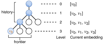
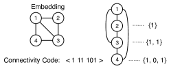
• Each non-root vertex in the tree corresponds to a subgraph obtained from its parent subgraph by vertex extension with some vertex $v$ of the input graph. The vertex set of a subgraph can be obtained by walking up the tree and collecting the vertices stored on the path to the root. These vertices are the predecessors of $v$ in the embedding; they correspond to vertices discovered before $v$ in that embedding. As shown in Fig. 4, the leaf containing $v_{3}$ represents the subgraph with a vertex set of $\{v_{3},v_{2},v_{1},v_{0}\}$, which are the vertices stored on the path to the root from this leaf.

• Given a set of vertices $W=\{v_{0},v_{1},\dots,v_{n}\}$ in a subgraph, the edges among them are obtained from the input graph $G$. To avoid repetitive look-ups, edge information is cached in the embedding tree. When performing vertex extension by adding a vertex $u$, the edges between $u$ and its predecessors in the embedding tree are determined and stored in the tree together with $u$. This set of edges can be represented compactly using a bit-vector of length $l$ for vertices at level $l$ of the tree. We call this bit-vector the connectivity code (see an example in Appendix B.6). This technique is called Memoization of Embedding Connectivity (MEC) (Pangolin, ).

• For edge-induced extension, a set of edges instead of vertices is stored for each embedding. There is no need to store connectivity for embeddings since the set of edges already contains this information.

• For a sub-pattern tree, embeddings of each sub-pattern are gathered as an embedding list (bin of embeddings). The search tree is constructed with sub-patterns as vertices, and each sub-pattern in the tree has an embedding list associated with it. Embedding connectivity is not needed as the sub-pattern contains this information.

4.3. High Level Optimizations

Sandslash automatically performs high-level optimizations without guidance from the user. Table 3(a) (left) lists which of these optimizations are applied to each application. Table 3(b) (left) lists which of them are supported by other GPM systems.

	High-level					Low-level
	SB	DAG	MO	DF	MNC	FP	CP	LG	LC
TC	✓	✓		✓
$k$-CL	✓	✓	✓	✓	✓			✓
SL	✓		✓	✓	✓
$k$-MC	✓			✓	✓	✓	✓		✓
$k$-FSM	✓			✓

(a) Optimizations applied to GPM applications.

			High-level					Low-level
	SB	DAG	MO	DF	MNC	FP	CP	LG	LC
AutoMine (AutoMine, )			✓		$\circledcirc$
Pangolin (Pangolin, )	✓	✓	✓			✓	✓
Peregrine (Peregrine, )	✓		✓		$\circledcirc$
Sandslash-Hi	✓	✓	✓	✓	✓
Sandslash-Lo	✓	✓	✓	✓	✓	✓	✓	✓	✓

(b) Optimizations supported by GPM frameworks. $\checkmark$: full support; $\circledcirc$: limited support.

Table 3. Optimizations enabled in Sandslash. High level optimizations: SB: Symmetry breaking; DF: Degree Filtering; DAG: orientation; MO: Matching Order; MNC: Memoization of Neighborhood Connectivity. Low-level optimizations: FP: Fine-grained Pruning; CP: Customized Pattern classification; LG: search on Local Graph; LC: Local Counting.

Symmetry Breaking (SB), Orientation (DAG), and Matching Order (MO): These optimizations are supported by at least one previous GPM system (Table 3(b)), so we describe them in Appendices B.1, B.2, and B.3. Sandslash applies SB for all GPM problems. Sandslash enables DAG only if it is a single explicit-pattern problem and if the pattern is a clique. It enables MO for single explicit-pattern problems except if the pattern is a triangle (because it is not beneficial).

Degree Filtering (DF): When searching for a pattern in which the smallest vertex degree is $d$, it is unnecessary to consider vertices with degree less than $d$ during vertex extension. When MO is enabled, at each level, only one vertex $v$ of the pattern is searched for, so all vertices with degree less than that of $v$ can also be filtered. This optimization (DF) has been used in a hand-optimized SL implementation, PSgL (PSgL, ). Sandslash enables DF for all GPM problems. DF is mostly beneficial for SL and $k$-CL with large values of $k$.

Figure 5. An example of connectivity memoization. ❶, ❷ and ❸ are timestamps to show the order of actions.

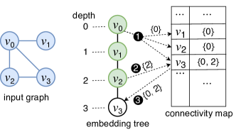
Memoizing of Neighborhood Connectivity (MNC): When extending an embedding $X=\{v_{0},\dots v_{n}\}$ by adding a vertex $u$, a common operation is to check the connectivity between $u$ and each vertex in $X$. To avoid repeated lookups in the input graph, we memoize connectivity information in a map (namely connectivity map) during embedding construction. The map takes a vertex ID (say $v$) and returns the positions in the embedding of the vertices connected to $v$. In Fig. 5, $v_{3}$ is connected to $v_{0}$ and $v_{2}$, so when $v_{3}$ is looked up in the map, the map returns 0 and 2, the embedding positions of $v_{0}$ and $v_{2}$. This map is generated incrementally during the construction of the embedding tree. Whenever a new vertex ($w$) is added to the current embedding, the map for the neighbors of $w$ that are not already in that embedding are updated with the position of $w$ in the embedding; when backing out of this step in the DFS walk, this information is removed from the map.

Fig. 5 shows how the connectivity map is updated during vertex extension. At time ❶, depth of $v_{0}$ is sent to the map to update the entries of $v_{1}$, $v_{2}$ and $v_{3}$ since $v_{1}$, $v_{2}$ and $v_{3}$ are neighbors of $v_{0}$ and they are not in the current embedding. At time ❷, depth of $v_{2}$ is sent to the map, and the entry of $v_{3}$ is updated. Note that although $v_{0}$ is also a neighbor of $v_{2}$, there is no need to update the entry of $v_{0}$ since $v_{0}$ already exists in the current embedding. When $v_{3}$ is added to the embedding, the map performs look up with $v_{3}$, and the positions {0, 2} are returned at time ❸. Therefore, we know that $v_{3}$ is connected to the 0-th and 2-th vertices in the embedding, which are $v_{0}$ and $v_{2}$. For parallel execution, the map is thread private, and each entry is represented by a bit-vector.

This optimization (MNC) has been used in a hand-optimized $k$-CL implementation, kClist (KClique, ), and a hand-optimized $k$-MC implementation, PGD (PGD, ). Sandslash enables this optimization for implicit-pattern problems that require vertex-induced embeddings and for explicit-pattern problems unless the pattern is a triangle; for triangles, Sandslash uses set intersection instead of MNC. In particular, Sandslash enables MNC for SL, an optimization that is missing in hand-optimized SL implementations (PSgL, ; CECI, ).

MNC does not exist in previous GPM systems such as Peregrine and AutoMine which use set intersection/differences to compute connectivity. Note that MNC is different from the vertex set buffering (VSB) technique used in Peregrine and AutoMine. To remove redundant computation, VSB buffers the vertex sets computed for a given embedding. However, for multi-pattern problems, different patterns may require buffering different vertex sets. Peregrine’s solution is to match one pattern at a time, which is inefficient for a large number of patterns. AutoMine’s solution is to only buffer one vertex set, which leads to recomputing unbuffered vertex sets. The other alternative is to buffer multiple vertex sets for a large pattern, but this does not scale in terms of memory use. Unlike these solutions, MNC works well for multi-pattern problems since the information in the map can be used for both set intersection and set difference.

5. Low-Level Sandslash

Hand-optimized GPM applications (KClique, ; Pivoting, ; PGD, ; ESCAPE, ) can use algorithmic insight to aggressively prune the search tree. Table 3(a) (right) lists optimizations that are applicable to each application, and Table 3(b) (right) lists which of them are supported by other GPM systems. In this section, we describe how Sandslash low-level API enables users to express such optimizations without implementing everything from scratch. Sandslash low-level API also allows Sandslash to perform all possible high-level optimizations, which leads to even better performance than hand-optimized applications. To use the low-level API, the user needs only to understand the subgraph tree abstraction and how to prune the tree. They do not need to understand Sandslash’s implementation.

Fine-Grained Pruning (FP) and Customized Pattern Classification (CP): FP and CP are low-level optimizations enabled in a prior system, Pangolin (Pangolin, ), so we describe them in Appendices B.4 and B.5. To support FP, Sandslash exposes API calls toExtend() and toAdd() (LABEL:lst:lo-api), which allow the user to use algorithmic insight to prune the search space. FP is enabled when either function is used. To support CP, Sandslash exposes getPattern() to identify (or classify) the pattern of an embedding using pattern features instead of graph isomorphism tests. CP is enabled when this function is used.

Figure 6. An example of local counting. Given the local triangle count of edge $e$ is $C_{tri}=2$, and $deg_{u}=4$, $deg_{v}=5$, we can get local wedge count of $e$ as $C_{wdg}=(4-2-1)+(5-2-1)=3$.

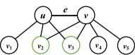
Local Counting (LC): For GPM problems that count matched embeddings instead of listing them, there may be no need to enumerate all matched embeddings since it may be possible to derive precise counts from counts of other patterns. Formally, the count of embeddings that match a pattern $\mathcal{P}$ may be calculated using the count of embeddings that match another pattern $\mathcal{P^{\prime}}$. This is useful when both patterns are being searched for or when one pattern is more efficient to search for than the other. This typically requires a local count (Pivoting, ) (or micro-level count (PGD, )) of embeddings associated with a single vertex or edge instead of a global count (or macro-level count) of embeddings that match the pattern.

Given a pattern $\mathcal{P}$ and a vertex $v$ (or an edge $e$) $\in G$, let $S$ be the set of all the embeddings of $\mathcal{P}$ in $G$. The local count of $\mathcal{P}$ on $v$ (or $e$) is defined as the number of subgraphs in $S$ that contains $v$ (or $e$). Fig. 6 shows an example of local counting on edge $e$. Given an edge $e:(u,v)$, the local count of $e$ for wedges $C_{wdg}(e)$ can be calculated from the local count of $e$ for triangles $C_{tri}(e)$ using this formula:

(1) $$C_{wdg}=(deg_{u}-C_{tri}-1)+(deg_{v}-C_{tri}-1)$$

$deg_{u}$ and $deg_{v}$ are the degrees of $u$ and $v$.

Since wedge counts can be computed from triangle counts, enumerating wedges is avoided when using local counting for 3-MC. Similar formulas can be applied for $k$-MC. Besides, local counting can also be used to prune the search space for many subgraph counting problems. For example, to count edge-induced diamonds, we first compute the local triangle count $n_{t}$ for each edge $e$, and use the formula $n_{t}\choose 2$ $=n_{t}\times(n_{t}-1)/2$ to get the local diamond count. The global diamond count is obtained by simply accumulating local counts.

Sandslash exposes localReduce (LABEL:lst:lo-api) to let the user specify how local counts are accumulated. Sandslash also exposes toExtend and toAdd to permit the user to customize the subgraph tree exploration so that the user can determine which patterns need to be enumerated. LABEL:lst:motif-opt in Appendix shows the user code for 3-MC using local counting. Sandslash activates local counting when the user implements localReduce.

Figure 7. Local graph induced by edge $(v_{5},v_{6})$ and common neighbors of $v_{5}$ and $v_{6}$ from the global graph.

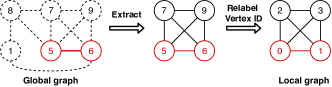
Search on Local Graph (LG) In some problems like $k$-CL, pattern invariants can be exploited to prune the search space (KClique, ). To extend an embedding {$v_{1}...v_{i}$} at level $i-1$ for $k$-CL, the baseline search strategy considers all the neighbors of these vertices in the input graph that are not already in the embedding. For $k$-CL, any successful candidate vertex for extension must be a neighbor of all $v_{i}$ (otherwise the extension will not result in a clique), so it is more efficient to intersect the neighbor lists of the $v_{i}$ and consider only the vertices in this intersection as candidates for vertex extension. Abstractly, this can be viewed as constructing a local graph that is the vertex-induced subgraph $G_{i}$ consisting of the vertices $v_{i}$ and the vertices in the intersection of their neighbor lists, and selecting candidate vertices only from $G_{i}$. Furthermore, if $v_{i+1}$ is the vertex selected at this stage, subgraph $G_{i+1}$ is obtained from $G_{i}$ by removing all vertices in $G_{i}$ that are not neighbors of $v_{i+1}$. In this way, the local graph keeps shrinking as the level increases, further reducing the search space. Fig. 7 illustrates an example of induced local graphs.

Sandslash allows the user specify how to initialize the local graph using initLG() and update it at the end of each DFS level using updateLG() (optional). When initLG() is defined, Sandslash enables LG to get the neighborhood information during extension using the local graph.

Graph	Source	# V	# E	$\overline{d}$	# Labels
Pa	Patents (Patent, )	3M	28M	10	37
Yo	Youtube (Youtube, )	7M	114M	16	29
Pdb	ProteinDB (DistGraph, )	49M	388M	8	25
Lj	LiveJournal (SNAP, )	5M	86M	18	0
Or	Orkut (SNAP, )	3M	234M	76	0
Tw4	Twitter40 (twitter40, )	42M	2,405M	29	0
Fr	Friendster (friendster, )	66M	3,612M	28	0
Uk	UK2007 (uk2007, )	106M	6,604M	31	0
Gsh	Gsh-2015 (gsh2015, )	988M	51,381M	52	0

Table 4. Input graphs (symmetric, no loops, no duplicate edges, neighbor list sorted) and their properties ($\overline{d}$ is the average degree).

6. Evaluation

We present experimental setup in Section 6.1 and then compare Sandslash with state-of-the-art GPM systems and expert-optimized implementations in Section 6.2. Finally, Sandslash is analyzed in more detail in Sections 6.3.

6.1. Experimental Setup

We evaluate two variants of Sandslash: Sandslash-Hi, which only enables high-level optimizations, and Sandslash-Lo, which enables both high-level and low-level optimizations. We compare Sandslash with the state-of-the-art GPM systems: AutoMine (AutoMine, ), Pangolin (Pangolin, ), and Peregrine (Peregrine, ). We use the five applications (also used in previous systems) listed in Table 2. We also evaluate the state-of-the-art expert-optimized GPM applications (GAPBS, ; KClique, ; PGD, ; DistGraph, ) listed in Table 2 except for CECI (CECI, ) (not publicly available). For fair comparison, we modified DistGraph (DistGraph, ) and PGD (PGD, ) so that they produce the same output as Sandslash. We added a parameter $k$ in DistGraph: exploration stops when the pattern size becomes $k$. For PGD, we disabled counting disconnected patterns.

Table 4 lists the input graphs. The first 3 graphs (Pa, Yo, pdb) are vertex-labeled graphs which can be used for FSM. We also include widely used large graphs (Lj, Or, Tw4, Fr, Uk), and a very large web-crawl (gsh2015, ) (Gsh). These graphs do not have labels and are only used for TC, $k$-CL, SL, $k$-MC.

Our experiments were conducted on a 4 socket machine with Intel Xeon Gold 5120 2.2GHz CPUs (56 cores in total) and 190GB RAM. All runs use 56 threads. For the largest graph, Gsh, we used a 2 socket machine with Intel Xeon Cascade Lake 2.2 Ghz CPUs (48 cores in total) and 6TB of Intel Optane PMM (byte-addressable memory technology).

Peregrine preprocesses the input graph to reorder vertices based on their degrees, which can improve the performance of GPM applications. In our evaluation, Sandslash does not reorder vertices to be fair to other systems and hand-optimized applications which do not perform such preprocessing. We use a time-out of 30 hours, exclude graph loading and preprocessing time, and report results as an average of three runs.

6.2. Comparisons with Existing Systems

Recall that Tables 3(a) and 3(b) list the optimizations applicable for each GPM application and enabled by each GPM system.

Triangle Counting (TC): Note that BFS and DFS are similar for enumerating triangles. As shown in Table 5, Sandslash achieves competitive performance with Pangolin and expert-implemented GAP (GAPBS, ). Both Pangolin and Sandslash outperform Peregrine and AutoMine because they use DAG which is more efficient than on-the-fly symmetry breaking. On average, Sandslash outperforms AutoMine, Pangolin, Peregrine, and GAP by 10.1$\times$, 1.4$\times$, 13.8$\times$, and 1.4$\times$ respectively, for TC.

	Lj	Or	Tw4	Fr	Uk
Pangolin	0.4	2.3	75.5	55.1	45.8
AutoMine	1.1	6.4	9849.4	126.6	565.9
Peregrine	1.6	7.3	8492.4	100.3	3640.9
GAP	0.3	2.7	65.8	77.0	48.1
Sandslash-Hi	0.3	1.8	57.2	44.9	24.5

Table 5. Execution time (sec) of TC.

	4-CL					5-CL
	Lj	Or	Tw4	Fr	Uk	Lj	Or	Fr
Pangolin	19.5	56.6	TO	564.1	TO	970.4	223.4	1704.4
AutoMine	11.0	32.9	67168.4	209.6	44666.6	575.6	170.1	389.0
Peregrine	15.9	73.7	TO	397.3	55808.4	520.8	782.1	957.6
kClist	1.2	2.5	1174.0	84.0	OOM	22.3	5.8	87.5
Sandslash-Hi	0.6	2.4	1676.8	166.2	2481.2	13.9	7.4	194.9
Sandslash-Lo	0.7	1.9	681.8	60.4	2451.7	14.2	4.8	64.3

Table 6. $k$-CL execution time (sec) (OOM: out of memory; TO: timed out).

$k$-Clique Listing ($k$-CL): Table 6 presents $k$-CL results. Pangolin (BFS-only) performs poorly as memoizing of neighborhood connectivity (MNC) can only be enabled in DFS. Peregrine does on-the-fly symmetry breaking (SB), but it does not construct and use DAG as in Pangolin and Sandslash. Therefore, Peregrine performs similarly to Pangolin although it is a DFS based system. AutoMine is slower than Sandslash because it does not do symmetry breaking. We observe that Sandslash-Hi is already significantly faster than all the previous GPM systems. Moreover, Sandslash-Lo achieves better performance than even expert-implemented kClist (KClique, ) by enabling search on a local graph (LG). There are some cases where Sandslash-Lo underperforms Sandslash-Hi. This is because searching on local graph requires computing/maintaining local graphs. When the search space is not reduced significantly, the overhead might outweigh the benefits. We explain this in detail in Section 6.3. On average, Sandslash-Lo outperforms AutoMine, Pangolin, Peregrine, and kClist by 21.0$\times$, 35.1$\times$, 31.1$\times$, and 1.4$\times$ respectively, for $k$-CL.

	3-MC					4-MC
	Lj	Or	Tw4	Fr	Uk	Lj	Or
Pangolin	10.8	96.5	TO	2460.1	23676.6	TO	TO
AutoMine	3.1	18.2	48901.7	352.8	4051.0	15529.7	90914.5
Peregrine	2.5	4.9	8447.4	165.3	3571.5	163.6	1701.4
PGD	11.2	42.5	OOM	OOM	OOM	192.8	4069.6
Sandslash-Hi	2.1	12.1	TO	723.7	4979.1	2366.2	30394.7
Sandslash-Lo	0.3	1.6	304.6	43.8	386.8	16.7	232.4

Table 7. $k$-MC execution time (sec) (OOM: out of memory; TO: timed out).

	diamond				4-cycle
	Lj	Or	Tw4	Fr	Lj	Or	Fr
Pangolin	92.3	884.5	TO	9301.6	553.5	13208.2	TO
Peregrine	5.4	10.2	20898.4	178.1	144.4	1867.2	32276.8
Sandslash-Hi	1.5	4.2	44659.5	284.2	6.3	79.0	20490.9

Table 8. Execution time (sec) of SL.

	3-FSM									4-FSM
	Pa			Yo			Pdb			Pa			Pdb
$\sigma_{min}$	500	1K	5K	500	1K	5K	500	1K	5K	10K	20K	30K	500	1K	5K
Pangolin	17.0	19.1	27.4	86.8	88.3	91.5	57.6	66.1	117.3	OOM	146.2	29.4	OOM	OOM	OOM
Peregrine	103.8	118.4	94.3	52.8	69.9	60.8	928.7	837.1	943.7	28301.0	4240.6	397.3	TO	TO	TO
DistGraph	13.1	13.0	14.1	OOM	OOM	OOM	253.9	278.8	239.8	120.7	58.01	25.1	OOM	OOM	OOM
Sandslash	3.5	3.8	6.1	81.0	80.8	82.8	46.5	40.0	44.5	102.3	108.4	43.7	200.2	198.0	195.1

Table 9. Execution time (sec) of $k$-FSM:- $\sigma_{min}$: minimum support (OOM: out of memory; TO: timed out).

Figure 8. $k$-MC speedup with memoization of embedding/neighborhood connectivity.

Figure 9. $k$-CL speedup by applying search on local graph.

Figure 10. Comparing search space (# of enumerated embeddings) of high- and low-level Sandslash.

$k$-Motif Counting ($k$-MC): Table 7 compares $k$-MC performance. Sandslash-Hi outperforms AutoMine due to symmetry breaking, and Sandslash-Lo is orders of magnitude faster than Sandslash-Hi due to the local counting optimization. Pangolin is particularly inefficient for 4-MC as it cannot memoize neighborhood connectivity (MNC). Sandslash-Hi and Sandslash-Lo count all patterns simultaneously, whereas Peregrine does counting for each pattern/motif one by one, which allows it apply optimizations for each pattern. Unlike Sandslash, Peregrine reorders vertices during preprocessing. Peregrine is faster than Sandslash-Hi likely due to these reasons. Sandslash-Lo is faster than Peregrine due to the formula-based local counting optimization, which cannot be supported in the Peregrine API. All optimizations in expert-implemented PGD (PGD, ) are enabled in Sandslash-Lo. Sandslash-Lo outperforms PGD because PGD does not apply symmetry breaking and has much larger enumeration space. On average, Sandslash-Lo outperforms AutoMine, Pangolin, Peregrine, and PGD by 27.2$\times$, 53.6$\times$, 8.6$\times$ and 17.9$\times$, respectively.

Subgraph Listing (SL): Table 8 presents SL results (AutoMine is omitted since it has vertex-induced subgraph counting, not SL). Sandslash outperforms all other systems, except Peregrine for the diamond pattern on Lj and Fr, which is probably because it reorders vertices during preprocessing. Pangolin on the other hand is much slower than the other systems as it does not support memoization of neighborhood connectivity (MNC) optimization. The MNC approach in Sandslash is more efficient than the vertex set buffering (VSB) in Peregrine as explained in Section 4.3: Peregrine must do neighborhood intersections to determine connectivity while Sandslash does not. On average, Sandslash outperforms Pangolin and Peregrine by 29.5$\times$ and 5.6$\times$ respectively.

$k$-Frequent Subgraph Mining ($k$-FSM): Table 9 presents $k$-FSM results (AutoMine is omitted because it does not use domain support for FSM). Although Peregrine uses DFS exploration, it does global synchronization among threads for each DFS iteration in FSM, which essentially results in BFS-like exploration. In contrast, Sandslash uses DFS exploration on the sub-pattern tree and filters patterns without synchronization. Peregrine is the fastest for Yo due to better load balance and relatively small number of frequent patterns. We observe that for graphs with a large number of frequent patterns (Pa), Peregrine becomes very inefficient as its pattern-centric approach enumerates all the possible patterns first and then enumerates embeddings for each pattern one by one; this is detrimental to performance for larger graphs and patterns (e.g., it times out for Pdb). Sandslash is similar or faster than Pangolin in most cases but is slower for Pa at $\sigma$=30K mainly because the BFS based approach has high parallelism for that case. For 4-FSM, Sandslash outperforms both Pangolin and Peregrine. Sandslash performs better than expert-implemented DistGraph (DistGraph, ) too as it automatically enables all optimizations that are in DistGraph. Sandslash is the only system that can run 4-FSM on Pdb. On average, Sandslash outperforms Pangolin, Peregrine, and DistGraph by 1.2$\times$, 4.6$\times$ and 2.4$\times$, respectively, for FSM.

6.3. Analysis of Sandslash

Due to lack of space, we present only the impact of optimizations in Sandslash that are missing in other systems (Table 3(b)).

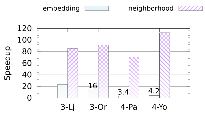
High-Level Optimizations: We observe 2% to 16% improvement for $k$-CL due to the degree filtering (DF) optimization. Fig. 10 shows speedup due to memoization of embedding connectivity (MEC) and memoization of neighborhood connectivity (MNC) optimizations for $k$-MC. For $k$-MC, the connectivity information in both the neighborhood and the embedding is memoized. MEC and MNC improve performance by 7.4$\times$ and 87$\times$ on average.

Low-Level Optimizations: Formula-based local counting (LC) reduces compute time by avoiding unnecessary enumeration of patterns. Table 7 shows Sandslash-Lo is 38$\times$ faster than Sandslash-Hi due to LC. As the pattern gets larger, pruning becomes more important. LC improves performance of 3-MC and 4-MC by 25$\times$ and 136$\times$ on average, respectively. This highlights the need to expose a low-level interface to express customized pruning strategies.

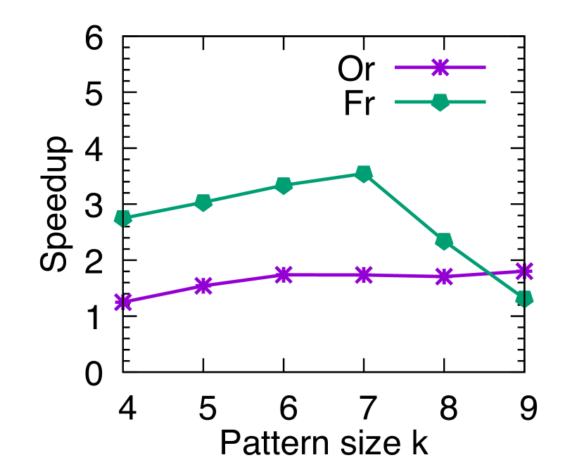
Fig. 10 illustrates the performance improvement on $k$-CL using the local graphs (LG) optimization on large patterns. Shrinking the local graph can reduce the search space compared to using the original graph. This improves performance by 1.2$\times$ to 3.5$\times$ for Or and Fr. The speedup for Or increases as the pattern size $k$ increases. However, for Fr, the speedup peaks at $k=7$, indicating that further shrinking becomes less effective as $k$ grows. This trend depends on the input graph topology, but in general, this optimization is effective for supporting large patterns.

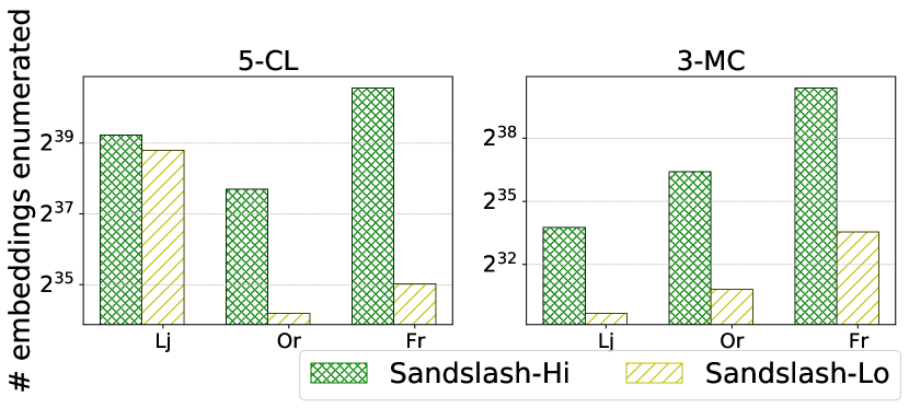
Both LC and LG optimizations prune the enumeration search space. We compare the search spaces of Sandslash-Hi and Sandslash-Lo to explain how they improve performance. Fig. 10 shows the number of enumerated embeddings for $k$-CL and $k$-MC. We observe a significant reduction for Or and Fr in Sandslash-Lo, explaining the performance differences between Sandslash-Hi and Sandslash-Lo in Tables 6 and 7. However, the pruning is less effective for Lj in $k$-CL, and given the overhead of local graph construction, Sandslash-Lo performs similar to Sandslash-Hi for Lj as shown in Table 6.

Figure 11. Execution time (sec in log scale) of $k$-CL on Fr graph.

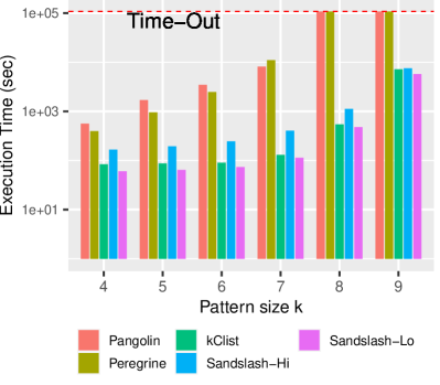
Large Patterns: Fig. 11 shows $k$-CL on Fr graph with $k$ from 4 to 9. Pangolin and Peregrine timed out for $k=8$ and $k=9$. Existing systems cannot efficiently mine large patterns due to a much larger enumeration search space or significant amount of redundant computation. In contrast, Sandslash can effectively handle these large patterns, and in all cases Sandslash-Lo is faster than expert-implemented kClist.

Large Inputs: The large input graph, Gsh, requires 199GB in Compressed Sparse Row (CSR) format on disk, so we evaluate it using 96 threads on the Optane machine. We were not able to run AutoMine and Peregrine on this large input. For 4-CL, Pangolin takes 6.5 hours, whereas Sandslash-Hi takes only 0.9 hours. Sandslash-Hi’s memory usage is low as well: peak memory usage for Sandslash-Hi is 436 GB, while Pangolin, a BFS-based system, uses 3.5 TB memory. kClist and Sandslash-Lo run out of memory because maintaining the local graphs consumes more than 6 TB memory.

Strong Scaling: The speedup of Sandslash on 56 threads over Sandslash on 1 thread is, on average, 43$\times$, 28$\times$, 39$\times$, 35$\times$, and 8$\times$ for TC, $k$-CL, SL, $k$-MC, and $k$-FSM, respectively. The speedup for $k$-FSM is lower due to constrained parallelism in traversing the sub-pattern tree. Sandslash balances work well because the number of grains/vertices is large enough. Orthogonal techniques like fine-grained work-stealing in Fractal and vertex reordering (preprocessing) in Peregrine can be added to Sandslash to further improve load balance.

7. Related Work

Low-level GPM Systems: Arabesque (Arabesque, ) is a distributed GPM system that proposed the embedding-centric programming paradigm. RStream (RStream, ) is an out-of-core GPM system on a single machine. Its programming model is based on relational algebra. Kaleido (Kaleido, ) is a single-machine system that uses a compressed sparse embedding (CSE) data structure to reduce memory consumption. G-Miner (G-Miner, ) is a distributed GPM system which incorporates task-parallel processing. Pangolin (Pangolin, ) is a shared-memory GPM system targeting both CPU and GPU. Instead of the BFS exploration used in the above systems, Fractal (Fractal, ) uses DFS to enumerate subgraphs on distributed platforms. Compared to these systems, Sandslash improves productivity and performance since many optimizations are automated in Sandslash. Some of these GPM systems use distributed, out-of-core, or GPU platforms, which is orthogonal to our work. The focus of our work is utilizing in-memory CPU platforms to get the best performance.

High-level GPM Systems: AutoMine (AutoMine, ) is a DFS based system targeting a single-machine. It provides a high-level programming interface and employs a compiler to generate high performance GPM programs. Sandslash supports a wider range of GPM problems and also enhances performance without compromising productivity. Peregrine is the state-of-the-art high-level GPM system. It includes efficient matching strategies from well-established techniques (Cartesian, ; DUALSIM, ; Breaking, ) and improves performance compared to previous systems. Nevertheless, Sandslash outperforms Peregrine using only its high-level API. Furthermore, Sandslash provides a low-level API to trade-off programming effort for much better performance.

GPM Algorithms: There are numerous hand-optimized GPM applications targeting various platforms. For TC, there are parallel solvers on multicore CPUs (Shun, ; GBBS, ; TC2017, ; TC2018, ), distributed CPUs (Suri, ; PDTL, ; TC2019, ), and GPUs (TriCore, ; DistTC, ; H-INDEX, ). kClist (KClique, ) is a parallel $k$-CL algorithm derived from (Arboricity, ). It constructs DAG using a core value based ordering to reduce search space. PGD (PGD, ) counts 3 and 4-motifs by leveraging proven formulas to reduce enumeration space. Escape (ESCAPE, ) extends this approach to 5-motifs. Subgraph listing (Ullmann, ; PSgL, ; CECI, ; DUALSIM, ; Cartesian, ; PathSampling, ; TurboFlux, ; Ma, ; Lai, ; Scaling, ; FRDSE, ; EPSE, ; Graphflow, ; WCOJ, ; EmptyHeaded, ) is another important application in which a matching order is applied to reduce search space and avoid graph isomorphism tests. gSpan (gSpan, ) is a sequential FSM algorithm using a lexicographic order for symmetry breaking. DistGraph (DistGraph, ; ParFSM, ) parallelizes gSpan with a customized dynamic load balancer that splits tasks on the fly. We did holistic analysis on the optimizations introduced in these expert-written solvers and implemented them in Sandslash for better productivity.

8. Conclusion

In this work, We present Sandslash, a two-level shared-memory GPM system that provides high productivity and high performance without compromising expressiveness. The user can easily compose GPM applications with the support of automated optimizations and transparent parallelism. The system also gives the user flexibility to express advanced optimizations to boost performance further. Sandslash significantly outperforms existing systems and even hand-optimized implementations.

Appendix A Pseudo Code in Low-level Sandslash

⬇

1void localReduce(int depth, vector<Support> &supports) {

2 // accumulate local wedge count for each vertex

3 if (depth == 0) {

4 Vertex v = getHistory(depth);

5 int n = getDegree(v);

6 int pid = getWedgePid();

7 supports[pid] += n * (n-1) / 2;

8 }

9}

10Pattern p = generateTriangle();

11Support tri_count = enumerate(p);

12int pid = getTrianglePid();

13supports[pid] = tri_count; // global triangle count

14pid = getWedgePid();

15supports[pid] -= 3 * tri_count; // global wedge count

Listing 2: Sandslash-Lo user code for 3-MC using local counting.

⬇

1void localReduce(int depth, vector<Support> &supports) {

2 // accumulate local counts for each edge

3 if (depth == 1) {

4 Vertex u = getHistory(0);

5 Vertex v = getHistory(1);

6 int deg_u = getDegree(u);

7 int deg_v = getDegree(v);

8 int tri = intersection_num(u, v);

9 int staru = deg_u - tri - 1;

10 int starv = deg_v - tri - 1;

11 int pid = getDiamondPid();

12 supports[pid] += tri * (tri - 1);

13 pid = getTailedTrianglePid();

14 supports[pid] += tri * (staru + starv);

15 pid = get4PathPid();

16 supports[pid] += staru * starv;

17 pid = get3StarPid();

18 supports[pid] += staru * (staru - 1) + starv * (starv - 1);

19 }

20}

21Pattern p0 = generateClique(4);

22Pattern p1 = generateCycle(4);

23Set<Pattern> patterns({p0, p1});

24Map<Pattern, Support> support_map = enumerate(patterns);

25...

Listing 3: Sandslash-Lo user code for 4-MC using local counting.

⬇

1// initialize the local graph by computing the

2// intersection of v’s neighbors and u’s neighbors,

3// where v is the start vertex, u is a neighbor of v’s.

4void initLG(Graph gg, Vertex v, Graph lg) {

5 for (u : gg.adjList(v))

6 lg.insertVertex(u); // insert vertex u to the local graph

7 // the system maintains the global to local ID mapping

8 for (u : gg.adjList(v))

9 for (w : (gg.adjList(u) & gg.adjList(v)))

10 lg.insertEdge(u, w); // insert edge (u, w) to local graph

11}

12// update the local graph by removing vertices not in

13// the newly generated embedding list

14void updateLG(int depth, Graph lg) {

15 // for each vertex in the new embedding list

16 for (u : this->emb_list[depth+1]) {

17 // get the size of the old adjList

18 int degree = lg.getDegree(depth, u);

19 int idx = lg.edgeStart(u);

20 int tail = eid + degree;

21 // set the size of the new adjList to 0

22 lg.setDegree(depth+1, u, 0);

23 // traverse the neighbors of u

24 for (w : lg.adjList(u)) {

25 // if w is in the new embedding list

26 if (this->emb_list[depth+1].contains(w)) {

27 // w remains in the new adjList of u

28 // size of u’s new adjList increases by 1

29 lg.incDegree(depth+1, u);

30 } else {

31 // remove w by swap it with

32 // the vertex at the tail of the old adjList

33 lg.insertAdj(idx--, lg.getEdgeDst(tail--);

34 lg.insertAdj(tail, w);

35 }

36 idx ++;

37 }

38 }

39}

Listing 4: Sandslash-Lo user code for $k$-CL using the local graph.

Appendix B Details of Optimizations and Definitions

B.1. Symmetry Breaking (Partial Order)

The problem of overcounting is circumvented by an automorphism check which selects a canonical representation from identical subgraphs. This technique is also known as symmetry breaking. A widely used approach is to apply partial orders between vertices in the embedding [32, 29]. For special patterns, e.g., cliques, symmetry breaking can be done by constructing a DAG, which avoids runtime checks but requires preprocessing. Sandslash supports both techniques and adaptively applies them according to the detected pattern. In  Fig. 2, lightly colored subgraphs are removed by automorphism checks, leaving a unique canonical subgraph for each set of automorphisms. Automorphism checks are also useful for pruning the search tree, e.g., the subgraph (2,1) is not extended in Fig. 2 because it is automorphic to the subgraph (1,2). High-level Sandslash enumerates only canonical embeddings, while low-level Sandslash allows user-defined automorphism check.

B.2. Orientation (Total Order)

The technique establishes a total ordering among vertices, and converts the input graph into a Directed Acyclic Graph (DAG). The search is then done over this DAG instead of the original input graph, which substantially reduces the search space. In Sandslash, orientation is automatically enabled when Sandslash detects a clique as the input pattern, i.e., when $|E|=|V|\times(|V|-1)/2$ for a given pattern $P(V,E)$. Currently two types of orientation schemes are supported: (1) degree based and (2) core value based. For degree based orientation, the ordering among vertices is established based on their degrees: each edge points towards the vertex with higher degree. When there is a tie, the edge points to the vertex with larger vertex ID. For core value based orientation, ordering is established using the core value of vertices [16], instead of degrees. It saves memory for local graph search, but requires more pre-processing time than the degree based orientation.

Figure 12. Possible matching orders for pattern diamond. The number in each vertex is not a vertex ID but the order being matched. Colors show the symmetric positions. The matching process can start from blue vertices (a & b & c) or green vertices (d & e). Among them, (a) and (e) match a wedge first, and then form a diamond; (b) (c) and (d) discover a triangle first, and then form a diamond.

B.3. Pattern-Guided Search (Matching Order)

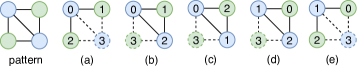
The pattern structure can be leveraged to prune the search space, which is known as matching-order. Fig. 12 shows the 5 possible matching orders for diamond. We can find the triangle first, and then add the fourth vertex connected to two of the endpoints of the triangle. Another possible matching order is to find a wedge first, and then find the fourth vertex that is connected to all three vertices of the wedge. Both orders find the diamond, but they explore different parts of the search space. In real-world sparse graphs, the number of wedges is usually orders-of-magnitude larger than the number of triangles, so it is more efficient to find the triangle first.

In general, using the right matching order reduces computation and memory consumption. Sandslash uses a greedy approach [32] to choose a good matching order: at each step, (1) we choose a sub-pattern which has more internal partial orders; (2) If there is a tie, we choose a denser sub-pattern, i.e., one with more edges. In Fig. 12, (c) is the matching order chosen by the system, since there is a partial order between vertex 0 and 1 for symmetry breaking (B.1). The intuition is that applying partial ordering as early as possible can better prune the search tree. Similarly, matching denser sub-pattern first can possibly prune more branches at early stage.

Note that using matching order avoids isomorphism test if the patterns are explicit. However, for implicit-pattern problems, this approach needs to enumerate all the possible patterns before search. For example, FSM in AutoMine generates a matching order for each unlabeled pattern and includes a lookup table to distinguish between labeled patterns. This table is massive when the graph has many distinct labels. Peregrine also suffers significant overhead for FSM since there are many patterns and it matches each of them one by one.

B.4. Fine-Grained Pruning

Many GPM algorithms use their own pruning strategy during the tree search, which significantly reduces the search space. Sandslash exposes toAdd and toExtend to allow fine-grained control on the pruning strategies. For example, in $k$-CL [16], since an $i$-clique can only be extended from an ($i$-1)-clique, toExtend and toAdd can be used to only extend the last vertex in the embedding and check if the newly added vertex is connected to all previous vertices in the embedding, respectively. In general, these two functions are used to specify the matching order and partial orders for explicit-pattern problems. The matching order is described by toExtend which specifies the next vertex to extend in each level. Connectivity and partial orders are checked in toAdd. Sandslash generates these functions automatically for explicit-pattern problems.

B.5. Customized Pattern Classification

To recognize the pattern of a given embedding, a straightforward approach is the graph isomorphism test, which is an expensive computation. To avoid the test, Sandslash uses matching order for explicit patterns. For multiple explicit pattern problems, the connectivity check can be used to identify different patterns. For small implicit patterns, Sandslash uses customized pattern classification (CP) [12]. For example, in FSM, the labeled wedge patterns can be differentiated by hashing the labels of the three vertices (the two endpoints of the wedge are symmetric). To enable CP, the user needs to use the getPattern API function to implement a customized method.

B.6. Example for Connectivity Code

As shown in Fig. 13, if the bit at position $i$ of connectivity code is set, there is an edge in $G$ between vertex $u$ and the vertex contained in the ancestor at level $i$ in the tree.

Figure 13. Example of the connectivity code. The code of $v_{2}$ is {1}, indicating $v_{2}$ is connected with $v_{1}$. $v_{4}$ has a code of {1,0,1}, meaning $v_{4}$ is connected to $v_{1}$ and $v_{3}$, but not $v_{2}$. Concatenating codes of all vertices, we get the code of this embedding {111101}. With this code we can rebuild the exact structure of the embedding on the left.

B.7. Subgraphs, Subgraph Trees and Patterns

The following definitions are standard [25]. Given a graph $G(V,E)$, a subgraph $G^{\prime}(V^{\prime},E^{\prime})$ of $G$ is a graph where $V^{\prime}\subseteq V$, $E^{\prime}\subseteq E$. If $G_{1}$ is a subgraph of $G_{2}$, we denote it as $G_{1}\subseteq G_{2}$.

Given a vertex set $W\subseteq V$, the vertex-induced subgraph is the graph $G^{\prime}$ whose (1) vertex set is $W$ and whose (2) edge set contains the edges in $E$ whose endpoints are in $W$. Given an edge set $F\subseteq E$, the edge-induced subgraph is the graph $G^{\prime}$ whose (1) edge set is $F$ and whose (2) vertex set contains the endpoints in $V$ of the edges in $F$. The difference between the two types of subgraphs can be understood as follows. Suppose vertices $v_{1}$ and $v_{2}$ are connected by an edge $e$ in $G$. If $v_{1}$ and $v_{2}$ occur in a vertex-induced subgraph, then $e$ occurs in the subgraph as well; in an edge-induced subgraph, edge $e$ will be present only if it is in the given edge set $F$. Any vertex-induced subgraph can be formulated as an edge-induced subgraph.

Two graphs $G_{1}(V_{1},E_{1})$ and $G_{2}(V_{2},E_{2})$ are isomorphic, denoted $G_{1}\simeq G_{2}$, if there exists a bijection $\mathbf{f}$: $V_{1}\rightarrow V_{2}$, such that any two vertices $u$ and $v$ of $G_{1}$ are adjacent in $G_{1}$ if and only if $\mathbf{f}(u)$ and $\mathbf{f}(v)$ are adjacent in $G_{2}$. In other words, $G_{1}$ and $G_{2}$ are structurally identical. In the case when $\mathbf{f}$ is a mapping of a graph onto itself, i.e., when $G_{1}$ and $G_{2}$ are the same graph, $G_{1}$ and $G_{2}$ are automorphic, i.e. $G_{1}\cong G_{2}$.

References

- [1] Christopher R. Aberger, Andrew Lamb, Susan Tu, Andres Nötzli, Kunle Olukotun, and Christopher Ré. Emptyheaded: A relational engine for graph processing. ACM Trans. Database Syst., 42(4), October 2017.
- [2] Charu C. Aggarwal and Haixun Wang. Managing and Mining Graph Data. Springer US, 2010.
- [3] Nesreen K. Ahmed, Jennifer Neville, Ryan A. Rossi, and Nick Duffield. Efficient graphlet counting for large networks. In ICDM, pages 1–10, 2015.
- [4] N. Alon, P. Dao, I. Hajirasouliha, F. Hormozdiari, and SC. Sahinalp. Biomolecular network motif counting and discovery by color coding. Bioinformatics, 24(13):241–249, 2008.
- [5] Scott Beamer, Krste Asanovic, and David A. Patterson. The GAP benchmark suite. CoRR, abs/1508.03619, 2015.
- [6] Austin R. Benson, David F. Gleich, and Jure Leskovec. Higher-order organization of complex networks. Science, 353(6295):163–166, 2016.
- [7] Bibek Bhattarai, Hang Liu, and H. Howie Huang. CECI: Compact Embedding Cluster Index for Scalable Subgraph Matching. In Proceedings of the 2019 International Conference on Management of Data, SIGMOD ’19, pages 1447–1462, New York, NY, USA, 2019. ACM.
- [8] Fei Bi, Lijun Chang, Xuemin Lin, Lu Qin, and Wenjie Zhang. Efficient subgraph matching by postponing cartesian products. In Proceedings of the 2016 International Conference on Management of Data, SIGMOD ’16, page 1199–1214, New York, NY, USA, 2016. Association for Computing Machinery.
- [9] Paolo Boldi, Massimo Santini, and Sebastiano Vigna. A large time-aware graph. SIGIR Forum, 42(2):33–38, 2008.
- [10] Paolo Boldi and Sebastiano Vigna. The WebGraph framework I: Compression techniques. In Proc. of the Thirteenth International World Wide Web Conference (WWW 2004), pages 595–601, Manhattan, USA, 2004. ACM Press.
- [11] Hongzhi Chen, Miao Liu, Yunjian Zhao, Xiao Yan, Da Yan, and James Cheng. G-miner: An efficient task-oriented graph mining system. In Proceedings of the Thirteenth EuroSys Conference, EuroSys ’18, New York, NY, USA, 2018. Association for Computing Machinery.
- [12] Xuhao Chen, Roshan Dathathri, Gurbinder Gill, and Keshav Pingali. Pangolin: An efficient and flexible graph mining system on cpu and gpu. Proc. VLDB Endow., 13(8), August 2020.
- [13] X. Cheng, C. Dale, and J. Liu. Dataset for statistics and social network of youtube videos. http://netsg.cs.sfu.ca/youtubedata/.
- [14] Norishige Chiba and Takao Nishizeki. Arboricity and subgraph listing algorithms. SIAM J. Comput., 14(1):210–223, February 1985.
- [15] Young-Rae Cho and Aidong Zhang. Predicting protein function by frequent functional association pattern mining in protein interaction networks. Trans. Info. Tech. Biomed., 14(1):30–36, January 2010.
- [16] Maximilien Danisch, Oana Balalau, and Mauro Sozio. Listing k-cliques in sparse real-world graphs*. In Proceedings of the 2018 World Wide Web Conference, WWW ’18, pages 589–598, Republic and Canton of Geneva, Switzerland, 2018. International World Wide Web Conferences Steering Committee.
- [17] M. Deshpande, M. Kuramochi, N. Wale, and G. Karypis. Frequent substructure-based approaches for classifying chemical compounds. IEEE Transactions on Knowledge and Data Engineering, 17(8):1036–1050, Aug 2005.
- [18] Laxman Dhulipala, Guy E. Blelloch, and Julian Shun. Theoretically efficient parallel graph algorithms can be fast and scalable. In Proceedings of the 30th on Symposium on Parallelism in Algorithms and Architectures, SPAA ’18, page 393–404, New York, NY, USA, 2018. Association for Computing Machinery.
- [19] Vinicius Dias, Carlos H. C. Teixeira, Dorgival Guedes, Wagner Meira, and Srinivasan Parthasarathy. Fractal: A general-purpose graph pattern mining system. In Proceedings of the 2019 International Conference on Management of Data, SIGMOD ’19, pages 1357–1374, New York, NY, USA, 2019. ACM.
- [20] Katherine Faust. A puzzle concerning triads in social networks: Graph constraints and the triad census. Social Networks, 32(3):221 – 233, 2010.
- [21] Brian Gallagher. Matching structure and semantics: A survey on graph-based pattern matching. In AAAI Fall Symposium: Capturing and Using Patterns for Evidence Detection, 2006.
- [22] I. Giechaskiel, G. Panagopoulos, and E. Yoneki. PDTL: Parallel and distributed triangle listing for massive graphs. In 2015 44th International Conference on Parallel Processing, pages 370–379, Sep. 2015.
- [23] Joshua A. Grochow and Manolis Kellis. Network motif discovery using subgraph enumeration and symmetry-breaking. In Proceedings of the 11th Annual International Conference on Research in Computational Molecular Biology, RECOMB’07, page 92–106, Berlin, Heidelberg, 2007. Springer-Verlag.
- [24] B. H. Hall, Jaffe A. B., and Trajtenberg M. The NBER patent citation data file: Lessons, insights and methodological tools. http://www.nber.org/patents/, 2001.
- [25] F. Harary. Graph theory. Addison-Wesley series in mathematics. Addison-Wesley Pub. Co., 1969.
- [26] Loc Hoang, Vishwesh Jatala, Xuhao Chen, Udit Agarwal, Roshan Dathathri, Gurbinder Gill, and Keshav Pingali. DistTC: High performance distributed triangle counting. In HPEC 2019 23rd IEEE High Performance Extreme Computing, Graph Challenge, September 2019.
- [27] Y. Hu, H. Liu, and H. H. Huang. Tricore: Parallel triangle counting on gpus. In SC18: International Conference for High Performance Computing, Networking, Storage and Analysis, pages 171–182, Nov 2018.
- [28] Shweta Jain and C. Seshadhri. The power of pivoting for exact clique counting. In Proceedings of the 13th International Conference on Web Search and Data Mining, WSDM ’20, page 268–276, New York, NY, USA, 2020. Association for Computing Machinery.
- [29] Kasra Jamshidi, Rakesh Mahadasa, and Keval Vora. Peregrine: A pattern-aware graph mining system. In Proceedings of the Fifteenth EuroSys Conference, EuroSys ’20, 2020.
- [30] Madhav Jha, C. Seshadhri, and Ali Pinar. Path sampling: A fast and provable method for estimating 4-vertex subgraph counts. In Proceedings of the 24th International Conference on World Wide Web, WWW ’15, pages 495–505, Republic and Canton of Geneva, Switzerland, 2015. International World Wide Web Conferences Steering Committee.
- [31] Chathura Kankanamge, Siddhartha Sahu, Amine Mhedbhi, Jeremy Chen, and Semih Salihoglu. Graphflow: An active graph database. In Proceedings of the 2017 ACM International Conference on Management of Data, SIGMOD ’17, page 1695–1698, New York, NY, USA, 2017. Association for Computing Machinery.
- [32] Hyeonji Kim, Juneyoung Lee, Sourav S. Bhowmick, Wook-Shin Han, JeongHoon Lee, Seongyun Ko, and Moath H.A. Jarrah. DUALSIM: Parallel subgraph enumeration in a massive graph on a single machine. In Proceedings of the 2016 International Conference on Management of Data, SIGMOD ’16, pages 1231–1245, New York, NY, USA, 2016. ACM.
- [33] Kyoungmin Kim, In Seo, Wook-Shin Han, Jeong-Hoon Lee, Sungpack Hong, Hassan Chafi, Hyungyu Shin, and Geonhwa Jeong. Turboflux: A fast continuous subgraph matching system for streaming graph data. In Proceedings of the 2018 International Conference on Management of Data, SIGMOD ’18, pages 411–426, New York, NY, USA, 2018. ACM.
- [34] Haewoon Kwak, Changhyun Lee, Hosung Park, and Sue Moon. What is twitter, a social network or a news media? In Proceedings of the 19th International Conference on World Wide Web, WWW ’10, pages 591–600, New York, NY, USA, 2010. ACM.
- [35] Longbin Lai, Lu Qin, Xuemin Lin, and Lijun Chang. Scalable subgraph enumeration in mapreduce. Proc. VLDB Endow., 8(10):974–985, June 2015.
- [36] J. Leskovec. Snap: Stanford network analysis platform, 2013.
- [37] Shuai Ma, Yang Cao, Jinpeng Huai, and Tianyu Wo. Distributed graph pattern matching. In Proceedings of the 21st International Conference on World Wide Web, WWW ’12, pages 949–958, New York, NY, USA, 2012. ACM.
- [38] Daniel Mawhirter, Sam Reinehr, Connor Holmes, Tongping Liu, and Bo Wu. Graphzero: Breaking symmetry for efficient graph mining, 2019.
- [39] Daniel Mawhirter and Bo Wu. Automine: Harmonizing high-level abstraction and high performance for graph mining. In Proceedings of the 27th ACM Symposium on Operating Systems Principles, SOSP ’19, pages 509–523, New York, NY, USA, 2019. ACM.
- [40] Amine Mhedhbi and Semih Salihoglu. Optimizing subgraph queries by combining binary and worst-case optimal joins. Proc. VLDB Endow., 12(11):1692–1704, July 2019.
- [41] R. Milo, S. Shen-Orr, S. Itzkovitz, N. Kashtan, D. Chklovskii, and U. Alon. Network motifs: Simple building blocks of complex networks. Science, 298(5594):824–827, 2002.
- [42] Donald Nguyen, Andrew Lenharth, and Keshav Pingali. A lightweight infrastructure for graph analytics. In Proceedings of the 24th ACM Symposium on Operating Systems Principles (SOSP), SOSP ’13, pages 456–471, New York, NY, USA, 2013. ACM.
- [43] Santosh Pandey, Xiaoye Sherry Li, Aydin Buluc, Jiejun Xu, and Hang Liu. H-index: Hash-indexing for parallel triangle counting on gpus. In 2019 IEEE High Performance Extreme Computing Conference (HPEC), pages 1–7. IEEE, Sep. 2019.
- [44] Roger Pearce, Trevor Steil, Benjamin W Priest, and Geoffrey Sanders. One quadrillion triangles queried on one million processors. In 2019 IEEE High Performance Extreme Computing Conference (HPEC), pages 1–5. IEEE, 2019.
- [45] Ali Pinar, C. Seshadhri, and Vaidyanathan Vishal. Escape: Efficiently counting all 5-vertex subgraphs. In Proceedings of the 26th International Conference on World Wide Web, WWW ’17, pages 1431–1440, Republic and Canton of Geneva, Switzerland, 2017. International World Wide Web Conferences Steering Committee.
- [46] Xuguang Ren, Junhu Wang, Wook-Shin Han, and Jeffrey Xu Yu. Fast and robust distributed subgraph enumeration. Proceedings of the VLDB Endowment, 12(11):1344–1356, 2019.
- [47] Yingxia Shao, Bin Cui, Lei Chen, Lin Ma, Junjie Yao, and Ning Xu. Parallel subgraph listing in a large-scale graph. In Proceedings of the 2014 ACM SIGMOD International Conference on Management of Data, SIGMOD ’14, pages 625–636, New York, NY, USA, 2014. ACM.
- [48] J. Shun and K. Tangwongsan. Multicore triangle computations without tuning. In 2015 IEEE 31st International Conference on Data Engineering, pages 149–160, April 2015.
- [49] Shixuan Sun, Yulin Che, Lipeng Wang, and Qiong Luo. Efficient parallel subgraph enumeration on a single machine. In 2019 IEEE 35th International Conference on Data Engineering (ICDE), pages 232–243. IEEE, 2019.
- [50] Shixuan Sun and Qiong Luo. Scaling up subgraph query processing with efficient subgraph matching. In 2019 IEEE 35th International Conference on Data Engineering (ICDE), pages 220–231. IEEE, 2019.
- [51] Siddharth Suri and Sergei Vassilvitskii. Counting triangles and the curse of the last reducer. In Proceedings of the 20th International Conference on World Wide Web, WWW ’11, pages 607–614, New York, NY, USA, 2011. ACM.
- [52] N. Talukder and M. J. Zaki. A distributed approach for graph mining in massive networks. Data Min. Knowl. Discov., 30(5):1024–1052, September 2016.
- [53] N. Talukder and M. J. Zaki. Parallel graph mining with dynamic load balancing. In 2016 IEEE International Conference on Big Data (Big Data), pages 3352–3359, Dec 2016.
- [54] Carlos H. C. Teixeira, Alexandre J. Fonseca, Marco Serafini, Georgos Siganos, Mohammed J. Zaki, and Ashraf Aboulnaga. Arabesque: A system for distributed graph mining. In Proceedings of the 25th Symposium on Operating Systems Principles, SOSP ’15, pages 425–440, New York, NY, USA, 2015. ACM.
- [55] J. R. Ullmann. An algorithm for subgraph isomorphism. J. ACM, 23(1):31–42, January 1976.
- [56] Kai Wang, Zhiqiang Zuo, John Thorpe, Tien Quang Nguyen, and Guoqing Harry Xu. Rstream: Marrying relational algebra with streaming for efficient graph mining on a single machine. In Proceedings of the 12th USENIX Conference on Operating Systems Design and Implementation, OSDI’18, pages 763–782, Berkeley, CA, USA, 2018. USENIX Association.
- [57] Michael M Wolf, Mehmet Deveci, Jonathan W Berry, Simon D Hammond, and Sivasankaran Rajamanickam. Fast linear algebra-based triangle counting with kokkoskernels. In 2017 IEEE High Performance Extreme Computing Conference (HPEC), pages 1–7. IEEE, 2017.
- [58] Xifeng Yan and Jiawei Han. gspan: graph-based substructure pattern mining. In Proceedings of the 2002 IEEE International Conference on Data Mining, pages 721–724, Dec 2002.
- [59] Jaewon Yang and Jure Leskovec. Defining and evaluating network communities based on ground-truth. CoRR, abs/1205.6233, 2012.
- [60] Abdurrahman Yaşar, Sivasankaran Rajamanickam, Michael Wolf, Jonathan Berry, and Ümit V Çatalyürek. Fast triangle counting using cilk. In 2018 IEEE High Performance extreme Computing Conference (HPEC), pages 1–7. IEEE, 2018.
- [61] Cheng Zhao, Zhibin Zhang, Peng Xu, Tianqi Zheng, and Jiafeng Guo. Kaleido: An Efficient Out-of-core Graph Mining System on A Single Machine. In Proceedings of the 2020 IEEE International Conference on Data Engineering (ICDE 2020), ICDE ’20, 2020.