Supporting Information

Deep generative selection models of T and B cell receptor repertoires with soNNia
Giulio Isacchini, Aleksandra M. Walczak, Thierry Mora, Armita Nourmohammad

Contents

1. 1 SoNNia
2. 2 Pre-processing steps
3. 3 Generation model
4. 4 Neural network architectures
5. 5 soNNia model inference
6. 6 Hierarchy of models in linear SONIA
7. 7 Transfer Learning
8. 8 Estimation of information theoretic quantities

1 SoNNia

SoNNia is a python software which extends the functionality of the SONIA package, using deep neural network architectures. It expands the choice of selection models to infer, by adding non-linear single-chain models and non-linear paired-chain models. Like other deep neural network algorithms, soNNia is powerful when trained on large datasets. While the use of appropriate regularization could reduce the risk of overfitting, it is recommended that the linear SONIA model is used for datasets with fewer than $10^{5}$ receptor sequences.

The pre-processing pipeline implemented in this paper is also included in the soNNia package as a separate class. The software is available on GitHub at https://github.com/statbiophys/soNNia.

2 Pre-processing steps

The standard pre-processing pipeline, which is implemented in the soNNia package and is applied to all datasets, consists of the following steps:

1. Select species and chain type

2. Verify sequences are written as V gene, CDR3 sequence, J gene and remove sequences with unknown genes and pseudogenes

3. Filter productive CDR3 sequences (lack of stop codons and nucleotide sequence length is a multiple of 3)

4. Filter sequences starting with a cysteine

5. Filter sequences with CDR3 amino acid length smaller than a maximum value (set to 30 in this paper)

6. Remove sequences with small read counts (optional).

For the analysis of Fig. 2 we analysed data from [1]. We first applied the standard pipeline. In addition we excluded TCRs with gene TRBJ2-5 which is badly annotated by the Adaptive pipeline [2] and removed a cluster of artefact sequences, which was previously identified in [3] and corresponds to the consensus sequence CFFKQKTAYEQYF.

For the analysis of Fig. 3 we analysed data from [4] and [5]. Dataset from  [4] was obtained already pre-processed directly from the authors, while pre-processed dataset from [5] is part of the supplementary material of the corresponding paper. The soNNia standard pipeline is then applied to both datasets, independently for each chain, and a pair is accepted only if it passes both filtering steps. For $\alpha$ TCR datasets, sequences carrying the following rare genes were removed due to their rarity in the out-of-frame dataset: TRAJ33, TRAJ38, TRAJ24, TRAV19.

For the analysis of Figs. 4 and 5 we analysed data from [6] and [7], to which we applied our standard pre-processing pipeline.

3 Generation model

The generation model relies on previously published models described in [8, 9, 10]. Briefly, the model is defined by the probability distributions of the various events involved in the VDJ recombination process: V, D, and J gene usage, and number of deletions and insertions at each junction. The model is learned from non-productive sequences using the IGoR software [9]. For BCR, only a few nonproductive sequences were available, and so we instead started from the default IGoR models learned elsewhere [9], and re-inferred only the V gene usage distribution for the heavy chain, and VJ joint gene distribution for light chains, keeping all other parameters fixed.

Amino-acid sequence probability computation and generation is done with the OLGA software, which relies on a dynamic programming approach. The process is applied to all $\alpha$, $\beta$, IgH and Ig$\kappa$/$\lambda$ chains. We focus on naive B cells and ignore somatic hypermutations. Since it was shown that individual variability in generation was only small [11], for each locus we used a single universal model.

4 Neural network architectures

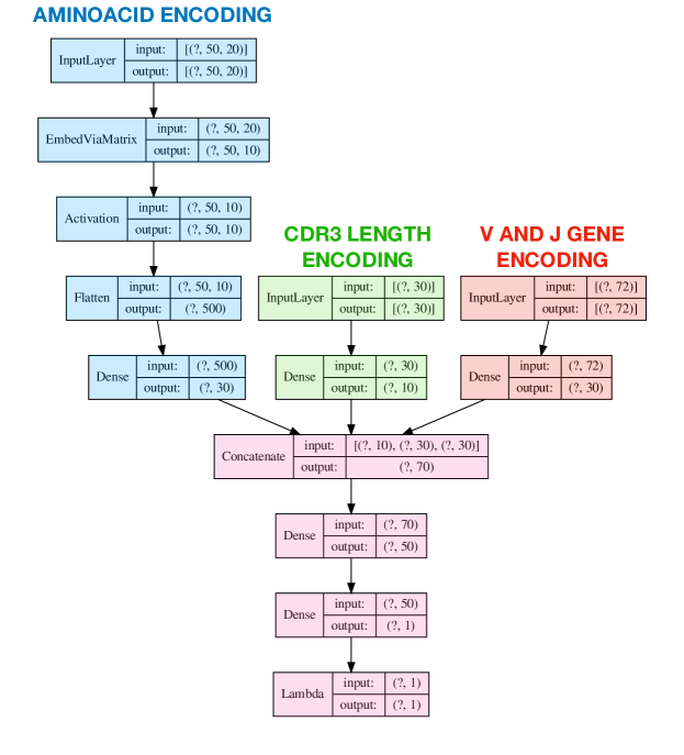
Figure S1: Neural network structure of the deep soNNia model for the single chain case. There are three inputs, from left to right: first the encoded aminoacid composition of the CDR3 using the left-right encoding scheme, then the length of the CDR3, finally the independent V and J gene usage information. The aminoacid input is encoded using an embedding layer, called EmbedViaMatrix and then processed by a tanh non-linearity, called Activation layer. The Flatten layer turns the encoded matrix in the corresponding flattened array where each row of the matrix is concatenated to the successive one. A dense layer is then applied to reduce its dimensionality. The other two inputs are also processed through a dense feed-forward layer to reduce their corresponding dimensionality. The three groups of encoded inputs are then concatenated and two dense feed forward layers are applied to output $\log Q$. Finally $\log Q$ is clipped to avoid diverging values using the Lambda layer.

We describe the architecture of the soNNia neural network. The input of our network is a vector $\mathbf{x}$ where $x_{f}=1$ (otherwise 0) if sequence $x$ has feature $f$. A dense layer is a map $\mathbf{L}(\mathbf{x})=\tanh(\mathbf{W}\mathbf{x}+\mathbf{b})$ with $\mathbf{x}$ the input vector, $\mathbf{W}$ the matrix of weights, $\mathbf{b}$ the vector bias, and where the $\tanh$ function is applied to each element of the input vector. The model architecture of the neural network is shown in Supplementary Fig. S1.The input is first subdivided into 3 sub-vectors: the $\mathbf{x}_{L}$ subset of features associated with CDR3 length, the $\mathbf{x}_{A}$ subset of features associated with the CDR3 amino acid composition and the $\mathbf{x}_{VJ}$ subset of features associated with V and J gene usage. We applied a dense layer individually to $\mathbf{x}_{L}$ and $\mathbf{x}_{VJ}$. In parallel, we performed an amino acid embedding of $\mathbf{x}_{A}$: we first reshape the vector to a $2K\times 20$ matrix $\mathbf{A}$ (the set of features associated with amino acid usage is $2\times K\times 20$ long, where $K=25$ the maximum distance from the left and right ends that we encode, and $20$ is the number of amino acids) and apply a linear embedding trough $\mathcal{M}(\mathbf{A})=\mathbf{A\mathbf{M}}$ with $\mathbf{M}$ a $20\times n$ matrix with $n$ the size of the amino acid encoding. We then flatten the matrix to an array and apply a dense layer. We merged the three transformed subsets into a vector and then applied a dense layer. We finally applied a last dense layer without non-linearity to produce the output value, $\log Q$(see Fig  S1).

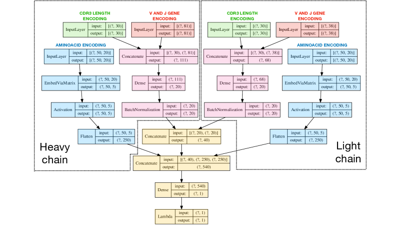
Figure S3: Neural Network structure of the deep-indep model for paired chains. See Fig. S1 for details on each layer.

The model for paired chains focuses on combining the $\mathbf{x}_{L}$ and $\mathbf{x}_{VJ}$ inputs of the two chains. First the $\mathbf{x}_{L}$ and $\mathbf{x}_{VJ}$ inputs within each chain are merged and processed with a dense layer. Subsequently a Batch Normalizing Transform is applied to each encoded vector to enforce a comparable contribution of each chain once the vectors are merged and processed through a dense layer (this last step is skipped in the deep-indep model). A Batch Normalizing Transform [12] is a differentiable operator which is normally used to improve performance, speed and stability of a Neural Network. Given a batch of data, it normalizes the input of a layer such that it will have mean output activation 0 and standard deviation of 1. In parallel, the amino acid inputs are embedded as described before. Finally all the vectors are merged together and a dense layer without activation outputs the $\log Q$ (see Fig  S3-4).

5 soNNia model inference

Given a sample of data sequences ${\mathcal{D}}=\{{\bf{x}}^{i}\}_{i=1}^{N_{D}}$ and a baseline ${\mathcal{G}}=\{{\bf{x}}^{\prime i}\}_{i=1}^{N_{G}}$ we want to maximize the average log-likelihood:

$$\begin{split}\mathcal{L}(\theta)&=\langle\log P_{\rm post}^{\theta}\rangle_{\mathcal{D}}=\frac{1}{N_{D}}\sum_{i=1}^{N_{D}}\log P_{\rm post}^{\theta}({\bf{x}}^{i})\\ &=\frac{1}{N_{D}}\sum_{i=1}^{N_{D}}[\log Q^{\theta}({\bf{x}}^{i})+\log P_{\rm gen}({\bf{x}}^{i})]-\log Z_{\theta}\\ &=\langle\log Q^{\theta}\rangle_{\mathcal{D}}+\langle\log P_{\rm gen}\rangle_{\mathcal{D}}-\log\langle Q^{\theta}\rangle_{{\mathcal{G}}},\end{split}$$ (S1)

where $Z_{\theta}=\langle Q^{\theta}\rangle_{\mathcal{G}}=N_{G}^{-1}\sum_{i=1}^{N_{G}}Q^{\theta}({\bf{x}}^{\prime i})$. The $P_{\rm gen}$ term in the last equation is parameter independent and can thus be discarded in the inference. When an empirical baseline is used, $P_{\rm gen}$ is replaced by $P_{\rm emp}({\bf{x}})=N_{G}^{-1}\sum_{i=1}^{N_{G}}\delta_{{\bf{x}},x^{\prime}_{i}}$. Otherwise, the baseline ${\mathcal{G}}$ is sampled from the $P_{\rm gen}$ model, which we learn from nonproductive sequences using the IGoR software [9].

The above likelihood is implemented in the soNNia inference procedure (linear and non-linear case) with the Keras [13] package. The model is invariant with respect to the transformation $Q({\bf{x}})\rightarrow cQ({\bf{x}})$ and $Z\rightarrow Z/c$, where c is an arbitrary constant, so we fix dynamically the gauge $Z=1$. We lift this degeneracy by adding the penalty $\Gamma(\theta)=(Z_{\theta}-1)^{2}$, and minimize $-\mathcal{L}_{sonia}(\theta)+\gamma\Gamma(\theta)$ with $\gamma=1$ as a loss function.

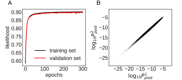
Figure S2: (A) Convergence of the training and validation likelihoods as a function of training epochs for the soNNia model shown in Fig. 2B. (B) Comparison between two soNNia models trained on independent datasets obtained by splitting the training set of $10^{7}$ TCR$\beta$ sequences pooled from repertoires of 743 individuals of ref. [1] (Fig. 2) in two equal parts.

In our implementation batch sizes between $10^{3}-10^{4}$ sequences produced a reliable inference. L2 and L1 regularization on kernel weights are also applied. Hyperparameters were chosen using a validation dataset of size 10 $\%$ of training data. The inference converges after around 100 epochs and the network does not overfit (Fig. S2A). To test the stability of our inference, we evaluated the $P_{\rm post}$ values of generated sequences, based on two models trained on subsets of the initial training data, and show that the $P_{\rm post}$ estimated are highly reproducible between these selection models (Fig S2B).

The left-right linear SONIA model contains an additional residual gauge, which makes the selection factor invariant with respect to the following transformation:

$$\begin{split}&q^{L}_{i}(a)\rightarrow\lambda_{i}q^{L}_{i}(a)\\ &q^{R}_{j}(a)\rightarrow\mu_{j}q^{R}_{j}(a)\\ &q_{\ell}\rightarrow q_{\ell}\prod_{i=\ell+1}^{\ell_{\text{max}}}\lambda_{i}\prod_{j=\ell+1}^{\ell_{\text{max}}}\mu_{j}\end{split}$$ (S2)

where $q^{L}_{i}(a)$ and $q^{R}_{j}(a)$ are respectively selection factors associated with the usage of amino acid $a$ at positions $i,j\in\{1,\dots,\ell_{\rm max}\}$ from the left and the right boundaries of CDR3 (Fig. 1D), and $q_{\ell}$ is the selection factor associated with CDR3 length $\ell$. The default value of $\ell_{\text{max}}$ is 25 aa in the left-right model for TCRs. We constrain the gauge by imposing $\sum_{a}P^{L}_{i,\mathcal{G}}(a)q^{L}_{i}(a)=1$ and $\sum_{a}P^{R}_{j,\mathcal{G}}(a)q^{R}_{j}(a)=1$ at all positions, similar to [14]. Here, $P^{L}_{i,\mathcal{G}}(a)$ and $P^{R}_{j,\mathcal{G}}(a)$ are the marginal probabilities for observing amino acid $a$ at respective positions $i$ (from the left) and $j$ (from the right) of CDR3 in the pre-selected ensemble $\mathcal{G}$ of sequences.

To learn the $Q_{\rm VJL}$ model of Fig. 4, we used a linear SONIA model where features $f$ where restricted to $V,J$ and CDR3 length features. One major difference with the approach of Ref. [15] is that, unlike the likelihood they use, we do not double-count the distribution of length (through $P(L|V)P(L|J)$). However, our results show that that error does not affect model performance substantially.

6 Hierarchy of models in linear SONIA

The linear SONIA model,

$$Q^{\theta}({\bf{x}})=e^{\sum_{f}\theta_{f}x_{f}},$$ (S3)

may be rationalized using the principle of minimum discriminatory information. In this scheme, we look for the distribution $P_{\rm post}$ that is most similar to our prior, described by the baseline set $P_{\rm gen}$ (or empirical set ${\mathcal{G}}$, replacing $P_{\rm gen}$ by $P_{\rm emp}({\bf{x}})=N_{G}^{-1}\sum_{i=1}^{N_{G}}\delta_{{\bf{x}},{\bf{x}}^{i}}$), but that still reproduces the marginal probabilities in the data. This translates to the minimization of the functional:

$$\begin{split}\mathcal{F}(P_{\rm post})&={D}_{\rm KL}(P_{\rm\rm post}\|P_{\rm gen})-\eta_{0}\Big{(}\sum_{{\bf{x}}}P_{\rm post}({\bf{x}})-1\Big{)}\\ &-\sum_{f}\theta_{f}\Big{(}P_{\rm post}(f)-P_{\rm data}(f)\Big{)},\end{split}$$ (S4)

where

$$D_{\rm KL}(P_{\rm\rm post}\|P_{\rm gen})\doteq\sum_{\bf{x}}P_{\rm\rm post}({\bf{x}})\log\frac{P_{\rm\rm post}({\bf{x}})}{P_{\rm gen}({\bf{x}})}.$$ (S5)

The second term on the right-hand side imposes the normalization of $P_{\rm post}$ and the last term imposes the constraint that the marginal probabilities of the selected set of features $f$ should match those in the data through the set of Lagrange multipliers $\theta_{f}$. This scheme reduces to the maximum entropy principle when ${\mathcal{G}}$ is uniformly distributed. Minimization of eq. S4 results in:

$$P_{\rm post}({\bf{x}})=\frac{e^{\sum_{f}\theta_{f}x_{f}}}{Z_{\theta}}P_{\rm gen}({\bf{x}}),$$ (S6)

where $Z_{\theta}=e^{1-\eta_{0}}$, which is equivalent to eq. S3. Because of the principle of Kullback-Leibler divergence minimization, adding new constraints on the features to the optimization necessary increases $D_{\rm KL}$. This allows us to define a hierarchy of models as we add new constraints.

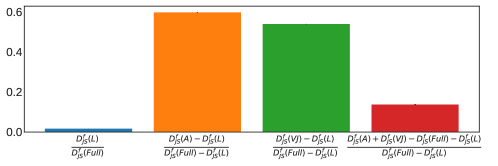
Figure S9: Decomposition of contribution from different features to the fractional Jensen Shannon divergence between the CD4 and CD8 subpertoire statistics, $D^{f}_{\rm JS}(L)\leq D_{\rm JS}^{f}(A),D_{\rm JS}^{f}(VJ)\leq D_{\rm JS}^{f}({\rm full})$. The blue bar is the contribution of CDR3 length; orange and green bars are the relative contributions from the amino-acid composition and VJ usage, respectively. Red bar is the fraction that’s redundant between VJ and amino acid usage. Contributions are balanced between amino acid and VJ usage, with moderate redundancy between the two.

To evaluate the relative contributions of each feature to the difference between CD4 and CD8 TCR, we define different models based on a baseline set ${\mathcal{G}}$ defined as empirical sequences, with (1) only CDR3 length features; (2) CDR3 length and amino acid features; (3) CDR3 length and VJ features; and (4) all features. We denote the corresponding KL divergences (eq. S5) $D_{\rm KL}^{r}(L)$, $D^{r}_{\rm KL}(A)$, $D^{r}_{\rm KL}(VJ)$, and $D^{r}_{\rm KL}({\rm full})$ for each subrepertoire $r=$CD4 or CD8, with $D^{r}_{\rm KL}({\rm full})\geq D^{r}_{\rm KL}(A),D^{r}_{\rm KL}(VJ)\geq D_{\rm KL}^{r}(L)$. In Fig. S9 each of these divergences are then combined to get a “fractional Jensen-Shannon” divergence $D^{f}_{\rm JS}=fD_{\rm KL}^{\rm CD4}+(1-f)D_{\rm KL}^{{\rm CD8}}$, where $f$ is the fraction of CD4 cells.

7 Transfer Learning

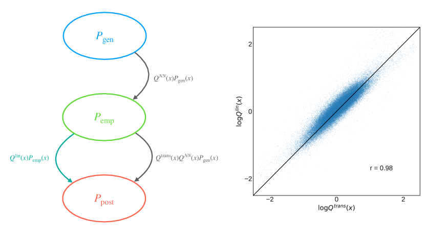
Figure S5: Transfer learning consists of a 2-step inference (left): in the first step we infer a deep neural network on a bigger data set ${\mathcal{G}}$, and in the second second step we re-infer a subsection of the network, or an additional layer on a smaller dataset, which is the real target. In our specific application, the big data ${\mathcal{G}}$ is the unfractioned repertoire from ref. [7] ($P_{\rm emp}({\bf{x}})=N_{G}^{-1}\sum_{i=1}^{N_{G}}\delta_{{\bf{x}},x^{\prime}_{i}}$), and the final targets are the sub-repertoires harvested from different tissues [6]. We can infer a deep selection model soNNia to characterize well the unfractioned repertoire $P_{\rm emp}$, and then learn a functional selection model for each sub-repertoire with an additional linear layer in the neural network. This procedure is equivalent to using $P_{\rm emp}$ as the baseline distribution in the inference of a linear selection model, as it can be seen by the high correlation between selection factors inferred with the two different methodologies (right).

Training a deep soNNia model (Fig. 1C) for each subset in the analysis of Fig. 4 leads to overfitting issues due to limited data. To solve this problem, we can use a mixture technique known as transfer learning (Fig. S5). Specifically, we first infer a deep soNNia model to characterize selection factors ($\mathcal{Q}^{\text{DNN}}(x)$) on unfractionated repertoire data from ref. [7]: $P^{\text{{emp}}}_{\text{post}}(x)=\mathcal{Q}^{\text{DNN}}(x)P_{\text{gen}}(x)$ (eq. 1). We subsequently modulate the distribution by learning an additional linear selection model $\mathcal{Q}^{\text{trans}}(x)$ for each sub-repertoire,

$$P^{\text{trans}}_{\text{post}}(x)=\mathcal{Q}^{\text{trans}}(x)P^{\text{emp}}_{\text{post}}(x)=\mathcal{Q}^{\text{trans}}(x)\mathcal{Q}^{\text{DNN}}(x)P_{\text{gen}}(x).$$ (S7)

If we have enough pooled data, the deep soNNia model $P^{\rm emp}_{\text{post}}(x)$ should reproduce the associated empirical distribution of the unfractionated repertoire $P_{{\text{emp}}}$. As a result, the first step of this transfer learning algorithm can be replaced by using the empirical distribution $P_{{\text{emp}}}$ as the common baseline set ${\mathcal{G}}$, on top of which we can infer a linear selection model with SONIA. The inferred selection factors would then reflect deviations from this empirical baseline. Fig. S5 shows that these two approaches produce very similar selection factors.

8 Estimation of information theoretic quantities

• Mutual information
  Given two random variables $X$ and $Y$ with joint distribution $p(x,y)$, the mutual information is:

  $$I(X,Y)=\sum_{x,y}p(x,y)\log{\frac{p(x,y)}{p(x)p(y)}},$$ (S8)

  and $P(x)$ and $P(y)$ are the respective marginal distributions of $p(x,y)$. $I(X,Y)$ can be naively estimated from data through the empirical histogram $(x,y)$. The estimated mutual information $\hat{I}$ on a finite sample of data is affected by a systematic error [16]. We estimated the finite sample systematic error $I_{0}(X,Y)$ by destroying the correlations in the data through randomization. We implemented the randomization by mismatching CDR3-length, V and J assignment within the set. This mismatching procedure leads to the same marginals, $P(V)$ or $P(J)$, but destroys correlations, $P(V,J)-P(V)P(J)\simeq 0$.
  

• Jensen-Shannon divergence
  To quantify differential selection, we evaluate Jensen-Shannon divergence $D_{\rm JS}(P_{\text{post}},P^{\prime}_{\text{post}})$ between pairs $(r,r^{\prime})$ of sub-repertoires, $P_{\text{post}}^{r}$ and $P_{\text{post}}^{r^{\prime}}$,

  $$D_{\rm JS}(P_{\text{post}},P^{\prime}_{\text{post}}) = \frac{1}{2}D_{\rm KL}(P_{\text{post}}\|(P_{\text{post}}+P^{\prime}_{\text{post}})/2)+\frac{1}{2}D_{\rm KL}(P^{\prime}_{\text{post}}\|(P_{\text{post}}+P^{\prime}_{\text{post}})/2)$$ (S9)

  $$= \frac{1}{2}\Big{\langle}\log_{2}\frac{2{\mathcal{Q}}^{r}}{{\mathcal{Q}}^{r}+{\mathcal{Q}}^{r^{\prime}}}\Big{\rangle}_{r}+\frac{1}{2}\Big{\langle}\log_{2}\frac{2{\mathcal{Q}}^{r^{\prime}}}{{\mathcal{Q}}^{r}+{\mathcal{Q}}^{r^{\prime}}}\Big{\rangle}_{r^{\prime}}$$

  where $\langle\cdot\rangle_{r}$ denotes averages over $P_{\text{post}}^{r}$.
  

• Entropy of paired receptor repertoires
  To quantify diversity of immune receptors associated with paired chains, we estimated the entropy

  $$H(P_{{\text{post}}})=-\langle\log_{2}P_{{\text{post}}}\rangle_{P_{{\text{post}}}}=-\langle\mathcal{Q}\log_{2}P_{{\text{post}}}\rangle_{P_{{\text{gen}}}}$$ (S10)

  of the paired chain models by sampling $10^{6}$ sequences from the generation model $P_{{\text{gen}}}$ (Table S1). For comparison, we evaluated the entropy of single chain repertoires, using models inferred for each chain separately. We also evaluated the entropy of V and J gene features using the observed marginal probabilities of these features in the data. For example, the entropy associated with V-genes in the heavy chain repertoire can be calculated as $H(P_{{\text{post}}}^{V_{H}})=-\sum_{i}P(V^{i}_{H})\log_{2}P(V^{i}_{H})$, where $P(V^{i}_{H})$ is the marginal probability for the $i^{th}$ V-gene in a heavy chain (H) dataset.
  

Errors in estimating Entropy $H$ (Table S1), the Kullback-Leibler divergences $D_{\rm KL}$ (Fig. 2) and Jensen-Shannon divergences $D_{\rm JS}(P_{\text{post}},P^{\prime}_{\text{post}})$ (Figs. 4, S7) are evaluated by computing the standard deviation of the above quantities using subsampled datasets of size one fifth of the original data. Here we assume that $P_{\text{post}}(r)=\frac{1}{Z}P_{\text{gen}}(r){\mathcal{Q}}(r)$ or $P_{\text{post}}(r)=\frac{1}{Z}P_{\text{emp}}(r){\mathcal{Q}}(r)$, with $P_{\text{gen}}$ or $P_{\text{emp}}$ as baselines, respectively (eq. 1).

cell type	entropy [bits]
	$H(P^{HL}_{\rm post})$	$H(P^{H}_{\rm post})$	$H(P^{L}_{\rm post})$	$H(V_{\rm H})$	$H(J_{\rm H})$	$H(V_{\rm L})$	$H(J_{\rm L})$
TCR $\alpha\beta$	$54.5\pm 0.1$	$31.4\pm 0.1$	$22.9\pm 0.1$	$4.803\pm 0.004$	$3.404\pm 0.001$	$4.906\pm 0.002$	$5.381\pm 0.001$
Ig H$\lambda$	$57.0\pm 0.1$	$44.5\pm 0.4$	$14.0\pm 0.1$	$4.67\pm 0.02$	$1.98\pm 0.02$	$3.81\pm 0.01$	$1.40\pm 0.01$
Ig H$\kappa$	$58\pm 1$	$44.5\pm 0.4$	$12.9\pm 0.1$	$4.74\pm 0.01$	$2.04\pm 0.01$	$3.64\pm 0.02$	$2.24\pm 0.01$

Table S1: Entropy contribution from different receptor features in the paired-chain selection models. These entropy values are estimated based on the amino acid content of receptors’ CDR3 and their V-,J- gene usages.

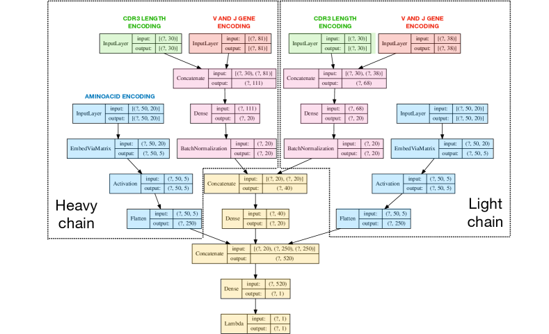
Figure S4: Neural Network structure of the deep-joint model for paired chains. See Fig. S1 for details on each layer.

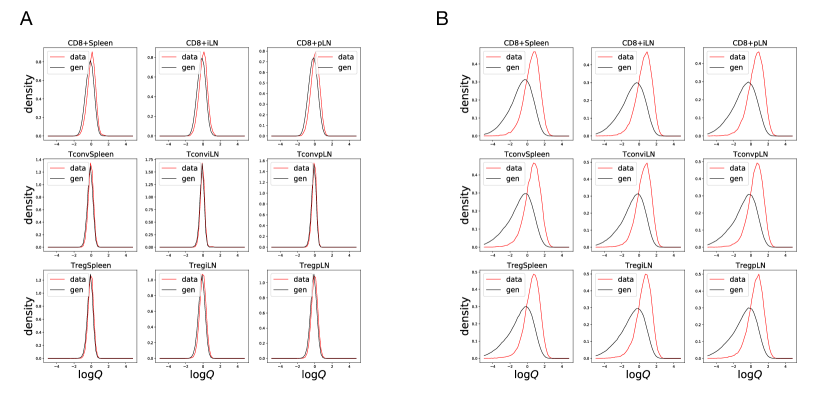
Figure S6: (A) Distribution of $\log\mathcal{Q}$ of inferred models starting from an empirical baseline ${\mathcal{G}}$, and (B) the distribution of $\log\mathcal{Q}$ of inferred models starting from the $P_{\rm gen}$ model as a baseline.

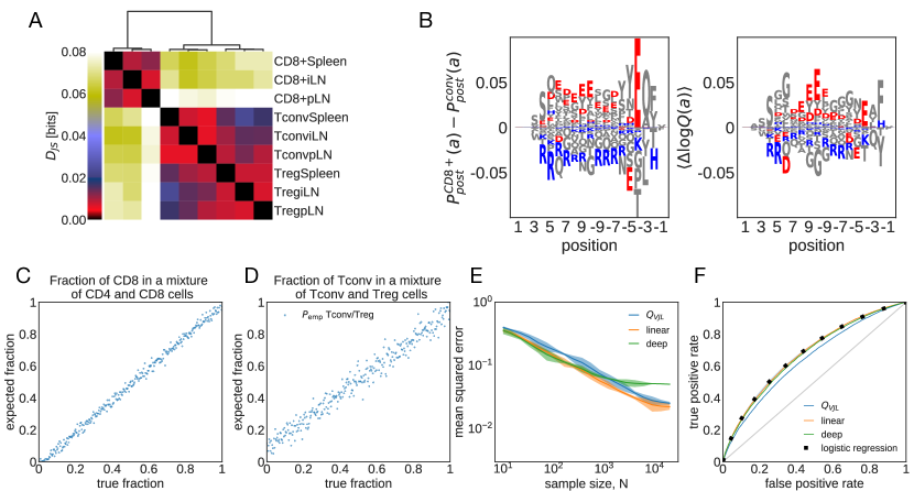
Figure S7: Analogous to Fig 4 in main text but with $P_{\rm gen}$ as null model. (A) Jensen-Shannon divergences ($D_{JS}$, see eq. 8 in Methods) computed from models trained on different sub-repertoires. (B) Difference in the marginal probability for amino acid composition along CDR3 between CD8⁺ and CD4⁺ Tconv (left) and the expected difference in the corresponding log-selection factors for amino acid usage (right) are shown. The negatively charged amino acids (Aspartate, D, and Glutamate, E) and the positively charged amino acids (Lysine, K, and Arginine, R) are indicated in red and blue, respectively. Other amino acids are shown in gray. (C) Maximum-likelihood inference of the fraction of CD8⁺ TCRs in mixed repertoires of Tconv and CD8⁺ cells from spleen (eq. 4). Each repertoires comprises $5\times 10^{3}$ unique TCR. (D) Same as (C) but for a mixture of Tconv and Treg TCR. (E) Mean squared error of the inferred sample fraction from (C) as a function of sample size $N$, averaged over all fractions, using models of increasing complexity: “$Q_{VJL}$” is a linear model with only features for CDR3 length and VJ usage, “linear” is linear SONIA model, ‘deep’ is the full soNNia model (see Fig. 1C). (F) Receiving-Operating Curve (ROC) for classifying individual sequences as coming from CD8⁺ cells or from CD4⁺ conventional T cells from spleen, using the log-likelihood ratios. Curves are generated by varying the threshold in eq. 5. The accuracy of the classifier is compared to a traditional logistic classifier inferred on the same set of features as our selection models. The training set for the logistic classifier has $N=3\times 10^{5}$ Tconv CD4⁺, $N=8.7\times 10^{4}$ CD8⁺ TCRs, and the test set has $N=2\times 10^{4}$ CD4, $N=2\times 10^{4}$ CD8⁺ TCR sequences.

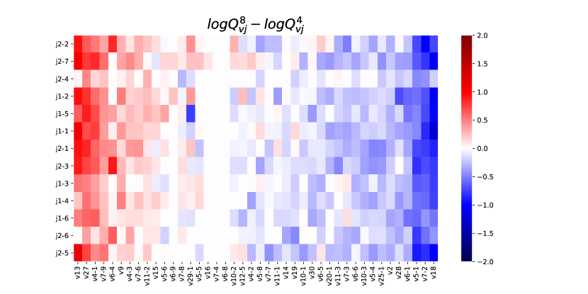
Figure S8: Differential selection on V and J gene usage between CD4⁺ and CD8⁺ models inferred on top of $P_{\rm emp}$ as baseline distribution.

Figure S10: (A-D) Parameters of generation models between CD4⁺ and CD8⁺ T cells do not differ significantly. (E,F) V and J gene usages in productive CD4⁺ Tconv and CD8⁺ T cells, for comparison to (A,B).

Figure S11: Joint Inference of fraction of (A) Treg and (B) CD4⁺ Tconv cells, belonging to different subclasses in a mixture of 3 repertoires: CD8⁺,CD4⁺ Tconv, and CD4⁺ Treg cells. We optimized the likelihood $L(f_{1},f_{2})=\sum_{i}(f_{1}Q_{\rm conv}(x_{i})+f_{2}Q_{\rm reg}(x_{i})+(1-f_{1}-f_{2})Q_{CD8}(x_{i}))$ to infer jointly the two fractions $f_{1}$ and $f_{2}$ in a chosen mixture of $3\times 10^{4}$ TCRs $x_{i}$, built by combining repertoires of purified subsets harvested from spleen [6]. Each point corresponds to a mixture with $f_{1}$ and $f_{2}$ sampled uniformly 2000 times in the simplex $f_{1}\geq 0$, $f_{2}\geq 0$, $f_{1}+f_{2}\leq 1$.

Figure S12: ROC curve between all subsets based on the log ratio $R(x)$ defined on main text, where the selection factors are inferred starting from the empirical baseline ${\mathcal{G}}$ ($P_{\rm emp}({\bf{x}})=N_{G}^{-1}\sum_{i=1}^{N_{G}}\delta_{{\bf{x}},x^{\prime}_{i}}$, above diagonal) or $P_{\rm gen}$ (below diagonal).

References

- [1] Emerson RO, et al. (2017) Immunosequencing identifies signatures of cytomegalovirus exposure history and HLA-mediated effects on the T cell repertoire Nat. Genet. 49:659–665.
- [2] Davidsen K, et al. (2019) Deep generative models for T cell receptor protein sequences eLife 8:e46935.
- [3] DeWitt WS, et al. (2018) Human T cell receptor occurrence patterns encode immune history, genetic background, and receptor specificity eLife 7:1–39.
- [4] Tanno H, et al. (2020) Determinants governing T cell receptor -chain pairing in repertoire formation of identical twins Proc. Natl. Acad. Sci. 117:532–540.
- [5] DeKosky BJ, et al. (2016) Large-scale sequence and structural comparisons of human naive and antigen-experienced antibody repertoires Proc. Natl. Acad. Sci. 113:E2636–E2645.
- [6] Seay HR, et al. (2016) Tissue distribution and clonal diversity of the T and B cell repertoire in type 1 diabetes JCI Insight 1:1–19.
- [7] Dean J, et al. (2015) Annotation of pseudogenic gene segments by massively parallel sequencing of rearranged lymphocyte receptor loci Genome Medicine 7:123.
- [8] Murugan A, Mora T, Walczak AM, Callan CG (2012) Statistical inference of the generation probability of T-cell receptors from sequence repertoires Proc. Natl. Acad. Sci. 109:16161–16166.
- [9] Marcou Q, Mora T, Walczak AM (2018) High-throughput immune repertoire analysis with IGoR Nat. Commun. 9:561.
- [10] Sethna Z, Elhanati Y, Callan CG, Walczak AM, Mora T (2019) OLGA: fast computation of generation probabilities of B- and T-cell receptor amino acid sequences and motifs Bioinformatics 35:2974–2981.
- [11] Sethna Z, et al. (2020) Population variability in the generation and selection of T-cell repertoires PLOS Comput. Biol. 16:e1008394.
- [12] Ioffe S, Szegedy C (2015) Batch Normalization: Accelerating Deep Network Training by Reducing Internal Covariate Shift CoRR abs/1502.03167.
- [13] Chollet F, et al. (2015) Keras (https://keras.io).
- [14] Elhanati Y, Murugan A, Callan CG, Mora T, Walczak AM (2014) Quantifying selection in immune receptor repertoires Proc. Natl. Acad. Sci. 111:9875–9880.
- [15] Emerson R, et al. (2013) Estimating the ratio of CD4+ to CD8+ T cells using high-throughput sequence data J. Immunol. Methods 391:14 – 21.
- [16] Steuer R, Kurths J, Daub CO, Weise J, Selbig J (2002) The mutual information: Detecting and evaluating dependencies between variables Bioinformatics 18:S231–S240.