Bias correction for quantile regression estimators

Abstract

We study the bias of classical quantile regression and instrumental variable quantile regression estimators. While being asymptotically first-order unbiased, these estimators can have non-negligible second-order biases. We derive a higher-order stochastic expansion of these estimators using empirical process theory. Based on this expansion, we derive an explicit formula for the second-order bias and propose a feasible bias correction procedure that uses finite-difference estimators of the bias components. The proposed bias correction method performs well in simulations. We provide an empirical illustration using Engel’s classical data on household expenditure.

JEL Classification: C21, C26.

Keywords: instrumental variables, higher-order stochastic expansion, Bahadur-Kiefer expansion, finite-difference estimators, mixed integer linear programming (MILP).

1 Introduction

Many interesting empirical applications of classical quantile regression (QR) (Koenker and Bassett, 1978) and instrumental variable quantile regression (IVQR) (Chernozhukov and Hansen, 2005, 2006) feature small sample sizes, which can arise either as a result of a limited number of observations or when estimating tail quantiles, or both (e.g., Chernozhukov, 2005; Elsner et al., 2008; Chernozhukov and Fernández-Val, 2011; Adrian and Brunnermeier, 2016; Adrian et al., 2019). QR and IVQR estimators are nonlinear and can thus exhibit substantial biases in small samples. In this paper, we theoretically characterize these biases and develop a feasible bias correction procedure.

To study the biases, we start by deriving a higher-order stochastic expansion of the classical QR and exact IVQR estimators. Such an expansion is needed because the higher-order terms contribute nonzero biases while the first-order term does not. We derive explicit expressions and uniform (in the quantile level) rates for the components in the expansion, building on the empirical process arguments of Ota et al. (2019). This expansion can be thought of as a refined Bahadur-Kiefer (BK) representation of the estimator that decomposes the nonlinear component into terms up to the order $O_{p}\left(n^{-1}\right)$ and a $O_{p}\left(n^{-5/4}\sqrt{\log n}\right)$ remainder.

Using the stochastic expansion, we study the bias of QR and exact IVQR estimators. We derive a bias formula based on the leading terms up to order $O_{p}\left(n^{-1}\right)$ in the expansion, which we refer to as the second-order (asymptotic) bias. This approach of focusing on the moments of the leading terms in the stochastic expansions is standard in the literature. The second-order bias formula provides an approximation of the actual bias that yields a feasible correction. Our results explicitly account for the $O\left(n^{-1}\right)$ (up to a logarithmic factor) bias due to nonzero sample moments at the estimator. Our proof strategy is different from the generalized function heuristic used in the existing literature (Phillips, 1991; Lee et al., 2017, 2018), which does not account for all the leading terms up to $O\left(n^{-1}\right)$ in the bias. The missing terms can be important bias contributors in practice, as we document in the empirical application in Section 5.

A feasible bias correction procedure then follows from the second-order bias formula. We propose finite-difference estimators of all the components in the formula. These estimators admit higher-order expansions that allow us to select bandwidth rates. We show that the resulting bias-corrected estimator has zero second-order bias.

We evaluate the performance of our bias correction procedure in a Monte Carlo simulation study. The simulations show that the theoretical (infeasible) bias formula describes well the second-order bias of classical QR and exact IVQR. We find that the proposed feasible bias correction can effectively reduce the bias in many cases, even in samples as small as $n=50$. However, strong asymmetry and, especially, heavy tails in the conditional distribution of the outcome may reduce the effectiveness of bias correction. The impact of the feasible bias correction on the root MSE (RMSE) is rather small and ambiguous.

We illustrate the bias correction approach by revisiting the relationship between food expenditure and income based on the original Engel (1857) data (e.g., Koenker and Bassett, 1982; Koenker and Hallock, 2001). Our results highlight the importance of bias correction in empirical applications with small sample sizes. Specifically, we find that the second-order bias of classical QR is non-negligible, especially at the upper tail, leading QR to underestimate the effect heterogeneity across quantiles.

Roadmap.

The remainder of the paper is organized as follows. Section 2 describes the model and the estimators. Section 3 provides our main theoretical results. Section 4 presents the Monte Carlo simulation results. Section 5 contains the empirical application. Section 6 concludes. All the proofs and some additional details are given in the Appendix.

2 Model and estimators

Consider a setting with a continuous outcome variable $Y$, a $(k\times 1)$ vector of covariates $W$, and a $(k\times 1)$ vector of instruments $Z$. We assume throughout that $k$ is fixed. Every observation $(Y_{i},W_{i},Z_{i})$, $i=1,\dots,n$, is jointly drawn from a distribution $P$. We assume that $(Y_{i},W_{i},Z_{i})$ is i.i.d., and we will sometimes suppress the index $i$ to lighten up the notation. The parameter of interest $\theta_{\tau}\in\Theta\subset\mathbb{R}^{k}$ is defined as a solution to the following unconditional quantile moment restrictions,

$$\mathbb{E}[(1\{Y\leq W^{\prime}\theta_{\tau}\}-\tau)Z]=0,\quad\tau\in(0,1).$$ (1)

We consider two cases: (i) classical QR, where $Z=W$ (Koenker and Bassett, 1978), and (ii) linear IVQR, where $Z\neq W$ in general (Chernozhukov and Hansen, 2006, 2008).

The classical QR estimator of $\theta_{\tau}$ is a solution to the following convex minimization problem,

$$\hat{\theta}_{\tau,QR}\in\operatorname{argmin}_{\theta\in\Theta}\mathbb{E}_{n}\rho_{\tau}(Y-W^{\prime}\theta),$$ (2)

where $\rho_{\tau}(u)=u(\tau-1\{u<0\})$ is the check function (Koenker, 2005) and $\mathbb{E}_{n}$ denotes the sample average, i.e., the expectation with respect to the empirical measure. For IVQR, we consider estimators that exactly minimize the $p$-norm of the sample moments,

$$\hat{\theta}_{\tau,p}\in\operatorname{argmin}_{\theta\in\Theta}||\hat{g}_{\tau}(\theta)||_{p},$$ (3)

where $p\in[1,\infty]$ and $\hat{g}_{\tau}(\theta)\triangleq\mathbb{E}_{n}(1\{Y\leq W^{\prime}\theta\}-\tau)Z$. This class of exact IVQR estimators includes GMM, which corresponds to $p=2$ as in Chen and Lee (2018) for just-identified models, and the estimator proposed by Zhu (2019), which corresponds to $p=\infty$. The cases $p=1$ and $p=\infty$ have computationally convenient mixed integer linear programming (MILP) representations, while the MILP formulation for $p=2$ has many more decision variables. In our Monte Carlo simulations, we use $p=1$ for computational convenience (see Appendix D).

We use the notation $g_{\tau}(\theta)\triangleq\mathbb{E}(1\{Y\leq W^{\prime}\theta\}-\tau)Z$ for the unconditional moment restrictions as a function of $\theta\in\Theta$, and write $G(\theta)\triangleq\partial_{\theta}\mathbb{E}Z1\{Y\leq W^{\prime}\theta\}=\partial_{\theta}g_{\tau}(\theta)$ for its derivative. We maintain the following standard identification assumptions.

Assumption 1 (Identification).

1. $\theta_{\tau}$ is the unique solution to $g_{\tau}(\theta)=0$ over a compact set $\Theta\subset\mathbb{R}^{k}$, and $\theta_{\tau}$ is in the interior of $\Theta$ for all $\tau\in[\varepsilon,1-\varepsilon]$ for some $\varepsilon>0$.

2. The Jacobian $G(\theta_{\tau})$ has full rank for all $\tau\in(0,1)$.

As noted by Chernozhukov and Hansen (2006, p.502), compactness of the parameter space $\Theta$ “is not restrictive in micro-econometric applications.” Throughout the paper, we use the short notation $G$ for $G(\theta_{\tau})$ whenever it does not lead to ambiguity.

We impose the following smoothness assumptions on the conditional density and its derivatives. Such assumptions are standard in the literature on higher-order properties of quantile estimators (e.g., Ota et al., 2019).

Assumption 2 (Conditional density).

The conditional density of $Y_{i}$ given $(W_{i},Z_{i})$, $f_{Y}(y|w,z)$, exists, is a.s. three times continuously differentiable on $supp(Y)$, and there exists a constant $\bar{f}$ such that $|f^{(r)}_{Y}(y|w,z)|\leq\bar{f}$ for all $(y,w,z)\in supp(Y)\times supp(W)\times supp(Z)$, where $r=0,1$ and $f_{Y}^{(r)}(\cdot|w,z)$ is the $r$-th derivative of $f_{Y}(\cdot|w,z)$.

In our theoretical analysis of the bias, we will often work with a related object, the conditional density $f_{\varepsilon_{\tau}}(e|W,Z)\triangleq f_{Y}(e+W^{\prime}\theta_{\tau}|W,Z)$ of the quantile residual $\varepsilon_{\tau}\triangleq Y-W^{\prime}\theta_{\tau}$.

Finally, we assume that the regressors and the instruments have bounded higher-order moments.

Assumption 3 (Regressors and instruments).

There exists constants $m<\infty$ and $\gamma\geq 6$ such that $\mathbb{E}|W_{j}|^{\gamma}\leq m$ and $\mathbb{E}|Z_{j}|^{\gamma}\leq m$ for all $j=1,\dots,k$.

Assumption 3 guarantees the existence of all relevant moments of the terms involving $W$ and $Z$ in the higher-order derivatives of the moment conditions and the bias correction (e.g., $\mathbb{E}Z_{\ell}W_{j}W_{q}W_{r}$). The power parameter $\gamma$ (as we show below) determines the upper bound on the rate at which the norm of the sample moment functions converge to zero — higher $\gamma$ implies faster convergence to zero.

3 Asymptotic theory for bias correction

To derive a bias correction procedure, we follow the approach of Nagar (1959) and focus on the bias of the leading terms in an asymptotic stochastic expansion of the estimator.

3.1 Stochastic expansion of quantile regression estimators

The classical first-order asymptotic theory for quantile regression estimators (e.g., Koenker and Bassett, 1978; Angrist et al., 2006; Chernozhukov and Hansen, 2006; Kaplan and Sun, 2017; Kaido and Wüthrich, 2021) is based on the following leading term,

$$\hat{\xi}_{\tau}\triangleq\theta_{\tau}-G^{-1}(\theta_{\tau})\mathbb{E}_{n}Z\left(1\{Y\leq W^{\prime}\theta_{\tau}\}-\tau\right).$$ (4)

For correctly specified models, $\hat{\xi}_{\tau}$ is an infeasible unbiased estimator of $\theta_{\tau}$. However, because feasible quantile estimators are nonlinear, they generally have a nonzero higher-order bias. The following theorem provides a characterization of the terms in a stochastic expansion of $\hat{\theta}_{\tau}$ up to order $O_{p}\left(n^{-1}\right)$ (ignoring logarithmic terms).

To state the result, we introduce some additional notation. For $\theta\in\Theta$, define the auxiliary functions $g^{\circ}(\theta)\triangleq\mathbb{E}1\{Y\leq W^{\prime}\theta\}Z$, $B^{\circ}_{n}(\theta)\triangleq\sqrt{n}(\mathbb{E}_{n}1\{Y\leq W^{\prime}\theta\}Z-g^{\circ}(\theta))$, and $B_{n}(\theta)\triangleq B^{\circ}_{n}(\theta)-B^{\circ}_{n}(\theta_{\tau})$. Also, denote the Hessian of the $j$-th moment function $g_{j}$ by $\partial_{\theta}G_{j}(\theta)\triangleq\partial_{\theta}\partial_{\theta}g_{j}(\theta)$. Finally, for any $x\in\mathbb{R}^{k}$, denote by $x^{\prime}\partial_{\theta}G(\theta)x$ the vector with components $x^{\prime}\partial_{\theta}G_{j}(\theta)x$, $j=1,\dots,k$.

Theorem 1.

Suppose that Assumptions 1–3 hold. Consider $\hat{\theta}_{\tau}=\hat{\theta}_{\tau,p}$ obtained from program (3) for some $p\in[1,\infty]$ or $\hat{\theta}_{\tau}=\hat{\theta}_{\tau,QR}$. Then

$$\hat{\theta}_{\tau}=\hat{\xi}_{\tau}+G^{-1}(\theta_{\tau})\left[\hat{g}_{\tau}(\hat{\theta}_{\tau})-\frac{B_{n}(\hat{\theta}_{\tau})}{\sqrt{n}}-\frac{1}{2}(\hat{\xi}_{\tau}-\theta_{\tau})^{\prime}\partial_{\theta}G(\theta_{\tau})(\hat{\xi}_{\tau}-\theta_{\tau})\right]+R_{n,\tau},$$

where

$$\sup_{\tau\in[\varepsilon,1-\varepsilon]}\|\hat{g}_{\tau}(\hat{\theta}_{\tau})\| =\begin{cases}O_{p}\left(\frac{1}{n}\right),\text{ if }\hat{\theta}_{\tau}=\hat{\theta}_{\tau,\text{QR}},\\ O_{p}\left(\frac{\log n}{n^{1-\frac{2}{\gamma}}}\right),\text{ if }\hat{\theta}_{\tau}=\hat{\theta}_{\tau,p},\end{cases}$$ (5)

$$\sup_{\tau\in[\varepsilon,1-\varepsilon]}\|B_{n}(\hat{\theta}_{\tau})\| =O_{p}\left(\frac{\sqrt{\log n}}{n^{1/4}}\right),$$ (6)

$$\sup_{\tau\in[\varepsilon,1-\varepsilon]}\|\hat{\xi}_{\tau}-\theta_{\tau}\| =O_{p}\left(\frac{1}{n^{1/2}}\right),$$ (7)

$$\sup_{\tau\in[\varepsilon,1-\varepsilon]}\|R_{n,\tau}\| =O_{p}\left(\frac{\sqrt{\log n}}{n^{5/4}}\right).$$

The proof of Theorem 1 builds on the empirical process arguments in Lemma 3 of Ota et al. (2019) and uses the maximal inequality in Corollary 5.1 of Chernozhukov et al. (2014).

The rates in Theorem 1 are uniform in the quantile level $\tau$. Uniformity is important in theory and practice because QR and IVQR methods are particularly powerful when used to analyze the entire quantile process.

Classical QR and linear IVQR are motivated by the linearity of the true conditional quantile function. In practice, linearity may be restrictive, especially when it is imposed at each $\tau\in(0,1)$. While the result in Theorem 1 remains valid if linearity fails, the interpretation is more complicated in this case. Specifically, if the true conditional quantiles are nonlinear, then the expansion in Theorem 1 applies to the pseudo-true value defined via moment condition (1). For classical QR, this pseudo-true value can be interpreted as the minimizer of a weighted mean-squared error loss function (Angrist et al., 2006). Note further that the result in Theorem 1 holds for every fixed $\tau\in(0,1)$. Thus, if linearity holds at a given $\tau$, we can interpret the expansion at this $\tau$ under the correct specification without requiring linearity at the other quantile levels.

The expansion in Theorem 1 can be thought of as a refined Bahadur-Kiefer (BK) expansion. Different from standard BK expansions, we do not bundle together all the higher-order terms (as opposed to, for example, Zhou and Portnoy, 1996; Ota et al., 2019). Notice that the dominant nonlinear term in the BK expansion, $n^{-1/2}G^{-1}B_{n}(\hat{\theta}_{\tau})$, has order $O_{p}\left(n^{-3/4}\sqrt{\log n}\right)$ (Equation (6)). Theorem 3 in Knight (2002) shows that for classical QR with discrete covariates, this term converges in distribution to a zero mean random process. Therefore, we explicitly extract the higher-order terms up to order $O_{p}\left(n^{-1}\right)$ (ignoring logarithmic terms) from the BK remainder. As we will show in the following sections, these higher-order terms admit feasible counterparts.

Remark 1 (Alternative approach for deriving stochastic expansions).

Portnoy (2012) proposed an alternative approach for deriving a stochastic expansion of classical QR estimators. This approach yields bounds on the precision of a nonlinear Gaussian approximation of order $O_{p}\left(n^{-1}\log^{5/2}n\right)$. As we will show, the expansion in Theorem 1 yields a bias formula for both QR and IVQR estimators that admits a feasible implementation. The results in Portnoy (2012) are specific to classical QR, and it is not clear to us whether these results can be used for bias correction using a Nagar-style approach. ∎

Remark 2 (General IVQR estimators).

While we focus on exact IVQR estimators in the main text, the results in Theorem 1 can be used to obtain a uniform BK expansion for general 1-step corrected IVQR estimators. See Appendix E for details. ∎

3.2 Bias formula for exact estimators

Following common practice (e.g., Nagar, 1959; Kaplan and Sun, 2017), for a generic estimator $\hat{\gamma}$, we define the second-order bias $\operatorname{Bias}(\hat{\gamma})$ as the bias of the leading terms in the stochastic expansion of $\hat{\gamma}$ up to the order $O_{p}\left(n^{-1}\right)$. This second-order bias can be interpreted as an approximation of the actual bias that works with arbitrarily high probability in large samples.

Before stating the result, we observe that under our Assumption 2, the moment condition (1) is equivalent to

$$\mathbb{E}[(1\{-Y\leq W^{\prime}(-\theta_{\tau})\}-(1-\tau))Z]=0.$$

Thus, we can characterize the QR and IVQR estimators using the moment function $g_{\tau}^{*}(\theta)\triangleq\mathbb{E}[(1\{-Y\leq W^{\prime}\theta\}-(1-\tau))Z]$ with sample analog $\hat{g}_{\tau}^{\ast}(\theta)$. The following theorem characterizes the second-order bias in terms of $\hat{g}_{\tau}(\hat{\theta})$ and $\hat{g}_{\tau}^{*}(-\hat{\theta})$. As in Section 3.1, we define $\partial_{\theta}G_{j}(\theta)\triangleq\partial_{\theta}\partial_{\theta}g_{j}(\theta)$ for all $\theta\in\Theta$.

Theorem 2.

Suppose that Assumptions 1–3 hold. Consider $\hat{\theta}_{\tau}=\hat{\theta}_{\tau,p}$ obtained from program (3) for some $p\in[1,\infty]$ or $\hat{\theta}_{\tau}=\hat{\theta}_{\tau,QR}$. Then the second-order bias is

$$\operatorname{Bias}(\hat{\theta}_{\tau})=G^{-1}(\theta_{\tau})\left[\frac{1}{2}\mathbb{E}\left(\hat{g}_{\tau}(\hat{\theta}_{\tau})-\hat{g}_{\tau}^{*}(-\hat{\theta}_{\tau})\right)-\frac{\kappa_{\tau}}{n}-\frac{1}{2n}Q^{\prime}vec(\Omega_{\tau})\right],$$ (8)

where

$$\kappa_{\tau} \triangleq\left(\tau-\frac{1}{2}\right)\mathbb{E}f_{\varepsilon_{\tau}}(0|W,Z)ZW^{\prime}G^{-1}Z,$$

$$\Omega_{\tau} \triangleq\operatorname{Var}[Z(1\{Y\leq W^{\prime}\theta_{\tau}\}-\tau)],$$

$$Q \text{ is a matrix with columns }Q_{j}\triangleq\operatorname{vec}\left[(G^{-1})^{\prime}\partial_{\theta}G_{j}(\theta_{\tau})G^{-1}\right],\,\,j=1,\dots,k.$$

The second-order bias formula (8) has three components.

The first component, $G^{-1}\mathbb{E}\left(\hat{g}_{\tau}(\hat{\theta}_{\tau})-\hat{g}_{\tau}^{*}(-\hat{\theta}_{\tau})\right)/2$, captures the bias from the sample moments not being zero at the estimator. This term is not equal to zero in general. By Theorem 1 and Assumption 3, this term has bias of order at most $O\left(n^{-1+2/\gamma}\log n\right)$.

The second component, $n^{-1}G^{-1}\kappa_{\tau}$, appears because of the discontinuity in the sample moment functions. The term $\kappa_{\tau}$ reflects the dependence between the sample moments and the linear influence of a single observation on $\hat{\theta}_{\tau}$. Notice that the first two components combined correspond to the second order bias of the terms $G^{-1}(\theta_{\tau})(\hat{g}_{\tau}(\hat{\theta}_{\tau})-n^{-1/2}B_{n}(\hat{\theta}_{\tau}))$ in Theorem 1.

The last component, $(2n)^{-1}G^{-1}Q^{\prime}vec(\Omega)$, stems from the non-uniformity of the conditional distribution of $Y$ given $(W,Z)$. This term correspond to the term $G^{-1}(\theta_{\tau})(\hat{\xi}_{\tau}-\theta_{\tau})^{\prime}\partial_{\theta}G(\theta_{\tau})(\hat{\xi}_{\tau}-\theta_{\tau})/2$ in Theorem 1. Similar terms are typically present in most nonlinear estimators with nonzero Hessian of the score function (see, for example, Rilstone et al., 1996).

To illustrate the approximate bias formula, consider an order statistic of $Y\sim\text{Uniform}(0,1)$ (corresponding to our framework with $Z=W=1$), for which an exact bias formula is available (e.g., Ahsanullah et al., 2013). We show in Appendix C that the precision of the second-order bias formula in this case is $O\left(n^{-2}\right)$, which is smaller than the order of the remainder term in the stochastic expansion of Theorem 1. Figure 1 illustrates the precision of the asymptotic formula by comparing it to the actual bias of the order statistic.

Figure 1: Exact (circles) and second-order (crosses) biases, scaled by $n$, as functions of quantile level $\tau$ for $\hat{\theta}_{\tau}=Y_{(\lfloor\tau n\rfloor)}$, where $Y\sim\text{Uniform}(0,1)$, $n=10$.

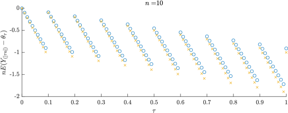
It is interesting to compare our results to the higher-order bias analysis of non-smooth estimators based on the generalized functions heuristic (e.g., Phillips, 1991). In recent work, Lee et al. (2017, 2018) derived a second-order bias formula for classical QR and IVQR under the assumption that the sample moments are zero at the estimator so that the first term of the bias formula vanishes. We show in Appendix C that this term is non-negligible even in simple cases (see also Figure 5 in Section 5).

3.3 Feasible bias correction

The bias formula suggests the following feasible bias-corrected estimator,

$$\hat{\theta}_{bc}=\hat{\theta}_{\tau}-\frac{1}{2}\hat{G}^{-1}\left[\hat{g}_{\tau}(\hat{\theta}_{\tau})-\hat{g}_{\tau}^{*}(-\hat{\theta}_{\tau})\right]+\frac{1}{n}\hat{G}^{-1}\left[\hat{\kappa}_{\tau}+\frac{1}{2}\hat{Q}^{\prime}vec(\hat{\Omega})\right],$$

where $\hat{G}$, $\hat{\kappa}_{\tau}$, $\hat{Q}$, and $\hat{\Omega}$ are estimators of $G$, $\kappa_{\tau}$, $Q$, and $\Omega$, respectively, satisfying the following consistency requirement.

Assumption 4 (Consistency of component estimators).

The estimators $\hat{G}$, $\hat{\kappa}_{\tau}$, $\hat{Q}$, and $\hat{\Omega}$ are consistent for $G$, $\kappa_{\tau}$, $Q$, and $\Omega$, respectively. Moreover, $\hat{G}-G=o_{p}\left((n^{1/3}\log n)^{-1}\right)$.

In Section 3.4, we propose finite-difference estimators for which Assumption 4 holds under Assumptions 1–3. Assumption 4 could also be verified for other nonparametric estimators of the bias components.

The next theorem shows that the second-order bias of the bias-corrected estimator is zero.

Theorem 3.

Suppose that Assumptions 1–4 hold. Consider $\hat{\theta}_{\tau}=\hat{\theta}_{\tau,p}$ obtained from program (3) for some $p\in[1,\infty]$ or $\hat{\theta}_{\tau}=\hat{\theta}_{\tau,QR}$. Then the bias correction eliminates the second-order bias, $\operatorname{Bias}\left(\hat{\theta}_{bc}\right)=0.$

Note that the requirement that $\hat{G}-G=o_{p}\left((n^{1/3}\log n)^{-1}\right)$ in Assumption 4 is necessary to ensure that the contribution of the product of the sample moments, which are $O_{p}\left(n^{-1+2/\gamma}\log n\right)$ with $\gamma\geq 6$ (as required by Assumption 3) by Theorem 1, and the estimation error in $G^{-1}$ can be omitted in computing the second-order bias. This condition is only required for IVQR estimators. For classical QR estimators, the sample moments are of order $O_{p}\left(n^{-1}\right)$, so that consistency of $\hat{G}$ at any rate of convergence suffices for Theorem 3.

3.4 Finite difference estimators of bias components

To implement the bias correction, we need estimators of $G$, $\kappa_{\tau}$, $Q$, and $\Omega$ that satisfy Assumption 4. The variance matrix $\Omega$ can be estimated using the analogy principle,

$$\hat{\Omega}_{\tau}\triangleq\mathbb{E}_{n}[Z(1\{Y\leq W^{\prime}\hat{\theta}_{\tau}\}-\tau)-\mathbb{E}_{n}Z(1\{Y\leq W^{\prime}\hat{\theta}_{\tau}\}-\tau)]^{2}.$$

All other bias components take the form of derivatives. Therefore, we leverage our theoretical results on the properties of the sample moments to develop a unified finite-difference framework for estimating these components.

Under Assumptions 1 and 2, the Jacobian is $G=\mathbb{E}f_{\varepsilon_{\tau}}(0|W,Z)ZW^{\prime}$ and the Hessian consists of gradients of the components of $G$, i.e. $\partial_{\theta}G_{i,j}(\theta_{\tau})=\mathbb{E}f^{(1)}_{\varepsilon_{\tau}}(0|W,Z)Z_{i}W_{j}W$, where $i,j=1,\dots,k.$ This suggests the following analog estimators.

The $(i,j)$-th component of $G$ can be estimated using Powell (1986)’s estimator

$$\hat{G}_{i,j}=\mathbb{E}_{n}\left[\frac{1\{Y\leq W^{\prime}\hat{\theta}_{\tau}+h_{1,n}\}-1\{Y\leq W^{\prime}\hat{\theta}_{\tau}-h_{1,n}\}}{2h_{1,n}}Z_{i}W_{j}\right],$$ (9)

where $h_{1,n}\to 0$ is a bandwidth. Denote by $e_{\ell}$ the $\ell$-th unit vector in $\mathbb{R}^{k}$, where $\ell=1,\dots,k$. The derivative of the $(i,j)$-th component of $G$ in the direction $e_{\ell}$ (i.e. the second partial derivative of $g_{\tau}$) can be estimated as the symmetric first difference of (9),

$$\widehat{({\partial_{\theta}G}_{i,j})}_{\ell} =\mathbb{E}_{n}\left[\frac{1\{Y\leq W^{\prime}\hat{\theta}_{\tau}+h_{2,n}\}-2\cdot 1\{Y\leq W^{\prime}\hat{\theta}_{\tau}\}+1\{Y\leq W^{\prime}\hat{\theta}_{\tau}-h_{2,n}\}}{h_{2,n}^{2}}Z_{i}W_{j}W_{\ell}\right],$$

where $h_{2,n}\to 0$ is a (potentially different) bandwidth. For $\kappa_{\tau}$, the finite difference sample analog is

$$\hat{\kappa}_{\tau}=\left(\tau-\frac{1}{2}\right)\mathbb{E}_{n}\left[\frac{1\{Y\leq W^{\prime}\hat{\theta}_{\tau}+h_{3,n}\}-1\{Y\leq W^{\prime}\hat{\theta}_{\tau}-h_{3,n}\}}{2h_{3,n}}ZW^{\prime}\hat{G}^{-1}Z\right],$$

where $h_{3,n}\to 0$ is a bandwidth. Finally, $Q$ can be estimated by the sample analog matrix $\hat{Q}$ with columns

$$\hat{Q}_{j}\triangleq vec\left[(\hat{G}^{-1})^{\prime}\widehat{\partial_{\theta}G_{j}}\hat{G}^{-1}\right],\quad j=1,\dots,k,$$

where $\widehat{\partial_{\theta}G_{j}}$ is the matrix with elements $\widehat{({\partial_{\theta}G}_{i,j})}_{\ell}$ for $i,\ell=1,\dots,k$.

The next lemma establishes the consistency of the estimators of the bias components. It implies that these estimators satisfy the high-level conditions in Assumption 4. Moreover, it provides nearly remainder-optimal bandwidth rates, i.e., the rates that yield the fastest convergence rates of the stochastic remainder terms of the corresponding stochastic expansions (up to logarithmic terms).

Lemma 1.

Suppose that Assumptions 1–3 hold. Then the nearly remainder-optimal bandwidth rates are $h_{1,n}\propto n^{-1/5}$, $h_{2,n}\propto n^{-1/7}$, $h_{3,n}\propto n^{-2/15}$, and, under these bandwidth rates,

$$\hat{G} =G+O_{p}\left(\frac{\sqrt{\log n}}{n^{2/5}}\right),$$

$$\widehat{({\partial_{\theta}G}_{i,j})}_{\ell} ={({\partial_{\theta}G}_{i,j})}_{\ell}+O_{p}\left(\frac{\sqrt{\log n}}{n^{2/7}}\right),$$

$$\hat{Q}_{j} =Q_{j}+O_{p}\left(\frac{\sqrt{\log n}}{n^{2/7}}\right),$$

$$\hat{\kappa}_{\tau} =\kappa_{\tau}+O_{p}\left(\frac{\sqrt{\log n}}{n^{4/15}}\right),$$

$$\hat{\Omega}_{\tau} =\Omega+O_{p}\left(\frac{1}{\sqrt{n}}\right).$$

Moreover, the convergence rate for $\hat{G}$ is uniform in $\tau\in[\varepsilon,1-\varepsilon]$.

Proposition 1 in Kato (2012) shows that the remainder rate for $\hat{G}$ in Lemma 1, $h_{1,n}\propto n^{-1/5}$, is the AMSE-optimal rate. To implement the finite difference estimators in practice, one needs to choose constants in addition to the bandwidth rates. We discuss the choice of these constants in Sections 4 and 5.

4 Simulation evidence

In this section, we evaluate the performance of our feasible bias correction procedure in a Monte Carlo simulation study. We consider data-generating processes (DGPs) inspired by the simulations in Andrews and Mikusheva (2016). The outcome is generated according to the following location-scale model

$$Y_{i}=W_{i}+(0.5+W_{i})U_{i},\quad i=1,\dots,n,$$

where $W_{i}=\Phi(\tilde{W}_{i})$, $Z_{i}=\Phi(\tilde{Z}_{i})$, $U_{i}=F_{U}^{-1}\left(\Phi(\tilde{U}_{i})\right)$, $(\tilde{W}_{i},\tilde{Z}_{i},\tilde{U}_{i})\sim N(0,\Sigma)$, $\Sigma_{11}=\Sigma_{22}=\Sigma_{33}=1$, $\Sigma_{23}=0$, and $\Phi$ is the standard normal CDF. Hence, in all the designs, both the regressors and the instruments are $\operatorname{Uniform}[0,1]$. We consider four DGPs that differ with respect to the error distribution $F_{U}$ and whether or not $W$ is exogenous.

DGP1 (Uniform, exogenous)	$F_{U}(u)=\int_{-\infty}^{u}1\{t\in[0,1]\}dt$	$\Sigma_{12}=1$, $\Sigma_{13}=0$
DGP2 (Triangular, exogenous)	$F_{U}(u)=\int_{-\infty}^{u}2t1\{t\in[0,1]\}dt$	$\Sigma_{12}=1$, $\Sigma_{13}=0$
DGP3 (Cauchy, exogenous)	$F_{U}(u)=\int_{-\infty}^{u}\frac{1}{\pi(1+(4t)^{2})}dt$	$\Sigma_{12}=1$, $\Sigma_{13}=0$
DGP4 (Uniform, endogenous)	$F_{U}(u)=\int_{-\infty}^{u}1\{t\in[0,1]\}dt$	$\Sigma_{12}=0.75$, $\Sigma_{13}=0.25$

An important practical issue is the choice of the bandwidths $h_{1,n}$, $h_{2,n}$, and $h_{3,n}$. We choose the nearly remainder-optimal rates for the bandwidths from Lemma 1: $h_{1,n}=A_{G}n^{-1/5}$, $h_{2,n}=A_{Q}n^{-1/7}$, $h_{3,n}=A_{\kappa}n^{-2/15}$, where $(A_{G},A_{Q},A_{\kappa})$ are constants that are independent of the sample size. We report results for both our baseline choice $(A_{G},A_{Q},A_{\kappa})=(1,1,1)$ and the choice of $(A_{G},A_{Q},A_{\kappa})$ that minimizes the $\ell_{2}$-distance between the residual biases after infeasible and feasible correction for the intercept and the slope parameter over the grid

$$\mathcal{A}\triangleq\{(1,1,1),(1.5,1,1),(0.5,1,1),(1,1.5,1),(1,0.5,1),(1,1,1.5),(1,1,0.5)\}.$$ (10)

Figure 6 in Appendix F shows how the results change if we increase/decrease each element of $(A_{G},A_{Q},A_{\kappa})$, one at a time.

We focus on the performance of bias correction for $\tau\in\{0.25,0.5,0.75\}$. To evaluate the precision of the Monte Carlo integration, we compute the Monte Carlo standard error (MCSE). We report $\Phi^{-1}(1-0.05/12)\times$ MCSE to account for the joint testing of six hypotheses (two hypotheses per each of three levels of $\tau$). For comparison, we also display the infeasible bias correction based on the true $G$, $Q$, and $\kappa$.

Figure 2 shows the results for the exogenous DGP1 with $n\in\{50,100,200\}$ based on classical QR of $Y$ on $W$, implemented via linear programming (see Appendix D). Notice that the scaled bias of the QR estimator, $n(\mathbb{E}\hat{\theta}_{\tau,\text{QR}}-\theta_{\tau})$, (blue dots) has the same range across the different sample sizes. This illustrates that we are estimating $O(n^{-1})$ terms in the asymptotic bias expansion, which should be approximately constant after scaling by $n$. One can see that the infeasible bias correction (gold dashed lines) reduces the bias at most quantile levels. The correction does not result in zero bias due to the finite precision of the simulation (the sample moment term does not have an explicit bias formula) and the presence of the higher-order bias terms. Notice that the MCSE grows with the sample size for a fixed number of simulations due to the rescaling, which helps explain the seemingly better performance for $n=50$.

We find that the feasible bias correction (gold squares and crosses) typically reduces the bias at $\tau\in\{0.25,0.75\}$, where the bias of classical QR is largest, and can get very close to the infeasible bias correction. At $\tau=0.5$, the bias of classical QR is small so that the feasible bias correction has a negligible impact. The feasible bias correction with the baseline bandwidth choice $(1,1,1)$ results in comparable deviations from the infeasible one across the different sample sizes. This is consistent with Lemma 1 since, otherwise, different sample sizes would require different constants $A_{G},A_{Q},A_{\kappa}$.

In Figure 3, we study the role of the error distribution $F_{U}$ and endogeneity. The infeasible bias correction reduces the bias across all the DGPs. Panels (a) and (b) document two cases that present challenges for the feasible bias correction procedure in small samples: strong asymmetry in DGP2, which may affect the performance at the median, and, especially, heavy tails in DGP3, which may affect the performance at tail quantiles. Panel (c) demonstrates that the bias correction performs well when combined with IVQR implemented using the MILP formulation in Appendix D. While the scaled second-order bias of IVQR can be substantial, especially for the slope parameter, the feasible bias correction effectively reduces that bias across all quantile levels considered.

We investigate the impact of bias correction on the RMSE of the estimators in Figure 4. We report the results for QR based on the exogenous DGP1 and IVQR based on the endogenous DGP4 with $n=100$. Overall, the impact of bias correction on the RMSE is small. While it slightly increases the RMSE for DGP1, it sometimes decreases the RMSE for DGP4. The alternative measure of dispersion, mean absolute deviation, shows similar performance. See Figure 7 in the Appendix.

Finally, we study the impact of the bias correction on the coverage probability of the standard confidence intervals. We use the same asymptotic variance estimator of $\hat{\theta}_{\tau}$, $\hat{G}^{-1}\hat{\Omega}(\hat{G}^{\prime})^{-1}$, as in Section 3.3, for both original and bias-corrected estimator. As a result, by construction, the bias correction does not impact the length of the confidence intervals. Figures 8 and 9 in the Appendix show coverage before and after the bias correction. The bias correction brings the empirical coverage closer to the nominal coverage in many but not all cases. This impact is small for all the DGPs, except for extreme quantiles in DGP3 with heavy tails where the feasible bias correction would require larger sample sizes. (The infeasible formula still results in bias improvement in that case, see Panel (b) in Figure 3.)

Figure 2: Bias (multiplied by $n$) before and after correction for DGP1, different sample sizes

(a)

(b)

(c)

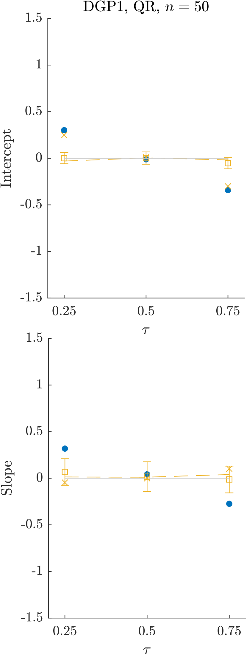
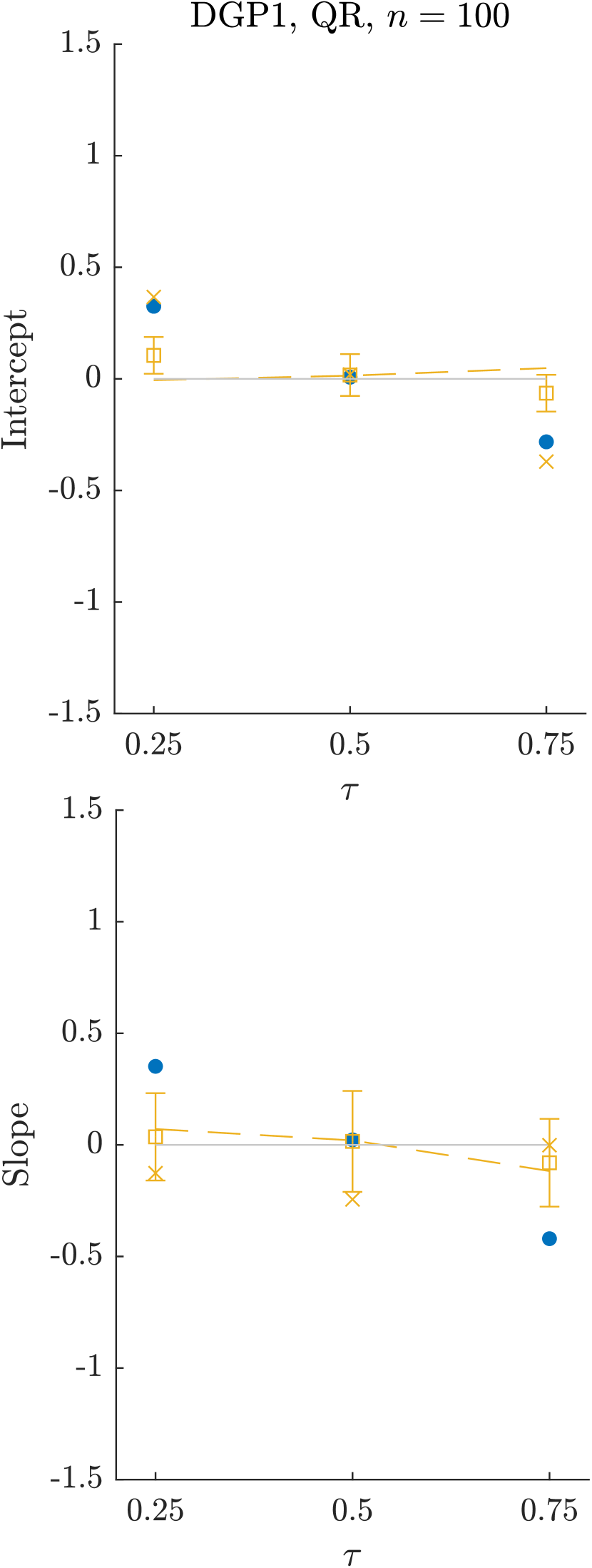
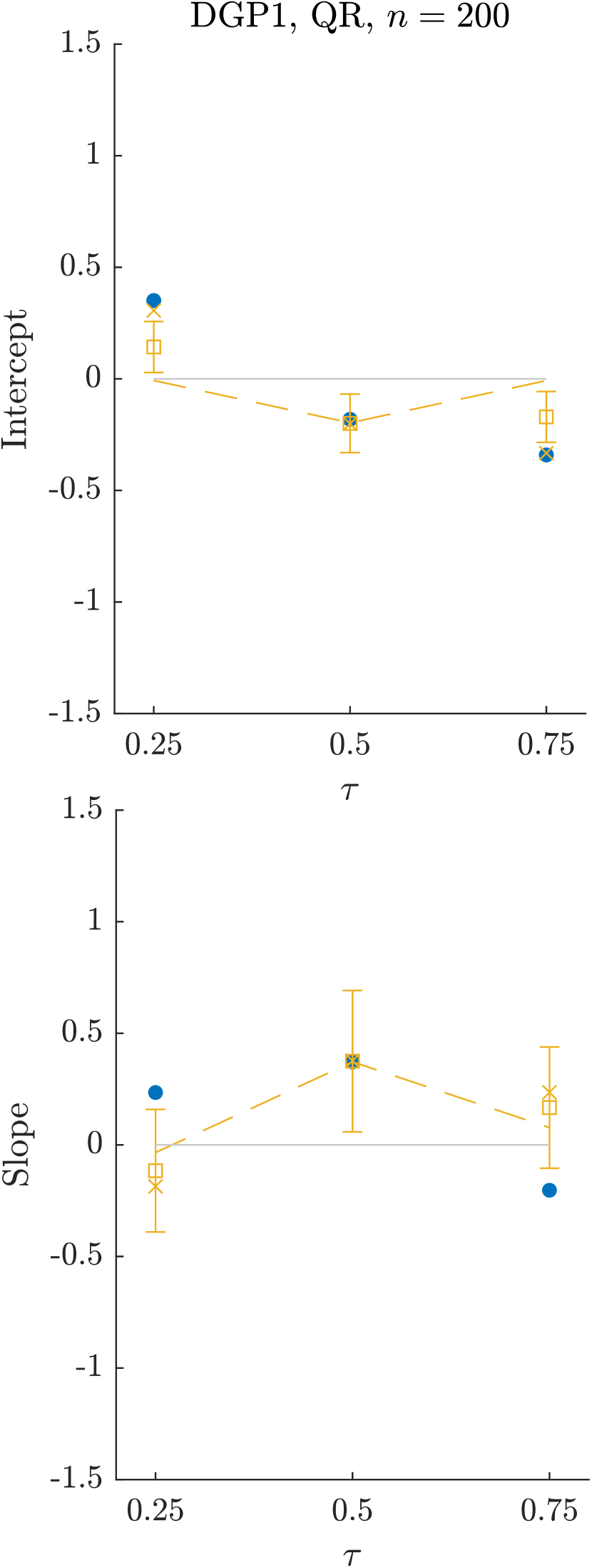
Notes: The panels display the bias (multiplied by $n$) of the intercept and the slope for classical QR without bias correction (blue dots), QR with the best feasible bias correction (gold squares), QR with the baseline feasible bias correction (gold crosses), and QR with infeasible bias correction (gold dashed line) for DGP1 with $n\in\{50,100,200\}$. The error bands (gold bars) correspond to $\Phi^{-1}(1-0.05/12)\times$ MCSE to account for the joint testing of 6 hypotheses. (Notice that the scaled MCSE of the estimator grows with $n$.) All results are based on 40,000 simulation repetitions.

Figure 3: Bias (multiplied by $n$) before and after correction for DGP2–DGP4

(a)

(b)

(c)

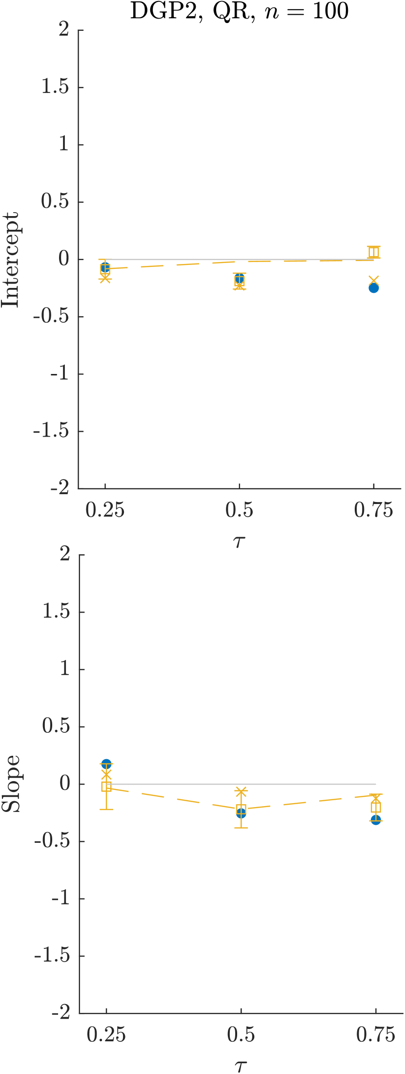
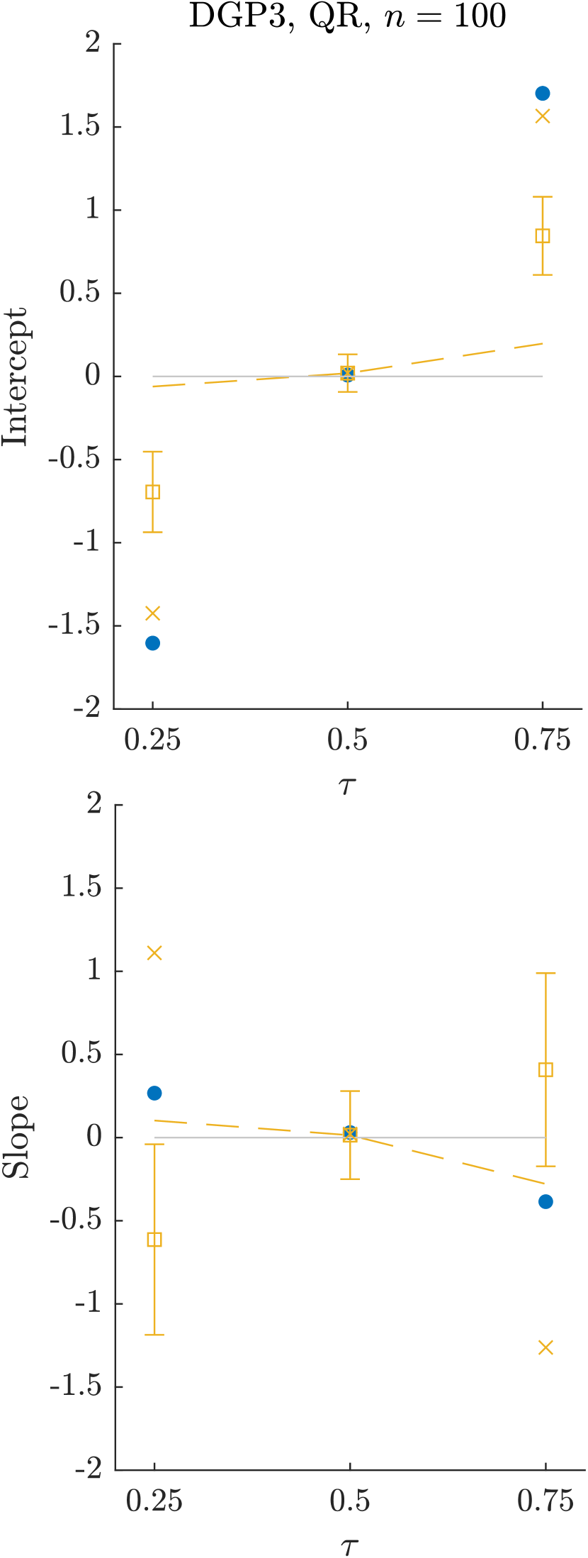
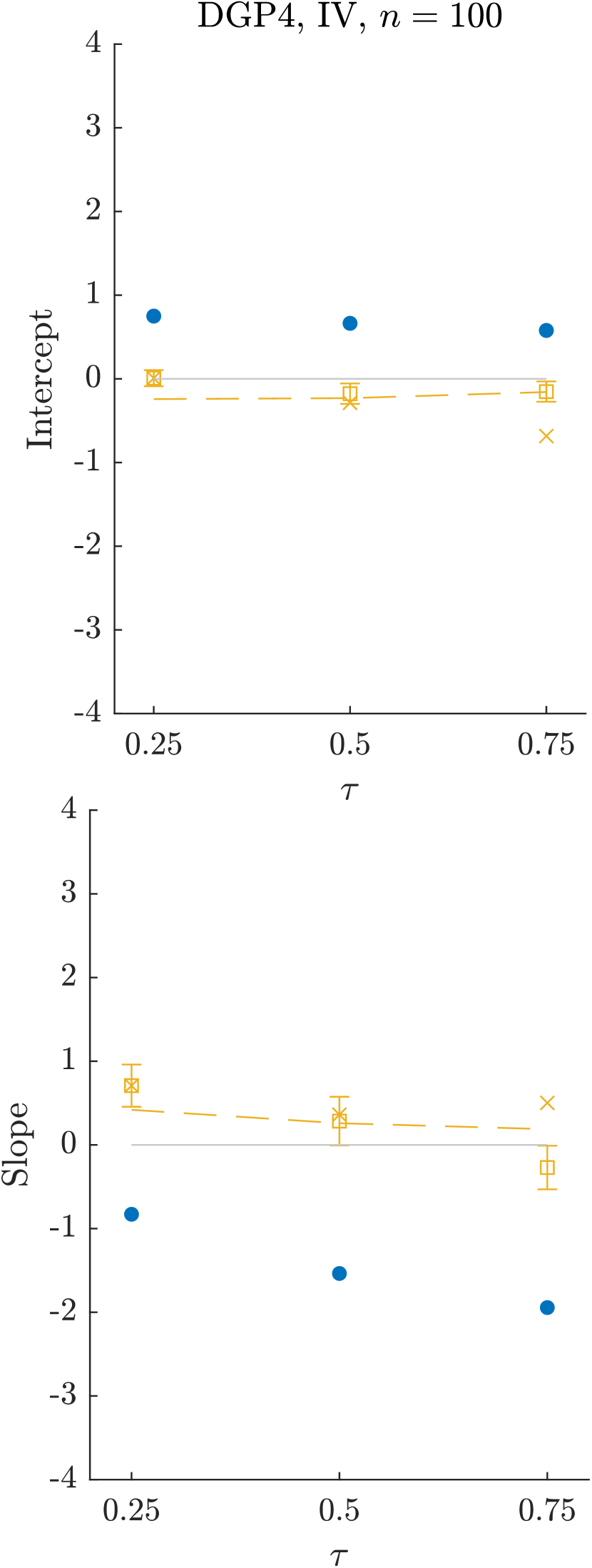
Notes: The panels display the bias (multiplied by $n$) of the intercept and the slope for classical QR without bias correction (blue dots), QR with the best feasible bias correction (gold squares), QR with the baseline feasible bias correction (gold crosses), and QR with infeasible bias correction (gold dashed line) for DGP2–DGP4 with $n=100$. We use classical QR for DGP2 and DGP3 and exact IVQR (implemented via the MILP formulation in Appendix D) for DGP4. The error bands (gold bars) correspond to $\Phi^{-1}(1-0.05/12)\times$ MCSE to account for the joint testing of 6 hypotheses. The DGP2 and DGP3 results are based on 40,000 simulation repetitions; the DGP4 results are based on 10,000 repetitions. For DGP4, the infeasible bias correction is based on the feasible formula applied to a simulated sample of 10,000,000 observations.

Figure 4: RMSE comparison of raw and bias-corrected estimators

(a)

(b)

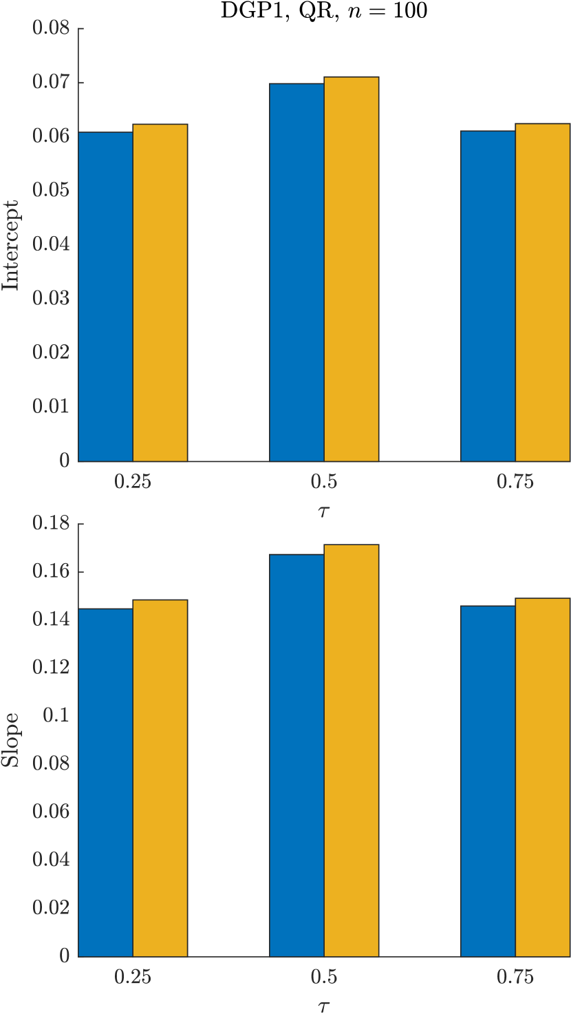
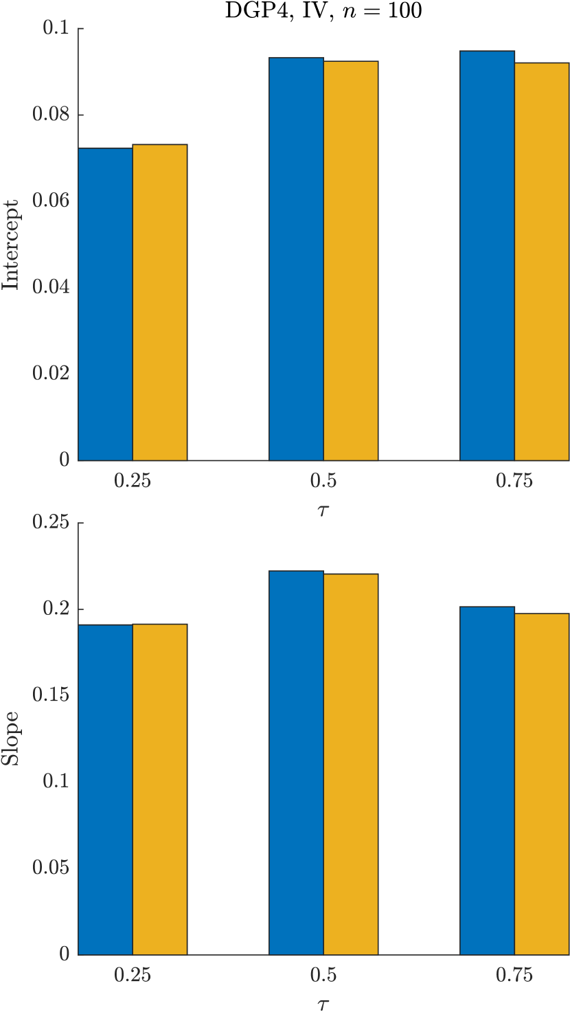
Notes: Panel (a) compares the RSME for classical QR without (blue) and with (gold) bias correction. Panel (b) compares the RMSE for exact IVQR (implemented via the MILP formulation in Appendix D) without (blue) and with (gold) bias correction. The results are based on 40,000 simulation repetitions.

5 Empirical application

The second-order bias matters most in applications with small sample sizes. We therefore illustrate our bias correction approach using the classical dataset of Engel (1857), analyzed by Koenker and Bassett (1982) and Koenker and Hallock (2001), among others. The data contain information on annual income and food expenditure (in Belgian francs) for $n=235$ Belgian working-class households and are obtained from the R package quantreg (Koenker, 2022). One feature of these data is the growing dispersion of the outcome variable (food expenditure) as a function of the regressor (income) (Koenker and Hallock, 2001), which is similar to our Monte Carlo designs. We divide the values of income and food expenditure by $1000$ so that the unit of measurement becomes a thousand Belgian francs. This makes the scale of the variables comparable to that in our Monte Carlo simulations, allowing us to use the same baseline bandwidth choices.

We estimate classical QRs of food expenditure ($Y$) on income ($W$) and a constant (blue dots). The bias-corrected estimators (gold squares) are obtained using the baseline bandwidth choice $h_{1,n}=A_{G}n^{-1/5}$, $h_{2,n}=A_{Q}n^{-1/7}$, and $h_{3,n}=A_{\kappa}n^{-2/15}$ with $(A_{G},A_{Q},A_{\kappa})=(1,1,1)$.

Figure 5 presents the results. Panel (a) shows the impact of bias correction. The results suggest that bias correction is more important at the upper tail, where we find differences between the classical QR and the bias-corrected estimates. After the bias correction, we observe more heterogeneity across quantile levels, suggesting that the second-order bias leads classical QR to underestimate this heterogeneity. Notice that there is a second-order bias even at the median (i.e., least absolute deviation) regression.

To investigate the sensitivity of our results to the choice of the three bandwidths, we also report the minimum and maximum bias-corrected estimates when $(A_{G},A_{Q},A_{\kappa})$ varies over the set $\mathcal{A}$ in equation (10). Our results suggest that bias-corrected estimates are insensitive to the bandwidth choice.

Panel (b) shows the individual contributions of the different components to the overall second-order bias. We can decompose the bias correction term as follows:

$$\hat{\theta}_{\tau}-\hat{\theta}_{bc}=\underbrace{\frac{1}{2}\hat{G}^{-1}\left[\hat{g}_{\tau}(\hat{\theta}_{\tau})-\hat{g}_{\tau}^{*}(-\hat{\theta}_{\tau})\right]}_{\text{(i)}}-\underbrace{\frac{1}{n}\hat{G}^{-1}\hat{\kappa}_{\tau}}_{\text{(ii)}}-\underbrace{\frac{1}{2n}G^{-1}\hat{Q}^{\prime}vec(\hat{\Omega})}_{\text{(iii)}}.$$

The main takeaway from the bias decomposition is that while all three components play a role, the sample moments term (i) can be very large and accounts for most of the bias at the upper tail quantiles. The QR estimates with the highest overall second-order bias have the largest contribution from the sample moments term ($\tau\in\{0.5,0.7\}$). These results suggest that one could reduce the worst-case bias substantially by only correcting the sample moment term, which is akin to a 1-step Newton correction (see Appendix E).

Figure 5: Quantile regression of annual food expenditure on income

(a) Impact of bias correction

(b) Composition of second-order bias

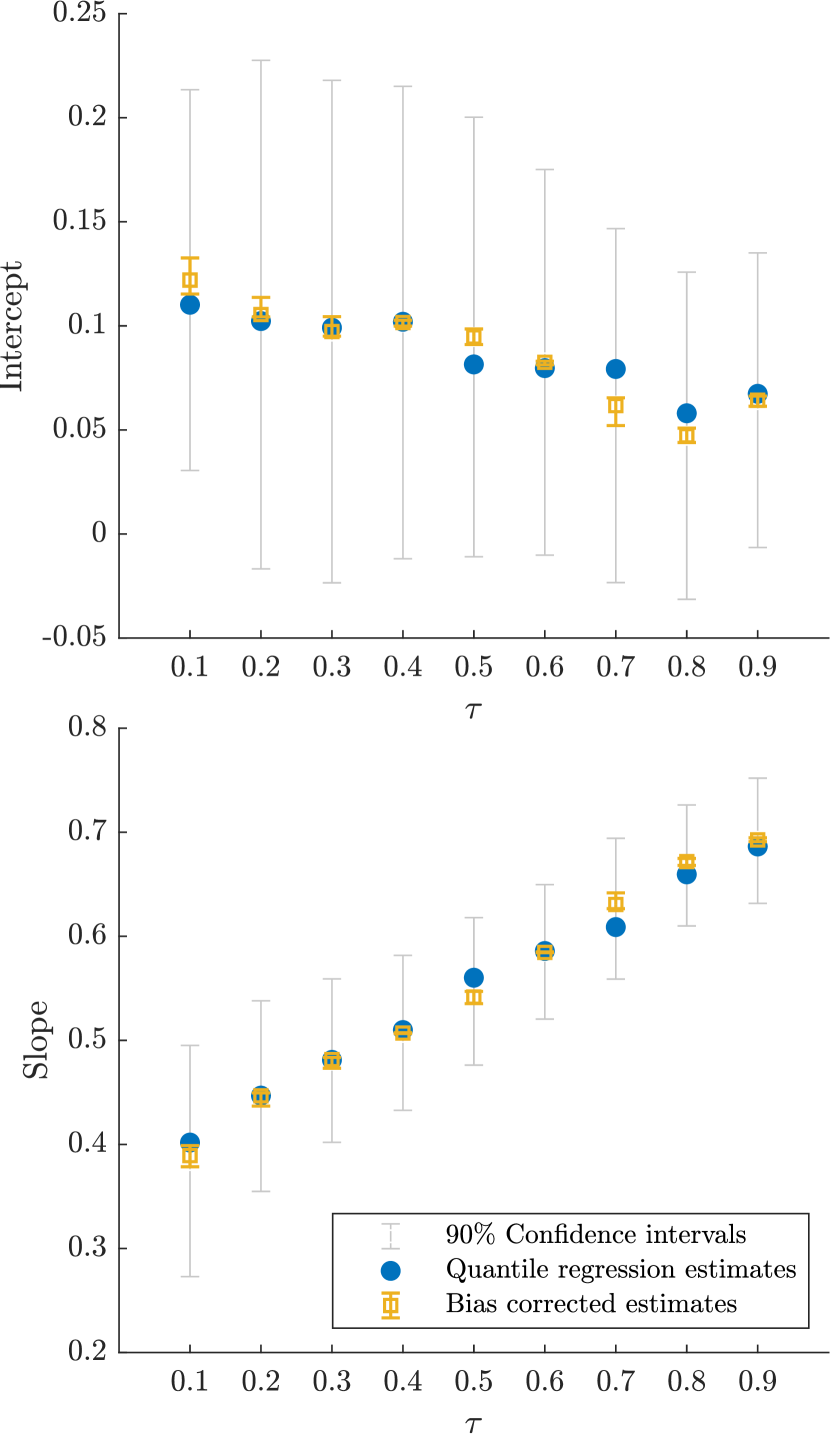
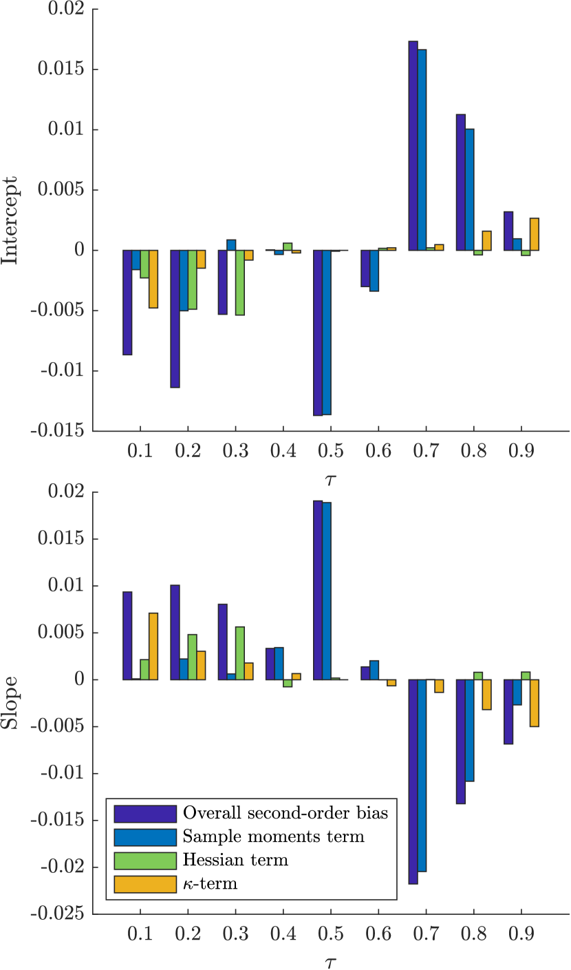
Notes: Panel (a) compares the classical QR estimates with (blue dots) and without (gold squares) bias correction, where $(A_{G},A_{Q},A_{\kappa})=(1,1,1)$. The bars indicate the minimum and the maximum of the estimates when varying $(A_{G},A_{Q},A_{\kappa})$ over the grid $\mathcal{A}$ defined in (10). Panel (b) shows the contributions of different bias components to the overall second-order bias.

6 Conclusion

We demonstrate that QR and IVQR estimators can exhibit a non-negligible second-order bias. We theoretically characterize this bias and use our results to derive a novel feasible bias correction method. Our method can effectively reduce the second-order bias at a very low computational cost and without substantially increasing RMSE.

Online appendix

Appendix A Bahadur-Kiefer representation, proofs

A.1 Auxiliary results for generic IVQR estimators

Lemma A.1.

Under Assumptions 2 and 3, $g_{\tau}(\theta)$ is three times continuously differentiable in $\theta$.

Proof.

By definition, $g_{\tau}(\theta)=\mathbb{E}(1\{Y\leq W^{\prime}\theta\}-\tau)Z=\mathbb{E}(\mathbb{E}(F_{Y}(W^{\prime}\theta|W,Z)-\tau)Z)$. The result then follows from the dominated convergence theorem. ∎

Lemma A.2.

Suppose Assumptions 2 and 3 hold. Then for any estimator $\hat{\theta}_{\tau}$ such that $\sup_{\tau\in[\varepsilon,1-\varepsilon]}\|\hat{\theta}_{\tau}-\theta_{\tau}\|=O_{p}\left({r^{-1}_{n}}\right)$ for some sequence $r_{n}\to\infty$, we have a representation

$$\hat{g}_{\tau}(\hat{\theta}_{\tau}) =\frac{1}{\sqrt{n}}B^{\circ}_{n}(\theta_{\tau})+\tau(\mathbb{E}Z-\mathbb{E}_{n}{Z})+\frac{1}{\sqrt{n}}B_{n}(\hat{\theta}_{\tau})$$

$$+G(\theta_{\tau})(\hat{\theta}_{\tau}-\theta_{\tau})+\frac{1}{2}(\hat{\theta}_{\tau}-\theta_{\tau})^{\prime}\partial_{\theta}G(\theta_{\tau})(\hat{\theta}_{\tau}-\theta_{\tau})+O_{p}\left(\frac{1}{r^{3}_{n}}\right),$$ (11)

where the remainder rate is uniform in $\tau\in[\varepsilon,1-\varepsilon]$.

Proof.

By definition,

$$\hat{g}_{\tau}(\hat{\theta}_{\tau}) =\mathbb{E}_{n}1\{Y\leq W^{\prime}\hat{\theta}_{\tau}\}Z-\tau\mathbb{E}_{n}Z$$

$$=\frac{1}{\sqrt{n}}B^{\circ}_{n}(\hat{\theta}_{\tau})+g^{\circ}(\hat{\theta}_{\tau})-\tau\mathbb{E}_{n}Z$$

$$=\frac{1}{\sqrt{n}}B^{\circ}_{n}(\theta_{\tau})+\frac{1}{\sqrt{n}}B_{n}(\hat{\theta}_{\tau})+\tau(\mathbb{E}Z-\mathbb{E}_{n}{Z})+g_{\tau}(\hat{\theta}_{\tau}).$$

By Lemma A.1, $g_{\tau}(\cdot)$ is three times continuously differentiable. Since $\theta$ is restricted to a compact set $\Theta$, the norm of the third derivative is bounded on $\Theta$. The Taylor theorem implies that there exist a neighborhood of $\theta_{\tau}$ such that for any $\theta$ in the neighborhood,

$$g_{\tau}(\theta)=G(\theta_{\tau})(\theta-\theta_{\tau})+\frac{1}{2}(\theta-\theta_{\tau})^{\prime}\partial_{\theta}G(\theta_{\tau})(\theta-\theta_{\tau})+R(\theta),$$

where $R(\theta)=O\left(\|\theta-\theta_{\tau}\|^{3}\right)$ uniformly in $\tau$. Then (11) follows immediately because $\hat{\theta}_{\tau}$ is a uniformly consistent estimator. ∎

Now let us study the large sample behavior of the term $B_{n}(\hat{\theta}_{\tau})$ in (11).

Lemma A.3.

Suppose that Assumptions 2 and 3 hold. For any pair of estimators $\hat{\theta}_{\tau}$ and $\hat{\theta}_{\tau}^{\ast}$ such that $\sup_{\tau\in[\varepsilon,1-\varepsilon]}\|\hat{\theta}_{\tau}^{\ast}-\hat{\theta}_{\tau}\|=O_{p}\left({r^{-1}_{n}}\right)$ for some sequence $r_{n}\to\infty$, we have

$$B_{n}(\hat{\theta}_{\tau})-B_{n}(\hat{\theta}_{\tau}^{\ast})=O_{p}\left(\sqrt{\frac{{\log r_{n}}}{r_{n}}}\right)+o_{p}\left(\frac{\log r_{n}}{n^{1/3}}\right)\quad\text{uniformly in }\tau\in[\varepsilon,1-\varepsilon].$$

Proof.

The proof relies on the arguments in Ota et al. (2019, Lemma 3) adapted to our setting. The idea is to verify the conditions of Lemma 1 of Ota et al. (2019), which follows from Corollary 5.1 in Chernozhukov et al. (2014) and use this corollary to prove the desired result.

Since $\sup_{\tau\in[\varepsilon,1-\varepsilon]}\|\hat{\theta}_{\tau}^{\ast}-\hat{\theta}_{\tau}\|=O_{p}\left({r^{-1}_{n}}\right)$, we have $P\left(\sup_{\tau\in[\varepsilon,1-\varepsilon]}\|\hat{\theta}_{\tau}^{\ast}-\hat{\theta}_{\tau}\|\leq{M_{n}}/{r_{n}}\right)\to 1$ for any sequence $M_{n}\to\infty$. Consider the functions

$$f_{\theta,h,\alpha}:\,(y,w,z)\mapsto\left(1\{y-w^{\prime}\theta\leq w^{\prime}h\}-1\{y-w^{\prime}\theta\leq 0\}\right)\alpha^{\prime}z$$

that constitute the function class

$$\mathcal{F}_{n} =\bigg{\{}f_{\theta,h,\alpha}:\,\,\theta\in\Theta,\|h\|\leq\frac{M_{n}}{r_{n}},\|\alpha\|=1\bigg{\}},$$

where $M_{n}$ is a sequence such that $M_{n}\to\infty$ and $M_{n}/r_{n}\to 0$. Let $\mathbb{G}_{n}$ be the standard empirical process operator on $\mathcal{F}_{n}$ with the data $(Y_{i},W_{i},Z_{i})$, $i=1,\dots,n$. By Assumption 3, $\mathcal{F}_{n}$ admits an envelope $F(y,w,z)\equiv\|z\|$.

Let us now verify the conditions in Lemma 1 of Ota et al. (2019). First, since

$$\left(1\left\{Y-W^{\prime}\theta\leq W^{\prime}h\right\}-1\left\{Y-W^{\prime}\theta\leq 0\right\}\right)^{2}=1\left\{\min(0,W^{\prime}h)<Y-W^{\prime}\theta\leq\max(0,W^{\prime}h)\right\},$$

we obtain

$$\mathbb{E}f_{\theta,h,\alpha}^{2}(Y,W,Z) =\mathbb{E}\left[\left(1\big{\{}Y-W^{\prime}\theta\leq W^{\prime}h\big{\}}-1\big{\{}Y-W^{\prime}\theta\leq 0\big{\}}\right)\alpha^{\prime}Z\right]^{2}$$

$$\leq\mathbb{E}\|Z\|^{2}\cdot\mathbb{E}1\bigg{\{}\min(0,W^{\prime}h)<Y-W^{\prime}\theta\leq\max(0,W^{\prime}h)\bigg{\}}$$

$$\leq km^{2/\gamma}\cdot\mathbb{E}1\bigg{\{}\min(0,W^{\prime}h)<Y-W^{\prime}\theta\leq\max(0,W^{\prime}h)\bigg{\}}$$

$$=km^{2/\gamma}\cdot\mathbb{E}\bigg{(}\mathbb{E}\left[\left|F_{Y}(W^{\prime}h+W^{\prime}\theta|W,Z)-F_{Y}(W^{\prime}\theta|W,Z)\right|\,\bigg{|}\,W,Z\right]\bigg{)}$$

$$\leq km^{2/\gamma}\cdot\mathbb{E}\bigg{(}\mathbb{E}\left[|W^{\prime}h|\sup_{y}f_{Y}(y|W,Z)\,\bigg{|}\,W,Z\right]\bigg{)}\leq k^{2}m^{4/\gamma}\bar{f}\|h\|=O\left(\frac{M_{n}}{r_{n}}\right),$$

where we used Assumptions 2 and the inequality

$$\mathbb{E}\|Z\|^{2}\leq k\max_{j=1,\dots,k}\mathbb{E}|Z_{j}|^{2}\leq k\max_{j=1,\dots,k}\left(\mathbb{E}|Z_{j}|^{\gamma}\right)^{2/\gamma}$$

in conjunction with Assumption 3.

Therefore, the variance parameter of the process is

$$\sigma_{n}^{2}\triangleq\sup_{f\in\mathcal{F}_{n}}\mathbb{E}f^{2}(Y,W,Z)=O\left(\frac{M_{n}}{r_{n}}\right).$$

Second, using Lemma 2 in Ota et al. (2019), we have

$$\mathbb{E}\max_{1\leq i\leq n}F^{2}(Y_{i},W_{i},Z_{i})=\mathbb{E}\max_{1\leq i\leq n}\|Z_{i}\|^{2}=o(n^{2/\gamma}).$$

Third, because the function class $\mathcal{F}_{n}$ is a VC class (Vapnik and Chervonenkis, 1971) with the envelope $\|Z\|$, there exist constants $A$ and $V$ independent of $n$ such that the standard entropy bound

$$\sup_{Q}N\left(\mathcal{F}_{n},\|\cdot\|_{Q,2},\eta\|Z\|_{Q,2}\right)\leq(A/\eta)^{V},\text{ for all }\eta\in(0,1]$$

holds (e.g., van der Vaart and Wellner, 1996, Section 2.6). Here the supremum is taken over all finitely discrete measures $Q$ and $\|\cdot\|_{Q,2}$ is the $L^{2}(Q)$ norm.

Finally, applying Lemma 1 in Ota et al. (2019), we obtain

$$\mathbb{E}\sup_{\theta\in\Theta,\|h\|\leq\frac{M_{n}}{r_{n}},\|\alpha\|=1}\|\mathbb{G}_{n}f_{\theta,h,\alpha}\|\lesssim\sqrt{V\sigma_{n}^{2}\log(Am/\sigma_{n})}+\frac{V\sqrt{\mathbb{E}\max_{1\leq i\leq n}\|Z_{i}\|^{2}}}{\sqrt{n}}\log(Am/\sigma_{n})$$

$$=O\left(\sqrt{\frac{\log r_{n}}{r_{n}}}\right)+o\left(\frac{\log r_{n}}{n^{\frac{\gamma-2}{2\gamma}}}\right),$$ (12)

where the last equality holds by choosing $M_{n}\to\infty$ sufficiently slowly. Note that the right-hand side of this equation does not depend on $\tau$. Consequently, by the definition of the norm and equation (12),

$$\sup_{\tau\in[\varepsilon,1-\varepsilon]}\|B_{n}(\hat{\theta}_{\tau})-B_{n}(\hat{\theta}_{\tau}^{*})\| =\sup_{\tau\in[\varepsilon,1-\varepsilon]}\max_{\|\alpha\|=1}\bigg{|}\mathbb{G}_{n}f_{\hat{\theta}_{\tau},(\hat{\theta}_{\tau}-\hat{\theta}_{\tau}^{*}),\alpha}\bigg{|}$$

$$=O_{p}\left(\sqrt{\frac{{\log r_{n}}}{r_{n}}}\right)+o_{p}\left(\frac{\log r_{n}}{n^{\frac{\gamma-2}{2\gamma}}}\right),$$

where the last equality holds by Markov’s inequality.

∎

A.2 Auxiliary results for exact estimators

Lemma A.4.

Under Assumptions 1.1, 2 and 3, $\sup_{\tau\in[\varepsilon,1-\varepsilon]}\|\hat{\theta}_{\tau}-\theta_{\tau}\|=o_{p}\left(1\right)$, where $\hat{\theta}_{\tau}=\hat{\theta}_{\tau,p}$ for any $p\in[1,\infty]$ or $\hat{\theta}_{\tau}=\hat{\theta}_{\tau,\text{QR}}$.

Proof.

We give the proof for $\hat{\theta}_{\tau}=\hat{\theta}_{\tau,p}$. Uniform consistency for the case of $\hat{\theta}_{\tau}=\hat{\theta}_{\tau,\text{QR}}$ was established by Angrist et al. (2006, Theorem 3).

By Assumption 1.1,

$$\arg\min_{\theta\in\Theta}\|g_{\tau}(\theta)\|_{p}=\theta_{\tau}.$$

Assumptions 2 and 3 imply that the function class

$$\left\{(w,y,z)\mapsto z(1\{y\leq w^{\prime}\theta\}-\tau),\leavevmode\nobreak\ \tau\in[\varepsilon,1-\varepsilon],\leavevmode\nobreak\ \theta\in\Theta\right\}$$

is Donsker (compare with the function class $\mathcal{F}_{n}$ in the proof of Lemma A.3) and thus Glivenko-Cantelli, and hence

$$\sup_{\theta\in\Theta,\tau\in[\varepsilon,1-\varepsilon]}|\hat{g}_{\tau}(\theta)-g_{\tau}(\theta)|=\sup_{\theta\in\Theta,\tau\in[\varepsilon,1-\varepsilon]}|(\mathbb{E}_{n}-\mathbb{E})Z_{i}(1\{Y_{i}\leq W^{\prime}\theta\}-\tau)|\stackrel{{\scriptstyle a.s.}}{{\rightarrow}}0.$$

By the argmin theorem (e.g., Theorem 2.1 in Newey and McFadden, 1994) applied to $Q_{n}(\theta,\tau)\triangleq\|\hat{g}_{\tau}(\theta)\|_{p}$, we get $\sup_{\tau\in[\varepsilon,1-\varepsilon]}\|\hat{\theta}_{\tau,p}-\theta_{\tau}\|=o_{p}\left(1\right)$. ∎

Lemma A.5.

Under Assumptions 1–3, for any exact QR estimator $\hat{\theta}_{\tau,\text{QR}}$ as defined in equation (2), we have

$$\sup_{\tau\in[\varepsilon,1-\varepsilon]}\|\hat{\theta}_{\tau,\text{QR}}-\theta_{\tau}\| =O_{p}\left(\frac{1}{\sqrt{n}}\right),$$ (13)

$$\sup_{\tau\in[\varepsilon,1-\varepsilon]}\|\hat{g}_{\tau}(\hat{\theta}_{\tau,\text{QR}})\|_{p} =O_{p}\left(\frac{k}{n}\right).$$

Proof.

Equation (13) follows from Theorem 3 in Angrist et al. (2006).

The exact QR estimators yield exact zeros of the subgradient

$$\frac{1}{n}\sum_{i=1}^{n}(\tau-h(Y_{i}-W_{i}^{\prime}\theta))W_{i},$$

where the multi-valued function $h(u)$ is defined as $1\{u<0\}$ for $u\neq 0$ and $h(0)\triangleq[0,1]$ for $u=0$. The subgradient function differs from sample moment functions by the fraction of observations with $Y_{i}=W_{i}^{\prime}\hat{\theta}_{\tau,\text{QR}}$. Note that under Assumption 2, $Y_{i}$ has density with respect to the Lebesgue measure conditional on $W_{i}$. Thus the observations $(Y_{i},W_{i})$ are in general position with probability 1 (see Definition 2.1 and the subsequent discussion in Koenker, 2005). Because the observations are in general position with probability 1, there are at most $k$ terms like that, and so $\sup_{\tau\in[\varepsilon,1-\varepsilon]}\|\hat{g}_{\tau}(\hat{\theta}_{\tau,\text{QR}})\|_{p}=O_{p}\left({k}/{n}\right)$. ∎

Lemma A.6.

Under Assumptions 1, 2, and 3, for any estimator $\hat{\theta}_{\tau}=\hat{\theta}_{\tau,p}$ that minimizes $\|\hat{g}_{\tau}(\theta)\|_{p}$, we have

$$\sup_{\tau\in[\varepsilon,1-\varepsilon]}\|\hat{\theta}_{\tau}-\theta_{\tau}\| =O_{p}\left(\frac{1}{\sqrt{n}}\right),$$ (14)

$$\sup_{\tau\in[\varepsilon,1-\varepsilon]}\|\hat{\theta}_{\tau}-\hat{\xi}_{\tau}\| =o_{p}\left(\frac{1}{\sqrt{n}}\right),$$ (15)

$$\sup_{\tau\in[\varepsilon,1-\varepsilon]}\|\hat{g}_{\tau}(\hat{\theta}_{\tau})\|_{p} =o_{p}\left(\frac{1}{\sqrt{n}}\right),$$ (16)

where $\hat{\xi}_{\tau}$ is defined in equation (4).

Proof.

The proof proceeds in four steps.

Step 1. Under the assumptions of the lemma, the empirical process $B_{n}^{\circ}(\theta)$ is Donsker (see proof of Lemma A.3 above) and thus asymptotically stochastically equicontinuous (see discussion in van der Vaart and Wellner, 1996, Section 2.1.2; also Theorem 1.5.7 and Problem 2.1.5 in the same book).

Step 2. By definition, $\sqrt{n}(\hat{\xi}_{\tau}-\theta_{\tau})$ can be written as

$$\sqrt{n}(\hat{\xi}_{\tau}-\theta_{\tau}) =-G^{-1}_{\tau}\sqrt{n}\left[\tau(\mathbb{E}Z-\mathbb{E}_{n}Z)+\frac{1}{\sqrt{n}}B^{\circ}_{n}(\theta_{\tau})\right],$$ (17)

where $\theta_{\tau}$ and $G_{\tau}\triangleq\partial_{\theta}g_{\tau}(\theta_{\tau})$ are well-defined by Assumption 1 . This class of functions indexed by $\tau$ is Donsker by similar arguments as in Lemma A.3 (note that the parameter $\tau$ enters this class only through $\theta_{\tau}$ and through the linear term $\tau Z_{i}$). The Donsker property implies

$$\sup_{\tau\in[\varepsilon,1-\varepsilon]}\|\hat{\xi}_{\tau}-\theta_{\tau}\|=O_{p}\left(\frac{1}{\sqrt{n}}\right).$$ (18)

By Lemma A.2 applied to $\hat{\xi}_{\tau}$,

$$\hat{g}_{\tau}(\hat{\xi}_{\tau}) =\frac{1}{\sqrt{n}}B^{\circ}_{n}(\theta_{\tau})+\tau(\mathbb{E}Z-\mathbb{E}_{n}{Z})+\frac{1}{\sqrt{n}}B_{n}(\hat{\xi}_{\tau})$$

$$+g(\theta_{\tau})+G(\theta_{\tau})(\hat{\xi}_{\tau}-\theta_{\tau})+\frac{1}{2}(\hat{\xi}_{\tau}-\theta_{\tau})^{\prime}\partial_{\theta}G(\theta_{\tau})(\hat{\xi}_{\tau}-\theta_{\tau})+O_{p}\left(n^{-\frac{3}{2}}\right).$$

Then after substituting the first equation in (18) into the term $G(\theta_{\tau})(\hat{\xi}_{\tau}-\theta_{\tau})$, we have

$$\hat{g}_{\tau}(\hat{\xi}_{\tau})=\frac{1}{\sqrt{n}}B_{n}(\hat{\xi}_{\tau})+O_{p}\left(\frac{1}{n}\right).$$

So by Step 1, $\hat{g}_{\tau}(\hat{\xi}_{\tau})=O_{p}\left(n^{-\frac{1}{2}}\right)$.

Since $\hat{\theta}_{\tau,p}$ is defined as the estimator attaining the minimal $p$-norm,

$$\sup_{\tau\in[\varepsilon,1-\varepsilon]}\|\hat{g}_{\tau}(\hat{\theta}_{\tau,p})\|_{p}\leq\sup_{\tau\in[\varepsilon,1-\varepsilon]}\|\hat{g}_{\tau}(\hat{\xi}_{\tau})\|_{p}=O_{p}\left(n^{-\frac{1}{2}}\right).$$

Step 3. Consider $\hat{\xi}^{(2)}_{\tau}\triangleq\hat{\xi}_{\tau}-G^{-1}{B_{n}(\hat{\xi}_{\tau})}/{\sqrt{n}}$. By equation (18), $\hat{\xi}_{\tau}$ is uniformly consistent, and hence $\hat{\xi}^{(2)}_{\tau}=\hat{\xi}_{\tau}+o_{p}\left({1}/{\sqrt{n}}\right)$ uniformly in $\tau\in[\varepsilon,1-\varepsilon]$ since $B_{n}$ is stochastically equicontinuous (Step 1). Then by the stochastic equicontinuity of $B^{\circ}_{n}$ (Step 1) and Lemma A.2 applied to $\hat{\xi}^{(2)}_{\tau}$, uniformly in $\tau\in[\varepsilon,1-\varepsilon]$,

$$\hat{g}_{\tau}(\hat{\xi}^{(2)}_{\tau})=\frac{B_{n}^{\circ}(\hat{\xi}^{(2)}_{\tau})-B^{\circ}_{n}(\hat{\xi}_{\tau})}{\sqrt{n}}+o_{p}\left(\frac{1}{\sqrt{n}}\right)=o_{p}\left(\frac{1}{\sqrt{n}}\right).$$

This implies

$$\sup_{\tau\in[\varepsilon,1-\varepsilon]}\|\hat{g}_{\tau}(\hat{\theta}_{\tau,p})\|_{p}\leq\sup_{\tau\in[\varepsilon,1-\varepsilon]}\|\hat{g}_{\tau}(\hat{\xi}^{(2)}_{\tau})\|_{p}=o_{p}\left(n^{-\frac{1}{2}}\right).$$

which establishes (16).

Step 4. By Lemma A.4, $\sup_{\tau\in[\varepsilon,1-\varepsilon]}\|\hat{\theta}_{\tau,p}-\theta_{\tau}\|=O_{p}\left({r^{-1}_{n}}\right)$ for some $r_{n}\to\infty$. By Lemma A.2 and Steps 1 and 2, $\hat{\theta}_{\tau,p}$ satisfies

$$G(\theta_{\tau})(\hat{\theta}_{\tau,p}-\theta_{\tau})+\frac{1}{2}(\hat{\theta}_{\tau,p}-\theta_{\tau})^{\prime}\partial_{\theta}G(\theta_{\tau})(\hat{\theta}_{\tau,p}-\theta_{\tau})$$

$$=\hat{g}_{\tau}(\hat{\theta}_{\tau,p})-\frac{1}{\sqrt{n}}B^{\circ}_{n}(\theta_{\tau})-\tau(\mathbb{E}Z-\mathbb{E}_{n}{Z})-\frac{1}{\sqrt{n}}B_{n}(\hat{\theta}_{\tau,p})+O_{p}\left(\frac{1}{r_{n}^{3}}\right)$$

$$=O_{p}\left(\frac{1}{\sqrt{n}}\right)+O_{p}\left(\frac{1}{r_{n}^{3}}\right),$$ (19)

uniformly in $\tau\in[\varepsilon,1-\varepsilon]$.

By Assumption 1.2, we can multiply the last equation by $G^{-1}(\theta_{\tau})$ and obtain

$$\hat{\theta}_{\tau,p}-\theta_{\tau}+O_{p}\left(\frac{1}{r_{n}^{2}}\right) =O_{p}\left(\frac{1}{\sqrt{n}}\right)+O_{p}\left(\frac{1}{r_{n}^{3}}\right),$$

which implies we can take $r_{n}=\sqrt{n}$ by a fixed point argument, which is discussed in detail in Step 3 of the proof of Lemma A.7 below. This implies (14).

By uniform consistency of $\hat{\theta}_{\tau,p}$ and Step 1,

$$\sup_{\tau\in[\varepsilon,1-\varepsilon]}\|B_{n}(\hat{\theta}_{\tau,p})\|=\sup_{\tau\in[\varepsilon,1-\varepsilon]}\|B_{n}^{\circ}(\hat{\theta}_{\tau,p})-B_{n}^{\circ}(\theta_{\tau})\|=o_{p}(1).$$

Lemma A.2 applied to $\hat{\theta}_{\tau,p}$ yields

$$\hat{\theta}_{\tau,p} =\hat{\xi}_{\tau}-G^{-1}(\theta_{\tau})\frac{1}{2}(\hat{\theta}_{\tau,p}-\theta_{\tau})^{\prime}\partial_{\theta}G(\theta_{\tau})(\hat{\theta}_{\tau,p}-\theta_{\tau})+G^{-1}(\theta_{\tau})\hat{g}_{\tau}(\hat{\theta}_{\tau,p})$$

$$-\frac{1}{\sqrt{n}}G^{-1}(\theta_{\tau})B_{n}(\hat{\theta}_{\tau,p})+O_{p}\left(n^{-3/2}\right).$$

The term $G^{-1}(\theta_{\tau})2^{-1}(\hat{\theta}_{\tau,p}-\theta_{\tau})^{\prime}\partial_{\theta}G(\theta_{\tau})(\hat{\theta}_{\tau,p}-\theta_{\tau})$ is $O_{p}(n^{-1})$. The term $G^{-1}(\theta_{\tau})\hat{g}_{\tau}(\hat{\theta}_{\tau,p})$ is $o_{p}(n^{-1/2})$ by Step 3. The term $n^{-1/2}G^{-1}(\theta_{\tau})B_{n}(\hat{\theta}_{\tau,p})$ is $o_{p}(n^{-1/2})$ by stochastic equicontinuity of $B_{n}$ (Step 1) and uniform consistency of $\hat{\theta}_{\tau,p}$. Therefore,

$$\hat{\theta}_{\tau,p} =\hat{\xi}_{\tau}+o_{p}\left(n^{-\frac{1}{2}}\right)$$

uniformly in $\tau\in[\varepsilon,1-\varepsilon]$. This proves (15). ∎

The results of the previous lemma can be further refined.

Lemma A.7.

Under Assumptions 1–3, for any estimator $\hat{\theta}_{\tau,p}$ that minimizes $\|\hat{g}_{\tau}(\theta)\|_{p}$, we have

$$\sup_{\tau\in[\varepsilon,1-\varepsilon]}\|\hat{g}_{\tau}(\hat{\theta}_{\tau,p})\|_{p} =O_{p}\left(\frac{\log n}{n^{1-\frac{2}{\gamma}}}\right).$$

Proof.

The proof proceeds in four steps.

Step 1. By Lemma A.3 and A.6 applied to $\hat{\theta}_{\tau,p}$ and $\theta_{\tau}$,

$$B_{n}(\hat{\theta}_{\tau,p})=B_{n}(\hat{\theta}_{\tau,p})-B_{n}(\theta_{\tau})=O_{p}\left(\sqrt{\frac{{\log\sqrt{n}}}{\sqrt{n}}}\right)+o_{p}\left(\frac{\log n}{n^{\frac{\gamma-2}{2\gamma}}}\right)\quad\text{uniformly in }\tau\in[\varepsilon,1-\varepsilon].$$

Since $\frac{\gamma-2}{2\gamma}\geq\frac{1}{3}$ for $\gamma\geq 6$,

$$B_{n}(\hat{\theta}_{\tau,p})=O_{p}\left(\frac{\sqrt{\log n}}{n^{1/4}}\right)\quad\text{uniformly in }\tau\in[\varepsilon,1-\varepsilon].$$

Step 2. Consider the estimator

$$\hat{\xi}_{\tau}^{(2)} \triangleq\hat{\xi}_{\tau}-\frac{G^{-1}(\theta_{\tau})B_{n}(\hat{\theta}_{\tau,p})}{\sqrt{n}},$$

where, by Step 1, ${G^{-1}(\theta_{\tau})B_{n}(\hat{\theta}_{\tau,p})}/{\sqrt{n}}=O_{p}\left({n^{-3/4}\sqrt{\log n}}\right)$.

By Lemma A.2, we get

$$\hat{g}_{\tau}(\hat{\xi}_{\tau}^{(2)}) =\frac{1}{\sqrt{n}}B^{\circ}_{n}(\theta_{\tau})+(\tau\mathbb{E}Z-\tau\mathbb{E}_{n}Z)+\frac{1}{\sqrt{n}}B_{n}(\hat{\xi}_{\tau}^{(2)})$$

$$+G(\theta_{\tau})(\hat{\xi}_{\tau}^{(2)}-\theta_{\tau})+(\hat{\xi}_{\tau}^{(2)}-\theta_{\tau})^{\prime}\frac{\partial G(\theta_{\tau})}{\partial\theta}(\hat{\xi}_{\tau}^{(2)}-\theta_{\tau})+O_{p}\left(\frac{1}{n^{3/2}}\right).$$ (20)

Then, by definition of $\hat{\xi}_{\tau}^{(2)}$,

$$\hat{g}_{\tau}(\hat{\xi}_{\tau}^{(2)})= \frac{B_{n}(\hat{\xi}_{\tau}^{(2)})-B_{n}(\hat{\theta}_{\tau,p})}{\sqrt{n}}+(\hat{\xi}_{\tau}^{(2)}-\theta_{\tau})^{\prime}\frac{\partial G(\theta_{\tau})}{\partial\theta}(\hat{\xi}_{\tau}^{(2)}-\theta_{\tau})+O_{p}\left(\frac{1}{n^{3/2}}\right).$$ (21)

Define $r_{n}$ to be a sequence satisfying $\sup_{\tau\in[\varepsilon,1-\varepsilon]}\|\hat{\theta}_{\tau,p}-\hat{\xi}_{\tau}^{(2)}\|=O_{p}(r_{n}^{-1})$ (Lemma A.6 implies uniform consistency of $\hat{\theta}_{\tau,p}$ and that $r_{n}$ can be taken to be at least $\sqrt{n}$).

By Lemma A.3,

$$B_{n}(\hat{\xi}_{\tau}^{(2)})-B_{n}(\hat{\theta}_{\tau,p})=O_{p}\left(\sqrt{\frac{{\log r_{n}}}{r_{n}}}\right)+o_{p}\left(\frac{\log r_{n}}{n^{\frac{\gamma-2}{2\gamma}}}\right),$$

Then (21) becomes

$$\hat{g}_{\tau}(\hat{\xi}_{\tau}^{(2)})=O_{p}\left(\frac{\sqrt{\log n}}{\sqrt{nr_{n}}}\right)+o_{p}\left(\frac{\log n}{{n^{1-\frac{1}{\gamma}}}}\right),$$ (22)

where we replaced $\log r_{n}$ with the faster growing sequence $\log\sqrt{n}=O(\log n)$.

By Lemma A.2 applied to $\hat{\theta}_{\tau,p}$ and the definition of $\hat{\xi}_{\tau}$,

$$\hat{\theta}_{\tau,p} =\hat{\xi}_{\tau}+G^{-1}(\theta_{\tau})\hat{g}_{\tau}(\hat{\theta}_{\tau,p})-\frac{G^{-1}(\theta_{\tau})B_{n}(\hat{\theta}_{\tau,p})}{\sqrt{n}}$$

$$-G^{-1}(\theta_{\tau})(\hat{\theta}_{\tau,p}-\theta_{\tau})^{\prime}\frac{\partial G(\theta_{\tau})}{\partial\theta}(\hat{\theta}_{\tau,p}-\theta_{\tau})+O_{p}\left(\frac{1}{n^{3/2}}\right).$$

So by (20) and the definition of $\hat{\xi}_{\tau}^{(2)}$, we get

$$\hat{\theta}_{\tau,p}-\hat{\xi}_{\tau}^{(2)}=G^{-1}(\theta_{\tau})\hat{g}_{\tau}(\hat{\theta}_{\tau,p})+O_{p}(n^{-1}),$$

which implies we can take $r_{n}^{-1}$ as the rate of $\hat{g}_{\tau}(\hat{\theta}_{\tau,p})=O_{p}(r_{n}^{-1})$.

Step 3. By definition of $\hat{\theta}_{\tau,p}$, $\sup_{\tau\in[\varepsilon,1-\varepsilon]}\|\hat{g}_{\tau}({\hat{\theta}_{\tau,p}})\|_{p}\leq\sup_{\tau\in[\varepsilon,1-\varepsilon]}\|\hat{g}_{\tau}({\hat{\xi}_{\tau}^{(2)}})\|_{p}$. Then from (22), we obtain

$$\sup_{\tau\in[\varepsilon,1-\varepsilon]}\|\hat{g}_{\tau}({\hat{\theta}_{\tau,p}})\|_{p}\leq\sup_{\tau\in[\varepsilon,1-\varepsilon]}\|\hat{g}_{\tau}({\hat{\xi}_{\tau}^{(2)}})\|_{p}=O_{p}\left(\frac{\sqrt{\log n}}{\sqrt{nr_{n}}}\right)+o_{p}\left(\frac{\log n}{{n^{1-\frac{1}{\gamma}}}}\right).$$

On the right-hand side of this inequality, suppose that the first term dominates the second term. Then we have

$$(r_{n}^{-1})^{\frac{1}{2}} =O\left(\frac{\sqrt{\log n}}{n^{\frac{1}{2}-\frac{1}{\gamma}}}\right),$$

or, equivalently,

$$r_{n}^{-1} =O\left(\frac{\log n}{n^{1-\frac{2}{\gamma}}}\right).$$

By Step 2, it implies the statement of the lemma.

Suppose, instead, that the second term dominates the first term. Then by Step 2, $r_{n}^{-1}=O\left(n^{-1+\frac{1}{\gamma}}\log n\right)$. The statement of the lemma follows.

∎

A.3 Proof of Theorem 1

The proof of Theorem 1 summarizes the results of auxiliary lemmas in Appendices A.1 and A.2.

Step 1 (Uniform consistency). The estimators under consideration are uniformly consistent, $\sup_{\tau\in[\varepsilon,1-\varepsilon]}\|\hat{\theta}_{\tau}-\theta_{\tau}\|=O_{p}\left({1}/{\sqrt{n}}\right)$. Specifically, the QR estimator is analyzed in Lemma A.5; the exact IVQR estimator is analyzed in Lemma A.6.

Step 2 (Generic stochastic expansion). By Step 1, we can apply Lemma A.2 with $r_{n}=\sqrt{n}$ to obtain

$$\hat{\theta}_{\tau}-G^{-1}\hat{g}_{\tau}(\hat{\theta}_{\tau})=\hat{\xi}_{\tau}-G^{-1}\left[\frac{B_{n}(\hat{\theta}_{\tau})}{\sqrt{n}}+\frac{1}{2}(\hat{\theta}_{\tau}-\theta_{\tau})^{\prime}\partial_{\theta}G(\theta_{\tau})(\hat{\theta}_{\tau}-\theta_{\tau})\right]+O_{p}\left(\frac{1}{n^{3/2}}\right).$$

Step 3 (Bounds on remainder in asymptotic linear expansion). Now we can use the remaining lemmas to bound the orders of the terms in the expansion. The result in equation (6) follows from Lemma A.3 with $\hat{\theta}_{\tau}^{\ast}=\theta_{\tau}$ and $r_{n}=\sqrt{n}$. The first equation in (5) is stated in Lemma A.5. Similarly, Lemma A.7 yields the second equation in (5). As a result, we have

$$\sup_{\tau\in[\varepsilon,1-\varepsilon]}\|\hat{\theta}_{\tau}-\hat{\xi}_{\tau}\|=O_{p}\left(\frac{\sqrt{\log n}}{n^{3/4}}\right),$$ (23)

which is a uniform Bahadur-Kiefer expansion for both QR and exact IVQR estimators.

Step 4 (Analysis of quadratic term). The empirical process $\sqrt{n}(\hat{\xi}_{\tau}-\theta_{\tau})$ indexed by $\tau\in[\varepsilon,1-\varepsilon]$ is Donsker (see Step 2 of Lemma A.6), which implies (7), i.e.,

$$\sup_{\tau\in[\varepsilon,1-\varepsilon]}\|\hat{\xi}_{\tau}-\theta_{\tau}\|=O_{p}\left(\frac{1}{n^{1/2}}\right).$$ (24)

Then by Step 3, we have, uniformly in $\tau\in[\varepsilon,1-\varepsilon]$,

$$(\hat{\theta}_{\tau}-\theta_{\tau})^{\prime}\partial_{\theta}G(\theta_{\tau})(\hat{\theta}_{\tau}-\theta_{\tau})=(\hat{\xi}_{\tau}-\theta_{\tau})^{\prime}\partial_{\theta}G(\theta_{\tau})(\hat{\xi}_{\tau}-\theta_{\tau})+O_{p}\left(\frac{\sqrt{\log n}}{n^{5/4}}\right).$$

Hence, the expansion in Step 2 becomes

$$\hat{\theta}_{\tau}=\hat{\xi}_{\tau}+G^{-1}\left[\hat{g}_{\tau}(\hat{\theta}_{\tau})-\frac{B_{n}(\hat{\theta}_{\tau})}{\sqrt{n}}-\frac{1}{2}(\hat{\xi}_{\tau}-\theta_{\tau})^{\prime}\partial_{\theta}G(\theta_{\tau})(\hat{\xi}_{\tau}-\theta_{\tau})\right]+R_{n,\tau},$$

with $\sup_{\tau\in[\varepsilon,1-\varepsilon]}\|R_{n,\tau}\|=O_{p}\left(\frac{\sqrt{\log n}}{n^{5/4}}\right)$.

∎

Appendix B Second-order bias correction, proofs

B.1 Auxiliary results

Lemma B.1.

Consider any random sequence $\hat{\theta}\in\Theta$ a.s. Under Assumption 3, the following expectations exist,

$$\mathbb{E}\|\hat{g}_{\tau}(\hat{\theta})\|=O(1),$$ (25)

$$\mathbb{E}\|B^{\circ}_{n}(\hat{\theta})\|=O(1).$$ (26)

Proof.

By the triangular inequality,

$$\|\hat{g}_{\tau}(\hat{\theta})\|\leq\frac{1}{n}\sum_{i=1}^{n}\|Z_{i}\|(1+\tau)$$ (27)

Therefore, $\mathbb{E}\|\hat{g}_{\tau}(\hat{\theta})\|\leq 2\mathbb{E}\|Z\|.$ Since the right-hand side does not depend on $n$, equation (25) holds.

By definition, we have

$$B^{\circ}_{n}(\theta)\triangleq\sqrt{n}(\mathbb{E}_{n}1\{Y\leq W^{\prime}\theta\}Z-\mathbb{E}1\{Y\leq W^{\prime}\theta\}Z).$$ (28)

We can bound $\mathbb{E}\|B^{\circ}_{n}(\hat{\theta})\|$ using a maximal inequality for an appropriately chosen empirical process. Consider the functions

$$f_{\theta,\alpha}:\,(y,w,z)\mapsto 1\{y-w^{\prime}\theta\leq 0\}\alpha^{\prime}z,$$

and the corresponding function class

$$\mathcal{F} =\bigg{\{}f_{\theta,\alpha}:\,\,\theta\in\Theta,\|\alpha\|=1\bigg{\}}.$$

Note that $\mathbb{G}_{n}f_{\theta,e_{j}}=B^{\circ}_{n}(\hat{\theta})^{\prime}e_{j}$, where $e_{j}\triangleq(0,\dots 0,1,0,\dots 0)^{\prime}$ with 1 in $j$-th position. By Assumption 3, $\mathcal{F}$ admits an envelope $F(y,w,z)\equiv\|z\|$.

We use the maximal inequality in Lemma 1 of Ota et al. (2019) to establish (26). To do so, we verify the three conditions of this lemma. First,

$$\mathbb{E}f_{\theta,\alpha}^{2}(Y,W,Z) =\mathbb{E}\left[1\big{\{}Y-W^{\prime}\theta\leq 0\big{\}}\alpha^{\prime}Z\right]^{2}\leq\mathbb{E}\|Z\|^{2}.$$

Therefore, the variance parameter of the process is

$$\sigma_{n}^{2}\triangleq\sup_{f\in\mathcal{F}}\mathbb{E}f^{2}(Y,W,Z)\leq\mathbb{E}\|Z\|^{2}.$$

Second, using Lemma 2 in Ota et al. (2019) we have

$$\mathbb{E}\max_{1\leq i\leq n}F^{2}(Y_{i},W_{i},Z_{i})=\mathbb{E}\max_{1\leq i\leq n}\|Z_{i}\|^{2}=o(n^{2/\gamma}).$$

Third, because the function class $\mathcal{F}$ is a VC class with the envelope $\|Z\|$, there exist constants $A$ and $V$ independent of $n$ such that the standard entropy bound

$$\sup_{Q}N\left(\mathcal{F},\|\cdot\|_{Q,2},\eta\|Z\|_{Q,2}\right)\leq(A/\eta)^{V}\text{ for all }\eta\in(0,1]$$

holds (e.g., van der Vaart and Wellner, 1996, Section 2.6). Here the supremum is taken with respect to all finitely discrete measures $Q$ and $\|\cdot\|_{Q,2}$ is the $L^{2}(Q)$ norm.

Finally, applying Lemma 1 in Ota et al. (2019), we obtain

$$\mathbb{E}\sup_{\theta\in\Theta,\|\alpha\|=1}\|\mathbb{G}_{n}f_{\theta,\alpha}\|\lesssim\sqrt{V\sigma_{n}^{2}\log(Am/\sigma_{n})}+\frac{V\sqrt{\mathbb{E}\max_{1\leq i\leq n}\|Z_{i}\|^{2}}}{\sqrt{n}}\log(Am/\sigma_{n})$$

$$=O\left(1\right)+o\left(\frac{1}{n^{\frac{\gamma-2}{2\gamma}}}\right),$$ (29)

It follows that

$$\|B^{\circ}_{n}(\hat{\theta})\|\leq\sup_{\theta\in\Theta,\|\alpha\|=1}\|\mathbb{G}_{n}f_{\theta,\alpha}\|$$

which implies

$$\mathbb{E}\|B^{\circ}_{n}(\hat{\theta})\|\leq\mathbb{E}\sup_{\theta\in\Theta,\|\alpha\|=1}\|\mathbb{G}_{n}f_{\theta,\alpha}\|=O\left(1\right).$$

∎

Lemma B.2.

Consider $\hat{\theta}_{n}$ such that $\hat{\theta}_{n}\in\Theta$ and $\hat{\theta}_{n}-\theta_{\tau}=o_{p}(1)$. Then $\mathbb{E}\|\hat{\theta}_{n}-\theta_{\tau}\|^{q}=o(1)$ for any $q>0$.

Proof.

Notice that

$$\|\hat{\theta}_{n}-\theta_{\tau}\|^{q}\leq(\max_{\theta\in\Theta}\|\theta-\theta_{\tau}\|)^{q}\leq\text{diam}(\Theta)^{q}.$$

Hence the sequence $\|\hat{\theta}_{n}-\theta_{\tau}\|^{q}$ is uniformly integrable. By Proposition 4.12 from Kallenberg (2006), $\mathbb{E}\|\hat{\theta}_{n}-\theta_{\tau}\|^{q}\ =o(1)$.

∎

Lemma B.3.

Consider $\hat{\theta}=\hat{\theta}_{\tau,p}$ defined in (3) for some $p\in[1,\infty]$ or $\hat{\theta}=\hat{\theta}_{\tau,\text{QR}}$, where $\tau\in(0,1)$. Under Assumptions 1, 2, and 3, $B_{n}(\hat{\theta})=B^{1}_{n}+B^{2}_{n}$, where the two components satisfy

$$\mathbb{E}\frac{1}{\sqrt{n}}B^{1}_{n}(\hat{\theta})=\mathbb{E}\left(\frac{\hat{g}_{\tau}(\hat{\theta})+\hat{g}_{\tau}^{*}(-\hat{\theta})}{2}\right)+\frac{1}{n}\kappa(\tau),$$

with

$$\kappa(\tau)\triangleq\mathbb{E}\left(\tau-\frac{1}{2}\right)f_{\varepsilon}(0|W,Z)ZW^{\prime}G^{-1}Z,$$

while $B^{2}_{n}=O_{p}\left(n^{-3/4}\sqrt{\log n}\right)$ and $n^{-1/2}B^{2}_{n}$ is uniformly integrable.

Proof.

The proof proceeds in six steps.

Step 1. By Lemma B.1, $\mathbb{E}B_{n}(\hat{\theta})$ exists. Note that

$$\frac{1}{\sqrt{n}}\mathbb{E}B_{n}(\hat{\theta}) =\frac{1}{\sqrt{n}}\mathbb{E}\left(B^{\circ}_{n}(\hat{\theta})-B^{\circ}_{n}(\theta_{\tau})\right)$$

$$=\mathbb{E}\left(1\{Y\leq W^{\prime}\hat{\theta}\}Z\right)-\mathbb{E}g^{\circ}(\hat{\theta}).$$ (30)

Theorem 1 implies

$$\hat{\theta}=\theta_{\tau}-\frac{1}{n}G^{-1}\sum_{i=1}^{n}\left(1\{Y_{i}\leq W_{i}^{\prime}\theta_{\tau}\}-\tau\right)Z_{i}+\tilde{R}_{n},$$ (31)

where $\tilde{R}_{n}=O_{p}\left(n^{-3/4}\sqrt{\log{n}}\right)$. Since by construction, $\hat{\theta}$ is restricted to a compact set $\Theta$, it is bounded. The term $\left(1\{Y_{i}\leq W_{i}^{\prime}\theta_{\tau}\}-\tau\right)Z_{i}$ has bounded moments up to order $\gamma$ by Assumption 3. As a result, the remainder term $\tilde{R}_{n}$ has bounded moments up to order $\gamma$.

Step 2. Define $\hat{\varepsilon}_{i}\triangleq Y_{i}-W_{i}^{\prime}\hat{\theta}$ and split the first term in equation (30) as follows:

$$\mathbb{E}1\{Y_{i}\leq W_{i}^{\prime}\hat{\theta}\}Z_{i}=\mathbb{E}1\{\hat{\varepsilon}_{i}=0\}Z_{i}+\mathbb{E}1\{\hat{\varepsilon}_{i}<0\}Z_{i}.$$ (32)

We can use (31) to isolate an influence of observation $i$, $\lambda_{i}\triangleq-W_{i}^{\prime}G^{-1}Z_{i}(1\{Y_{i}\leq W_{i}^{\prime}\theta_{\tau}\}-\tau)$. Without loss of generality for i.i.d. data, we consider $i=1$. The indicator $1\{\hat{\varepsilon}_{1}<0\}$ can be rewritten as $1\left\{Y_{1}<W_{1}^{\prime}\hat{\theta}_{-1}+n^{-1}\lambda_{1}\right\},$ where

$$\hat{\theta}_{-1}\triangleq\hat{\theta}+\frac{1}{n}G^{-1}\left(1\{Y_{1}\leq W_{1}^{\prime}\theta_{\tau}\}-\tau\right)Z_{1}=\theta_{\tau}-\frac{1}{n}G^{-1}\sum_{j=2}^{n}\left(1\{Y_{j}\leq W_{j}^{\prime}\theta_{\tau}\}-\tau\right)Z_{j}+\tilde{R}_{n}$$

is equal to $\hat{\theta}$ without the linear influence of the observation $i=1$.

Then, using Taylor’s theorem (justified below equation (33)),

$$\mathbb{E}\left[Z_{1}P\left(Y_{1}<W_{1}^{\prime}\hat{\theta}_{-1}+\frac{1}{n}\lambda_{1}|1\{Y_{1}\leq W_{1}^{\prime}\theta_{\tau}\},Z_{1},W_{1}\right)\right]$$

$$=\mathbb{E}\left[Z_{1}P\left(Y_{1}<W_{1}^{\prime}\hat{\theta}_{-1}|1\{Y_{1}\leq W_{1}^{\prime}\theta_{\tau}\},Z_{1},W_{1}\right)\right]$$

$$+\mathbb{E}\left[\frac{1}{n}Z_{1}\lambda_{1}f_{Y_{1}}(W_{1}^{\prime}\hat{\theta}_{-1}|1\{Y_{1}\leq W_{1}^{\prime}\theta_{\tau}\},Z_{1},W_{1})\right]+\frac{1}{n^{2}}\psi^{1}_{n},$$

where by the mean value theorem $\psi^{1}_{n}=O(1)$.

Note also that the first term in the Taylor expansion can be rewritten as

$$\mathbb{E}\left[Z_{1}P(Y_{1}<W_{1}^{\prime}\hat{\theta}_{-1}|1\{Y_{1}\leq W_{1}^{\prime}\theta_{\tau}\},Z_{1},W_{1})\right]=\mathbb{E}\left[Z_{1}1\{Y_{1}<W_{1}^{\prime}\hat{\theta}_{-1}\}\right]=\mathbb{E}\left[Z_{1}P(Y_{1}<W_{1}^{\prime}\hat{\theta}_{-1}|Z_{1},W_{1})\right].$$

The following argument justifies the use of Taylor’s theorem here. The function $f_{Y_{1}}(y|\hat{\theta}_{-1},\lambda_{1},W_{1},Z_{1})$ is measurable as a limit of measurable functions (increments of conditional CDF). Therefore, for any non-negative measurable function $\phi(W_{1},Z_{1})$ with finite expectation, the integral
$\mathbb{E}\left[\phi(W_{1},Z_{1})f_{Y_{1}}(y|\hat{\theta}_{-1},\lambda_{1},W_{1},Z_{1})\right]$ exists (but may take infinite values). By the law of iterated expectations,

$$\mathbb{E}\left[\phi(W_{1},Z_{1})f_{Y_{1}}(y|\hat{\theta}_{-1},\lambda_{1},W_{1},Z_{1})\right]=\mathbb{E}\left[\phi(W_{1},Z_{1})f_{Y_{1}}(y|W_{1},Z_{1})\right]$$

(see Step 5 below for a detailed justification based on Fubini-Tonelli theorem). By Assumption 2, $f_{Y_{1}}(y|W_{1},Z_{1})$ is uniformly bounded and

$$\mathbb{E}\left[\phi(W_{1},Z_{1})f_{Y_{1}}(y|W_{1},Z_{1})\right]\leq\bar{f}\cdot\mathbb{E}\left[\phi(W_{1},Z_{1})\right]<\infty.$$ (33)

The same is true for the derivative of the density $\partial f_{Y_{1}}$ in place of $f_{Y_{1}}$, by Assumption 2. Therefore, $P(f_{Y_{1}}(y|\hat{\theta}_{-1},\lambda_{1},W_{1},Z_{1})=\infty)=0$ and $P(\partial f_{Y_{1}}(y|\hat{\theta}_{-1},\lambda_{1},W_{1},Z_{1})=\infty)=0$, which justifies the Taylor expansion of the expectations of the conditional PDF above. By this property (a.s. smoothness of $f_{Y_{1}}(y|\hat{\theta}_{-1},\lambda_{1},Z_{1},W_{1})$) and equation (31),

$$\mathbb{E}\left[Z_{1}\lambda_{1}f_{Y_{1}}(W_{1}^{\prime}\hat{\theta}_{-1}|\hat{\theta}_{-1},W_{1},\lambda_{1},Z_{1})\right] =\mathbb{E}\left[Z_{1}\lambda_{1}f_{Y_{1}}(W_{1}^{\prime}\theta_{\tau}|W_{1},Z_{1},\lambda_{1})\right]$$

$$+\mathbb{E}\left(Z_{1}\lambda_{1}W_{1}^{\prime}(\hat{\theta}_{-1}-\theta_{\tau})\partial f_{Y_{1}}(\xi|W_{1},Z_{1},\lambda_{1})\right),$$

where $\xi$ is some random variable that takes values between $W_{1}^{\prime}\hat{\theta}_{-1}$ and $W_{1}^{\prime}\theta_{\tau}$. By the boundedness of $\hat{\theta}_{-1}\in\Theta$, Assumption 3, the bound on the derivative of the density in Assumption 2, and the fact that $\hat{\theta}_{-1}=\theta_{\tau}+O_{p}\left({1}/{\sqrt{n}}\right)$, these expectations exist and the second term denoted as

$$\psi^{2}_{n}\triangleq Z_{1}\lambda_{1}W_{1}^{\prime}(\hat{\theta}_{-1}-\theta_{\tau})\partial f_{Y_{1}}(\xi|W_{1},Z_{1},\lambda_{1})$$

is of order $O_{p}\left({1}/{\sqrt{n}}\right)$.

By the definition of $\lambda_{1}$, the first term can be rewritten as

$$\mathbb{E}\left[Z_{1}\lambda_{1}f_{\varepsilon_{1}}(0|W_{1},Z_{1},\lambda_{1})\right]= -\mathbb{E}\left[Z_{1}W_{1}^{\prime}G^{-1}Z_{1}1\{\varepsilon_{i}\leq 0\}f_{\varepsilon_{1}}(0|W_{1},Z_{1},\lambda_{1})\right]$$

$$+\mathbb{E}\left[Z_{1}W_{1}^{\prime}G^{-1}Z_{1}\tau f_{\varepsilon_{1}}(0|W_{1},Z_{1})\right].$$

Finally, (32) becomes

$$\mathbb{E}\left(1\{Y_{i}\leq W_{i}^{\prime}\hat{\theta}\}Z_{i}-\frac{1}{n}\psi^{2}_{n}\right)=\mathbb{E}\left[Z_{1}P(Y_{1}<W_{1}^{\prime}\hat{\theta}_{-1}|Z_{1},W_{1})\right]$$

$$+\frac{\tau}{n}\mathbb{E}\left[f_{\varepsilon_{1}}(0|W_{1},Z_{1})Z_{1}W_{1}^{\prime}G^{-1}Z_{1}\right]+\mathbb{E}\left[1\{\hat{\varepsilon}_{1}=0\}Z_{1}\right]+\frac{1}{n}\Xi_{\tau}+\psi_{n}^{1},$$ (34)

where the term $\Xi_{\tau}\triangleq-\mathbb{E}\left[Z_{1}W_{1}^{\prime}G^{-1}Z_{1}1\{\varepsilon_{1}\leq 0\}f_{\varepsilon_{1}}(0|W_{1},Z_{1},\lambda_{1})\right]$ and $\frac{1}{n}\psi^{2}_{n}=O_{p}\left(n^{-3/2}\right).$

Step 3. Now consider $\mathbb{E}g^{\circ}(\hat{\theta})$, the second term in (30). Let $(Y_{n+1},W_{n+1},Z_{n+1})$ be a copy of $(Y,W,Z)$, which is independent of the sample $\{Y_{i},W_{i},Z_{i}\}_{i=1}^{n}$. Also, define

$$\lambda_{n+1,1}\triangleq-\frac{1}{n}W_{n+1}^{\prime}G^{-1}Z_{1}(1\{Y_{1}\leq W_{1}^{\prime}\theta_{\tau}\}-\tau),$$

which satisfies $\mathbb{E}\lambda_{n+1,1}=0$. Then

$$\mathbb{E}\left(g^{\circ}(\hat{\theta})-\frac{1}{n}\psi^{4}_{n}\right) =\mathbb{E}(1\{Y_{n+1}\leq W_{n+1}^{\prime}\hat{\theta}\}Z_{n+1}-\frac{1}{n}\psi^{4}_{n})$$

$$=\mathbb{E}\left(P\{Y_{n+1}\leq W_{n+1}^{\prime}\hat{\theta}_{-1}-\frac{1}{n}\lambda_{n+1,1}|W_{n+1},Z_{n+1}\}Z_{n+1}-\frac{1}{n}\psi^{4}_{n}\right)$$

$$=\mathbb{E}\left(P\{Y_{n+1}<W_{n+1}^{\prime}\hat{\theta}_{-1}|W_{n+1},Z_{n+1}\}Z_{n+1}\right)$$

$$+\frac{1}{n}\mathbb{E}\left(Z_{n+1}\lambda_{n+1,1}f_{Y_{n+1}}(W_{n+1}^{\prime}\theta_{\tau}|1\{Y_{1}\leq W_{1}^{\prime}\theta_{\tau}\},Z_{n+1},W_{n+1})\right)$$ (35)

$$+\frac{1}{n^{2}}\psi_{n}^{3},$$

where $\psi_{n}^{3}=O(1)$ by the mean value theorem and

$$\psi^{4}_{n}\triangleq Z_{n+1}\lambda_{n+1}W_{n+1}^{\prime}(\hat{\theta}_{-1}-\theta_{\tau})\partial f_{Y_{n+1}}(\xi|W_{n+1},Z_{n+1},\lambda_{n+1}).$$

The rate $\psi^{4}_{n}=O_{p}(n^{-1/2})$ is derived by an argument similar to the one below equation (33). Note that the term in line (35) is equal to zero since $\mathbb{E}\left(\lambda_{n+1,1}|Y_{n+1},W_{n+1},Z_{n+1}\right)=0$ by the i.i.d. data assumption. Combining this equality with (34) yields

$$\mathbb{E}\left(1\{Y_{1}\leq W_{1}^{\prime}\hat{\theta}\}Z_{1}\right)-\mathbb{E}g^{\circ}(\hat{\theta})-\frac{1}{n}\mathbb{E}(\psi^{2}_{n}-\psi^{4}_{n})-\frac{\psi_{n}^{1}-\psi_{n}^{3}}{n^{2}}$$

$$=\mathbb{E}\left[Z_{1}P\{Y_{1}<W_{1}^{\prime}\hat{\theta}_{-1}|W_{1},Z_{1}\}\right]-\mathbb{E}\left[Z_{n+1}P\{Y_{n+1}<W_{n+1}^{\prime}\hat{\theta}_{-1}|W_{n+1},Z_{n+1}\}\right]$$

$$+\frac{\tau}{n}\mathbb{E}\left[Z_{1}W_{1}^{\prime}G^{-1}Z_{1}f_{\varepsilon_{1}}(0|W_{1},Z_{1})\right]+\mathbb{E}1\{\hat{\varepsilon}_{1}=0\}Z_{1}+\frac{1}{n}\Xi_{\tau}.$$ (36)

Step 4. Let us simplify the first two terms of equation (36). Define

$$\hat{\zeta}_{-1}\triangleq-\frac{1}{n}G^{-1}\sum_{j=2}^{n}\left(1\{\varepsilon_{j}\leq 0\}-\tau\right)Z_{j},$$

so that $\hat{\zeta}_{-1}$ has zero mean and is independent of $Y_{1}$ and $\hat{\theta}_{-1}=\theta_{\tau}+\hat{\zeta}_{-1}+\tilde{R}_{n}$.

Denote $\hat{\xi}_{1}\triangleq Y_{1}-W_{1}^{\prime}\hat{\zeta}_{-1}$. Apply Taylor’s theorem (as in Step 2) to obtain

$$\mathbb{E}\left[Z_{1}P\{Y_{1}<W_{1}^{\prime}\hat{\theta}_{-1}|W_{1},Z_{1},W_{1}^{\prime}\tilde{R}_{n}\}\right]$$

$$=\mathbb{E}\left[Z_{1}P\{\hat{\xi}_{1}<W_{1}^{\prime}(\theta_{\tau}+\tilde{R}_{n})|W_{1},Z_{1},W_{1}^{\prime}\tilde{R}_{n}\}\right]$$

$$=\mathbb{E}\left[Z_{1}P(\hat{\xi}_{1}<W_{1}^{\prime}\theta_{\tau}|W_{1},Z_{1})\right]+\mathbb{E}\left[Z_{1}W_{1}^{\prime}\tilde{R}_{n}f_{\hat{\xi}_{1}}(W_{1}^{\prime}\theta_{\tau}|W_{1},Z_{1},\tilde{R}_{n})\right]$$

$$+\frac{1}{2}\mathbb{E}\left[Z_{1}\tilde{R}_{n}^{\prime}W_{1}\partial f_{\hat{\xi}_{1}}(\eta|W_{1},Z_{1},\tilde{R}_{n})W_{1}^{\prime}\tilde{R}_{n}\right],$$ (37)

where $\eta$ is a random scalar that takes values between $W_{1}^{\prime}\theta_{\tau}$ and $W_{1}^{\prime}\tilde{R}_{n}$. By Step 1, $\tilde{R}_{n}=O_{p}\left(n^{-3/4}\sqrt{\log n}\right)$ has a finite second moment. Therefore, the last term in (37) is finite.

For the second term in (37), note that

$$\tilde{R}_{n}f_{\hat{\xi}_{1}}(W_{1}^{\prime}\theta_{\tau}|W_{1},Z_{1},\tilde{R}_{n}) =\tilde{R}_{n}f_{\varepsilon_{1}}(W_{1}^{\prime}\hat{\zeta}_{-1}|W_{1},Z_{1},\tilde{R}_{n})$$

$$=\tilde{R}_{n}f_{\varepsilon_{1}}(0|W_{1},Z_{1},\tilde{R}_{n})+\partial f_{\varepsilon_{1}}(\tilde{\eta}|W_{1},Z_{1},\tilde{R}_{n})\tilde{R}_{n}W_{1}^{\prime}\hat{\zeta}_{-1}$$

$$=\tilde{R}_{n}f_{\varepsilon_{1}}(0|W_{1},Z_{1},\tilde{R}_{n})+O_{p}\left(\frac{\sqrt{\log n}}{n^{5/4}}\right),$$

where $\tilde{\eta}$ is a random scalar that takes values between $0$ and $W_{1}^{\prime}\hat{\zeta}_{-1}$. The last equality follows since $\tilde{R}_{n}=O_{p}\left(n^{-3/4}\sqrt{\log n}\right)$ by Step 1 and $\hat{\zeta}_{-1}=O_{p}\left(1/{\sqrt{n}}\right)$. As before, let us introduce

$$\psi^{5}_{n}\triangleq\partial f_{\varepsilon_{1}}(\tilde{\eta}|W_{1},Z_{1},\tilde{R}_{n})\tilde{R}_{n}W_{1}^{\prime}\hat{\zeta}_{-1}+\frac{1}{2}Z_{1}\tilde{R}_{n}^{\prime}W_{1}\partial f_{\hat{\xi}_{1}}(\tilde{\eta}|W_{1},Z_{1},\tilde{R}_{n})W_{1}^{\prime}\tilde{R}_{n}=O_{p}\left(\frac{\sqrt{\log n}}{n^{5/4}}\right).$$

By the boundedness of $\gamma$-moments of $\tilde{R}_{n}$ (Assumption 3), $\mathbb{E}\psi^{5}_{n}$ exists. Hence, (37) becomes

$$\mathbb{E}\left[Z_{1}P(Y_{1}-W_{1}^{\prime}\hat{\zeta}_{-1}<W_{1}^{\prime}\theta_{\tau}|W_{1},Z_{1})\right]+\mathbb{E}\left[Z_{1}W_{1}^{\prime}\tilde{R}_{n}f_{\varepsilon_{1}}(0|W_{1},Z_{1},\tilde{R}_{n})\right]+\mathbb{E}\psi^{5}_{n}.$$

Similarly, using the i.i.d. assumption,

$$\mathbb{E}\left[Z_{n+1}P\{Y_{n+1}<W_{n+1}^{\prime}\hat{\theta}_{-1}|W_{n+1},Z_{n+1}\}\right]$$

$$=\mathbb{E}\left[Z_{n+1}P(Y_{n+1}-W_{n+1}^{\prime}\hat{\zeta}_{-1}<W_{n+1}^{\prime}\theta_{\tau}|W_{n+1},Z_{n+1})\right]$$

$$+\mathbb{E}\left[Z_{n+1}W_{n+1}^{\prime}\tilde{R}_{n}f_{\varepsilon_{n+1}}(W_{n+1}^{\prime}\hat{\zeta}_{-1}|W_{n+1},Z_{n+1},\tilde{R}_{n})\right]+\mathbb{E}\psi^{6}_{n}$$

$$=\mathbb{E}\left[Z_{1}P(Y_{1}-W_{1}^{\prime}\hat{\zeta}_{-1,n}<W_{1}^{\prime}\theta_{\tau}|W_{1},Z_{1})\right]+\mathbb{E}\left[f_{\varepsilon_{1}}(0|W_{1},Z_{1})Z_{1}W_{1}^{\prime}\right]\cdot\mathbb{E}\tilde{R}_{n}+\mathbb{E}\psi^{6}_{n},$$

where

$$\psi^{6}_{n}\triangleq\partial f_{\varepsilon_{1}}(\tilde{\eta}|W_{1},Z_{1})\tilde{R}_{n}W_{1}^{\prime}\hat{\zeta}_{-1}+\frac{1}{2}Z_{1}\tilde{R}_{n}^{\prime}W_{1}\partial f_{\hat{\xi}_{1}}(\tilde{\eta}|W_{1},Z_{1})W_{1}^{\prime}\tilde{R}_{n}=O_{p}\left(\frac{\sqrt{\log n}}{n^{5/4}}\right).$$

To summarize, (36) becomes

$$\mathbb{E}\left(1\{Y_{1}\leq W_{1}^{\prime}\hat{\theta}\}Z_{1}\right)-\mathbb{E}g^{\circ}(\hat{\theta})-\mathbb{E}\left(\frac{\psi^{1}_{n}-\psi^{3}_{n}}{n^{2}}+\frac{\psi_{n}^{2}-\psi^{4}_{n}}{n}+\psi_{n}^{5}-\psi^{6}_{n}\right)$$

$$=\frac{\tau}{n}\mathbb{E}\left[Z_{1}W_{1}^{\prime}G^{-1}Z_{1}f_{\varepsilon_{1}}(0|W_{1},Z_{1})\right]+\mathbb{E}1\{\hat{\varepsilon}_{1}=0\}Z_{1}+\frac{1}{n}\Xi_{\tau}$$

$$+\mathbb{E}\left[Z_{1}W_{1}^{\prime}(\tilde{R}_{n}-\mathbb{E}\tilde{R}_{n})(f_{\varepsilon_{1}}(0|W_{1},Z_{1},\tilde{R}_{n})-f_{\varepsilon_{1}}(0|W_{1},Z_{1}))\right].$$ (38)

Step 5. Let us study the last term in equation (38). For any $t\geq 0$, consider an auxiliary function

$$\Psi(t) \triangleq\mathbb{E}\left[Z_{1}W_{1}^{\prime}(\tilde{R}_{n}-\mathbb{E}\tilde{R}_{n})(F_{\varepsilon_{1}}(t|W_{1},Z_{1},\tilde{R}_{n})-F_{\varepsilon_{1}}(t|W_{1},Z_{1}))\right].$$

By definition, for every $t\geq 0$,

$$\Psi(t)=\mathbb{E}\left[Z_{1}W_{1}^{\prime}(\tilde{R}_{n}-\mathbb{E}\tilde{R}_{n})1\{0<\varepsilon_{1}\leq t\}\right]-\mathbb{E}\left[Z_{1}W_{1}^{\prime}(\tilde{R}_{n}-\mathbb{E}\tilde{R}_{n})1\{0<\varepsilon_{1}\leq t\}\right]=0.$$

By the existence of the corresponding conditional PDF (possibly taking infinite values),

$$\Psi(t)=\mathbb{E}\left[Z_{1}W_{1}^{\prime}(\tilde{R}_{n}-\mathbb{E}\tilde{R}_{n})\int_{-\infty}^{t}(f_{\varepsilon_{1}}(e|W_{1},Z_{1},\tilde{R}_{n})-f_{\varepsilon_{1}}(e|W_{1},Z_{1}))\,de\right].$$

By the Fubini-Tonelli theorem for product measures, we can exchange the order of integration,

$$\Psi(t)=\int_{-\infty}^{t}\mathbb{E}\left[Z_{1}W_{1}^{\prime}(\tilde{R}_{n}-\mathbb{E}\tilde{R}_{n})(f_{\varepsilon_{1}}(e|W_{1},Z_{1},\tilde{R}_{n})-f_{\varepsilon_{1}}(e|W_{1},Z_{1}))\right]\,de.$$

Hence, by the main theorem of calculus, for all $e\geq 0$,

$$\frac{\partial\Psi(e)}{\partial e}=\mathbb{E}\left[Z_{1}W_{1}^{\prime}(\tilde{R}_{n}-\mathbb{E}\tilde{R}_{n})(f_{\varepsilon_{1}}(e|W_{1},Z_{1},\tilde{R}_{n})-f_{\varepsilon_{1}}(e|W_{1},Z_{1}))\right].$$

Since the function $\Psi(t)\equiv 0$, we have

$$\frac{\partial\Psi(0)}{\partial e}=\mathbb{E}\left[Z_{1}W_{1}^{\prime}(\tilde{R}_{n}-\mathbb{E}\tilde{R}_{n})(f_{\varepsilon_{1}}(0|W_{1},Z_{1},R_{n})-f_{\varepsilon_{1}}(0|W_{1},Z_{1}))\right]=0.$$

Therefore, equation (38) becomes

$$\mathbb{E}\left(1\{Y_{1}\leq W_{1}^{\prime}\hat{\theta}\}Z_{1}\right)-\mathbb{E}g^{\circ}(\hat{\theta})-\mathbb{E}\psi_{n}$$

$$=\frac{\tau}{n}\mathbb{E}\left[Z_{1}W_{1}^{\prime}G^{-1}Z_{1}f_{\varepsilon_{1}}(0|W_{1},Z_{1})\right]+\mathbb{E}1\{\hat{\varepsilon}_{1}=0\}Z_{1}+\frac{1}{n}\Xi_{\tau},$$ (39)

where

$$\psi_{n}\triangleq\left(\frac{\psi^{1}_{n}-\psi^{3}_{n}}{n^{2}}+\frac{\psi_{n}^{2}-\psi^{4}_{n}}{n}+\psi_{n}^{5}-\psi^{6}_{n}\right)=O_{p}\left(\frac{\sqrt{\log n}}{n^{5/4}}\right).$$

Step 6. Let us simplify the second and the third terms in equation (39). The latter can be rewritten as

$$\mathbb{E}\left(1\{Y_{1}\leq W_{i}^{\prime}\hat{\theta}\}Z_{1}\right)-\mathbb{E}\left(1\{Y_{n+1}\leq W_{n+1}^{\prime}\hat{\theta}\}Z_{n+1}\right)$$ (40)

$$=\mathbb{E}1\{\hat{\varepsilon}_{1}=0\}Z_{1}-\mathbb{E}\left(1\{Y_{1}\geq W_{i}^{\prime}\hat{\theta}\}Z_{1}\right)+\mathbb{E}\left(1\{Y_{n+1}\geq W_{n+1}^{\prime}\hat{\theta}\}Z_{n+1}\right)$$

$$=\mathbb{E}1\{\hat{\varepsilon}_{1}=0\}Z_{1}-\mathbb{E}\left(1\{-Y_{1}\leq W_{i}^{\prime}(-\hat{\theta})\}-(1-\tau)\right)Z_{1}+\mathbb{E}\left(1\{-Y_{n+1}\leq W_{n+1}^{\prime}(-\hat{\theta})\}-(1-\tau)\right)Z_{n+1}$$ (41)

$$=\mathbb{E}1\{\hat{\varepsilon}_{1}=0\}Z_{1}-\bigg{[}\frac{1}{n}\mathbb{E}\left[Z_{1}W_{i}^{\prime}G^{-1}Z_{1}(1-\tau)f_{\varepsilon}(0|W_{1},Z_{1})\right]+\frac{1}{n}\Xi^{*}_{\tau}+\mathbb{E}1\{-\hat{\varepsilon}_{1}=0\}Z_{1}\bigg{]}+\mathbb{E}\psi^{*}_{n}$$

$$=\bigg{[}\frac{1}{n}\mathbb{E}\left[Z_{1}W_{1}^{\prime}G^{-1}Z_{1}(\tau-1)f_{\varepsilon}(0|W_{1},Z_{1})\right]-\frac{1}{n}\Xi^{*}_{\tau}\bigg{]}+\mathbb{E}\psi^{*}_{n},$$ (42)

where $\Xi^{*}_{\tau}\triangleq-\mathbb{E}\left[Z_{1}W_{1}^{\prime}G^{-1}Z_{1}1\{-\varepsilon_{1}\leq 0\}f_{-\varepsilon_{1}}(0|W_{1},Z_{1},1\{-\varepsilon_{1}\leq 0\})\right]$, $\psi^{*}_{n}$ is the analog of $\psi_{n}$ corresponding to the moment condition for $-Y_{i}$, $-\theta$, and $(1-\tau)$, and the last equality uses (39). Notice that it follows from equations (40) and (41) that

$$\mathbb{E}1\{\hat{\varepsilon}_{1}=0\}Z_{1}=\mathbb{E}\left(\hat{g}(\hat{\theta})+\hat{g}^{*}(-\hat{\theta})\right).$$ (43)

Using the definition of $f_{\varepsilon_{1}}(0|W_{1},Z_{1},1\{\varepsilon_{1}\leq 0\})$ and Fubini-Tonelli theorem as in Step 5,

$$\Xi_{\tau} =-\mathbb{E}\left[Z_{1}W_{1}^{\prime}G^{-1}Z_{1}1\{\varepsilon_{1}\leq 0\}f_{\varepsilon_{1}}(0|W_{1},Z_{1},1\{\varepsilon_{1}\leq 0\})\right]$$

$$=-\lim_{t\downarrow 0}\mathbb{E}\left[Z_{1}W_{1}^{\prime}G^{-1}Z_{1}1\{\varepsilon_{1}\leq 0\}\frac{1\{\varepsilon_{1}\leq 0\}-1\{\varepsilon_{1}\leq-t\}}{t}\right]$$

$$=-\lim_{t\downarrow 0}\mathbb{E}\left[Z_{1}W_{1}^{\prime}G^{-1}Z_{1}\frac{1\{\varepsilon_{1}\leq 0\}-1\{\varepsilon_{1}\leq-t\}}{t}\right]$$

$$=-\mathbb{E}\left[Z_{1}W_{1}^{\prime}G^{-1}Z_{1}f_{\varepsilon_{1}}(0|W_{1},Z_{1})\right].$$

Since $\varepsilon_{1}$ has conditional density by Assumption 2, the same argument can be applied to show that $\Xi^{*}_{\tau}=\Xi_{\tau}$. Hence, equations (39) and (42) imply

$$\frac{1}{n}\Xi_{\tau}=-\frac{1}{2}\left(\mathbb{E}\left(\hat{g}(\hat{\theta})+\hat{g}^{*}(-\hat{\theta})\right)+\frac{1}{n}\mathbb{E}\left[Z_{1}W_{1}^{\prime}G^{-1}Z_{1}f_{\varepsilon_{1}}(0|W_{1},Z_{1})\right]\right)+\frac{1}{2}(\mathbb{E}\psi_{n}-\mathbb{E}\psi^{*}_{n}).$$

Finally, equations (39) and (43) yield

$$\mathbb{E}\frac{1}{\sqrt{n}}(B_{n}(\hat{\theta})-B^{2}_{n}) =\frac{1}{n}\mathbb{E}\left[Z_{1}W_{1}^{\prime}G^{-1}Z_{1}\left(\tau-\frac{1}{2}\right)f_{\varepsilon}(0|W_{1},Z_{1})\right]+\mathbb{E}\left(\frac{\hat{g}(\hat{\theta})+\hat{g}^{*}(-\hat{\theta})}{2}\right),$$

where $n^{-1/2}B^{2}_{n}\triangleq\frac{1}{2}(\psi_{n}+\psi^{*}_{n})$. By construction, $B^{2}_{n}=O_{p}\left(n^{-3/4}\sqrt{\log n}\right)$ and $n^{-1/2}B^{2}_{n}$ is uniformly integrable as the sum of uniformly integrable components. The proof is complete. ∎

Lemma B.4.

Suppose that a function $f(x)$ is four times continuously differentiable in a neighborhood of x. Then for sufficiently small $h\in\mathbb{R}$,

$$\partial_{x}f(x) =\frac{f(x+h)-f(x-h)}{2h}+O(h^{2}),$$

$$\partial_{x,x}f(x) =\frac{f(x+h)-2f(x)+f(x-h)}{h^{2}}+O(h^{2}).$$

Proof.

See Chapter 5 in Olver (2014) and p.884 in Abramowitz and Stegun (1972). ∎

B.2 Proofs of main results on bias correction

Proof of Theorem 2.

By Theorem 1,

$$\hat{\theta}_{\tau}=\hat{\xi}_{\tau}+G^{-1}\left[\hat{g}_{\tau}(\hat{\theta}_{\tau})-\frac{B_{n}(\hat{\theta}_{\tau})}{\sqrt{n}}-\frac{1}{2}(\hat{\xi}_{\tau}-\theta_{\tau})^{\prime}\partial_{\theta}G(\theta_{\tau})(\hat{\xi}_{\tau}-\theta_{\tau})\right]+R_{n,\tau},$$

where $R_{n,\tau}=O_{p}\left(n^{-5/4}\sqrt{\log n}\right)$, and $\|R_{n,\tau}\|$ is uniformly integrable by Lemmas B.1 and B.2. Lemma B.3 implies

$$\frac{1}{\sqrt{n}}\mathbb{E}B^{1}_{n}(\hat{\theta}_{\tau})=\mathbb{E}\left(\frac{\hat{g}(\hat{\theta})+\hat{g}^{*}(-\hat{\theta})}{2}\right)+\frac{1}{n}\kappa(\tau).$$

For correctly specified models, $\mathbb{E}\hat{\xi}_{\tau}=\theta_{\tau}$ and, for each component $j$, we have

$$(\hat{\xi}_{\tau}-\theta_{\tau})^{\prime}\partial_{\theta}G_{j}(\theta_{\tau})(\hat{\xi}_{\tau}-\theta_{\tau}) =\mathbb{E}\hat{g}_{\tau}^{\prime}(\theta_{\tau})(G^{-1})^{\prime}\partial_{\theta}G_{j}(\theta_{\tau})G^{-1}\hat{g}_{\tau}(\theta_{\tau})$$

$$=\frac{1}{n}Q_{j}^{\prime}vec(\Omega).$$

By definition of $\operatorname{Bias}(\hat{\theta}_{\tau})$, we can ignore the terms $R_{n,\tau}$ and $B_{n}^{2}$. The statement of the theorem follows. ∎

Proof of Theorem 3.

Theorem 1 implies the following asymptotic expansion for the bias-corrected estimator,

$$\hat{\theta}_{bc} =\hat{\xi}_{\tau}+G^{-1}\left[\hat{g}_{\tau}(\hat{\theta}_{\tau})-\frac{B_{n}(\hat{\theta}_{\tau})}{\sqrt{n}}-\frac{1}{2}(\hat{\xi}_{\tau}-\theta_{\tau})^{\prime}\partial_{\theta}G(\theta_{\tau})(\hat{\xi}_{\tau}-\theta_{\tau})\right]$$ (44)

$$-\mathbb{E}{G}^{-1}\frac{\left(\hat{g}_{\tau}(\hat{\theta}_{\tau})-\hat{g}_{\tau}^{*}(-\hat{\theta}_{\tau})\right)}{2}+\frac{1}{n}G^{-1}\left[\kappa_{\tau}+\frac{1}{2}Q^{\prime}vec(\Omega)\right]$$ (45)

$$-(\hat{G}^{-1}-{G}^{-1})\frac{\left(\hat{g}_{\tau}(\hat{\theta}_{\tau})-\hat{g}_{\tau}^{*}(-\hat{\theta}_{\tau})\right)}{2}+\frac{1}{n}(\hat{G}^{-1}-{G}^{-1})\left[\hat{\kappa}_{\tau}+\frac{1}{2}\hat{Q}^{\prime}vec(\hat{\Omega})\right]$$ (46)

$$+\frac{1}{n}G^{-1}\left[\hat{\kappa}_{\tau}-\kappa_{\tau}+\frac{1}{2}\hat{Q}^{\prime}vec(\hat{\Omega})-Q^{\prime}vec(\Omega)\right]+R_{n,\tau}$$ (47)

$$-{G}^{-1}\frac{\left(\hat{g}_{\tau}(\hat{\theta}_{\tau})-\hat{g}_{\tau}^{*}(-\hat{\theta}_{\tau})\right)}{2}+\mathbb{E}{G}^{-1}\frac{\left(\hat{g}_{\tau}(\hat{\theta}_{\tau})-\hat{g}_{\tau}^{*}(-\hat{\theta}_{\tau})\right)}{2}.$$ (48)

By Theorem 2, the expectation of the sum of the terms in (44) and (45) is zero. By Theorem 1, Assumption 4, and the Mann-Wald and Delta theorems, the first term in (46) is

$$o_{p}\left(\frac{1}{n^{1/3}\log n}\right)O_{p}\left(\frac{\log n}{n^{1-2/\gamma}}\right)=o_{p}\left(n^{-1}\right),$$

since $\gamma\geq 6$. The same rate $o_{p}\left(n^{-1}\right)$ is true for the second term in (46) and the terms in (47) The last line, expression (48), has zero mean by Assumption 3. Therefore, $\operatorname{Bias}(\hat{\theta}_{bc})=0$. ∎

Proof of Lemma 1.

Notice that by the same arguments as in Lemma A.3, for any $h$,

$$\mathbb{E}_{n}\frac{1\{Y\leq W^{\prime}\hat{\theta}_{\tau}+h\}}{2h}Z_{i}W_{j}-\mathbb{E}\frac{F_{Y}(W^{\prime}\theta+h|W,Z)}{2h}Z_{i}W_{j}\bigg{|}_{\theta=\hat{\theta}_{\tau}}$$

$$-\left(\mathbb{E}_{n}\frac{1\{Y\leq W^{\prime}\hat{\theta}_{\tau}-h\}}{2h}Z_{i}W_{j}-\mathbb{E}\frac{F_{Y}(W^{\prime}\theta-h|W,Z)}{2h}Z_{i}W_{j}\bigg{|}_{\theta=\hat{\theta}_{\tau}}\right)=O_{p}\left(\frac{\sqrt{\log h}}{\sqrt{nh}}\right)+o_{p}\left(\frac{\log h}{n^{5/6}h}\right).$$

Then using Lemma B.4 for $h_{n}\to 0$ and the Delta theorem, we obtain

$$\mathbb{E}_{n}\frac{1\{Y\leq W^{\prime}\hat{\theta}_{\tau}+h_{n}\}-1\{Y\leq W^{\prime}\hat{\theta}_{\tau}-h_{n}\}}{2h_{n}}Z_{i}W_{j}$$

$$=G_{i,j}(\theta)+O_{p}\left(\frac{1}{\sqrt{n}}\right)+O\left(h_{n}^{2}\right)+O_{p}\left(\frac{\sqrt{\log h_{n}}}{\sqrt{nh_{n}}}\right)+o_{p}\left(\frac{\log h_{n}}{n^{5/6}h_{n}}\right).$$

The overall rate is $\max\left\{n^{-1/2},h_{n}^{2},(nh_{n})^{-1/2}\sqrt{\log h_{n}},(n^{5/6}h_{n})^{-1}\log h_{n}\right\}$. By Lemmas A.3, A.5, A.7, and Assumption 2, this remainder rate is uniform in $\tau\in[\varepsilon,1-\varepsilon]$. Ignoring a logarithmic factor, we see that the bandwidth $h_{1,n}\propto{n^{-1/5}}$ delivers an optimal overall remainder rate $O_{p}\left(n^{-2/5}\sqrt{\log n}\right)$ that is uniform in $\tau\in[\varepsilon,1-\varepsilon]$ .

Similarly, by Lemma B.4,

$$\widehat{({\partial_{\theta}G}_{i,\ell})}_{j}=e_{i}^{\prime}\partial_{\theta}G_{j}(\theta)e_{\ell}+O_{p}\left(\frac{1}{\sqrt{n}}\right)+O(h_{n}^{2})+O_{p}\left(\frac{\sqrt{\log h_{n}}}{\sqrt{n}\sqrt{h_{n}^{3}}}\right)+o_{p}\left(\frac{\log h_{n}}{n^{5/6}h_{n}^{2}}\right).$$

Taking $h_{2,n}\propto n^{-1/7}$, we obtain the optimal remainder rate

$$\widehat{({\partial_{\theta}G}_{i,\ell})}_{j}=e_{i}^{\prime}\partial_{\theta}G_{j}(\theta)e_{\ell}+O_{p}\left(\frac{\sqrt{\log n}}{n^{2/7}}\right).$$

Notice that

$$\hat{Q}_{j} =Q_{j}+O\left(\max\{\|\hat{G}-G\|,\|\widehat{({\partial_{\theta}G}_{i,\ell})}_{j}-{({\partial_{\theta}G}_{i,\ell})}_{j}\|\}\right)=Q_{j}+O_{p}\left(\frac{\sqrt{\log n}}{n^{2/7}}\right).$$

By an argument similar to the above,

$$\hat{\kappa}_{\tau} =\kappa_{\tau}+O_{p}\left(\frac{1}{\sqrt{n}}\right)+O_{p}\left(\frac{\sqrt{\log h_{n}}}{\sqrt{nh_{n}}}\right)+o_{p}\left(\frac{\log h_{n}}{n^{5/6}h_{n}}\right)+O(h_{n}^{2})+O\left(\frac{\|\hat{G}-{G}\|}{h_{n}}\right).$$

Since, under the optimal step size for the estimator $\hat{G}$, we have $O(\|\hat{G}-{G}\|/h_{n})=O_{p}\left(h^{-1}_{n}n^{-2/5}\sqrt{\log n}\right)$, the overall rate is

$$\max\left\{n^{-1/2},\,\frac{\sqrt{\log n}}{n^{2/5}h_{n}},\,\frac{\log h_{n}}{n^{5/6}h_{n}},\,h_{n}^{2},\,\frac{\sqrt{\log h_{n}}}{\sqrt{nh_{n}}}\right\}.$$

The optimal bandwidth is $h_{3,n}\propto n^{-2/15}$ with

$$\hat{\kappa}_{\tau}=\kappa_{\tau}+O_{p}\left(\frac{\sqrt{\log n}}{n^{4/15}}\right).$$

By the CLT and the equicontinuity of the relevant sample moment functions implied by Lemma A.3,

$$\hat{\Omega}_{\tau} \triangleq\widehat{Var}[Z(1\{Y\leq W^{\prime}\hat{\theta}_{\tau}\}-\tau)]$$

$$=\mathbb{E}_{n}[(1\{Y\leq W^{\prime}\hat{\theta}_{\tau}\}-\tau)ZZ^{\prime}]$$

$$-\mathbb{E}_{n}[Z(1\{Y\leq W^{\prime}\hat{\theta}_{\tau}\}-\tau)]\mathbb{E}_{n}[Z^{\prime}(1\{Y\leq W^{\prime}\hat{\theta}_{\tau}\}-\tau)]$$

$$=\Omega_{\tau}+O_{p}\left(\frac{1}{\sqrt{n}}\right).$$

∎

Appendix C Illustration of approximate bias formula in univariate case

Suppose we are interested in estimating the $\tau$-quantile of a uniformly distributed outcome variable $Y$. This is a special case of the general framework with $W=Z=1$, $f_{Y}(y)=1\{0\leq y\leq 1\}$.

Note that, under the maintained assumptions, the true parameter $\theta_{\tau}$ has an equivalent alternative definition as a solution to

$$\mathbb{E}[(1\{-Y\leq W^{\prime}(-\theta_{\tau})\}-(1-\tau))Z]=0.$$

As a result, there are two ways of defining an estimator: as a minimizer of $|\hat{g}_{\tau}(\theta)|$ or as a minimizer of $|\hat{g}_{\tau}^{*}(-\theta)|$, where

$$\hat{g}_{\tau}(\theta)=\mathbb{E}_{n}(1\{Y\leq\theta\}-\tau),$$

$$\hat{g}_{\tau}^{*}(-\theta)=\mathbb{E}_{n}1\{-Y\leq-\theta\}-(1-\tau).$$

The derivatives of the population moment conditions $g_{\tau}(\theta)=g_{\tau}^{*}(-\theta)=0$ are $G=1$, $\partial_{\theta}G=0$ and $G^{*}\triangleq\partial_{\theta}g_{\tau}^{*}(-\theta)=-1$, $\partial_{\theta}G^{*}=0$, respectively. In either case, the closure of the argmin set will be $[Y_{(k)},Y_{(k+1)}]$, where $k\triangleq\lfloor\tau n\rfloor$. If the fractional part $\{\tau n\}\triangleq\tau n-\lfloor\tau n\rfloor\leq\frac{1}{2}$, a minimizer of $|\hat{g}_{\tau}(\theta)|$ ($|\hat{g}_{\tau}^{*}(-\theta)|$) is the order statistic $Y_{(k)}$ ($Y_{(k+1)}$, respectively); if $\{\tau n\}\geq\frac{1}{2}$, a minimizer of $|\hat{g}_{\tau}(\theta)|$ ($|\hat{g}_{\tau}^{*}(-\theta)|$) is $Y_{(k+1)}$ ($Y_{(k)}$, respectively). Of course, on the real line $\mathbb{R}^{1}$, all norms $\|\cdot\|_{p},\leavevmode\nobreak\ p\in[1,\infty]$, coincide with the absolute value $|\cdot|$.

In this simple example, formula (8) yields asymptotic bias expansions

$$\mathbb{E}Y_{(k)}-\tau=\frac{k-\tau n}{n}+\frac{1}{n}\left(\frac{1}{2}-\tau\right)-\frac{1}{2n}+o\left(\frac{1}{n}\right)=-\frac{\{\tau n\}}{n}-\frac{\tau}{n}+o\left(\frac{1}{n}\right),$$ (49)

$$\mathbb{E}Y_{(k+1)}-\tau=\frac{k-\tau n}{n}+\frac{1}{n}\left(\frac{1}{2}-\tau\right)+\frac{1}{2n}+o\left(\frac{1}{n}\right)=-\frac{\{\tau n\}}{n}+\frac{1-\tau}{n}+o\left(\frac{1}{n}\right).$$ (50)

The exact bias formulas are given by (e.g., Ahsanullah et al., 2013)

$$\mathbb{E}Y_{(k)}-\tau=\frac{k}{n+1}-\tau=-\frac{\{\tau n\}}{n+1}-\frac{\tau}{n+1},$$

$$\mathbb{E}Y_{(k+1)}-\tau=\frac{k+1}{n+1}-\tau=-\frac{\{\tau n\}}{n+1}+\frac{1-\tau}{n+1}.$$

Comparing these formulas with the asymptotic formulas (49) and (50), we see that they indeed coincide up to $O\left(n^{-2}\right)$. Figure 1 in the main text illustrates the exact and the second-order bias formula (scaled by $n$) for $n=10$.

Appendix D Exact QR and IVQR algorithms

First consider a linear programming (LP) implementation of the QR regression (2) (Koenker, 2005, Section 6.2):

$$\min_{\theta,r,s}\tau\bm{\iota}^{\prime}r+(1-\tau)\bm{\iota}^{\prime}s$$

$$s.t.\leavevmode\nobreak\ \leavevmode\nobreak\ \varepsilon_{i}=r_{i}-s_{i}=Y_{i}-W_{i}^{\prime}\theta,\,\,i=1,\dots,n,$$

$$r_{i}\geq 0,s_{i}\geq 0,\,\,i=1,\dots,n.$$

Here $\bm{\iota}$ is an $(n\times 1)$ vector of ones. This formulation allows us to apply LP solvers like Gurobi to obtain the exact minimum in (2).

Next consider the exact estimator for the IVQR case,

$$\hat{\theta}_{\tau,1}=\operatorname{argmin}_{\theta\in\Theta}||\hat{g}_{\tau}(\theta)||_{1}.$$

The underlying optimization problem can be equivalently reformulated as a mixed integer linear program (MILP) with special ordered set (SOS) constraints,

$$\min_{e,\theta,r,s,t}\bm{\iota}^{\prime}t$$

$$s.t.\leavevmode\nobreak\ \leavevmode\nobreak\ \varepsilon_{i}=r_{i}-s_{i}=Y_{i}-W_{i}^{\prime}\theta,\,\,i=1,\dots,n,$$

$$(r_{i},e_{i})\in SOS_{1},\,\,i=1,\dots,n,$$

$$(s_{i},1-e_{i})\in SOS_{1},\,\,i=1,\dots,n,$$

$$r_{i}\geq 0,s_{i}\geq 0,\,\,i=1,\dots,n,$$

$$e_{i}\in\{0,1\},\,\,i=1,\dots,n,$$

$$-t_{l}\leq{Z}_{l}^{\prime}(e-\tau\bm{\iota})\leq t_{l},\,\,l=1,\dots,d.$$

where ${Z}_{l}$ is an $n\times 1$ vector of realizations of instrument $l$. All constraints except the last one coincide with the ones derived by Chen and Lee (2018) in Appendix C.1 (we also omit the redundant constraint $r_{i}+s_{i}>0$, which is implied by the two $SOS_{1}$ constraints). The last constraint ensures that the objective function is the $\ell_{1}$ norm of the just identifying moment conditions.

Remark 3.

We also considered the “big-M” formulation while performing the Monte Carlo analyses. The big-M formulation has certain computational advantages, although the arbitrary choice of tuning parameters may result in sub-optimal solutions. This problem is more prominent for tail quantiles. Since the big-M formulation does not guarantee exact solutions, consistent with our theory, the choice of tuning parameters may affect the asymptotic bias. We prefer the above SOS formulation because it does not depend on tuning parameters as the big-M MILP/MIQP formulations in Chen and Lee (2018) and Zhu (2019). ∎

Appendix E Stochastic expansion of 1-step corrected IVQR estimators

In the main text, we focus in classical QR and exact IVQR estimators. As shown in the following corollary, the results in Theorem 1 can be used to obtain a uniform BK expansion for general IVQR estimators after a feasible 1-step correction.

Corollary 1.

Suppose that Assumptions 1–3 hold. Consider any estimator $\hat{\theta}_{\tau}$ such that $\sup_{\tau\in[\varepsilon,1-\varepsilon]}\|\hat{\theta}_{\tau}-\theta_{\tau}\|=O_{p}\left(n^{-1/2}\right)$. Then

$$\sup_{\tau\in[\varepsilon,1-\varepsilon]}\|\hat{\theta}_{\tau}-\hat{G}^{-1}\hat{g}_{\tau}(\hat{\theta}_{\tau})-\hat{\xi}_{\tau}\|=O_{p}\left(\frac{\sqrt{\log n}}{n^{3/4}}\right),$$

where $\hat{G}$ is defined in (9).

Proof.

By Lemma A.2 applied to $\hat{\theta}_{\tau}$, uniformly in $\tau\in[\varepsilon,1-\varepsilon]$,

$$\hat{\theta}_{\tau}-G^{-1}\hat{g}_{\tau}(\hat{\theta}_{\tau})=\hat{\xi}_{\tau}+O_{p}\left(\frac{\sqrt{\log n}}{n^{3/4}}\right).$$

Under the maintained assumptions, Lemma 1 implies

$$\sup_{\tau\in[\varepsilon,1-\varepsilon]}\|\hat{G}(\hat{\theta}_{\tau})-G(\theta_{\tau})\|=O_{p}\left(n^{-2/5}\sqrt{\log n}\right).$$

By Lemma A.1, $\partial G(\theta)$ is bounded uniformly over $\theta\in\Theta$. Then, by Assumption 1.2 and continuity of the minimal eigenvalue function, the eigenvalues of $G(\theta)$ are bounded away from zero on $\theta\in\Theta$. Therefore, the derivative of the inverse matrix function, $F(A)\triangleq A^{-1}$, is uniformly bounded over $G(\theta_{\tau})$ for $\tau\in[\varepsilon,1-\varepsilon]$. Hence, by the element-wise Taylor expansion of $F$ at $G(\theta_{\tau})$,

$$\sup_{\tau\in[\varepsilon,1-\varepsilon]}\|\hat{G}^{-1}(\hat{\theta}_{\tau})-G^{-1}(\theta_{\tau})\|=O\left(\sup_{\tau\in[\varepsilon,1-\varepsilon]}\|\hat{G}(\hat{\theta}_{\tau})-G(\theta_{\tau})\|\right)=O_{p}\left(n^{-2/5}\sqrt{\log n}\right).$$

By Lemma A.3,

$$\sup_{\tau\in[\varepsilon,1-\varepsilon]}\|\hat{g}_{\tau}(\hat{\theta}_{\tau})-\hat{g}_{\tau}(\theta_{\tau})\|=O_{p}\left(\frac{\sqrt{\log n}}{n^{3/4}}\right).$$ (51)

By Donsker’s theorem,

$$\sup_{\tau\in[\varepsilon,1-\varepsilon]}\|\hat{g}_{\tau}(\theta_{\tau})\|=O_{p}\left(\frac{1}{n^{1/2}}\right),$$

so, by the triangular inequality and (51),

$$\sup_{\tau\in[\varepsilon,1-\varepsilon]}\|\hat{g}_{\tau}(\hat{\theta}_{\tau})\|=O_{p}\left(\frac{1}{n^{1/2}}\right).$$

Then

$$\sup_{\tau\in[\varepsilon,1-\varepsilon]}\|\hat{G}^{-1}(\hat{\theta}_{\tau})\hat{g}_{\tau}(\hat{\theta}_{\tau})-G^{-1}(\theta_{\tau})\hat{g}_{\tau}(\hat{\theta}_{\tau})\|=O_{p}\left(n^{-1/2}n^{-2/5}\sqrt{\log n}\right),$$

which concludes the proof. ∎

Appendix F Additional figures

Figure 6: Bias (multiplied by $n$) before and after correction for DGP1, sensitivity to bandwidth choice

(a) $A_{G}\pm 0.5$

(b) $A_{Q}\pm 0.5$

(c) $A_{\kappa}\pm 0.5$

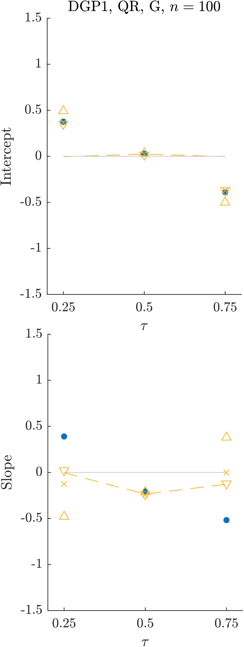
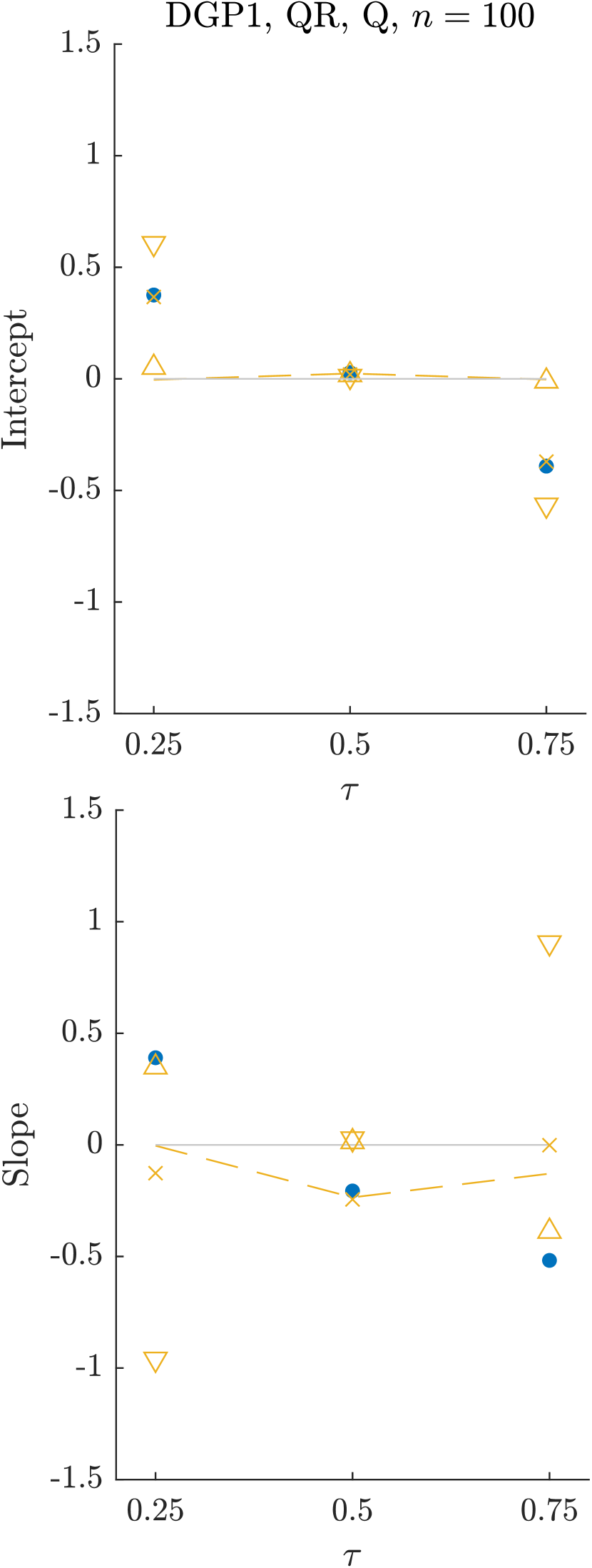
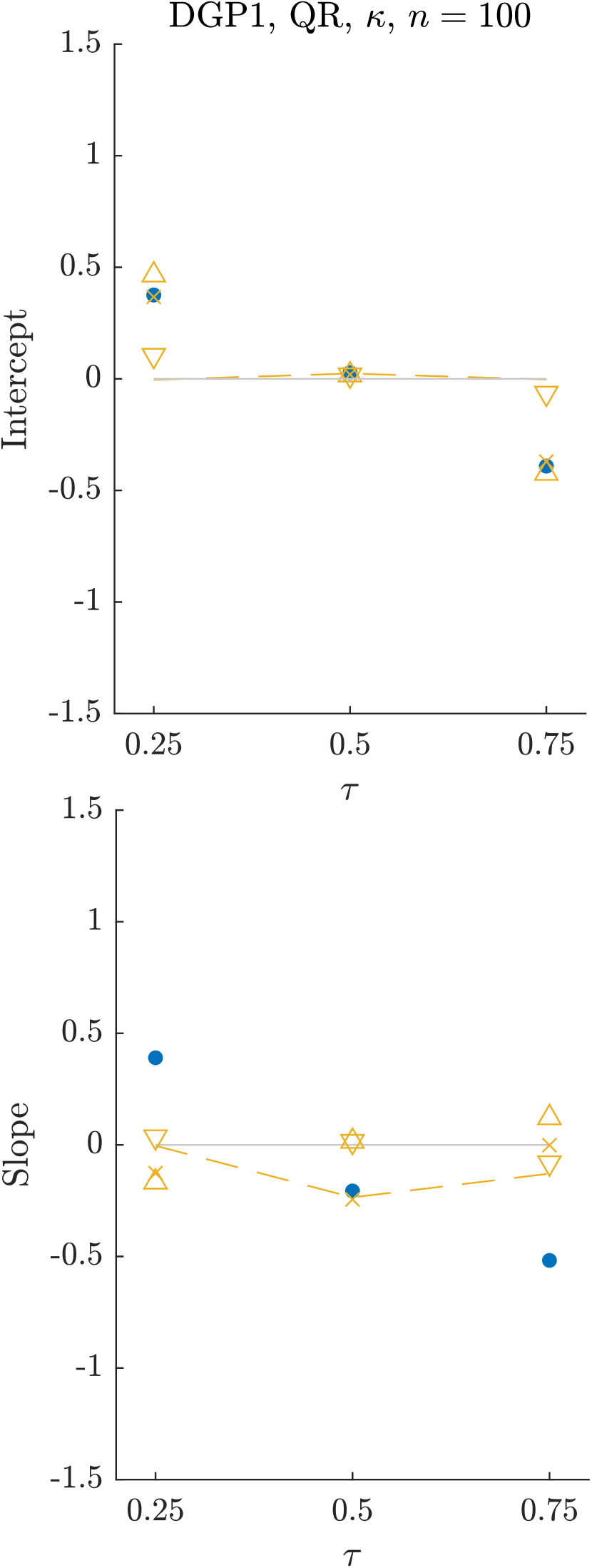
Notes: The panels display the bias (multiplied by $n$) of the intercept and the slope for classical QR without bias correction (blue dots), QR with feasible bias correction using the baseline bandwidth choice $A=(1,1,1)$ (gold crosses), QR with feasible bias correction using $\pm 0.5$ deviation in one bandwidth at a time (up-pointing triangles for $+0.5$, down-pointing triangles for $-0.5$), and QR with infeasible bias correction (gold dashed line) for DGP1. In Panel (a), we vary $A_{G}$, in Panel (b), we vary $A_{Q}$, and in Panel (c), we vary $A_{\kappa}$. All results are based on 40,000 simulation repetitions.

Figure 7: Mean absolute deviations (MAD) of raw and bias-corrected estimators

(a)

(b)

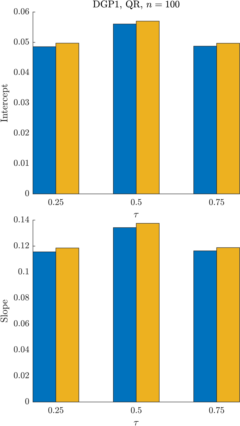
Notes: Panel (a) compares the MAD for classical QR without (blue) and with (gold) bias correction. Panel (b) compares the MAD for exact IVQR (implemented via the MILP formulation in Appendix D) without (blue) and with (gold) bias correction. The results for both DGPs are based on 40,000 simulation repetitions.

Figure 8: Confidence interval coverage before and after bias correction for DGP1, different sample sizes

(a)

(b)

(c)

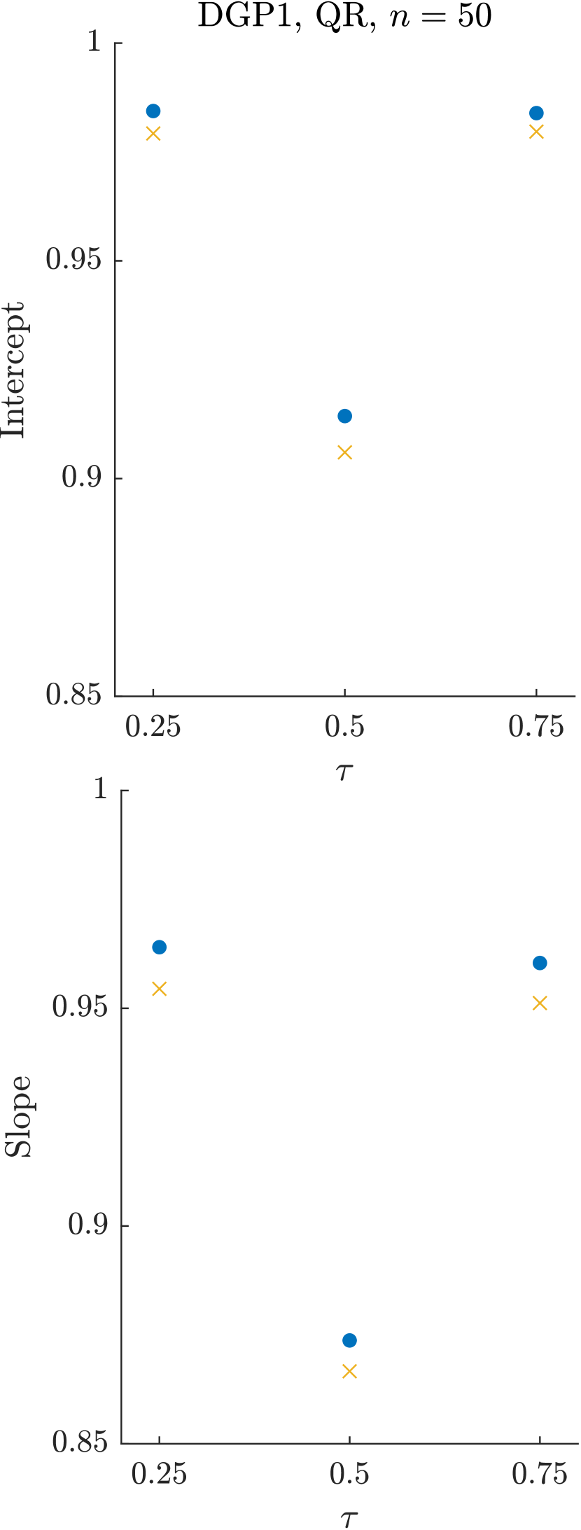
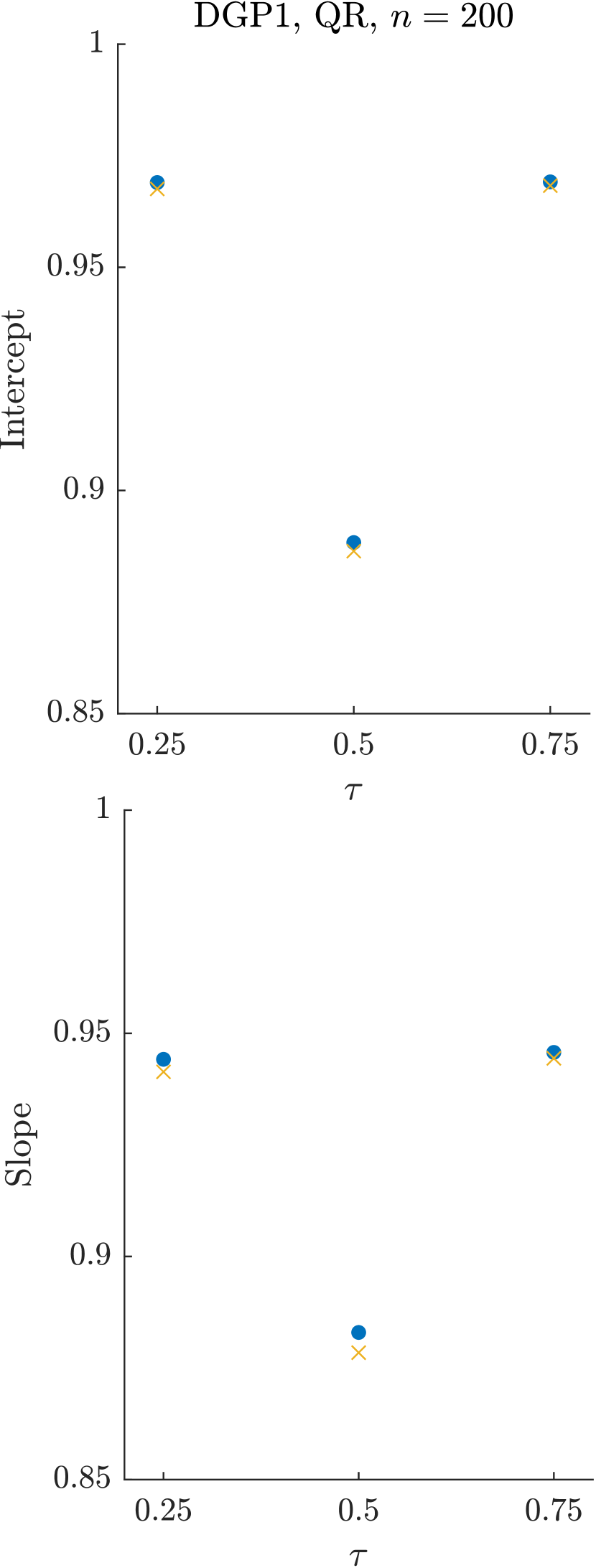
Notes: The panels display the coverage probability of the $90\%$ confidence intervals for the intercept and the slope for classical QR without bias correction (blue dots) and QR with the best feasible bias correction (gold crosses) for DGP1 with $n\in\{50,100,200\}$. All results are based on 40,000 simulation repetitions.

Figure 9: Confidence interval coverage before and after correction for DGP2–DGP4

(a)

(b)

(c)

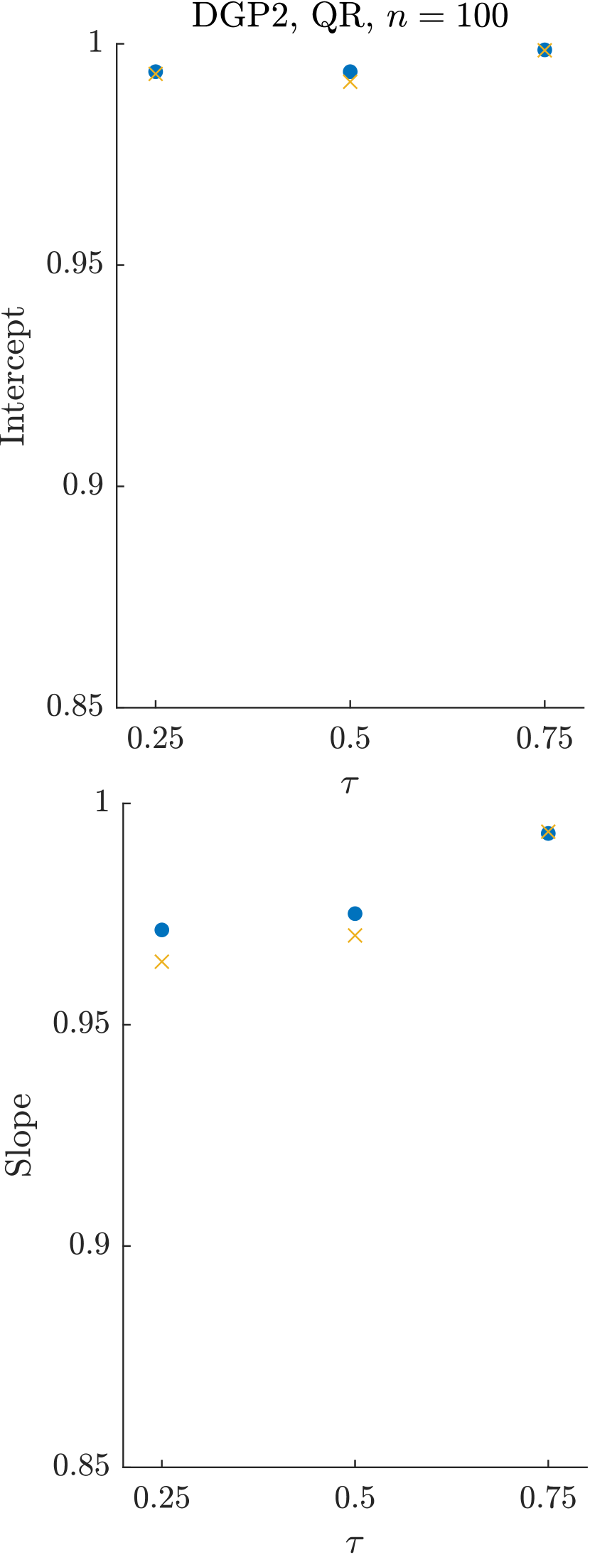
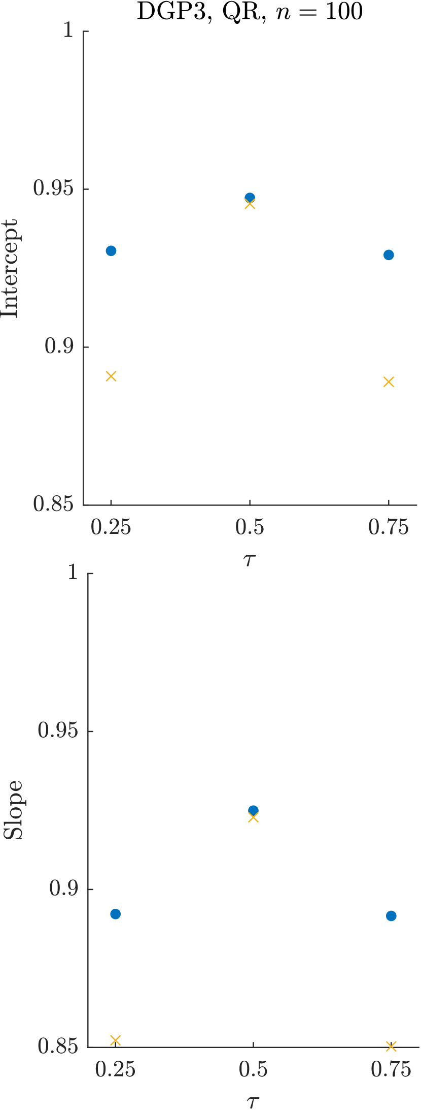
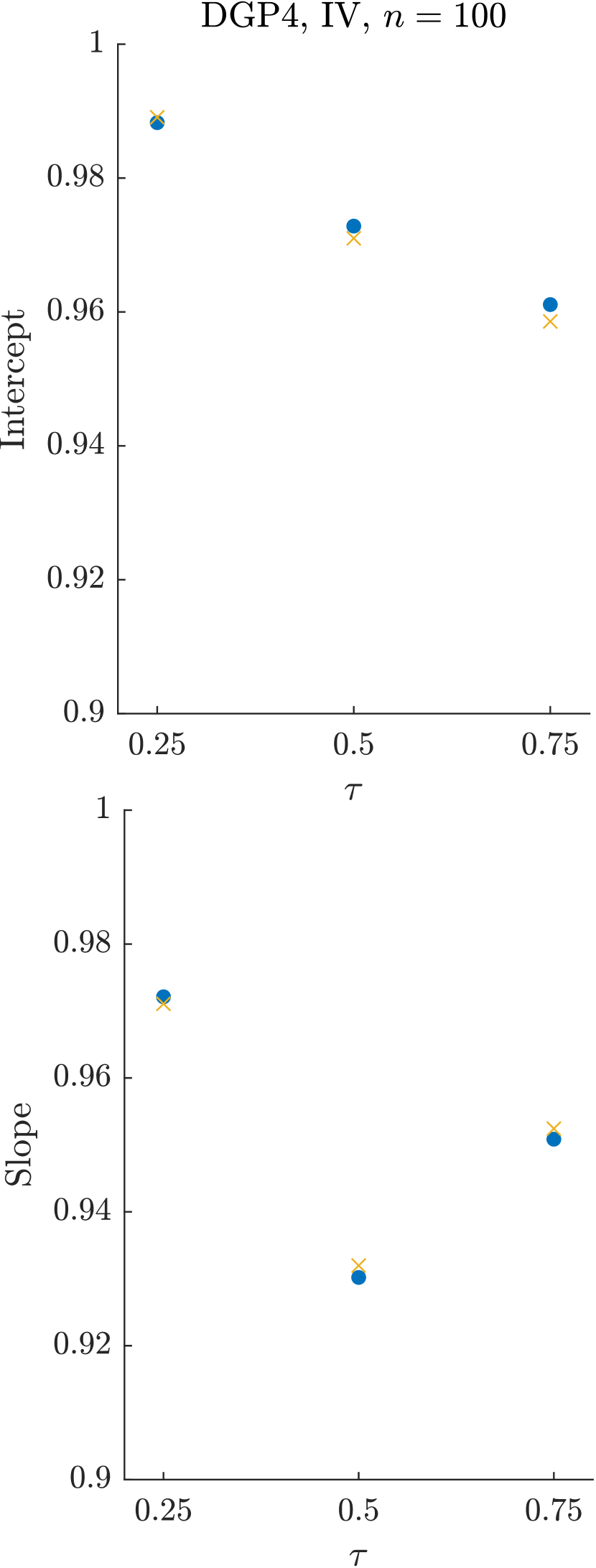
Notes: The panels display the coverage probability of the $90\%$ confidence intervals for the intercept and the slope for classical QR without bias correction (blue dots) and QR with the best feasible bias correction (gold crosses) for DGP2–DGP4 with $n=100$. All results are based on 40,000 simulation repetitions.

References

- Abramowitz and Stegun (1972) Abramowitz, M. and I. A. Stegun (1972): Handbook of Mathematical Functions with Formulas, Graphs, and Mathematical Tables, National Bureau of Standards Applied Mathematics Series 55. Tenth Printing.
- Adrian et al. (2019) Adrian, T., N. Boyarchenko, and D. Giannone (2019): “Vulnerable Growth,” American Economic Review, 109, 1263–89.
- Adrian and Brunnermeier (2016) Adrian, T. and M. K. Brunnermeier (2016): “CoVaR,” American Economic Review, 106, 1705–41.
- Ahsanullah et al. (2013) Ahsanullah, M., V. B. Nevzorov, and M. Shakil (2013): An introduction to order statistics, vol. 8, Springer.
- Andrews and Mikusheva (2016) Andrews, I. and A. Mikusheva (2016): “Conditional inference with a functional nuisance parameter,” Econometrica, 84, 1571–1612.
- Angrist et al. (2006) Angrist, J., V. Chernozhukov, and I. Fernández-Val (2006): “Quantile regression under misspecification, with an application to the US wage structure,” Econometrica, 74, 539–563.
- Chen and Lee (2018) Chen, L.-Y. and S. Lee (2018): “Exact computation of GMM estimators for instrumental variable quantile regression models,” Journal of Applied Econometrics, 33, 553–567.
- Chernozhukov (2005) Chernozhukov, V. (2005): “Extremal quantile regression,” The Annals of Statistics, 33, 806 – 839.
- Chernozhukov et al. (2014) Chernozhukov, V., D. Chetverikov, and K. Kato (2014): “Gaussian approximation of suprema of empirical processes,” The Annals of Statistics, 42, 1564–1597.
- Chernozhukov and Fernández-Val (2011) Chernozhukov, V. and I. Fernández-Val (2011): “Inference for extremal conditional quantile models, with an application to market and birthweight risks,” The Review of Economic Studies, 78, 559–589.
- Chernozhukov and Hansen (2005) Chernozhukov, V. and C. Hansen (2005): “An IV model of quantile treatment effects,” Econometrica, 73, 245–261.
- Chernozhukov and Hansen (2006) ——— (2006): “Instrumental quantile regression inference for structural and treatment effect models,” Journal of Econometrics, 132, 491–525.
- Chernozhukov and Hansen (2008) ——— (2008): “Instrumental variable quantile regression: A robust inference approach,” Journal of Econometrics, 142, 379–398.
- Elsner et al. (2008) Elsner, J. B., J. P. Kossin, and T. H. Jagger (2008): “The increasing intensity of the strongest tropical cyclones,” Nature, 455, 92–95.
- Engel (1857) Engel, E. (1857): “Die Produktions- und Konsumptionsverhältnisse des Königreichs Sachsen.” Zeitschrift des Statistischen Bureaus des Königlich Sächsischen Ministeriums des Innern, 8, 1–54.
- Galvao and Kato (2016) Galvao, A. F. and K. Kato (2016): “Smoothed quantile regression for panel data,” Journal of Econometrics, 193, 92–112.
- Hahn et al. (2023) Hahn, J., D. W. Hughes, G. Kuersteiner, and W. K. Newey (2023): “Efficient Bias Correction for Cross-section and Panel Data,” arXiv:2207.09943.
- Kaido and Wüthrich (2021) Kaido, H. and K. Wüthrich (2021): “Decentralization estimators for instrumental variable quantile regression models,” Quantitative Economics, 12, 443–475.
- Kallenberg (2006) Kallenberg, O. (2006): Foundations of modern probability, Springer Science & Business Media.
- Kaplan and Sun (2017) Kaplan, D. M. and Y. Sun (2017): “Smoothed estimating equations for instrumental variables quantile regression,” Econometric Theory, 33, 105–157.
- Kato (2012) Kato, K. (2012): “Asymptotic normality of Powell’s kernel estimator,” Annals of the Institute of Statistical Mathematics, 64, 255–273.
- Kato et al. (2012) Kato, K., A. F. Galvao Jr, and G. V. Montes-Rojas (2012): “Asymptotics for panel quantile regression models with individual effects,” Journal of Econometrics, 170, 76–91.
- Knight (2002) Knight, K. (2002): “Comparing conditional quantile estimators: first and second order considerations,” Working Paper.
- Koenker (2005) Koenker (2005): Quantile Regression, Cambridge University Press.
- Koenker (2022) Koenker, R. (2022): quantreg: Quantile Regression, R package version 5.94.
- Koenker and Bassett (1978) Koenker, R. and G. Bassett (1978): “Regression Quantiles,” Econometrica, 46, 33–50.
- Koenker and Bassett (1982) ——— (1982): “Robust Tests for Heteroscedasticity Based on Regression Quantiles,” Econometrica, 50, 43–61.
- Koenker and Hallock (2001) Koenker, R. and K. F. Hallock (2001): “Quantile Regression,” Journal of Economic Perspectives, 15, 143–156.
- Lee et al. (2017) Lee, T.-H., A. Ullah, and H. Wang (2017): “The Second-order Bias and MSE of Quantile Estimators,” Unpublished manuscript.
- Lee et al. (2018) ——— (2018): “The second-order bias of quantile estimators,” Economics Letters, 173, 143–147.
- Nagar (1959) Nagar, A. L. (1959): “The Bias and Moment Matrix of the General k-Class Estimators of the Parameters in Simultaneous Equations,” Econometrica, 27, 575–595.
- Newey and McFadden (1994) Newey, K. and D. McFadden (1994): “Large sample estimation and hypothesis,” Handbook of Econometrics, IV, Edited by RF Engle and DL McFadden, 2112–2245.
- Newey and Smith (2004) Newey, W. K. and R. J. Smith (2004): “Higher order properties of GMM and generalized empirical likelihood estimators,” Econometrica, 72, 219–255.
- Olver (2014) Olver, P. J. (2014): Introduction to partial differential equations, Springer.
- Ota et al. (2019) Ota, H., K. Kato, and S. Hara (2019): “Quantile regression approach to conditional mode estimation,” Electronic Journal of Statistics, 13, 3120–3160.
- Phillips (1991) Phillips, P. C. B. (1991): “A shortcut to LAD estimator asymptotics,” Econometric Theory, 450–463.
- Portnoy (2012) Portnoy, S. (2012): “Nearly root- approximation for regression quantile processes,” The Annals of Statistics, 40, 1714–1736.
- Powell (1986) Powell, J. L. (1986): “Censored regression quantiles,” Journal of Econometrics, 32, 143–155.
- Rilstone et al. (1996) Rilstone, P., V. Srivastava, and A. Ullah (1996): “The second-order bias and mean squared error of nonlinear estimators,” Journal of Econometrics, 75, 369 – 395.
- van der Vaart and Wellner (1996) van der Vaart, A. W. and J. A. Wellner (1996): Weak Convergence and Empirical Processes: With Applications to Statistics, Springer Science & Business Media.
- Vapnik and Chervonenkis (1971) Vapnik, V. N. and A. Y. Chervonenkis (1971): “On uniform convergence of the frequencies of events to their probabilities,” Teoriya Veroyatnostei i ee Primeneniya, 16, 264–279.
- Zhou and Portnoy (1996) Zhou, K. Q. and S. L. Portnoy (1996): “Direct use of regression quantiles to construct confidence sets in linear models,” The Annals of Statistics, 24, 287–306.
- Zhu (2019) Zhu, Y. (2019): “Learning non-smooth models: instrumental variable quantile regressions and related problems,” arXiv preprint arXiv:1805.06855.