Memory effects in glasses: insights into the thermodynamics of out of equilibrium systems revealed by a simple model of the Kovacs effect

Abstract

This paper is an extended version of an article accepted for publication in Physical Review E. Besides its fundamental interest, the model that we investigate in this article is simple enough to be used as a basis for courses or tutorials on the thermodynamics of out of equilibrium systems. It allows simple numerical calculations and analytical analysis which highlight important concepts with an easily workable example. This version includes studies of fast cooling and heating, exhibiting cases with negative heat capacity, and further discussions on the entropy which are not presented in the Physical Review E version.

Glasses are interesting materials because they allow us to explore the puzzling properties of out-of-equilibrium systems. One of them is the Kovacs effect in which a glass, brought to an out-of-equilibrium state in which all its thermodynamic variables are identical to those of an equilibrium state, nevertheless evolves, showing a hump in some global variable before the thermodynamic variables come back to their starting point. We show that a simple three-state system is sufficient to study this phenomenon using numerical integrations and exact analytical calculations. It also brings some light on the concept of fictive temperature, often used to extend standard thermodynamics to the out-of-equilibrium properties of glasses. We confirm that the concept of a unique fictive temperature is not valid, an show it can be extended to make a connection with the various relaxation processes in the system. The model also brings further insights on the thermodynamics of out-of-equilibrium systems. Moreover we show that the three-state model is able to describe various effects observed in glasses such as the asymmetric relaxation to equilibrium discussed by Kovacs, or the reverse crossover measured on $B_{2}O_{3}$.

I Introduction

Glasses are very common materials, and nevertheless they are very special, with fascinating properties which pose fundamental questions to physicists. When a glass is formed by cooling a liquid, the dynamics of molecular reorganization drastically slows down in a narrow temperature range, so that, below a temperature $T_{g}$, called the glass-transition temperature, or above some pressure $P_{g}$, the fluctuations within the material appear as frozen on observable time scales KOVACS . The mechanisms behind this transition are only partly understood BERTHIER2011 , but it is not the only question that glasses pose to theoreticians because, below $T_{g}$, they are out-of-equilibrium systems. Standard thermodynamics does not apply and this opens an entirely new world, with many puzzling properties. For instance experiments show that the heat capacity of a glass depends on its past history THOMAS1931 .

The Kovacs effects is another example which provides a revealing insight into the properties of out-of-equilibrium systems. Let us consider a glassy material, in the $V$, $T$ thermodynamic representation, that started from an initial equilibrium at temperature $T_{0}$ and was slowly cooled until it reaches a new equilibrium at a temperature $T_{1}$ with a specific volume $v(T_{1})$. Let us call this state state $A$. Then, in a second experiment the same piece of material is abruptly cooled from $T_{0}$ to a temperature $T_{2}<T_{1}$, $T_{2}$ being in the range of the glass transition temperature $T_{g}$. The material is let to age at $T_{2}$. Its specific volume is monitored while it slowly decreases with aging. When the specific volume reaches the value $v(T_{1})$ the material is quickly brought to temperature $T_{1}$. This new state, that we call state $B$, has now the same thermodynamic variables as state $A$, and we would therefore expect state $B$ to be in equilibrium. However, when state $B$ was kept at temperature $T_{1}$, Kovacs observed that its specific volume started to increase, then passed a maximum and decayed to reach the value $v(T_{1})$ again. Obviously state $B$ was not the same as state $A$ although both had the same thermodynamic equilibrium variables. This surprising experiment shows that the thermodynamic variables are not sufficient to characterize the state of out-of-equilibrium system such as a glass. There are further “hidden variables” which must also be specified. This idea brings two kinds of questions: i) what are the system features which can lead to such a situation, ii) what are its consequences and how do they affect the thermodynamic description of the system. The Kovacs effect has been widely studied with a particular attention on the first question BERTHIER2002 ; BERTIN ; AQUINO ; MOSSA . These studies consider various models which can exhibit glassy properties, with a distribution of length or time scales, and the coupling of many degrees of freedom, which can lead to memory effects. The second class of questions has been less explored. An article by Bouchbinder and Langer BOUCHBINDER examines the non-equilibrium thermodynamics of the Kovacs effect and lists the minimal ingredients for any model of this effect. However the view point that complexity is inherent to this phenomenon is suggested by the introductory sentence: “The Kovacs effect reveals some of the most subtle and important nonequilibrium features of glassy dynamics”. Actually, as we show here, the Kovacs effect exists in an extremely simple system, so simple that it may appear almost trivial. In spite of its simplicity, and perhaps because it is so simple, this model deserves a study because it allows a complete understanding of the mechanisms behind the Kovacs effect and brings a new light on the concept of fictive temperature DAVIESJONES widely used for glasses. It is now recognized that memory effects are not compatible with a unique fictive temperature LEUZZI . Our analysis confirms this view but moreover shows quantitatively why, and how the concept can be extended and generalized.

Besides its fundamental interest, the model that we investigate in this article is simple enough to be used as a basis for courses or tutorials on the thermodynamics of out of equilibrium systems. It allows simple numerical calculations and analytical analysis which highlight important concepts with an easily workable example.

Section II introduces the model, and discusses its relationship with an even simpler model which was used to illustrate non-equilibrium negative heat capacity in glasses. Section III shows how simple numerical integrations of this model exhibit the Kovacs effect. An analytical description is used in Sec. IV to recover the numerical results while providing a deeper understanding of the mechanisms behind these results and other unusual properties of glasses. Finally Sec. V examines to what extend these properties can be described by an extension of standard thermodynamics using the concept of “fictive temperature” DAVIESJONES , and how the out-of-equilibrium properties appear in the entropy, and entropy production, for the different processes studied with this model.

II Model

The glass transition can be observed for a large variety of systems, from liquids bonded by covalent, ionic or molecular forces, to granular materials or proteins. Therefore its microscopic description is not unique, but there is a unifying concept which underlies the various phenomena which are involved, the free energy landscape over which the system evolves. This highly multidimensional surface is itself very complex, but many properties of glasses can be derived from a reduced view, the inherent structure landscape which only describes the minima of the metastable states NAKAGAWA . This is enough to build a thermodynamics of the equilibrium properties of a glass, and, if the picture is completed by adding the barriers that have to be overcome to move between the minima, its dynamical properties can also be investigated. This idea can be pushed to the extreme by considering only a small number of energy states and the saddle points which separate one state from another.

The simplest model includes only two energy states, separated by one saddle point. This two-level system is sufficient to study the negative heat capacity observed in the vicinity of the glass transition, but, as shown below, it is nevertheless unable to describe other properties of glasses, such as the Kovacs effect. However, adding only one energy state, and two saddle points, as schematized on Fig. 1-a, is enough to illustrate fundamental ideas of the physics of out-of-equilibrium systems.

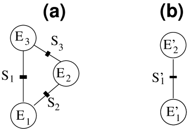
Figure 1: Picture of the three-state model (a) and its simplified version, the two-state model (b). The circles schematize the metastable states with energies $E_{i}$, and the thick lines the barriers that separate them, with energies $S_{i}$.

Let us denote by $E_{i}$ ($i=1,2,3$) the energies of the three metastable states. The probabilities $P_{i}$ that the states $i$ are occupied are the variables which define the state of the system. However, due to the constraint $P_{1}+P_{2}+P_{3}=1$, the state is actually defined by two parameters only. We henceforth select the two variables $P_{1}$ and $P_{2}$ to characterize a state of the system.

The equilibrium properties of the model are readily obtained from the Gibbs canonical distribution. Its partition function is

$$Z=\sum_{i}e^{-E_{i}/T}\;,$$ (1)

if we measure the temperature $T$ in energy units (which is equivalent to setting the Boltzmann constant to $k_{B}=1$). The occupation probabilities of the three states when the system is in equilibrium are

$$P_{i}^{\mathrm{eq}}=\frac{1}{Z}e^{-E_{i}/T}\;,$$ (2)

and the average energy of the system is

$$E^{\mathrm{eq}}(T)=\langle E(T)\rangle=\frac{1}{Z}\;\sum_{i}E_{i}e^{-E_{i}/T}\;.$$ (3)

Viewing this model as a simplified picture of the free energy landscape of a glass, we assume that the transitions from one basin of attraction to another are thermally activated over saddle points having energies $S_{1}$, for the transition between $E_{1}$ and $E_{3}$, $S_{2}$ for the transition between $E_{1}$ and $E_{2}$, and $S_{3}$ for the transition between $E_{2}$ and $E_{3}$. Therefore the transition probabilities are determined by a set barriers $B_{i,j}$, for instance $B_{1,3}=S_{1}-E_{1}$, $B_{3,1}=S_{1}-E_{3}$, $B_{1,2}=S_{2}-E_{1}$, and so on. The energies of the saddle points are assumed to be higher than the energies of the states that they separate so that $B_{i,j}>0$ for all $i,j$ pairs.

The rates of the thermally activated transitions are

$$W_{i\to j}=\omega_{ij}\;e^{-B_{ij}/T}$$ (4)

where $\omega_{ij}$ are model parameters which have the dimension of inverse time. As a result the thermodynamics of the model is expressed by equations for the time-dependence of the occupation probabilities, which are of the form

$$\frac{dP_{1}}{dt}= -P_{1}\,\omega_{13}\,e^{-(S_{1}-E_{1})/T}+P_{3}\,\omega_{31}\,e^{-(S_{1}-E_{3})/T}$$

$$-P_{1}\,\omega_{12}\,e^{-(S_{2}-E_{1})/T}+P_{2}\,\omega_{21}\,e^{-(S_{2}-E_{2})/T}\;,$$ (5)

and similar equations for $P_{2}$ and $P_{3}$.

For the equilibrium probabilities $P_{i}^{\mathrm{eq}}$, Eq. (II) becomes

$$\left(\frac{dP_{1}}{dt}\right)_{\mathrm{eq}}= -\frac{1}{Z}e^{-E_{1}/T}\,\omega_{13}\,e^{-(S_{1}-E_{1})/T}$$

$$+\frac{1}{Z}e^{-E_{3}/T}\,\omega_{31}\,e^{-(S_{1}-E_{3})/T}$$

$$-\frac{1}{Z}e^{-E_{1}/T}\,\omega_{12}\,e^{-(S_{2}-E_{1})/T}$$

$$+\frac{1}{Z}e^{-E_{2}/T}\,\omega_{21}\,e^{-(S_{2}-E_{2})/T}\;.$$ (6)

If we assume that $\omega_{13}=\omega_{31}$ the first two terms cancel each other, and if we assume that $\omega_{12}=\omega_{21}$, terms 3 and 4 cancel each other so that $(dP_{1}/dt)_{\mathrm{eq}}$ vanishes, as we expect for the equilibrium case. These conditions $\omega_{ij}=\omega_{ji}$ are the so-called “detailed balance” conditions, which ensure the existence of the equilibrium state. Detailed balance does not require $\omega_{13}=\omega_{12}$, however we shall henceforth assume

$$\omega_{ij}=1\qquad\forall i,j(i\not=j)\;.$$ (7)

Setting the common value of $\omega_{i,j}$ to $1$ defines the time unit (t.u.) for the system.

This model belongs to a class of systems described by a master equation which have been investigated in PradosJSTAT in a study which derived general properties of the Kovacs hump valid for a variety of systems. Instead our goal here is to show that a minimal model, for which an exact analytical analysis is straightforward, is able not only to generate the Kovacs effect but also other properties observed in real materials or complex models, as discussed in Sec. VI. Moreover we are also interested in the thermodynamics of out equilibrium systems (Sec. V). This model allows us to generalize the concept of fictive temperature, introduced in 1931 TOOL1931 and still widely used for glasses WONDRACZEK ; GUO-2011 but which fails for systems exhibiting the Kovacs effect.

III Numerical studies

Numerical integrations of Eq. (II), taking into account our choice (7) for $\omega_{i,j}$, provide a first insight of the properties of the model. We selected the following parameters. The energy level $E_{3}$ has been used as the reference level for the energies by setting $E_{3}=0$. The energies of the two other states were chosen as $E_{1}=-0.40$ and $E_{2}=-0.25$. The energies of the saddle points were set to $S_{1}=0.40$, $S_{2}=0.30$, $S_{3}=0.25$. As the model does not intend to describe a specific glass, the energy scale is irrelevant and the values have been chosen arbitrarily. Other choices would of course quantitatively modify the results but, as long as the conditions $B_{ij}>0$ are verified and the ratios of the investigated temperatures and energies stay in the same range, the main features of the results would be preserved.

Figure 2: Equilibrium properties of the model: energy (full lines) and heat capacity (dashed lines) versus temperature. The thick lines show the results for the three-state model, and the thin lines show the results for the two-state model for comparison.

Figure 2 shows the equilibrium energy and heat capacity versus temperature for the three-state model of Fig. 1-a. For comparison it also shows the same quantities for the two-state model of Fig. 1-b, with the parameters $E^{\prime}_{1}=-0.40$, $E^{\prime}_{2}=0$, and $S^{\prime}_{1}=0.40$ chosen so that this restricted model simply corresponds to the three-state model without the intermediate state $E_{2}$. The two models have qualitatively similar equilibrium properties.

In a typical experiment, the system is in equilibrium at a temperature $T_{\mathrm{ini}}$ at time $t=0$. Then its temperature is varied by choosing a series of set-points $T^{s}_{j}$ and defining the time points $t_{j}$ at which each set-point has to be reached. This defines a trajectory $T(t)$ which is imposed to the system while its state variables $P_{i}(t)$ are followed. The evolution of the system is defined by Eq. (II) and the corresponding equations for $P_{2}(t)$ and $P_{3}(t)$, with constrained values for $T(t)$ in the right hand sides. The initial values of the state variables are the values $P_{i}^{\mathrm{eq}}(T_{\mathrm{ini}})$ which are known since they are given by Eq. (2). Any standard algorithm can be used to solve the set of three coupled equations for $P_{1}$, $P_{2}$, $P_{3}$. In our calculations we used the $4^{\mathrm{th}}$-order Runge-Kutta method CARNAHAN . The time step $\delta t$ can be chosen according to the characteristic relaxation times of the system (see. Sec. IV), however, as the integration only involves the solution of three coupled differential equations, choosing a small value such as $\delta t=0.01$ ensures a high accuracy without a significant computational cost. As the system only has two independent variables, $P_{1}$ and $P_{2}$, the computation could be simplified by solving only two coupled equations, completed by the condition $P_{3}=1-(P_{1}+P_{2})$. However, solving the three coupled equations is interesting because it allows a simple test of accuracy, and a check of the value of $\delta t$, by making sure that the condition $\sum P_{i}=1$ is well preserved by the calculation.

III.1 Fast cooling and heating

As a first example of the properties of the three-state model, let us consider a first simulated experiment involving a simple cooling at fixed cooling rate, followed by heating at the same rate. The temperature set-points are $T_{\mathrm{ini}}=0.20$, $T^{s}_{1}=0.02$ at time $t_{1}=10^{4}\;$t.u. , $T^{s}_{2}=0.20$ at $t_{2}=2\;10^{4}\;$t.u. .

(a)

(b)

Figure 3: Energy (a) and heat capacity (b) versus temperature when the three-state system is cooled from $T_{\mathrm{ini}}=0.20$ to $T^{s}_{1}=0.02$ in $t_{1}=10^{4}$ time units, with a constant cooling rate, and then heated again from the final state back to $T^{s}_{2}=0.20$ in the same time interval. The thin full lines show the properties of the model upon cooling, while the full thick black lines show its behavior upon heating. The dashed lines show the equilibrium properties of the model versus temperature.

Figure 3-a shows the variation of the total energy of the system versus temperature. On cooling, it shows that, above $T\approx 0.1$ the energy (thin full line) follows the curve of the equilibrium energy versus $T$ (dashed line). But when the temperature decreases further, the energy starts to decay more slowly than the equilibrium energy and stays almost constant when $T<0.05$. The temperature range $0.05<T<0.10$ is the domain of the glass transition, below which the dynamics of the system tends to freeze. The large deviation between the observed value of the energy of the system after cooling and the equilibrium energy at the same temperature, shows that, with the cooling rate that we used for this simulation, the system was brought to a strongly out-of-equilibrium state. If the simulation is repeated with a larger value of $t_{1}$, i.e. with a smaller cooling rate, the energy follows the equilibrium energy down to lower temperatures, as expected since we gave the system a longer time to approach equilibrium.

When the system is heated from the state that it reached after cooling, the energy (full thick curve) stays constant and even slightly decreases in the temperature range of the glass transition and passes below the curve of the equilibrium energy versus temperature, before rising sharply to join the curve of the equilibrium energy. Figure 3-b, showing the heat capacity $C=dE/dT$ emphasizes this behavior. The heat capacity versus temperature has the characteristic shape observed when a glassy material is heated after a rapid cooling THOMAS1931 , with a hump after a sharp rise before it reaches the equilibrium heat capacity at high temperature. In this case, as cooling was fast enough to bring the system very far from equilibrium, the fast rise is preceded by domains in which the heat capacity is negative, a phenomenon often observed in calorimetric heating scans through the glass transition DEBOLT . This simulation shows that the three-state system can exhibit the typical properties of a glassy system. This kind of behavior was also observed for the simpler two-state system of Fig. 1-b BISQUERT ; JABRAOUI . However, to explore more subtle glassy properties, such as the Kovacs effect, the three states are necessary.

Kovacs effect

The Kovacs effect is observed when one follows some property, such as the specific volume, of a glassy material subjected to a particular protocol. For the three-state system the volume has no meaning but we can follow another variable, such as the energy $E=\sum P_{i}E_{i}$. We do not need to perform the preliminary scan with a slow cooling mentioned in the introduction because we know the equilibrium energy $E^{\mathrm{eq}}(T)$ from Eq. (3). Let us consider the following thermal protocol $T(t)$: we start from an equilibrium state at $T^{\mathrm{ini}}=0.30$. At time $t=0$ the system is abruptly cooled to $T_{1}=0.02$ and we let it age at this temperature until $t_{1}=1.8\,10^{7}$t.u. . At the end of this aging period its energy has decreased to a value $E_{1}$. We determine the temperature $T_{2}$ at which this energy would be the equilibrium energy by solving the equation $E^{\mathrm{eq}}(T_{2})=E_{1}$, which gives $T_{2}=0.17856$. At this instant $t_{1}$, the temperature of the system is brought to $T_{2}$ and we follow its evolution for $10^{4}$t.u. . As its energy corresponds to the equilibrium energy $E^{\mathrm{eq}}(T_{2})$, we could expect that nothing happens and that the system simply stays in equilibrium. As shown by Fig. 4-a, this is not what is observed.

(a)

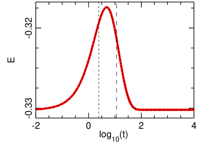
(b)

Figure 4: Energy (a) and probabilities $P_{1}$,$P_{2}$, $P_{3}$ (b) versus time (in log scale) during the time evolution at constant temperature $T_{2}=0.17856$ after aging for $1.8\,10^{7}\,$t.u. at temperature $T_{1}=0.02$ in the study of the Kovacs effects. In plot (a), the thick red line shows the numerical result and the short-dash line shows the result of the theoretical calculation (Sec. IV). Plot (b): full line $P_{1}$, short-dash line $P_{2}$, long-dash line $P_{3}$. The points at the right side of the graph show the values of the equilibrium probabilities at $T_{2}$ : circle $P_{1}^{\mathrm{eq}}$, square $P_{2}^{\mathrm{eq}}$, star $P_{3}^{\mathrm{eq}}$. In both plots, the vertical lines mark the relaxation times (short-dash line $\tau_{1}$, long-dash line $\tau_{2}$).

The energy starts to grow, shows a hump, and decays back to its original value. This is exactly what Kovacs observed for the volume of a vinyl polyacetate sample, with a similar protocol KOVACS . Figure 4-b helps to understand what happens. It shows that, at the end of the aging period, when temperature was abruptly raised to $T_{2}$, the occupation probabilities $P_{i}$ of the tree states were very different from the equilibrium probabilities $P_{i}^{\mathrm{eq}}(T_{2})$. Although the energy of the system was $E_{1}=E^{\mathrm{eq}}(T_{2})$, the system was not in the equilibrium state at $T_{2}$. This is possible because the three-state system has two internal degrees of freedom $P_{1}$, $P_{2}$. A given value of its energy $E=P_{1}E_{1}+P_{2}E_{2}+[1-(P_{1}+P_{2})]E_{3}$ can be realized by different microscopic states, characterized by $P_{1}$ and $P_{2}$. If the system is prepared in a non-equilibrium state by a specific protocol (a temperature quench followed by aging at low temperature in Kovacs experiment) then the internal degrees of freedom do not have their equilibrium values. In the time evolution at temperature $T_{2}$ the internal variables evolve towards equilibrium. As shown by the theoretical analysis of Sec. IV, this process is a relaxation, which does not guarantee that $E$ should stay constant. And actually it does not, and we observe the hump characteristic of the Kovacs effect.

The scheme that we described above appears to be very general. A macroscopic system has many internal degrees of freedom, and therefore many internal configurations which could lead to the same energy (or the same specific volume, for the variable studied in Kovacs experiment). So, why don’t we observe the Kovacs effects for almost any material. The answer lies in the possibility to prepare the system in an adequate out-of-equilibrium state. Usually the time scale at which the internal variables approach equilibrium is too fast to allow us to observe the Kovacs effect. This is different for glasses which are material in which some degrees of freedom are almost frozen or at least evolve so slowly that we can follow their evolution. In the experiment of Kovacs, the characteristic time of this evolution was of the order of several hundreds hours.

What we have described here for the three-state system cannot be observed for the two-state system. If a calculation is carried with the same protocol for the two-state system, when the temperature is kept constant at $T_{2}$ after aging, the energy stays strictly constant. The Kovacs hump is not observed with this model. It is easy to understand why. The two state-system only has one degree of freedom. Its energy is $E=P_{1}E_{1}+[1-P_{1}]E_{2}$. There is a one-to-one correspondence between $E$ and $P_{1}$. Therefore looking for $T_{2}$ by solving $E_{1}=E^{\mathrm{eq}}(T_{2})$ is equivalent to solving $P_{1}=P_{1}^{\mathrm{eq}}(T_{2})$, i.e., when we start the time evolution at $T_{2}$, the system is already in its equilibrium state. Some studies have reported the Kovacs effects in models based on two-state systems PradosJSTAT ; AQUINO2008 , but these models also include disorder, either through dynamic fluctuations of the height of the barrier between the states, or through a distribution of model parameters. This extends the configuration space of the model so that the energy of the system does not fully determine the configuration of the system.

To make sure that we do observe the Kovacs effect, it is necessary to check that the numerical results obtained with the three-state system match the various experimental features of this effect. Besides the existence of the Kovacs humps, experiments show that the hump gets smaller, and appears at a later time when the difference between the temperature $T_{1}$ of the aging period and that of the Kovacs time evolution at $T_{2}$ decreases. Starting from the same initial equilibrium at $T^{\mathrm{ini}}=0.30$ we have performed calculations for different values of the aging temperature $T_{1}$, $T_{1}=0.030,\;0.032,\;0.033$ with the same aging time $t_{1}=1.8\,10^{7}$t.u. . The final energy $E_{1}$ depends on $T_{1}$ and therefore the temperature $T_{2}$ such that $E_{1}=E^{\mathrm{eq}}(T_{2})$ also changes. Figure 5 shows that the hump depends on $\Delta T=T_{2}-T_{1}$ as observed by Kovacs KOVACS . For the three-state system this behavior can be justified analytically as discussed in Sec. IV.

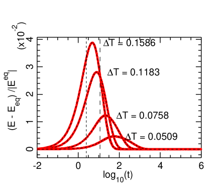
Figure 5: Normalized Kovacs hump $(E-E^{\mathrm{eq}})/|E^{\mathrm{eq}}|$ versus time (in log scale) for various values of the temperature jump $\Delta T=T_{2}-T_{1}$. The thick red lines are the results of the numerical integrations and the black dashed lines are analytical calculations (Sec. IV).

IV Analytical analysis

A configuration of the three-state system depends on the two variables $P_{1}$ and $P_{2}$. Their variation versus time could be obtained by numerical integrations, but, as Eq. (II) and the corresponding equation for $P_{2}$ are a set of coupled first order linear differential equations, they can also be solved analytically.

It is convenient to introduce the deviations with respect to equilibrium $Q_{i}=P_{i}-P_{i}^{eq}$. The condition $P_{1}+P_{2}+P_{3}=1$ results in $Q_{1}+Q_{2}+Q_{3}=0$. Note that there is no assumption regarding the size of $Q_{i}$ compared to $P_{i}^{eq}$, i.e. this change of variable does not imply any small amplitude expansion. Actually when the system is subjected to an abrupt temperature change, immediately after the temperature jump the $P_{i}$ have preserved their values while the $P_{i}^{eq}$ have drastically changed. This may lead to situations where $|Q_{i}/P_{i}|\gg 1$.

As shown in Appendix A, the solution of the system of linear equations for $Q_{1}$, $Q_{2}$ can be expressed in terms of two eigenmodes as

$$\vec{Q}=a(t)\vec{U}^{(1)}+b(t)\vec{U}^{(2)}\;.$$ (8)

where $\vec{U}^{(1)}$ and $\vec{U}^{(2)}$ are two eigenvectors and $a(t)$, $b(t)$, the amplitudes of the modes, are given by two exponential relaxations

$$a(t) =a(t=0)\exp[-t/\tau_{1}]$$

$$b(t) =b(t=0)\exp[-t/\tau_{2}]\;,$$ (9)

characterized by two relaxation times $\tau_{1}$, $\tau_{2}$. Both the eigenvectors and the relaxation times depend on the parameters of the model and on temperature. For any constant-temperature process the modes are well defined and the time dependencies of their amplitudes are readily obtained from their values at the beginning of the evolution period, which are themselves determined from the initial values of the probabilities $P_{i}(t=0)$ through the definition of the $Q_{i}$s and Eq. (8). For a protocol starting from an equilibrium state, and comprising only temperature jumps, during which the probabilities $P_{i}$ do not change, and time evolutions at constant temperature this provides a systematic procedure to derive an exact analytical solution which determines the complete evolution of the system.

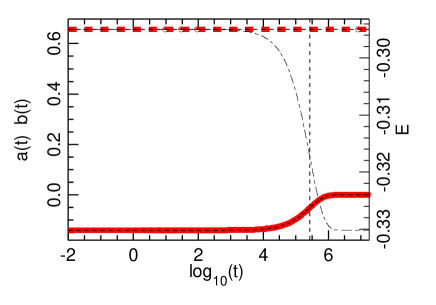
Figure 6: Amplitudes of the eigenmodes $a(t)$ and $b(t)$ during the aging stage at temperature $T_{1}$ in the protocol to observe the Kovacs effect. The thick red lines sow the results of the numerical integration with a full line for $a(t)$ and a dash line for $b(t)$. The short-dash black lines are the results of the analytical calculation. The vertical short-dash line marks the value of $\tau_{1}(T_{1})$. The thin dash-dot line shows the variation of the energy (right scale).

Besides providing an analytical method to study the out-of-equilibrium properties of a system, the decomposition of the dynamics on the normal modes brings further understanding of the observations. This is clear for the protocol used to study the Kovacs effect. We start from an equilibrium state at $T^{\mathrm{ini}}=0.30$ and therefore at $t=0$ the probabilities are $P_{i}(t=0)=P_{i}^{\mathrm{eq}}(T^{\mathrm{ini}})$. At this time the temperature is switched to $T_{1}=0.02$. Solving Eq. (39) we can determine the eigenvalues $\lambda_{1,2}(T_{1})$, i.e. the relaxation times $\tau_{1,2}(T_{1})=-1/\lambda_{1,2}(T_{1})$ and the eigenvectors $\vec{U}^{(1)}(T_{1})$, $\vec{U}^{(2)}(T_{1})$. This gives $\tau_{1}(T_{1})=0.2682\,10^{6}$t.u. and $\tau_{2}(T_{1})=0.8708\,10^{12}$t.u. . Solving Eq. (8) for the initial condition $Q_{i}(t=0)=P_{i}(t=0)-P_{i}^{\mathrm{eq}}(T_{1})$ we compute $a(t=0)$, $b(t=0)$, and then Eq. (IV) gives $a(t)$ and $b(t)$ at any time up to the end of the aging period $t=t_{1}$. Figure 6 shows that the analytical calculation perfectly agrees with the numerical integration, but it also helps us understand what happens during the aging stage. Mode 1 i.e. $a(t)$, which turns out to be negative, relaxes towards $0$ during aging, with the characteristic time $\tau_{1}$. Note that, if the exponential relaxation of $a$ appears like a step, it is due to logarithmic scale used for time on the horizontal axis. As $t_{1}=1.8\,10^{7}\ll\tau_{2}$ the amplitude $b(t)$ does not show any noticeable change during aging. As shown by Fig. 6 the relaxation of $a(t)$ is associated to a significant energy drop. However as the aging time was much shorter than $\tau_{2}$, the system has not reached equilibrium at the end of aging.

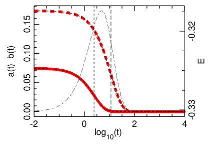
Figure 7: Amplitudes of the eigenmodes $a(t)$ and $b(t)$ during the constant temperature time evolution at temperature $T_{2}$ in the protocol to observe the Kovacs effect. The thin dash-dot line shows the variation of the energy (right scale). It reproduces the result already shown in Fig; 4-a, which can now be understood in terms of normal modes. The thick red lines sow the results of the numerical integration with a full line for $a(t)$ and a long-dash line for $b(t)$. The short-dash black lines are the results of the analytical calculation. The vertical lines marks the values of $\tau_{1}(T_{2})$ (short-dash line) and $\tau_{2}(T_{2})$ (long-dash line).

The analytical calculation gives the value of $a(t_{1})$, $b(t_{1})$ at the end of the aging stage of the Kovacs protocol. Therefore we know the probabilities $P_{i}(t_{1})$, from which we can deduce the values $Q_{i}(t_{1}^{+})$ of the deviations with respect to $P_{i}^{\mathrm{eq}}(T_{2})$ at the beginning of the last stage of the Kovacs protocol, which is designated as $t_{1}^{+}$, to point out that we consider this point as the start point of the next stage. Projecting the $Q_{i}(t_{1}^{+})$ on the normal modes at temperature $T_{2}$ we get the initial values $a_{0}(t_{1}^{+})$, $b_{0}(t_{1}^{+})$ of the amplitudes of the eigenmodes at the beginning of this last stage, and we obtain $a(t)$, $b(t)$ for the full duration of the Kovacs stage, which gives us the probabilities and the energy during this stage. This allows a full analytical calculation of the Kovacs effect in the three-state model, but, as for the relaxation to equilibrium discussed above, it also provides a quantitative understanding of the properties of the Kovacs hump. Figure 7 shows that the hump occurs because the two modes relax at different time scales. The relaxation times at temperature $T_{2}$ are $\tau_{1}=2.471\;$t.u. and $\tau_{2}=11.59\;$t.u. . They differ by many orders of magnitude from the relaxation times during aging. This is typical for a process taking place in the vicinity of a glass transition, as in the experiments of Kovacs. The rise of the Kovacs hump is observed when mode 1 relaxes, and the drop of the hump is due to the relaxation of mode 2. Therefore the properties of the Kovacs hump, shown in Fig. 5 can be quantitatively explained in terms of the eigenmodes of the three-state system. When $\Delta T=T_{2}-T_{1}$ decreases, i.e. $T_{2}$ decreases towards the low temperature $T_{1}$ for which the relaxation times become very long, the Kovacs hump moves later in time. Moreover, when the temperature decreases, the ratio $\tau_{2}/\tau_{1}$ increases. This explains why the hump becomes broader. The decay of its amplitude is also easy to understand qualitatively. When $T_{2}$ gets closer to $T_{1}$ the probabilities $P_{i}^{\mathrm{eq}}(T_{2})$ are closer to $P_{i}^{\mathrm{eq}}(T_{1})$, which leads to smaller values of $Q_{i}(t_{1}^{+})$. Then the $a_{0}(t_{1}^{+})$, $b_{0}(t_{1}^{+})$ are smaller, so that the relaxation of the two modes, which generates the Kovacs hump, is weaker.

V Extending thermodynamics to out-of-equilibrium systems ?

V.1 Fictive temperature

The concept of fictive temperature $T_{f}$, introduced by Tool and Eichling TOOL1931 assumes that any state of an out-of-equilibrium system at temperature $T$ is identical to an equilibrium state at another temperature $T_{f}$. This is a powerful concept which has been widely used to study glasses WONDRACZEK ; GUO-2011 ; VALLE-2012 , however it has some limitations RITLAND ; LEUZZI . This idea implies that an out-of-equilibrium system can be fully described by a set of thermodynamic variables at equilibrium, and, as discussed in the introduction, this is not compatible with the existence of the Kovacs effect. In the Kovacs protocol, at the end of the aging stage, when energy has reached the value $E_{1}$ we look for a temperature $T_{2}$ such that $E^{\mathrm{eq}}(T_{2})=E_{1}$. Using the concept of fictive temperature, it means that $T_{2}=T_{f}$ so that the state reached at the end of aging should be identical to the equilibrium state at temperature $T_{2}$. The experimental Kovacs hump, as well as its analysis within the three-state system discussed above, show that it is not true.

To understand the origin of this difficulty with the concept of $T_{f}$, it is necessary to come back to the fundamental definition of temperature in thermodynamics, expressed by the standard formula $dS=\delta Q/T$, relating the entropy $S$ and the heat exchange $\delta Q$ in an infinitesimal transformation occurring at equilibrium. For an out-of-equilibrium process, $1/T$ is no longer an integrating factor which can turn the heat exchange $\delta Q$ into an exact differential form because $\delta Q/T$ depends on the pathway in the configuration space, as shown by the Clausius inequality for a cycle. Nevertheless one can define a fictive temperature $T_{f}^{S}$ which plays the role of such an integrating factor by extending the usual definition of temperature so that the integration of $\delta Q/T_{f}^{S}$ along a temperature cycle vanishes whatever the thermodynamic path in the configuration space, i.e. whatever the thermal history of the system along the cycle. For a system such as the three-state system the heat exchange is merely equal to the variation of its energy, so that the fictive temperature should be defined by

$$\frac{1}{T_{f}^{S}}=\frac{\partial S}{\partial E}\;.$$ (10)

Consequently, when the system undergoes an infinitesimal transformation in which the probabilities $P_{i}$ change by $dP_{i}$, from the expression of the energy $E=\sum P_{i}\,E_{i}$ and the statistical expression of the entropy $S=-\sum P_{i}\;\ln P_{i}$ (with $k_{B}=1$ because we express temperatures in energy units), we get

$$T_{f}^{S}=-\;\frac{\sum_{i=1}^{N}E_{i}\;dP_{i}}{\sum_{i=1}^{N}\ln P_{i}\;dP_{i}}\;.$$ (11)

In the particular case of the three-state system with $P_{3}=1-P_{1}-P_{2}$, this leads to

$$T_{f}^{S}=-\;\frac{(E_{1}-E_{3})dP_{1}+(E_{2}-E_{3})dP_{2}}{dP_{1}\ln\left(\frac{P_{1}}{P_{3}}\right)+dP_{2}\ln\left(\frac{P_{2}}{P_{3}}\right)}$$ (12)

For the three-state system, $P_{1}$ and $P_{2}$ are independent variables, so that $dP_{1}$, $dP_{2}$ are arbitrary. Therefore Eq. (12) shows that the value of $T_{f}^{S}$ cannot be defined in term of the microscopic variables $P_{1}$, $P_{2}$. It also depends on the particular infinitesimal transform which is considered, i.e. on the path that the system follows in its parameter space $P_{1}$, $P_{2}$. Let us label $T_{f}^{S,\mathrm{transfo}}$ this value of the fictive temperature to stress that is is only meaningful for a particular transformation.

When the system approaches equilibrium, the occupation probabilities $P_{i}$ tend to $P_{i}=(1/Z)\exp(-E_{i}/T)$ and therefore the denominator of $T_{f}^{S}$ in Eq. (12) tends towards $\left[(E_{3}-E_{1})dP_{1}+(E_{3}-E_{2})dP_{2}\right]/T$ so that the expression of $T_{f}^{S}$ simplifies and tends to $T$, independently of $dP_{1}$, $dP_{2}$, i.e. whatever the path used to approach equilibrium, as expected for a fictive temperature.

While $T_{f}^{S}$ cannot be uniquely defined from the instantaneous state of a glassy system out of equilibrium, it is nevertheless possible to define fictive temperatures which have an intrinsic meaning. As we can define fictive temperatures associated to particular transformations, it is interesting to consider the transformations associated to the eigenmodes. At fixed temperature we have $dP_{i}=dQ_{i}$ because the equilibrium probabilities are constant. Moreover the time dependence of the $Q_{i}$s is related to the eigenmodes by Eqs (8) and (IV) i.e.

$$Q_{1} =a_{0}e^{-t/\tau_{1}}U_{1}^{(1)}+b_{0}e^{-t/\tau_{2}}U_{1}^{(2)}$$

$$Q_{2} =a_{0}e^{-t/\tau_{1}}U_{2}^{(1)}+b_{0}e^{-t/\tau_{2}}U_{2}^{(2)}\;.$$ (13)

Therefore, if only mode 1 is excited ($b_{0}=0$), for a time step $dt$ we have

$$\frac{dQ_{1}}{dQ_{2}}=\frac{dP_{1}}{dP_{2}}=\frac{U_{1}^{(1)}}{U_{2}^{(1)}}\;.$$ (14)

(Remember that $dP_{i}=dQ_{i}$.) The fictive temperature $T_{f}^{S}$ associated to this transformation, that we denote $T_{f}^{S,1}$ because it corresponds to a transformation in which mode 1 only is activated, is equal to

$$T_{f}^{S,1}=-\frac{(E_{1}-E_{3})U_{1}^{(1)}+(E_{2}-E_{3})U_{2}^{(1)}}{U_{1}^{(1)}\ln\left(\frac{P_{1}}{P_{3}}\right)+U_{2}^{(1)}\ln\left(\frac{P_{2}}{P_{3}}\right)}\;.$$ (15)

A similar formula, involving the components $U_{1}^{(2)}$, $U_{2}^{(2)}$ of the eigenvector of mode 2 defines $T_{f}^{S,2}$ for a transformation involving mode 2 only, starting from the state $P_{1}$, $P_{2}$.

Therefore, for any time evolution of the system, for each state $P_{1}$, $P_{2}$ we can define two fictive temperatures $T_{f}^{S,1}$, $T_{f}^{S,2}$ which tell us how far the system is from its actual temperature $T$ regarding one particular mode, i.e. regarding one particular relaxation time.

(a)

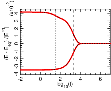
(b)

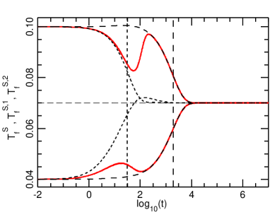
Figure 8: Approach to equilibrium: the temperature of the three-state system in equilibrium at $T=0.10$ or $T=0.04$ was abruptly switched to $T=0.07$ and we followed the evolution of the system for $10^{7}\;$t.u. . (a): Evolution of the energy of the system versus time. The figure shows the deviation of the energy $E(t)$ from the equilibrium energy $E^{\mathrm{eq}}$ at $T=0.07$ divided by $E^{\mathrm{eq}}$. The thick red lines are the numerical results. The thin black lines superimposed to them are the results of analytical calculations using the expansion on the eigenmodes. (b) Fictive temperatures during approach to equilibrium from above and from below. Red full line: $T_{f}^{S,\mathrm{transfo}}$ computed along the thermodynamic trajectory. Short-dash and long-dash black curves: $T_{f}^{S,1}$ and $T_{f}^{S,2}$, the fictive temperatures relative to the two eigenmodes. On both panels the vertical lines mark the relaxation times of the modes $\tau_{1}$ (short dash) and $\tau_{2}$ (long dash) at thermostat temperature $T$ marked by the thin dashed horizontal line.

As a first example let us study another characteristic feature of glasses, which was exhibited by Kovacs in his pioneering work KOVACS , the asymmetry of the kinetics of the approach to equilibrium upon cooling versus heating in the range of the glass transition. Figure 8 shows the behavior of the three-state model when it approaches equilibrium at $T=0.07$ both on cooling from an equilibrium state at $T=0.10$ and on heating from $T=0.04$. In each case, the temperature is abruptly changed from the initial temperature to $T=0.07$. Figure 8-a shows the evolution of the deviation of the energy $E(t)$ from the equilibrium energy $E^{\mathrm{eq}}$ at $T=0.07$. The variations on cooling and on heating are not symmetric, with an energy change starting earlier on cooling than on heating. As noticed by Kovacs, this effect is not trivial and it has been reexamined recently in a study which analyzes it in terms of spatial heterogeneities LULLI . Figure 8-a shows that it can be observed in the simpler three-state system and Fig. 8-b shows how the evolution of the fictive temperatures $T_{f}^{S,\mathrm{transfo}}$, $T_{f}^{S,1}$ and $T_{f}^{S,2}$ can help to understand how the relaxation modes of the system contribute. As the system starts and ends in equilibrium states, the red curves of the fictive temperatures along the cooling and heating processes $T_{f}^{S,\mathrm{transfo}}$ start and end at the values of the initial and final thermodynamic temperatures. However their evolution is not monotonic. Both show an intermediate extremum, which can be tracked to the role of the two modes of the system. First $T_{f}^{S,\mathrm{transfo}}$ tends to follow the fastest mode $T_{f}^{S,1}$ but the relaxation of this mode is not sufficient to reach equilibrium and then $T_{f}^{S,\mathrm{transfo}}$ follows the evolution of the slower mode $T_{f}^{S,2}$. However, as the initial states at $T=0.04$ and $T=0.10$ were different, the initial amplitudes of the modes $a(t=0)$, $b(t=0)$ were not the same at the beginning of the cooling or heating processes so that the relative contribution of the two modes is not the same in the two processes. This gives rise to an effective relaxation rate which is different in the two cases. It is interesting that this peculiarity can be observed in a simple model without disorder. Instead of spatial inhomogeneities, the different trajectories in the configuration space lead to different values of $T_{f}^{S,\mathrm{transfo}}$ which play a similar role.

(a)

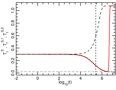
(b)

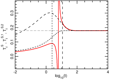
Figure 9: Fictive temperatures during the two stages of the Kovacs protocol: (a) aging at $T_{1}$, (b) time evolution at $T_{2}$ leading to the Kovacs hump. On panel (b) the vertical scale has been truncated to allow a better view of the behavior of the fictive temperatures relative to the eigenmodes. Red full line: $T_{f}^{S,\mathrm{transfo}}$ computed along the thermodynamic trajectory. Short-dash and long-dash black curves: $T_{f}^{S,1}$ and $T_{f}^{S,2}$, the fictive temperatures relative to the two eigenmodes. The vertical lines mark the relaxation times of the modes $\tau_{1}$ (short dash) and $\tau_{2}$ (long dash) at each thermostat temperature $T$ marked by the thin dashed horizontal line.

Figure 9 shows that the concept of fictive temperature is also useful to understand the time evolution of the system during the two stages of the Kovacs protocol. For the aging stage (Fig. 9-a) we notice that all fictive temperatures $T_{f}^{S,\mathrm{transfo}}$, $T_{f}^{S,1}$, $T_{f}^{S,2}$, start from the value $0.3$ which was the temperature of the equilibrium state before the system was quenched to $T_{1}$. They start evolving around $t=\tau_{1}(T_{1})$, which is the time necessary for the relaxation of the fastest mode to show up. In this time range the $P_{i}$ start to evolve, and, as a result, all fictive temperatures change. $T_{f}^{S,\mathrm{transfo}}$ closely follows the fictive temperature $T_{f}^{S,1}$ because, at this low temperature $T_{2}=0.02$, the two relaxation times are extremely different. As shown in Fig. 6, only mode 1 significantly evolves during the aging process. Therefore the path in the configuration space follows mode 1, so that $T_{f}^{S,\mathrm{transfo}}\approx T_{f}^{S,1}$. After mode 1 has equilibrated, its amplitude $a(t)$ has almost vanished and the evolution goes on along mode 2 only. Even though the variation of $b(t)$ is small, it is now the dominant mode in the system and therefore $T_{f}^{S,\mathrm{transfo}}\approx T_{f}^{S,2}$. The switch of $T_{f}^{S,\mathrm{transfo}}$ from $T_{f}^{S,1}$ to $T_{f}^{S,2}$ looks very sharp on Fig. 9-a but this is an artifact of the logarithmic scale used for time. Therefore the plot of the fictive temperatures allows a detailed analysis of the mechanisms behind the aging process. At the end of this stage, $T_{f}^{S,\mathrm{transfo}}$ is very different from the temperature of the thermostat, which tells us that the system is still strongly out of equilibrium in spite of this long aging period. Fig. 9-b allows a similar analysis for the process leading to the Kovacs hump, but, in this case the evolution is more complex. When the temperature is switched from $T_{1}$ to $T_{2}$, the eigenvectors of the modes change, and therefore the expressions of $T_{f}^{S,1}$, $T_{f}^{S,2}$ change too. The abrupt temperature rise from $T=0.02$ to $T=0.17856$ induces a change in the occupation of the three states (see Fig. 4-b). Initially $P_{3}$, was almost zero, giving very large ratios $P_{1}/P_{3}$ and $P_{2}/P_{3}$. As it raises significantly, the ratios decrease as well as the logarithms in the denominators of $T_{f}^{S,1}$, $T_{f}^{S,2}$. As a result both fictive temperatures tend to grow for the shorter times. $T_{f}^{S,1}$ smoothly approaches the system temperature $T_{2}$ while the initial growth of $T_{f}^{S,2}$ is large enough to bring it above $T_{2}$ and it finally reaches $T_{2}$ by decaying from above. For the Kovacs stage, the evolution of $T_{f}^{S,\mathrm{transfo}}$ is very peculiar, and this points out the complexity of the Kovacs relaxation. Initially, as mode 1 is the fastest, it dominates the evolution and therefore $T_{f}^{S,\mathrm{transfo}}$ evolves like $T_{f}^{S,1}$. In the last part of the process, as mode 1 has relaxed, $T_{f}^{S,\mathrm{transfo}}$ evolves like $T_{f}^{S,2}$ as in the aging period. But, in between, around the maximum of the Kovacs hump between $\tau_{1}(T_{2})$ and $\tau_{2}(T_{2})$, $T_{f}^{S,\mathrm{transfo}}$ shows an unexpected behavior, with a divergence and even a short time interval where it is negative. To understand it, one has to look at the definition of the fictive temperature given by Eq. (10) and at the behavior of the energy (Fig. 4) and of the entropy discussed below (Fig. 11). Both show a hump. At the maximum of the Kovacs hump we have $dE=0$, and it changes sign when the Kovacs hump occurs. Similarly the entropy shows a hump with $dS=0$, and a change of sign of $dS$ in the vicinity. But, due to the entropy production (Sec. V.2) the maximum of the entropy does not exactly coincide with the maximum of the energy. The vanishing of $dS$ when $dE\not=0$ causes the divergence seen on $T_{f}^{S,\mathrm{transfo}}$, and the changes of signs of $dE$ and $dS$ explain the surprising negative fictive temperature $T_{f}^{S,\mathrm{transfo}}$.

This analysis confirms that a unique fictive temperature cannot be defined for an out-of-equilibrium system which requires several configuration parameters besides its thermodynamic variables to be fully characterized. Nevertheless this concept can be defined for a specific transformation, and particularly for the eigenmodes. This gives a measurement of the distance to equilibrium regarding each relaxation time of the system. Following $T_{f}^{S,\mathrm{transfo}}$ and its relationship with the fictive temperatures associated to each mode gives a further understanding of the behavior of an out-of-equilibrium system.

Particular case of the two-state system

The same thermodynamic definition of the fictive temperature can also be applied to the two-state system of Fig. 1-b. Using $P_{1}+P_{2}=1$, and therefore $dP_{2}=-dP_{1}$, Eq. 11 reduces to

$$T_{f}^{S}=-\frac{E_{1}-E_{2}}{\ln\left(\frac{P_{1}}{P_{2}}\right)}\;.$$ (16)

For this system the fictive temperature does not depend on the particular transformation which is considered because $dP_{1}$ does not appear in its expression. This should not be a surprise because the state of this simple system is fully described by one variable, which could be either $P_{1}$ or the thermodynamic temperature, whether the system is in equilibrium or not. As we noticed, this two-state system does not show the Kovacs effect. In this case the temperature $T_{2}$ for which $E_{1}=E^{\mathrm{eq}}(T_{2})$ is the (unique) fictive temperature. It means that the state reached after the aging state, when the system is brought to $T_{2}$, is already its equilibrium state so that it does not evolve any more.

V.2 Entropy

The statistical entropy of a model based on a set of energy states $E_{i}$, occupied with probabilities $P_{i}$, over which the system evolves by transitions from a state to another is given by

$${S}=-\sum_{i}P_{i}\;\ln P_{i}$$ (17)

where we have set $k_{B}=1$ because we measure temperatures in energy units. For the three-state system it can be computed exactly in a numerical simulation and even calculated analytically for all transformations involving only constant-temperature processes and sharp temperature jumps. However, for a discussion of glassy properties, it would be useful to get an expression of the entropy which provides a deeper insight by distinguishing the equilibrium contribution from the part coming from out-of-equilibrium transformations. This can be done by exhibiting the equilibrium values within $P_{i}$ using

$$P_{i}(T,t)=P_{i}^{\mathrm{eq}}(T)+Q_{i}(T,t)\;,$$ (18)

as we did earlier. For any transformation which is not too far from equilibrium, i.e. such that $Q_{i}/P_{i}^{\mathrm{eq}}\ll 1$ then $\ln P_{i}$ can be expanded as

$$\ln P_{i} =\ln P_{i}^{\mathrm{eq}}+\ln\left(1+\frac{Q_{i}}{P_{i}^{\mathrm{eq}}}\right)$$

$$=\ln P_{i}^{\mathrm{eq}}+\frac{Q_{i}}{P_{i}^{\mathrm{eq}}}-\frac{1}{2}\left[\frac{Q_{i}}{P_{i}^{\mathrm{eq}}}\right]^{2}+O[(Q_{i}/P_{i}^{\mathrm{eq}})^{3}]\;.$$ (19)

Using Eq.(17), this leads to an approximate expression of the entropy as

$${S}= -\sum_{i}P_{i}^{\mathrm{eq}}\;\ln P_{i}^{\mathrm{eq}}$$

$$-\sum_{i}Q_{i}\ln P_{i}^{\mathrm{eq}}-\frac{1}{2}\sum_{i}P_{i}^{\mathrm{eq}}\left[\frac{Q_{i}}{P_{i}^{\mathrm{eq}}}\right]^{2}$$

$$+O[(Q_{i}/P_{i}^{\mathrm{eq}})^{3}]\;.$$ (20)

which can be written

$${S}={S^{\mathrm{eq}}}+\Delta S_{1}+\Delta S_{2}+O[(Q_{i}/P_{i}^{\mathrm{eq}})^{3}]\;.$$ (21)

where $S^{\mathrm{eq}}$ is the entropy at equilibrium at temperature $T$. Taking into account $\sum_{i}Q_{i}=0$ and introducing the values (2) of $P_{i}^{\mathrm{eq}}$, the correction to the entropy up to first order in $Q_{i}/P_{i}^{\mathrm{eq}}$ is simply

$${\Delta S_{1}}=-\sum_{i}Q_{i}\ln P_{i}^{\mathrm{eq}}=\frac{E-E^{\mathrm{eq}}}{T}\;.$$ (22)

The second order correction to the entropy is

$${\Delta S_{2}}=-\frac{1}{2}\left\langle\left[\frac{Q_{i}}{P_{i}^{\mathrm{eq}}}\right]^{2}\right\rangle\;.$$ (23)

where the bracket means the statistical averaging.

For the three-state system, the different expressions of the entropy can be computed analytically for any transformation at constant temperature, starting from a known state $(P_{1},P_{2})$, as shown in Sec. IV.

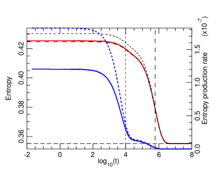
Figure 10: Left scale: entropy for the approach to equilibrium in an abrupt temperature change from $T=0.08$ to $T=0.07$. Red curve: Numerical result from Eq. (17) (which could also be obtained analytically as we can compute $P_{i}(t)$). Short-dash and long-dash black lines: first and second order expansions. Note that, in this case which does not include a big $T$-jump the second order expansion for the entropy is accurate.
Right scale: Entropy production rate for the same process. Blue full line: exact result from Eq. (28) and dashed blue line: approximate value from Eq. (27).
The vertical lines mark the relaxation times (full line $\tau_{1}$, long-dash line $\tau_{2}$).

Figure 10 shows the variation of the entropy when the three-state system approaches equilibrium at $T=0.07$ from an initial equilibrium at $T=0.08$, chosen sufficiently close to the final temperature to avoid large deviations of the probabilities from their equilibrium values to guarantee the validity of the expansion. The red curve shows the exact value of the entropy. The first order approximation

$${S}={S^{\mathrm{eq}}}+\Delta S_{1}\;.$$ (24)

(small-dash black curve) overestimates the entropy, but the second order expansion

$${S}={S^{\mathrm{eq}}}+\Delta S_{1}+\Delta S_{2}\;.$$ (25)

(long-dash black curve) is able to closely approach the actual entropy change in the process.

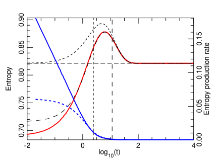
Figure 11: Left scale: entropy for the Kovacs time evolution. Red curve: Numerical result from Eq. (17) (which could also be obtained analytically as we can compute $P_{i}(t)$). Short-dash and long-dash black lines: first and second order expansions. In this case the calculation is less accurate than for the case shown in Fig. 10 because the condition $Q_{i}/P_{i}^{\mathrm{eq}}\ll 1$ is not satisfied in the first part of the time evolution.
Right scale: Entropy production rate for the same process. Blue full line: exact result from Eq. (28) and dashed blue line: approximate value from Eq. (27).
The vertical lines mark the relaxation times (full line $\tau_{1}$, long-dash line $\tau_{2}$).

Figure 11 shows the same entropy expansion for last stage of the Kovacs protocol, at constant temperature $T_{2}$, in which the energy exhibits the Kovacs hump plotted in Fig. 4. The exact calculation (red curve) shows that the entropy increases during the process. The first order expansion of Eq. (V.2) shows a hump in the entropy but no overall entropy change in the whole process, in agreement with Eq. (22), because at the end of the process the energy recovers the value that it had the beginning. The second order correction detects the entropy increase, however it does not give an accurate evaluation of the entropy in the early stage of the evolution. This is due to the large temperature jump, from $T_{=}0.02$ to $T_{2}=0.17856$ after which the condition $Q_{i}/P_{i}^{\mathrm{eq}}\ll 1$ is not satisfied.

Entropy production

The variation of the entropy in a transformation can be separated into two terms

$$\Delta S=\Delta_{e}S+\Delta_{i}S\;,$$ (26)

where $\Delta_{e}S=\Delta E/T$ is the contribution coming from the energy exchange with the outside and $\Delta_{i}S$ is the contribution coming from internal transformations in the system, called the entropy production, which is never negative $\Delta_{i}S\geq 0$ and vanishes for reversible processes. This concept, familiar for the thermodynamic entropy in out-of-equilibrium system GLANSDORFF , also extends to the statistical entropy in multilevel systems LANGER . For a transformation at constant temperature, $\Delta_{i}S$ is related to the variation of the thermodynamic function free energy $F=E-TS$ because $\Delta F/T=\Delta E/T-\Delta S$ so that $\Delta_{i}S=-\Delta F/T$.

The approximate expression of the entropy, derived above, can also be used to express the rate of entropy production $d_{i}S/dt$ for a transformation starting from an equilibrium state because Eq. (22) shows that $\Delta S_{1}=(E-E^{\mathrm{eq}})/T=\Delta_{e}S$ and therefore $\Delta_{i}S=\Delta S_{2}+O[(Q_{i}/P_{i}^{\mathrm{eq}})^{3}]$. Taking the time derivative of this equation, and using Eq. (23) gives

$${\frac{d_{i}S}{dt}}=-\frac{1}{T}\frac{dF}{dt}\approx-\sum_{i}\frac{Q_{i}}{P_{i}^{\mathrm{eq}}}\frac{dQ_{i}}{dt}>0\;,$$ (27)

up to second order in $Q_{i}/P_{i}^{\mathrm{eq}}$. This value, which can be computed analytically as shown in Sec. IV, can be compared with the exact value of ${d_{i}S}/{dt}$ deduced from the expression (17) of the entropy by subtracting $d_{e}S=-\sum\ln P_{i}^{\mathrm{eq}}\;dP_{i}$ which gives

$$\frac{d_{i}S}{dt}=-\sum_{i}\ln\left(\frac{P_{i}}{P_{i}^{\mathrm{eq}}}\right)\frac{dP_{i}}{dt}$$ (28)

For the three-state system, figures 10 and 11 show the exact and approximated expressions of the entropy creation rate as a function of time for the approach to equilibrium (Fig. 10) and the constant temperature evolution at temperature $T_{2}$ in the protocol to observe the Kovacs effect (Fig. 11). As expected, the entropy production rate is positive at the beginning of relaxation when the system is outside equilibrium. It then tends towards zero with different shapes for the two different relaxational processes until the system reaches equilibrium for longer time. The full-line blue curves (exact values from Eq. (28) ) or the dashed-lines blue curves (approximate expressions from Eq. (27) ) differ significantly at the earlier stages of each of the transformations. This is because, after the temperature jumps that started the processes, the second order expansion in $Q_{i}/P_{i}^{\mathrm{eq}}$ is not sufficient. This is obvious in the case of Fig. 11 because the plots of the entropy (red full line and black dashed lines on the same figure) show that even its second order expansion of the entropy is not good in the early stage of the transformation. This is less obvious for Fig. 10 because the plots of the entropy (red full line and black dashed lines) show that the approximation of the entropy up to the second order in $Q_{i}/P_{i}^{\mathrm{eq}}$ is not bad. However the entropy production is small, and results from a difference between two nearly equal terms $\Delta S$ and $\Delta_{e}S$, so that even a small error in the calculation of $\Delta_{e}S$ can have a very significant effect. Since the entropy production term is always a term of second order in the departure from equilibrium, it is generally small. Accurately fulfilling the criterion $Q_{i}/P_{i}^{\mathrm{eq}}\ll 1$ is of great importance for such a small contribution. It is less critical for contributions of first order such as the entropy. In calculations, as well as in experiments JABRAOUI , determining the entropy production is challenging.

For the protocol to observe the Kovacs effect, as expected the Kovacs hump in energy shows up in the entropy change through $\Delta_{e}S$, but the red curve for the entropy computed by ${S}=-\sum P_{i}\;\ln P_{i}$ shows a large additional contribution which results in a significant rise of the entropy. This is due to the irreversibility of the process. The blue curve shows that the (positive) entropy production rate is particularly strong at the beginning of the time evolution, which is the source of the large entropy rise. Then the system evolves towards equilibrium and the entropy production rate drops. When time has reached $\tau_{2}(T_{2})$, the entropy production has almost disappeared, as expected in equilibrium, and the entropy change is almost determined by the contribution coming from the energy exchange.

VI Discussion

The Kovacs effect is a nice example of out-of-equilibrium process because it clearly shows that the state of such a system cannot be described only by its thermodynamic equilibrium variables. This effect is usually considered as typical of glasses which have a continuum of relaxation times but it is actually more generic. It can be observed in a system as simple as the three-state system, with only two relaxation times. However it does not exist for the even simpler two-state system. This two-state system can show some glass-like properties, such as a negative heat capacity BISQUERT , however it lacks a fundamental property because, when its energy is specified, its configuration, described by the unique variable $P_{1}$ is also fully determined. In the three-state system this one-to-one correspondence between the energy and the configuration of the system is broken. A given energy can be realized by various $P_{1}$, $P_{2}$ configurations.

The three-state system is an interesting model to study out-of-equilibrium properties because it is probably the simplest system which has the necessary ingredients. It is too simple to describe the glass transition by itself, but it nevertheless exhibits fundamental properties of glasses, such as the Kovacs effect. And moreover it allows an analytical description which leads to a basic understanding of the phenomena. For instance the time at which the Kovacs hump is observed can be clearly linked to the relaxation times of the system. This provides some answer to a question raised by Bertin et al. in ref. BERTIN : how to extract microscopic information on a system from the Kovacs hump? Our results show that its shape contains direct information on the statistics of the relaxation times in the system.

One may wonder whether the three-state model can be relevant to describe some properties of complex non-equilibrium systems. An interesting example is provided by spin models of strong and fragile glasses studied in Ref. ARENZON . This paper points out that the Kovacs effect seems to provide an alternative independent method to obtain the equilibration time of the system because the time at which the peak occurs varies like this equilibration time. This is exactly what the three-state model gives by showing that the Kovacs hump rises after the shortest relaxation time of the system and drops after the longest relaxation time. The paper ARENZON makes a closer connection to the ideas behind the three-state model because it studies how a complex spin systems explores its inherent structures, i.e. the basins of attraction of the energy minima. It shows that the distribution of the inherent structures explored far from equilibrium differs in depth from the distribution explored in equilibrium. A similar analysis was made in a study of the Kovacs effect in a molecular liquid MOSSA . It found that, when the system ages it explores regions of the potential energy landscape which are no explored at equilibrium. The three-state model shows the same phenomena when a fast quenching brings it very far from equilibrium, as shown in Fig. 12 for an example of the Kovacs effect in which the aging started from $T=0.50$ instead of $T=0.30$ as in the cases discussed earlier. The largest temperature jump brought the system farther from equilibrium when the temperature evolution at constant temperature ($T=0.2110$) started. The plot of the energy versus time on Fig. 12 shows the usual hump, but the variation of the occupation probabilities $P_{1}$, $P_{2}$, $P_{3}$ versus time shows a peculiar evolution because two curves cross each other. At the end of aging $P_{1}$ (for $E_{1}=-0.40$) was lower than $P_{2}$ (for $E_{2}=-0.25$). In equilibrium we don’t expect that an energy level is more populated than another one which has a lower energy, but this can be observed if the system is far from equilibrium. As observed in complex systems, the three-state model explores such states.

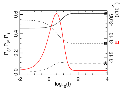
Figure 12: Energy (red curve, right scale) and probabilities $P_{1}$,$P_{2}$, $P_{3}$ (black curves, left scale) versus time (in log scale) during the time evolution at constant temperature $T_{2}=0.2110$ after aging for $1.8\,10^{7}\,$t.u. at temperature $T_{1}=0.02$ in the study of the Kovacs effects. The conditions are very similar to the case shown in Fig. 4 except that the aging started from an equilibrium temperature $T^{\mathrm{ini}}=0.50$ instead of $0.30$ so that the cooling rate was faster. Full black line $P_{1}$, short-dash black line $P_{2}$, long-dash black line $P_{3}$. The points at the right side of the graph show the values of the equilibrium probabilities at $T_{2}$ : circle $P_{1}^{\mathrm{eq}}$, square $P_{2}^{\mathrm{eq}}$, star $P_{3}^{\mathrm{eq}}$.

It seems that a model as simple as the three-state model cannot quantitatively describe the properties of actual glassy samples but it might actually be closer to experimental systems than one could think. In many glassy systems, such as polymers, instead of a continuum spectrum of relaxation times, there are groups of “slow modes” for instance associated to molecular reorientations, which are well separated from “fast modes”. In Ref PEREZ-EULATE , long aging experiments on polymers at temperatures lower than the glass transition temperature show that, at such low temperatures, it is possible to reach a plateau in enthalpy (by a fast relaxation mechanism) without disturbing the classical alpha relaxation processes. It results in an aging-time-dependent overshoot of the specific heat during heating, below the classical specific heat peak at the glass-transition temperature. The three-level system, with a relaxation of the fast mode at low temperature while the slow one is practically not disturbed (see Fig. 6), could be appropriate to explain this behavior. In this case two fictive temperatures such as those associated to each independent modes of the three level system should be involved. There are several experimental results which point to the interest of this simple model to analyze Kovacs-hump data on glasses. A recent example is provided by an article showing that the Kovacs hump is not only observed in the enthalpy of a glass but can also be detected in the amplitude of the Boson peak which corresponds to an enhanced low frequency (terahertz region) density of states as compared with the Debye square frequency law LUO-P . This may be related to our Fig. 9-b which shows a peak in the fictive temperature of the slow mode $T_{f}^{S,2}$, occurring near the time at which the Kovacs hump occurs, while $T_{f}^{S,1}$ for the fast mode increases monotonically. The paper suggests that a possible explanation of the experimental results could rely on a two-relaxation-time model already used earlier to propose a phenomenological analysis of Kovacs-hump-like non-monotonic relaxations of the Curie temperature in a metallic glass GREER and refractive index of $B_{2}O_{3}$. In these studies the frequencies of the two modes were simply fitted. It is tempting to try to go further with the three-state model which allows the computation of the shape of the Kovacs hump in addition to the determination of the relaxation times.

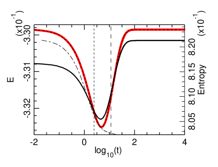
Figure 13: Reverse-Kovacs effect observed with the three-state model with $T^{\prime}_{0}=0.02$, $T^{\prime}_{1}=0.22$ and $T^{\prime}_{2}=0.17852$. The red curve (numerical result) superimposed on the short-dash black line (theoretical calculation) shows the variation of the energy (left scale) versus time (in log scale) during the time evolution at temperature $T^{\prime}_{2}$ after annealing for 10.12 t.u. at temperature $T^{\prime}_{1}$. The full black line shows the time evolution of the entropy (right scale) and the thin dash-dot line shows the variation of the entropy production (its scale, not shown on the graph, varies from 0 to $3.0\,10^{-3})$

In their experimental study of $B_{2}O_{3}$, Boesch et al. exhibited another memory effect which is a kind of “reverse-Kovacs effect”, later observed in other non-equilibrium systems TRIZAC ; KURSTEN . The protocol is to start from an equilibrium state at low temperature $T^{\prime}_{0}$, and then to anneal the sample at a higher temperature $T^{\prime}_{1}$ for a time so short that it cannot reach equilibrium. The annealing is interrupted when the refractive index reaches a prescribed value which is its value at equilibrium at a temperature $T^{\prime}_{2}<T^{\prime}_{1}$. Then the temperature is abruptly shifted to $T^{\prime}_{2}$ and the behavior of the refractive index is measured. As for the Kovacs effect, although the index already has its expected value in equilibrium at $T^{\prime}_{2}$, it does not stay constant but exhibits a non-monotonic evolution with the opposite sign of its evolution in the Kovacs effect, until it finally recovers its equilibrium value at temperature $T^{\prime}_{2}$. As shown in Fig. 13, this peculiar memory effect can also be observed with the three-state model with a similar protocol. We selected $T^{\prime}_{0}=0.02$, $T^{\prime}_{1}=0.22$ and an annealing time of $10.12\;$t.u. at $T^{\prime}_{1}$ so that the energy reaches the equilibrium value $E^{\mathrm{eq}}(T^{\prime}_{2}=0.17852)$, a temperature very close to the temperature $T_{2}=0.17856$ at which we had studied the Kovacs effect plotted on Fig. 4. The time evolution of the energy at $T^{\prime}_{2}$ shows a dip instead of the Kovacs hump. As we have chosen a value $T^{\prime}_{2}$ very close to the temperature $T_{2}$ at which we studied the Kovacs effect shown in Fig. 4, the relaxation times are almost the same in the two cases and the shape of the dip looks as a mirror image of the Kovacs hump. However its magnitude is smaller than the magnitude of the hump because the annealing at $T^{\prime}_{1}=0.22$ brought the system closer to equilibrium than the annealing at $T_{1}=0.02$ used to get the Kovacs effect. In this reverse-Kovacs effect, because the energy drops in the dip, the entropy shows a minimum (see Fig. 13), but, as expected for this irreversible process the entropy production is always positive and the entropy during the evolution at $T^{\prime}_{2}$ increases. Together with the asymmetric approach to equilibrium discussed earlier, this example shows the ability of the three-state model to describe a large variety of phenomena experimentally observed in glasses.

It is interesting to examine whether the three-state system contains the ingredients required by Bouchbinder and Langer to model the Kovacs effect BOUCHBINDER . Their basic assumption is that a glass consists of two interacting subsystems which have very different characteristic times and can fall out of thermal equilibrium with each other. The two eigenmodes of the three-state system play this role. Figure 6, plotting the amplitude of these modes at the end of the aging period in the Kovacs protocol shows that one mode has already relaxed to equilibrium while the second has not. Thus the two modes can indeed fall out of thermal equilibrium with each other. We have shown that we can affect a fictive temperature to each mode, and there are states in which the two fictive temperatures are different. The third, and less obvious condition that there exists a mechanism in which the fast subsystem can produce changes in the effective temperature of the slow subsystem seems to be absent in the three-state model because the eigenmodes are independent from each other. However because the dynamics of the model is driven by the thermal bath which is responsible for the evolution of the state populations, this is enough to ensure that the slow subsystem keeps evolving even when the fast mode is equilibrated, although it cannot be attributed to a weak coupling between the two eigenmodes. In spite of the similarities between the three-state model and the ideas of Bouchbinder and Langer, the concepts behind the models are different. For the three-state model, the states are inspired by inherent structures NAKAGAWA . Consequently they can be viewed as describing configurational states. The kinetic fast degrees of freedom are absent from the model and instead replaced by the thermostat that controls the transition between the configurational states.

As the three-state model belongs to a class of systems described by a master equation studied in Ref. PradosJSTAT one can ask whether our results could be deduced from the general results derived in this work, and applied to complex spin systems in RUIZ-GARCIA . However, in the general case studied in Ref. PradosJSTAT the analysis of the Kovacs effect can only be made in a linear approximation. This is interesting in theoretical models because general properties of the Kovacs hump can be obtained, but it is a severe restriction to analyze experimental data on glasses. In the study of the Ising model of Ref RUIZ-GARCIA the linear response results are considered as fine up to temperature jumps such that the relative change of the relaxation time between the initial and final temperatures is about ten percent. In glass transitions relaxation times often change by many orders of magnitudes. In the results presented in Fig. 4, the relaxation times during aging at $T=0.02$ are $\tau_{1}=0.2681\,10^{6}$ and $\tau_{2}=0.8708\,10^{12}$ while their values drop to $\tau_{1}=2.471$ and $\tau_{2}=11.59$ after the temperature jump to $T=0.17856$ which shows the Kovacs hump. The change is so large that only exact results, which can be obtained for the three-state model, can quantitatively describe the Kovacs hump in this case.

In spite of its simplicity, this model has limitations in the analytical analysis that it allows. The calculations are simple for all processes occurring at constant temperature, including out-of-equilibrium processes triggered by a sharp temperature jump. But for processes involving a continuous driving of the temperature, the analytical calculations become unpractical because they require an expansion on a basis which is continuously evolving.

While a thermodynamic definition of the fictive temperature is possible for a two-level system, it is meaningless for a three-level system. However, it is possible to define two particular fictive temperatures, each one being associated to an eigenmode of the system. This suggests a generalization of the idea of fictive temperature in the case of a real glass. As shown in Fig. 9, each fictive temperatures $T_{f}^{S,1}$, $T_{f}^{S,2}$ determines the variation of the fictive temperature $T_{f}^{S,\mathrm{transfo}}$ of the system along its trajectory in the configuration space for a time range around the corresponding relaxation times $\tau_{1}$ and $\tau_{2}$. This suggests that a complex system, with many relaxation times should be characterized by a distribution of fictive temperatures. The full distribution is certainly hard to determine, but beyond the mean which might correspond to the usual concept of fictive temperature, further moments of this distribution could provide a complementary description of the thermodynamic state of a complex out-of-equilibrium system.

All this approach could be generalized to $N$-level systems, for which $N-1$ independent internal variables are sufficient to follow the non-equilibrium nature of complex systems. However, moving from $N=2$ to $N=3$ is the essential step to get a rich behavior because it is sufficient to generate a system which is not fully determined by its thermodynamic variables only. The three-state system is the simplest of complex systems!

Appendix A Analytical solution for the time dependence of the occupation probabilities

In terms of the deviations $Q_{i}$ with respect to equilibrium probabilities, the two coupled equations for $P_{1}$ and $P_{2}$ become an equation for the vector $\vec{Q}$, having the components $Q_{1}$ and $Q_{2}$ which can be written as

$$\frac{d}{dt}\left(\begin{array}[]{c}Q_{1}\\ Q_{2}\end{array}\right)=\left(\begin{array}[]{cc}-A&B\\ B^{\prime}&-A^{\prime}\\ \end{array}\right)\left(\begin{array}[]{c}Q_{1}\\ Q_{2}\end{array}\right)=M\left(\begin{array}[]{c}Q_{1}\\ Q_{2}\end{array}\right)$$ (37)

with

$$A=e^{-B_{12}/T}+e^{-B_{13}/T}+e^{-B_{31}/T}$$

$$B=e^{-B_{21}/T}-e^{-B_{31}/T}$$

$$A^{\prime}=e^{-B_{21}/T}+e^{-B_{23}/T}+e^{-B_{32}/T}$$

$$B^{\prime}=e^{-B_{12}/T}-e^{-B_{32}/T}$$

To solve equation (37) we can expand $\vec{Q}$ on the eigenvectors $\vec{U}^{(1)}$ and $\vec{U}^{(2)}$ which diagonalize the matrix $M$

$$M\vec{U}^{(i)}=\lambda_{i}\vec{U}^{(i)}\;.$$ (39)

The eigenvalues $\lambda_{1}$ and $\lambda_{2}$ are

$$\lambda_{1,2}=\frac{1}{2}\left[-(A+A^{\prime})\pm\sqrt{\Delta}\right]$$ (40)

with $\Delta=(A-A^{\prime})^{2}+4BB^{\prime}$. The system parameters which are compatible with the existence of a thermal equilibrium are such that $\lambda_{1,2}<0$. Each eigenvalue corresponds to an eigenvector $\vec{U}^{(i)}$ ($i=1,2$). Its components are denoted as

$$\vec{U}^{(i)}=\left(\begin{array}[]{c}U_{1}^{(i)}\\ U_{2}^{(i)}\end{array}\right)$$ (43)

Matrix $M$ is not a symmetric matrix. It is not orthogonal and it is easy to check that its eigenvectors are not orthogonal to each other, i.e.

$$U_{1}^{(1)}\;U_{1}^{(2)}+U_{2}^{(1)}\;U_{2}^{(2)}\not=0\;.$$ (44)

However those vector are not colinear

$$U_{1}^{(1)}\;U_{2}^{(2)}-U_{2}^{(1)}\;U_{1}^{(2)}\not=0$$ (45)

and therefore they nevertheless define a basis for the $Q_{1}$, $Q_{2}$ space. On this basis $\vec{Q}$ can be written as

$$\vec{Q}=a(t)\vec{U}^{(1)}+b(t)\vec{U}^{(2)}\;.$$ (46)

This calculation holds for any value of the temperature, which could be time-dependent, as for instance when the system is slowly cooled at a given rate. However, in practice, the calculation is only useful for all situations in which the temperature is kept fixed because then the matrix $M$ is time-independent and so are its eigenvectors. In the following we assume that the temperature is either a constant or that it evolves by abrupt jumps so that the temperature protocol can be decomposed in segments during which the temperature stays constant, as for instance in the protocol used to observe the Kovacs effect.

Equation (46) defines a system of two scalar equations for $a$ and $b$. Its determinant is

$$D=\left|\begin{array}[]{cc}U_{1}^{(1)}&U_{1}^{(2)}\\ U_{2}^{(1)}&U_{2}^{(2)}\end{array}\right|\;.$$ (49)

It does not vanish due to the relation (45) so that, if $Q_{1}(t)$, $Q_{2}(t)$ are known, for instance from numerical integration results, the contributions $a(t)$, $b(t)$ of the two eigenmodes can be determined.

However it is more interesting to get $a(t)$, $b(t)$ by analytically solving Eq. (37), which leads to

$$\frac{da(t)}{dt}\vec{U}^{(1)}+\frac{db(t)}{dt}\vec{U}^{(2)}=\lambda_{1}a(t)\vec{U}^{(1)}+\lambda_{2}b(t)\vec{U}^{(2)}\;$$ (50)

which can be viewed as a system of two equations for the unknowns

$$X=\frac{da(t)}{dt}-\lambda_{1}a(t)\qquad Y=\frac{db(t)}{dt}-\lambda_{2}b(t)\;,$$ (51)

which can be written

$$U_{1}^{(1)}X+U_{1}^{(2)}Y =0$$

$$U_{2}^{(1)}X+U_{2}^{(2)}Y =0\;.$$ (52)

The determinant of this system is again the determinant $D$ of Eq. (49), which is non-zero. As the right-hand-side of the system is zero, the only solution of the system is $X=0$, $Y=0$. According to (51) it implies that the general solutions for $a(t)$ and $b(t)$ are exponential relaxations

$$a(t) =a(t=0)\exp[-t/\tau_{1}]$$

$$b(t) =b(t=0)\exp[-t/\tau_{2}]$$ (53)

where $\tau_{1,2}=-1/\lambda_{1,2}$.

References

- (1) A.J. Kovacs, Transition vitreuse dans les polymères amorphes. Etude phénoménologique. Fortsch. Hochpoly.-Forsch., 3 394-507 (1963)
- (2) L. Berthier and G. Biroli, Theoretical perspective on the glass transition and amorphous materials. Rev. Mod. Phys. 83, 587-645 (2011)
- (3) S.B. Thomas and G.S. Park, Studies on glass: IV. Some Specific Heat Data on Boron Trioxide J. Phys. Chem. 35, 2091-2102 (1931)
- (4) L. Berthier and P. C. W. Holdsworth, Surfing on a critical line: Rejuvenation without chaos, memory without a hierarchical phase space EPL 58, 35 (2002)
- (5) E M Bertin, J-P Bouchaud, J-M Drouffe and C Godrèche, The Kovacs effect in model glasses J. Phys. A: Math. Gen. 36 (2003) 10701–10719
- (6) Gerardo Aquino, Luca Leuzzi, and Theo M. Nieuwenhuizen, Kovacs effect in a model for a fragile glass Phys. Rev. B 73, 094205-1-8 (2006)
- (7) S. Mossa and F. Sciortino Crossover (or Kovacs) Effect in an Aging Molecular Liquid Phys. Rev. Lett. 92, 045504-1-4 (2004)
- (8) E. Bouchbinder and J.S. Langer, Nonequilibrium thermodynamics of the Kovacs effect Soft Matter, 6, 3065–3073 (2010)
- (9) R.O. Davies and G.O. Jones, Thermodynamic and kinetic properties of glasses. Adv. Phys. 2, 370-410 (1953)
- (10) L. Leuzzi, A stroll among effective temperatures in aging systems: Limits and perspectives Journal of Non-Crystalline Solids 355, 686–693 (2009)
- (11) N. Nakagawa and M. Peyrard, The inherent structure landscape of a protein. PNAS 103, 5279-5284 (2006)
- (12) A. Prados and J.J. Brey, The Kovacs effect: a master equation analysis J. Stat. Mech, P02009 (2010)
- (13) A.Q. Tool, and C.G. Eichlin, Variations caused in the heating curves of glass by heat treatment. J. Am. Chem. Soc. 14 276-308 (1931)
- (14) L. Wondraczek, S. Sen, H. Behrens, and R.E. Youngman Structure-energy map of alkali borosilicate glasses: Effects of pressure and temperature Phys. Rev. B 76, 014202-1-8 (2007)
- (15) Xiaoju Guo, M. Potuzak, J.C. Mauro, D.C. Allan, T.J. Kiczenski, Yuanzheng Yue Unified approach for determining the enthalpic fictive temperature of glasses with arbitrary thermal history J. Non Crys. Solids 357, 3230-3236 (2011)
- (16) B. Carnahan, H.A. Luther, J.O. Wilkes, Applied Numerical Methods, John Wiley & Sons (1969)
- (17) M.A. DeBolt, A.J. Easteal, P.B. Macedo and C.T. Moynihan, Analysis of Structural Relaxation in Glass Using Rate Heating Data J. Am. Ceram. Soc. 59, 16-21 (1976)
- (18) J. Bisquert, Master equation approach to the non-equilibrium negative specific heat at the glass transition Am. J. Phys. 73 735-741 (2005)
- (19) H. Jabraoui, S. Ouaskit, J. Richard, J.-L. Garden Determination of the entropy production during glass transition: Theory and experiment. J. Non Crystalline Solids 553, 119907-1-13 (2020)
- (20) G. Aquino, A. Allahverdyan, and T.M. Nieuwenhuizen, Memory Effects in the Two-Level Model for Glasses PRL 101, 015901-1-4 (2008)
- (21) J. Valle-Orero, J.-L. Garden, A. Wildes; J. Richard, and M. Peyrard, Glassy behavior of denatured DNA films studied by Differential Scanning Calorimetry J. Phys. Chem. B 116, 4394-4042 (2012)
- (22) H.N. Ritland, Limitations of the Fictive Temperature Concept. J. Am. Ceramic Society 39 403-406 (1956)
- (23) M. Lulli, Chun-Shing Lee, Hai-Yao Deng, Cho-Tung Yip and Chi-Hang Lam Spatial Heterogeneities in Structural Temperature Cause Kovacs’ Expansion Gap Paradox in Aging of Glasses PRL 124, 095501 (2020)
- (24) P. Glansdorff and I. Prigogine, Thermodynamic Theory of Structure, Stability and Fluctuations Wiley-Interscience, New York, 1971
- (25) S.A. Langer, J.P. Sethna and E.R. Grannan, Nonequilibrium entropy and entropy distribution. Phys. Rev. B 41 2261-2278 (1990)
- (26) J.J. Arenzon and M. Sellitto Kovacs effect in facilitated spin models of strong and fragile glasses Eur. Phys. J. B 42, 543–548 (2004)
- (27) N. G. Perez-De Eulate and D. Cangialosi, The very long-term physical aging of glassy polymers Phys. Chem. Chem. Phys. 20, 12356-12361 (2018)
- (28) P. Luo, Y.Z. Li, H.Y. Bai, P. Wen, and W.H. Wang, Memory Effect Manifested by a Boson Peak in Metallic Glass Phys. Rev. Lett. 116, 175901 (2016)
- (29) A.L. Greer and J.A. Leake, Structural relaxation and crossover effect in a metallic glass J. Non-Cryst. Solids 33 291-297 (1979)
- (30) L. Boesch, A. Napolitano, P.B. Macedo, Spectrum of Volume Relaxation Times in J. Am. Ceram. Soc. 53, 148-153 (1970)
- (31) E. Trizac and A. Prados, Memory effect in uniformly heated granular gases Phys. Rev. E 90, 012204 (2014)
- (32) R. Kürsten, V. Sushkov and T. Ihle, Giant Kovacs-Like Memory Effect for Active Particles PRL 119, 188001 (2017)
- (33) M. Ruiz-Garcıía and A. Prados, Kovacs effect in the one-dimensional Ising model: A linear response analysis Phys. Rev. E 89, 012140 (2014)