Quasinormal spectra of scale-dependent Schwarzschild-de Sitter black holes

Abstract

We compute the quasinormal spectra for scalar, Dirac and electromagnetic perturbations of the Schwarzschild-de Sitter geometry in the framework of scale-dependent gravity, which is one of the current approaches to quantum gravity. Adopting the widely used WKB semi-classical approximation, we investigate the impact on the spectrum of the angular degree, the overtone number as well as the scale-dependent parameter for fixed black hole mass and cosmological constant. We summarize our numerical results in tables, and for better visualization, we show them graphically as well. All modes are found to be stable. Our findings show that both the real part and the absolute value of the imaginary part of the frequencies increase with the parameter $\epsilon$ that measures the deviation from the classical geometry. Therefore, in the framework of scale-dependent gravity the modes oscillate and decay faster in comparison with their classical counterparts.

I Introduction

Many astonishing predictions of Einstein’s general relativity GR (GR) have been confirmed over the last 100 years or so, since its formulation until today. On the one hand, the classical tests and solar system tests tests1 ; tests2 ; tests3 , and on the other hand, more recently, the first image of a black hole L1 ; L2 ; L3 ; L4 ; L5 ; L6 combined with the direct detections of gravitational waves ligo1 ; ligo2 ; ligo3 ; ligo4 ; ligo5 , from mergers of black hole (BH) and neutron star binary systems, have shown in the most convincing way that GR is a remarkable theory of gravity, and also they have provided us with the strongest evidence so far that black holes do exist in Nature and that they merge. Astrophysical BHs are supposed to be formed during the final stages of massive stars, primordial BHs may be formed in the early Universe from density inhomogeneities, and mini-black holes may be formed at colliders or in the atmosphere of the earth in TeV-scale gravity scenarios in D-brane constructions of the Standard Model miniBH1 ; miniBH2 ; miniBH3 .

As successful as it may be as a classical theory, at quantum level technically speaking GR falls into the class of non-renormalizable theories. Although by now we know how to extract quantum predictions from a non-renormalizable theory using the techniques of effective field theory (to which GR fits perfectly) Donoghue:1994dn , the problem remains. As of today, the quest for a consistent quantum theory of gravity is still an open task in modern theoretical physics. In the context of theories beyond classical GR, one may mention at least two approaches, namely either scale-dependent gravity Contreras:2013hua ; Koch:2015nva ; SD1 ; Rincon:2017ayr ; Hernandez-Arboleda:2018qdo ; Contreras:2018gct ; Canales:2018tbn ; Rincon:2019zxk ; Rincon:2018lyd ; Contreras:2019fwu ; Fathi:2019jid ; PRL2 ; Contreras:2018swc ; Sendra:2018vux ; SD2 ; SD3 ; SD4 ; SD5 ; SD6 ; SD7 ; ourprd or improvement asymptotically safe gravity Bonanno:2000ep ; Bonanno:2001xi ; Reuter:2003ca ; Koch:2014cqa ; Gonzalez:2015upa . In both approaches the basic quantities that enter into the action defining the model at hand, such as Newton’s constant, cosmological constant etc, become scale dependent quantities. This does not come as a surprise of course, since scale dependence at the level of the effective action is a generic feature of ordinary quantum field theory.

Realistic black holes in Nature are in a constant interaction with their environment. When a black hole is perturbed, it responds by emitting gravitational waves. Quasinormal modes (QNMs) are characteristic frequencies with a non-vanishing imaginary part, which encode the information on how black holes relax after the perturbation has been applied. The QN frequencies depend on the details of the geometry and on the type of the perturbation (scalar, vector, tensor or fermionic), but not on the initial conditions. Black hole perturbation theory wheeler ; zerilli1 ; zerilli2 ; zerilli3 ; moncrief ; teukolsky and QNMs become relevant during the ring down phase of a black hole merger, the stage where a single distorted object is formed, and where the geometry of space-time undergoes dumped oscillations due to the emission of gravitational waves. Thanks to gravitational wave Astronomy we have now a powerful tool at our disposal to test gravitation under extreme conditions. For excellent reviews on the topic see review1 ; review2 ; review3 , and also the Chandrasekhar’s monograph chandra , which is the standard textbook on the mathematical aspects of black holes.

The current cosmic acceleration Riess:1998cb ; Perlmutter:1998np motivates the study of space-times with a positive cosmological constant. The maximally symmetric space-time of Einstein’s field equations with a positive cosmological constant without the presence of matter fields is the Schwarzschild-de Sitter geometry, characterized by the cosmological constant itself and the mass of the black hole. The quasinormal frequencies of the Schwarzschild-de Sitter in four dimensions and higher dimensions have been studied e.g. in lemos ; molina ; Zhidenko:2003wq ; Konoplya:2004uk ; LopezOrtega:2006my ; Kodama:2003jz ; panotop1 and references therein. Given the importance and relevance of the QNMs of black holes in gravitational wave Astronomy, it would be interesting to see what kind of spectra are expected from scale-dependent black holes.

In black hole physics the impact of the SD scenario on properties of black holes has been studied over the last years, and it has been found that the scale dependence modifies the horizon, the thermodynamics as well as the quasinormal spectra of classical black hole backgrounds SD1 ; SD2 ; SD3 ; SD4 ; SD5 ; SD6 ; SD7 ; ourprd . However, to the best of our knowledge, the QN modes of the four-dimensional scale-dependent Schwarzschild-de Sitter geometry have not been studied yet. Therefore, in the present work we propose to compute the QN spectra for scalar, Dirac, and electromagnetic perturbations of the SD Schwarzschild-de Sitter in four dimensions, filling thus a gap in the literature, and also making a direct comparison with the frequencies of the classical Schwarzschild-de Sitter solution.

The plan of our work is the following: In the next section we present the wave equations with the corresponding effective potential barrier for scalar, Dirac and electromagnetic perturbations, while in section three we briefly review the effective field equations in the framework of scale-dependent gravity. In section four we compute the quasinormal frequencies adopting the WKB approximation of 6th order, and we discuss our results. Finally, we summarize our work with some concluding remarks in section five. We adopt the mostly positive metric signature $(-,+,+,+)$, and we work in geometrical units where the universal constants are set to unity, $c=1=G_{0}$.

II Wave equations for massless scalar, Dirac and electromagnetic perturbations

In this section we present the wave equation and the corresponding effective potential barrier for massless scalar, Dirac and electromagnetic perturbations. We consider a fixed gravitational background (static, spherically symmetric) in Schwarzschild-like coordinates $t,r,\theta,\phi$ of the form

$$ds^{2}=-f(r)dt^{2}+f(r)^{-1}dr^{2}+r^{2}(d\theta^{2}+\sin^{2}(\theta)d\phi^{2})$$ (1)

with a given lapse function $f(r)$. Then we perturb that geometry by throwing in a probe field, and we study its propagation.

II.1 Spin zero case (scalar field)

The wave equation of a massless minimally coupled scalar field $\Phi$ is given by the usual Klein-Gordon equation, namely coupling ; p11 ; p12

$$\frac{1}{\sqrt{-g}}\partial_{\mu}\Bigl{(}\sqrt{-g}g^{\mu\nu}\partial_{\nu}\Bigl{)}\Phi=0$$ (2)

In order to solve the previous equation, we apply the separation of variables making the usual ansatz:

$$\Phi(t,r,\theta,\phi)=e^{-i\omega t}\frac{\psi(r)}{r}Y_{l}^{m}(\theta,\phi)$$ (3)

where $Y_{l}^{m}$ are the usual spherical harmonics, and $\omega$ is the frequency to be determined. Making the previous ansatz it is straightforward to obtain for the radial part a Schrödinger-like equation

$$\frac{\mathrm{d}^{2}\psi}{\mathrm{d}x^{2}}+[\omega^{2}-V(x)]\psi=0$$ (4)

with $x$ being the tortoise coordinate, i.e.,

$$x\equiv\int\frac{\mathrm{d}r}{f(r)}$$ (5)

Finally, the effective potential barrier is given by

$$V_{s}(r)=f(r)\>\left(\frac{l(l+1)}{r^{2}}+\frac{f^{\prime}(r)}{r}\right),\;\;\;\;l\geq 0$$ (6)

where the prime denotes differentiation with respect to $r$, and $l$ is the angular degree.

II.2 Spin one-half case (Dirac field)

Fermions are coupled to gravity in the vierbein formalism. Let us here briefly review the formalism, and present the wave equation with the corresponding potential following Destounis:2018qnb . First we introduce the tetrad or vierbein, $e_{a}^{\mu}$, defined by

$$e_{\mu}^{a}e_{\nu}^{b}\eta_{ab}=g_{\mu\nu}$$ (7)

with $\eta_{ab}$ being the flat Minkowski metric tensor. The vierbein carries two kinds of indices, namely a flat index $a$ as well a space-time index $\mu$, and it may be viewed as the ”square root” of the metric tensor $g_{\mu\nu}$. Next we define curved Dirac matrices as follows

$$G^{\mu}\equiv e_{a}^{\mu}\gamma^{a}$$ (8)

with the following property

$$\{\gamma^{a},\gamma^{b}\} = -2\eta^{ab}$$ (9)

$$\{G^{\mu},G^{\nu}\} = -2g^{ab}$$ (10)

where $\gamma^{a}$ are the usual Dirac matrices from the usual relativistic quantum mechanics in flat space-time. Finally, introducing the spin connection $\omega_{ab\mu},\Gamma_{\mu}$

$$\Gamma_{\mu} = -\frac{1}{8}\omega_{ab\mu}[\gamma^{a},\gamma^{b}]$$ (11)

$$\omega_{ab\mu} = \eta_{ac}[e_{\nu}^{c}e_{b}^{\lambda}\Gamma^{\nu}_{\mu\lambda}-e_{b}^{\lambda}\partial_{\mu}e_{\lambda}^{c}]$$ (12)

where $\Gamma^{\nu}_{\mu\lambda}$ are the Christoffel symbols, the Dirac equation for a spin one-half fermion $\Psi$ in curved space-time is given by

$$(iG^{\mu}D_{\mu}-m_{f})\Psi=0$$ (13)

where $m_{f}$ is the mass of the fermion, while the covariant derivative is defined to be $D_{\mu}\equiv\partial_{\mu}+\Gamma_{\mu}$.

For Dirac fermions we separate variables as before, where now we use the spinor spherical harmonics Finster:1998ak , and two radial parts

$$r^{-1}\>f(r)^{-1/4}\>F(r)$$ (14)

$$r^{-1}\>f(r)^{-1/4}\>iG(r)$$ (15)

for the upper and lower components of the Dirac spinor $\Psi$, respectively. In the massless limit, $m_{f}=0$, one obtains the following equations Destounis:2018qnb

$$\frac{dF}{dx}-WF+\omega G = 0$$ (16)

$$\frac{dG}{dx}+WG-\omega F = 0$$ (17)

where $x$ is the tortoise coordinate as before, while the function $W$ is given by Destounis:2018qnb

$$W=\frac{\xi\sqrt{f}}{r}$$ (18)

where $\xi=\pm(j+1/2)=\pm 1,\pm 2,...$, with $j$ being the total angular momentum, $j=l\pm 1/2$ Destounis:2018qnb . Finally, the two coupled equations for $F,G$ can be combined to obtain a wave equation for each one of the following form

$$\frac{d^{2}F}{dx^{2}}+[\omega^{2}-V_{+}]F = 0$$ (19)

$$\frac{d^{2}G}{dx^{2}}+[\omega^{2}-V_{-}]G = 0$$ (20)

where the potentials are found to be

$$V_{\pm}=W^{2}\pm\frac{dW}{dx}$$ (21)

In the language of supersymmetry, the potentials $V_{-},V_{+}$ are superpartners, as they are derived from a superpotential, and consequently they yield the same spectra, see e.g. Cooper:1994eh . Therefore, in the following we shall work with the plus sign and the wave equation for $F(r)$.

II.3 Spin one case (Maxwell field)

Electromagnetic perturbations are governed by Maxwell’s equations Cardoso:2001bb

$$F^{\mu\nu}_{;\nu}=0,\;\;\;\;\;\;F_{\mu\nu}\equiv\partial_{\mu}A_{\nu}-\partial_{\nu}A_{\mu}$$ (22)

where $A_{\mu}$ is the Maxwell potential, $F_{\mu\nu}$ is the electromagnetic field strength, and a semi-colon denotes covariant derivative. Since the background geometry is spherically symmetric, one can expand the Maxwell potential in vector spherical harmonics, see for instance Cardoso:2001bb . Following a similar separation of variables as before, one obtains a Schrödinger-like equation with the following effective potential barrier for electromagnetic perturbations lemos ; Cardoso:2001bb

$$V_{EM}(r)=f(r)\>\left(\frac{l(l+1)}{r^{2}}\right),\;\;\;\;l\geq 1$$ (23)

Therefore, to study the QN spectra of a given geometry with lapse function $f(r)$, one needs to solve the Regge-Wheeler equation

$$\frac{\mathrm{d}^{2}\psi}{\mathrm{d}x^{2}}+[\omega^{2}-V(x)]\psi=0$$ (24)

where the effective potential is given by the following expressions depending on the type of perturbation

$$V_{s=0} =f(r)\>\left(\frac{l(l+1)}{r^{2}}+\frac{f^{\prime}(r)}{r}\right)$$ (25)

$$V_{s=1} =f(r)\>\left(\frac{l(l+1)}{r^{2}}\right)$$ (26)

$$V_{s=1/2} =W^{2}\pm\frac{dW}{dx},\;\;\;\;\;W=\frac{\xi\sqrt{f}}{r}$$ (27)

III Scale-dependent Schwarzschild-de Sitter geometry

III.1 Classical geometry

In order to appreciate the corrections induced in the scale-dependent scenario, we first review very briefly the classical solution. We then start by considering Einstein’s field equations with a positive cosmological constant, $\Lambda_{0}>0$, in a four-dimensional space-time

$$R_{\mu\nu}-\frac{1}{2}Rg_{\mu\nu}+\Lambda_{0}g_{\mu\nu}=0$$ (28)

with $g_{\mu\nu}$ being the metric tensor, $R_{\mu\nu}$ the Ricci tensor and $R$ the Ricci scalar.

The gravitational field produced by a point-like mass $M$ is given by the well-known Schwarzschild-de Sitter solution Tangherlini

$$ds^{2}=-f_{0}(r)dt^{2}+f_{0}(r)^{-1}dr^{2}+r^{2}d\Omega^{2}$$ (29)

where $r$ is the radial coordinate, $d\Omega^{2}$ is the usual line element of the unit 2-sphere,

$$d\Omega^{2}=d\theta^{2}+\sin^{2}\theta d\phi^{2}$$ (30)

while the classical lapse function is given by

$$f_{0}(r)=1-\frac{2M}{r}-\frac{1}{3}\Lambda_{0}r^{2}$$ (31)

where the sub index $0$ denotes classical quantities. To compute the horizon one needs to solve the algebraic equation $f(z)=0$, which leads to the cubic equation

$$z^{3}-\frac{3z}{\Lambda_{0}}+\frac{6M}{\Lambda_{0}}=0$$ (32)

According to the general theory of the cubic equation, when the descriminant $D$ computed by

$$D \equiv R^{2}+Q^{3}$$ (33)

$$R = -\frac{3M}{\Lambda_{0}}$$ (34)

$$Q = -\frac{1}{\Lambda_{0}}$$ (35)

is negative, all roots are real and unequal. In the case of the classical Schwarzschild-de Sitter geometry, the condition $D<0$ is equivalent to

$$\Lambda_{0}M^{2}<\frac{1}{9}$$ (36)

and there are i) a real negative root, and ii) two real positive roots corresponding to an event horizon $r_{H}$, and a cosmological horizon $r_{c}>r_{H}$. In the special cases $\Lambda_{0}=0$ and $M=0$, the Schwarzschild solution and the maximally symmetric space-time corresponding to de-Sitter solution, respectively, are recovered.

III.2 Scale-dependent geometry

In what follows, we will summarize the main features of the scale-dependent scenario. The different approaches to deal with theories where quantum and classical elements can coexist are quite diverse. However, most of them share one feature in particular, namely they show a non-trivial scale dependence, as is also reported in most other quantum field theories. Thus, the starting point in the scale-dependent formalism is the well-known average effective action, which accounts for both classical and quantum features.

Avoiding unnecessary details (see Contreras:2013hua ; Koch:2015nva ; SD1 ; Rincon:2017ayr ; Hernandez-Arboleda:2018qdo ; Contreras:2018gct ; Canales:2018tbn ; Rincon:2019zxk ; Rincon:2018lyd ; Contreras:2019fwu ; Fathi:2019jid ; PRL2 ; Contreras:2018swc ; Sendra:2018vux ; SD2 ; SD3 ; SD4 ; SD5 ; SD6 ; SD7 ; ourprd ), we can take advantage of the scale-dependent version of the Einstein-Hilbert action with a non-vanishing cosmological constant. In this approach, the fundamental object, $\Gamma[g_{\mu\nu},k]$, replaces the classical action $I[g_{\mu\nu}]$, and the most notorious difference emerges due the inclusion of scale-dependent couplings. Symbolically we can write

$$\{A_{0},B_{0},(\cdots)_{0},Z_{0}\}\ \rightarrow\ \{A_{k},B_{k},(\cdots)_{k},Z_{k}\}$$ (37)

where the left-hand side of Eq (37) represents the classical coupling, and the right-hand side collects the scale-dependent couplings. Also, it is essential to point out that $k$ is an arbitrary renormalization scale connected to some physical variables later on. Besides, as the solutions obtained in the scale-dependent scenario also contain GR as a limiting case, any modification should guarantee that the scale-dependent solution, obtained from the effective action, boils down to the classical solution when the appropriate limit is taken. In the SD scenario Rincon:2017ayr we will consider three different contributions accounted into the following action:

$$S[g_{\mu\nu},k]\equiv S_{\text{EH}}+S_{\Lambda}+S_{\text{SD}}$$ (38)

where the first term, $S_{\text{EH}}$, is given by the usual Einstein-Hilbert action, the second term, $S_{\Lambda}$, is associated with the cosmological constant, and the third term, $S_{\text{SD}}$, encodes the scale-dependent sector. Usually, this kind of system can be solved if we know the concrete form of the coupling constants (see also SD1 for details), or, for example, from a background independent integration of the functional renormalization group Wetterich:1992yh ; Dou:1997fg ; Souma:1999at ; Reuter:2001ag . Here we shall follow an alternative route: we know that the functional form of $k(\cdots)$ can be written as a function of the radial coordinate (in spherical symmetry). Thus, we will take advantage of this fact to promote both $\Lambda_{0}$ and Newton’s constant $G_{0}$ to scale-dependent quantities

$$G_{0} \rightarrow G(r)$$ (39)

$$\Lambda_{0} \rightarrow \Lambda(r)$$ (40)

the effective field equations, obtained from a variation of (38) with respect to $g_{\mu\nu}(x)$, are the following Rincon:2017ayr :

$$R_{\mu\nu}-\frac{1}{2}Rg_{\mu\nu}+\Lambda(r)g_{\mu\nu}=-\Delta t_{\mu\nu}$$ (41)

where the G-varying part $\Delta t_{\mu\nu}$ is computed to be Rincon:2017ayr

$$\Delta t_{\mu\nu}=G_{k}\Bigl{(}g_{\mu\nu}\Box-\nabla_{\mu}\nabla_{\nu}\Bigl{)}G_{k}^{-1}$$ (42)

What is more, there is an additional differential equation for $G(r)$, which is the following Rincon:2017ayr

$$2\frac{G(r)^{\prime\prime}}{G(r)^{\prime}}-4\frac{G(r)^{\prime}}{G(r)}=\Bigl{(}\mathrm{ln}\left(\frac{f(r)}{g(r)}\right)\Bigl{)}^{\prime}$$ (43)

where $f(r),g(r)$ are the two unknown components of the metric tensor in SD gravity:

$$ds^{2}=-f(r)dt^{2}+g(r)^{-1}dr^{2}+r^{2}(d\theta^{2}+\sin^{2}(\theta)d\phi^{2})$$ (44)

If, however, for simplicity one assumes the usual Schwarzschild ansatz, $f(r)=g(r)$, the equation for $G(r)$ may be integrated immediately to obtain the known solution already obtained in previous works Rincon:2018lyd ; SD7

$$G(r)=\frac{G_{0}}{1+\epsilon r}$$ (45)

where $\epsilon$ is the SD parameter. Clearly, the classical result is recovered in the limit $\epsilon\rightarrow 0$.

With Newton’s constant already determined, using the effective field equations it is not difficult to verify that the r-varying cosmological constant $\Lambda(r)$ as well as the lapse function $f(r)$ are found to be

$$\Lambda(r)=\ \Lambda_{0} +\frac{\epsilon r}{1+\epsilon r}\Lambda_{0}+\epsilon^{2}\Bigg{[}\frac{3G_{0}M}{r}\frac{(1+12\epsilon r(1+\epsilon r))}{(1+\epsilon r)^{2}}$$

$$+\frac{2-3r\epsilon(6r\epsilon+5)}{2(r\epsilon+1)^{2}}-3(1+6G_{0}M\epsilon)\times$$

$$\times\Bigg{(}\frac{1+2\epsilon r}{1+\epsilon r}\Bigg{)}\ln\left(1+\frac{1}{r\epsilon}\right)\Bigg{]}$$ (46)

$$\begin{split}f(r)=f_{0}(r)+&\frac{1}{2}\epsilon\Bigg{[}6G_{0}M-2r+3r\epsilon(r-4G_{0}M)\\ &+2r^{2}\epsilon(1+6G_{0}M\epsilon)\ln\left(1+\frac{1}{r\epsilon}\right)\Bigg{]}\end{split}$$ (47)

and clearly

$$\lim_{\epsilon\rightarrow 0}\Lambda(r) \rightarrow\Lambda_{0}$$ (48)

$$\lim_{\epsilon\rightarrow 0}f(r) \rightarrow f_{0}(r)$$ (49)

$$\lim_{\epsilon\rightarrow 0}G(r) \rightarrow G_{0}\equiv 1$$ (50)

Finally, for $\epsilon$ sufficiently small, one may use a Taylor expansion of second order in powers of it, namely

$$\begin{split}f(r)\approx&\ f_{0}(r)-\left(1-\frac{3M}{r}\right)\>(\epsilon r)+\\ &\left(\frac{3}{2}-\frac{6M}{r}-\mathrm{ln}(\epsilon r)\right)\>(\epsilon r)^{2}+\mathcal{O}(\epsilon^{3})\end{split}$$ (51)

In Fig. 1 we show the lapse function $f(r)$ (left panel) and the scalar effective potential barrier (right panel) for the classical solution as well as for three different values of $\epsilon$, namely $\epsilon=0.01,0.015,0.02$.

Unfortunately the form of the lapse function makes it impossible to obtain analytical expressions for the roots of the algebraic equation $f(r)=0$. For sufficiently small $\epsilon$, however, the above expansion may be used to obtain the condition for the existence of three real and unequal roots. Thus, up to first order in $\epsilon$ we find

$$\Lambda_{0}M^{2}<\frac{1}{9}+\mathcal{O}(\epsilon^{2})$$ (52)

which means that the classical bound is still valid.

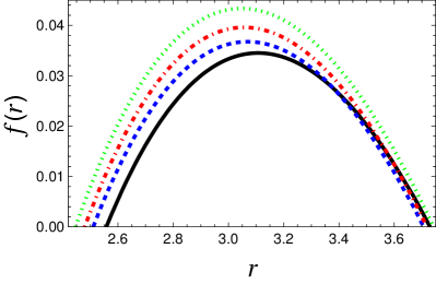
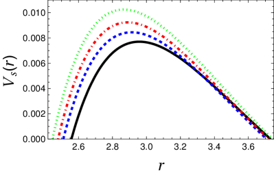
Figure 1: LEFT: Lapse function $f(r)$ vs radial coordinate $r$ for $M=1$ and $\Lambda_{0}=0.1$ in four different cases for the scale-dependent parameter $\epsilon$: i) $\epsilon=0$ (classical solution, solid black line), ii) $\epsilon=0.010$ (dashed blue line), iii) $\epsilon=0.015$ (dot-dashed red line), and finally iv) $\epsilon=0.020$ (dotted green line). RIGHT: Effective potential barrier $V_{s}(r)$ for the scalar case, taking $M=1$, $\Lambda_{0}=0.1$ and $l=1$ in four different cases of the scale-dependent parameter $\epsilon$ as follows: i) $\epsilon=0$ (solid black line), ii) $\epsilon=0.010$ (dashed blue line), iii) $\epsilon=0.015$ (dot-dashed red line), and finally iv) $\epsilon=0.020$ (dotted green line).

IV QNM spectra of SD Schwarzschild-de Sitter BH in the WKB approximation

Exact analytical calculations are always desirable, since it is only in this case where the complete parameter space can be fully explored. Regarding QN spectra of black holes, exact analytic expressions exist in very few cases, e.g. either when the effective potential barrier takes the form of the Pöschl-Teller potential potential ; ferrari ; lemos ; molina ; panotop1 , or when the radial part of the wave function may be recast into the Gauss’ hypergeometric function exact1 ; exact2 ; exact3 ; exact4 ; exact5 ; exact6 . More generically, over the years several different methods to compute the QNMs of black holes have been developed, such as the Frobenius method, generalization of the Frobenius series, fit and interpolation approach, method of continued fraction etc. For more details the interested reader may want to consult e.g. review3 . In particular, semi-analytical methods based on the Wentzel-Kramers-Brillouin (WKB) approximation wkb1 ; wkb2 ; wkb3 are among the most popular ones, and they have been extensively applied to several cases. For higher order WKB corrections, and recipes for simple, quick, efficient and accurate computations see Opala ; Konoplya:2019hlu ; RefExtra2 . For a partial list see for instance paper1 ; paper2 ; paper3 ; paper4 ; paper5 ; paper6 , and for more recent works paper7 ; paper8 ; paper9 ; paper10 ; Rincon:2018sgd ; Rincon:2020iwy , and references therein.

Within the WKB approximation the QN frequencies are computed by

$$\omega_{n}^{2}=V_{0}+(-2V_{0}^{\prime\prime})^{1/2}\Lambda(n)-i\nu(-2V_{0}^{\prime\prime})^{1/2}[1+\Omega(n)]$$ (53)

where $n=0,1,2...$ is the overtone number, $\nu=n+1/2$, $V_{0}$ is the maximum of the effective potential, $V_{0}^{\prime\prime}$ is the second derivative of the effective potential evaluated at the maximum, while $\Lambda(n),\Omega(n)$ are complicated expressions of $\nu$ and higher derivatives of the potential evaluated at the maximum, and can be seen e.g. in paper2 ; paper7 . Here we have used the Wolfram Mathematica wolfram code with WKB at any order from one to six, which has been presented in code , and it can be downloaded from https://g00.gl/hykYGL. It is known that within the WKB approach the best results are obtained for higher angular degrees and low overtone number, see e.g. the numerical values shown in Tables II, III, IV and V of Opala . Therefore in this work we shall consider $l=6,7,8,9,10$ and $n=0,1,2$ for the scalar and electromagnetic perturbations, while for Dirac perturbations we consider the fundamental mode of $\xi=7,8,9,10,11$.

Table 1: QN frequencies for scalar perturbations, setting $M=1$ and $\Lambda_{0}=0.1$ for three different values of the scale-dependent parameter $\epsilon$. For comparison reasons, we also show the frequencies of the classical geometry, i.e., when $\epsilon=0$. The modes are presented as follows: i) classical modes (without parenthesis), ii) scale-dependent modes with $\epsilon=0.01$ (in parenthesis), iii) scale-dependent modes with $\epsilon=0.015$ (in brackets), and finally iv) scale-dependent modes with $\epsilon=0.02$ (in curly brackets).

$n$	$l=6$	$l=7$	$l=8$	$l=9$	$l=10$
	0.39349  -0.0304656 i	0.454634  -0.030456 i	0.515703  -0.0304501 i	0.576729  -0.0304459 i	0.637722  -0.0304429 i
0	(0.411628  -0.0318694 i)	(0.475575  -0.0318598 i)	(0.539456  -0.0318531 i)	(0.603291  -0.0318484 i)	(0.667091  -0.0318451 i)
	[0.429689  -0.0332691 i]	[0.49644  -0.033258 i]	[0.563117  -0.0332507 i]	[0.629748  -0.0332455 i]	[0.696343  -0.0332418 i]
	{0.451879  -0.0349884 i }	{0.522067  -0.0349759 i }	{ 0.592181  -0.0349676 i }	{ 0.662247  -0.0349617 i }	{0.732275  -0.0349575 i}
	0.39318  -0.0914102 i	0.45444  -0.0913634 i	0.515507  -0.091351 i	0.576549  -0.0913392 i	0.637555  -0.0913304 i
1	(0.411359  -0.0956035 i)	(0.475308  -0.0955831 i)	(0.539219  -0.0955625 i)	(0.60309  -0.0955462 i)	(0.666899  -0.0955374 i)
	[0.429343  -0.0998119 i]	[0.496158  -0.099774 i]	[0.562849  -0.0997559 i]	[0.629518  -0.0997381 i]	[0.69613  -0.0997276 i]
	{0.451479  -0.104971 i}	{ 0.521721  -0.104932 i}	{0.59187  -0.104907 i}	{0.661979  -0.104887 i}	{ 0.732031  -0.104875 i }
	0.392421  -0.152449 i	0.454183  -0.152213 i	0.515138  -0.152246 i	0.576192  -0.152236 i	0.637204  -0.152227 i
2	(0.410945  -0.159274 i)	(0.474763  -0.159321 i)	(0.538728  -0.159287 i)	(0.602708  -0.159242 i)	(0.666495  -0.159241 i)
	[0.428659  -0.166365 i]	[0.495658  -0.166269 i]	[0.562294  -0.166278 i]	[0.629075  -0.16623 i]	[0.695693  -0.1662221 i]
	{0.45069  -0.174966 i }	{0.52103  -0.174901 i }	{ 0.591224  -0.174868 i }	{ 0.66146  -0.174815 i }	{ 0.731548  -0.174796 i }

Table 2: QN frequencies for electromagnetic perturbations, setting $M=1$ and $\Lambda_{0}=0.1$ for three different values of the scale-dependent parameter $\epsilon$. For comparison reasons, we also show the frequencies of the classical geometry, i.e., when $\epsilon=0$. The modes are presented as follows: i) classical modes (without parenthesis), ii) scale-dependent modes with $\epsilon=0.01$ (in parenthesis), iii) scale-dependent modes with $\epsilon=0.015$ (in brackets), and finally iv) scale-dependent modes with $\epsilon=0.02$ (in curly brackets).

$n$	$l=6$	$l=7$	$l=8$	$l=9$	$l=10$
	0.393183  -0.030421 i	0.454364  -0.0304228 i	0.515465  -0.0304243 i	0.576515  -0.0304253 i	0.63753  -0.0304259 i
0	(0.411284  -0.0318204 i)	(0.475275  -0.031823 i)	0.539191  -0.0318245 i)	(0.603054  -0.0318256 i)	(0.666877  -0.0318264 i)
	[0.429299  -0.0332147 i]	[0.496101  -0.0332172 i]	[0.56282  -0.033219 i]	[0.629482  -0.0332201 i]	[0.696103  -0.033221 i]
	{0.451433 -0.0349266 i}	{0.521681 -0.0349295 i}	{0.591841 -0.0349315 i}	{0.661941 -0.0349329 i}	{0.731999 -0.0349339 i}
	0.392931  -0.091264 i	0.454167  -0.0912645 i	0.51527  -0.0912737 i	0.576333   -0.0912776 i	0.63737, -0.0912787 i
1	(0.41105  -0.0954503 i)	( 0.475014  -0.095472 i)	(0.538965  -0.0954752 i)	(0.602855  -0.0954776 i)	(0.666688  -0.095481 i)
	[0.428948  -0.0996512 i]	[0.495802  -0.0996562 i]	[0.562559  -0.0996598 i]	[0.629254  -0.0996619 i]	[0.695893  -0.0996648 i]
	{0.45103  -0.104787 i}	{0.521339  -0.104793 i}	{0.591542  -0.104797 i}	{0.66167  -0.104802 i }	{0.731757  -0.104804 i }
	0.392453  -0.1521 i	0.453873  -0.15206 i	0.514898  -0.152121 i	0.575956  -0.152139 i	0.637055  -0.152133 i
2	(0.410791  -0.158967 i)	(0.474483  -0.159133 i)	(0.538515  -0.15913)	(0.602473  -0.159128 i)	(0.666297  -0.1591451 i)
	[0.428199  -0.166127 i]	[0.495176  -0.166117 i]	[0.562026  -0.166112 i]	[0.628805  -0.166106 i]	[0.695466  -0.166115 i]
	{0.450181  -0.174687 i }	{0.520641  -0.174673 i }	{0.590941  -0.174673 i }	{0.661112  -0.174683 i}	{0.731273  -0.174679 i }

Table 3: Dirac perturbations with $V_{+}$: Fundamental mode $n=0$ for $\xi=7,8,9,10,11$.

	QN frequencies for Dirac perturbations
$\xi$	$\epsilon=0$	$\epsilon=0.001$	$\epsilon=0.002$	$\epsilon=0.003$
7	0.4260-0.0304 i	0.4277-0.0303 i	0.4281-0.0304 i	0.4307-0.0304 i
8	0.4868-0.0304 i	0.4870-0.0305 i	0.4879-0.0305 i	0.4897-0.0306 i
9	0.5477-0.0304 i	0.5484-0.0304 i	0.5489-0.0305 i	0.5510-0.0306 i
10	0.6085-0.0304 i	0.6092-0.0304 i	0.6101-0.0305 i	0.6119-0.0306 i
11	0.6694-0.0304 i	0.6699-0.0305 i	0.6711-0.0305 i	0.6731-0.0306 i

The obtained QNMs are summarized in Tables 1, 2 and 3, and they are pictorially shown in Figures  2 and 3. We recall that the information on the stability of the modes is encoded into the sign of the imaginary part of the QN modes. In particular, given the time dependence, $\sim e^{-i\omega t}$, it is easy to verify that when $\omega_{I}>0$ the perturbation grows exponentially (unstable mode), whereas when $\omega_{I}<0$ the perturbation decays exponentially (stable mode). Furthermore, the real part of the modes determines the frequency of the oscillation, $\nu=\omega/(2\pi)$, while the inverse of the absolute value of the imaginary part of the modes determines the damping time, $\tau=1/|\omega_{I}|$. Those imply that when the real part increases the modes oscillate faster, while when the absolute value of the imaginary part increases the modes decay faster.

Our results show i) that all modes are found to be stable, ii) the SD spectra follow the pattern of the classical spectra regarding the impact of the overtone number and the angular degree, and iii) for given $l,n$ both the real part and the absolute value of the imaginary part of the frequencies increase with the parameter $\epsilon$ that measures the deviation from the classical geometry. Therefore, in the framework of scale-dependent gravity the QN modes are characterized by a lower damping time, they oscillate faster and they decay faster than their classical counterparts. Moreover, modes characterized by a larger damping time will dominate at later times during the quasinormal ringing.

Regarding future work, it would be both challenging and interesting to compute the QNMs for gravitational perturbations, since they may serve as a distinguisher between GR and alternative theories of gravity, see e.g. Bhattacharyya:2017tyc . There it was shown that contrary to what happens in GR, where axial and polar modes share equal amounts of radiation, this does not hold in $f(R)$ theories of gravity. Moreover, the strong cosmic censorship conjecture Penrose:1969pc ; Dafermos:2012np is a hot topic in black hole physics. It would be interesting to see if the conclusions obtained in GR for geometries with a positive cosmological constant (see e.g. Mellor:1989ac ; Dias:2018ynt and references therein) are respected or violated in SD gravity. We hope to be able to address those issues in a forthcoming article.

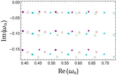
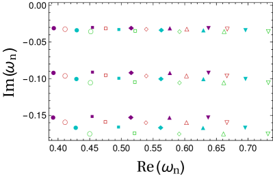
Figure 2: Quasinormal modes $\omega_{n}\equiv\omega_{R}+i\omega_{I}$. LEFT: (Scalar field) $\text{Im}(\omega_{n})$ versus $\text{Re}(\omega_{n})$ for $M=1$ and $\Lambda_{0}=0.1$ in five different cases: i) $l=6$ (points), ii) $l=7$ (squares), iii) $l=8$ (rhombus), iv) $l=9$ (triangles), and v) $l=10$ (inverted triangles) RIGHT: Same as in the left panel, but for the Maxwell field. Also notice the color code, i.e., i) purple for the classical case, ii) red for $\epsilon=0.01$, iii) cyan for $\epsilon=0.015$ and finally, iv) green for $\epsilon=0.02$. From top to down, we consider from $n=0$ to $n=2$.

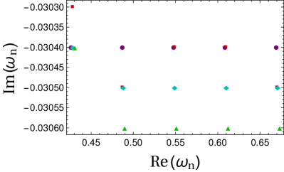
Figure 3: Quasinormal modes (Dirac field) $\omega_{n}\equiv\omega_{R}+i\omega_{I}$ for the potential with the plus sign, $V_{+}$. $\text{Im}(\omega_{n})$ versus $\text{Re}(\omega_{n})$ for $M=1$ and $\Lambda_{0}=0.1$ in five different cases of $\xi$. From left to right, we consider from $\xi=7$ to $\xi=11$. Also notice the color code, i.e., i) purple points for the classical case, ii) red squares for $\epsilon=0.001$, iii) cyan rhombus for $\epsilon=0.002$ and finally, iv) green triangles for $\epsilon=0.003$.

V Conclusions

Summarizing our work, in the present article we have studied the quasinormal spectra for massless scalar, Dirac as well as electromagnetic perturbations of four-dimensional scale-dependent Schwarzschild-de Sitter black holes. After reviewing the basic effective field equations of scale-dependent gravity, we perturbed the black hole with a test massless field, and we investigated its propagation into a fixed gravitational background. The wave equations with the corresponding effective potential barrier were presented. The QN frequencies were numerically computed employing the WKB method of 6th order. For better visualization, we showed on the ($\omega_{R}-\omega_{I}$) plane the impact on the spectrum of the overtone number, the angular degree and the scale-dependent parameter $\epsilon$. All modes were found to be stable. Our main results indicate that i) when $l$ increases, the modes corresponding to the scalar and Maxwell field decreases, ii) when $\epsilon$ increases, for a given $l$, the modes for the scalar and Maxwell field decrease, and finally iii) when $n$ increases, for a given $\epsilon$ and $l$, both the real and the imaginary part of all modes decrease. Finally, within SD gravity the QN modes oscillate and decay faster in comparison with their classical counterparts.

Acknowlegements

We are grateful to the anonymous reviewer for useful comments and suggestions. The author G. P. thanks the Fundação para a Ciência e Tecnologia (FCT), Portugal, for the financial support to the Center for Astrophysics and Gravitation-CENTRA, Instituto Superior Técnico, Universidade de Lisboa, through the Project No. UIDB/00099/2020. The author Á. R. acknowledges DI-VRIEA for financial support through Proyecto Postdoctorado 2019 VRIEA-PUCV.

References

- [1] Albert Einstein. The Foundation of the General Theory of Relativity. Annalen Phys., 49(7):769–822, 1916.
- [2] Slava G. Turyshev. Experimental Tests of General Relativity. Ann. Rev. Nucl. Part. Sci., 58:207–248, 2008.
- [3] Clifford M. Will. The Confrontation between General Relativity and Experiment. Living Rev. Rel., 17:4, 2014.
- [4] Estelle Asmodelle. Tests of General Relativity: A Review. Bachelor thesis, Central Lancashire U., 2017.
- [5] Kazunori Akiyama et al. First M87 Event Horizon Telescope Results. I. The Shadow of the Supermassive Black Hole. Astrophys. J., 875(1):L1, 2019.
- [6] Kazunori Akiyama et al. First M87 Event Horizon Telescope Results. II. Array and Instrumentation. Astrophys. J., 875(1):L2, 2019.
- [7] Kazunori Akiyama et al. First M87 Event Horizon Telescope Results. III. Data Processing and Calibration. Astrophys. J., 875(1):L3, 2019.
- [8] Kazunori Akiyama et al. First M87 Event Horizon Telescope Results. IV. Imaging the Central Supermassive Black Hole. Astrophys. J., 875(1):L4, 2019.
- [9] Kazunori Akiyama et al. First M87 Event Horizon Telescope Results. V. Physical Origin of the Asymmetric Ring. Astrophys. J., 875(1):L5, 2019.
- [10] Kazunori Akiyama et al. First M87 Event Horizon Telescope Results. VI. The Shadow and Mass of the Central Black Hole. Astrophys. J., 875(1):L6, 2019.
- [11] B. P. Abbott et al. Observation of Gravitational Waves from a Binary Black Hole Merger. Phys. Rev. Lett., 116(6):061102, 2016.
- [12] B. P. Abbott et al. GW151226: Observation of Gravitational Waves from a 22-Solar-Mass Binary Black Hole Coalescence. Phys. Rev. Lett., 116(24):241103, 2016.
- [13] Benjamin P. Abbott et al. GW170104: Observation of a 50-Solar-Mass Binary Black Hole Coalescence at Redshift 0.2. Phys. Rev. Lett., 118(22):221101, 2017. [Erratum: Phys. Rev. Lett.121,no.12,129901(2018)].
- [14] B. P. Abbott et al. GW170814: A Three-Detector Observation of Gravitational Waves from a Binary Black Hole Coalescence. Phys. Rev. Lett., 119(14):141101, 2017.
- [15] B.. P.. Abbott et al. GW170608: Observation of a 19-solar-mass Binary Black Hole Coalescence. Astrophys. J., 851(2):L35, 2017.
- [16] Ignatios Antoniadis, E. Kiritsis, and T.N. Tomaras. A D-brane alternative to unification. Phys. Lett. B, 486:186–193, 2000.
- [17] A. Mironov, A. Morozov, and T.N. Tomaras. Can centauros or chirons be the first observations of evaporating mini black holes? Int. J. Mod. Phys. A, 24:4097–4115, 2009.
- [18] Alex Casanova and Euro Spallucci. TeV mini black hole decay at future colliders. Class. Quant. Grav., 23:R45–R62, 2006.
- [19] John F. Donoghue. General relativity as an effective field theory: The leading quantum corrections. Phys. Rev. D, 50:3874–3888, 1994.
- [20] Carlos Contreras, Benjamin Koch, and Paola Rioseco. Black hole solution for scale-dependent gravitational couplings and the corresponding coupling flow. Class. Quant. Grav., 30:175009, 2013.
- [21] Benjamin Koch and Paola Rioseco. Black Hole Solutions for Scale Dependent Couplings: The de Sitter and the Reissner-Nordström Case. Class. Quant. Grav., 33:035002, 2016.
- [22] Benjamin Koch, Ignacio A. Reyes, and Ángel Rincón. A scale dependent black hole in three-dimensional space–time. Class. Quant. Grav., 33(22):225010, 2016.
- [23] Ángel Rincón and Benjamin Koch. On the null energy condition in scale dependent frameworks with spherical symmetry. J. Phys. Conf. Ser., 1043(1):012015, 2018.
- [24] A. Hernández-Arboleda, Á. Rincón, B. Koch, E. Contreras, and P. Bargueño. Preliminary test of cosmological models in the scale-dependent scenario. 2018.
- [25] Ernesto Contreras, Ángel Rincón, and J. M. Ramírez-Velasquez. Relativistic dust accretion onto a scale–dependent polytropic black hole. Eur. Phys. J., C79(1):53, 2019.
- [26] Felipe Canales, Benjamin Koch, Cristobal Laporte, and Angel Rincon. Cosmological constant problem: deflation during inflation. 2018.
- [27] Ángel Rincón and J. R. Villanueva. The Sagnac effect on a scale-dependent rotating BTZ black hole background. 2019.
- [28] Ángel Rincón and Benjamin Koch. Scale-dependent rotating BTZ black hole. Eur. Phys. J., C78(12):1022, 2018.
- [29] E. Contreras, Á. Rincón, and P. Bargueño. Five-Dimensional Scale-Dependent Black Holes with Constant Curvature and Solv Horizons. Eur. Phys. J. C, 80(5):367, 2020.
- [30] Mohsen Fathi, Ángel Rincón, and J.R. Villanueva. Photon trajectories on a first order scale-dependent static BTZ black hole. Class. Quant. Grav., 37(7):075004, 2020.
- [31] Grigoris Panotopoulos, Ángel Rincón, and Ilídio Lopes. Interior solutions of relativistic stars in the scale-dependent scenario. Eur. Phys. J. C, 80(4):318, 2020.
- [32] Ernesto Contreras and Pedro Bargueño. A self-sustained traversable scale-dependent wormhole. Int. J. Mod. Phys., D27(09):1850101, 2018.
- [33] Carlos M. Sendra. Regular scale-dependent black holes as gravitational lenses. Gen. Rel. Grav., 51(7):83, 2019.
- [34] Ángel Rincón, Ernesto Contreras, Pedro Bargueño, Benjamin Koch, Grigorios Panotopoulos, and Alejandro Hernández-Arboleda. Scale dependent three-dimensional charged black holes in linear and non-linear electrodynamics. Eur. Phys. J. C, 77(7):494, 2017.
- [35] Ángel Rincón and Grigoris Panotopoulos. Quasinormal modes of scale dependent black holes in ( 1+2 )-dimensional Einstein-power-Maxwell theory. Phys. Rev. D, 97(2):024027, 2018.
- [36] Ernesto Contreras, Ángel Rincón, Benjamin Koch, and Pedro Bargueño. Scale-dependent polytropic black hole. Eur. Phys. J. C, 78(3):246, 2018.
- [37] Ángel Rincón and Benjamin Koch. Scale-dependent BTZ black hole. Eur. Phys. J. C, 78(12):1022, 2018.
- [38] Ángel Rincón, Ernesto Contreras, Pedro Bargueño, Benjamin Koch, and Grigorios Panotopoulos. Scale-dependent ( )-dimensional electrically charged black holes in Einstein-power-Maxwell theory. Eur. Phys. J. C, 78(8):641, 2018.
- [39] Ángel Rincón, Ernesto Contreras, Pedro Bargueño, and Benjamin Koch. Scale-dependent planar Anti-de Sitter black hole. Eur. Phys. J. Plus, 134(11):557, 2019.
- [40] Ernesto Contreras, Ángel Rincón, Grigoris Panotopoulos, Pedro Bargueño, and Benjamin Koch. Black hole shadow of a rotating scale–dependent black hole. Phys. Rev. D, 101(6):064053, 2020.
- [41] Alfio Bonanno and Martin Reuter. Renormalization group improved black hole space-times. Phys. Rev., D62:043008, 2000.
- [42] A. Bonanno and M. Reuter. Cosmology of the Planck era from a renormalization group for quantum gravity. Phys. Rev., D65:043508, 2002.
- [43] M. Reuter and H. Weyer. Renormalization group improved gravitational actions: A Brans-Dicke approach. Phys. Rev., D69:104022, 2004.
- [44] Benjamin Koch and Frank Saueressig. Black holes within Asymptotic Safety. Int. J. Mod. Phys. A, 29(8):1430011, 2014.
- [45] Cristopher González and Benjamin Koch. Improved Reissner–Nordström–(A)dS black hole in asymptotic safety. Int. J. Mod. Phys. A, 31(26):1650141, 2016.
- [46] Tullio Regge and John A. Wheeler. Stability of a Schwarzschild singularity. Phys. Rev., 108:1063–1069, 1957.
- [47] Frank J. Zerilli. Effective potential for even parity Regge-Wheeler gravitational perturbation equations. Phys. Rev. Lett., 24:737–738, 1970.
- [48] F. J. Zerilli. Gravitational field of a particle falling in a schwarzschild geometry analyzed in tensor harmonics. Phys. Rev., D2:2141–2160, 1970.
- [49] F. J. Zerilli. Perturbation analysis for gravitational and electromagnetic radiation in a reissner-nordstroem geometry. Phys. Rev., D9:860–868, 1974.
- [50] Vincent Moncrief. Gauge-invariant perturbations of Reissner-Nordstrom black holes. Phys. Rev., D12:1526–1537, 1975.
- [51] S. A. Teukolsky. Rotating black holes - separable wave equations for gravitational and electromagnetic perturbations. Phys. Rev. Lett., 29:1114–1118, 1972.
- [52] Kostas D. Kokkotas and Bernd G. Schmidt. Quasinormal modes of stars and black holes. Living Rev. Rel., 2:2, 1999.
- [53] Emanuele Berti, Vitor Cardoso, and Andrei O. Starinets. Quasinormal modes of black holes and black branes. Class. Quant. Grav., 26:163001, 2009.
- [54] R. A. Konoplya and A. Zhidenko. Quasinormal modes of black holes: From astrophysics to string theory. Rev. Mod. Phys., 83:793–836, 2011.
- [55] Subrahmanyan Chandrasekhar. The mathematical theory of black holes. In Oxford, UK: Clarendon (1992) 646 p., OXFORD, UK: CLARENDON (1985) 646 P., 1985.
- [56] Adam G. Riess et al. Observational evidence from supernovae for an accelerating universe and a cosmological constant. Astron. J., 116:1009–1038, 1998.
- [57] S. Perlmutter et al. Measurements of and from 42 high redshift supernovae. Astrophys. J., 517:565–586, 1999.
- [58] Vitor Cardoso and Jose P. S. Lemos. Quasinormal modes of the near extremal Schwarzschild-de Sitter black hole. Phys. Rev., D67:084020, 2003.
- [59] C. Molina. Quasinormal modes of d-dimensional spherical black holes with near extreme cosmological constant. Phys. Rev., D68:064007, 2003.
- [60] A. Zhidenko. Quasinormal modes of Schwarzschild de Sitter black holes. Class. Quant. Grav., 21:273–280, 2004.
- [61] R.A. Konoplya and A. Zhidenko. High overtones of Schwarzschild-de Sitter quasinormal spectrum. JHEP, 06:037, 2004.
- [62] A. Lopez-Ortega. Quasinormal modes of D-dimensional de Sitter spacetime. Gen. Rel. Grav., 38:1565–1591, 2006.
- [63] Hideo Kodama and Akihiro Ishibashi. A Master equation for gravitational perturbations of maximally symmetric black holes in higher dimensions. Prog. Theor. Phys., 110:701–722, 2003.
- [64] Grigoris Panotopoulos. Electromagnetic quasinormal modes of the nearly-extremal higher-dimensional Schwarzschild–de Sitter black hole. Mod. Phys. Lett., A33(23):1850130, 2018.
- [65] Luís C. B. Crispino, Atsushi Higuchi, Ednilton S. Oliveira, and Jorge V. Rocha. Greybody factors for nonminimally coupled scalar fields in Schwarzschild–de Sitter spacetime. Phys. Rev., D87:104034, 2013.
- [66] Panagiota Kanti, Thomas Pappas, and Nikolaos Pappas. Greybody factors for scalar fields emitted by a higher-dimensional Schwarzschild–de Sitter black hole. Phys. Rev., D90(12):124077, 2014.
- [67] T. Pappas, P. Kanti, and N. Pappas. Hawking radiation spectra for scalar fields by a higher-dimensional schwarzschild–de sitter black hole. Phys. Rev. D, 94:024035, Jul 2016.
- [68] Kyriakos Destounis. Charged Fermions and Strong Cosmic Censorship. Phys. Lett. B, 795:211–219, 2019.
- [69] Felix Finster, Joel Smoller, and Shing-Tung Yau. Nonexistence of time periodic solutions of the Dirac equation in a Reissner-Nordstrom black hole background. J. Math. Phys., 41:2173–2194, 2000.
- [70] Fred Cooper, Avinash Khare, and Uday Sukhatme. Supersymmetry and quantum mechanics. Phys. Rept., 251:267–385, 1995.
- [71] Vitor Cardoso and Jose P. S. Lemos. Quasinormal modes of Schwarzschild anti-de Sitter black holes: Electromagnetic and gravitational perturbations. Phys. Rev., D64:084017, 2001.
- [72] F. R. Tangherlini. Schwarzschild field in n dimensions and the dimensionality of space problem. Nuovo Cim., 27:636–651, 1963.
- [73] Christof Wetterich. Exact evolution equation for the effective potential. Phys. Lett., B301:90–94, 1993.
- [74] Djamel Dou and Roberto Percacci. The running gravitational couplings. Class. Quant. Grav., 15:3449–3468, 1998.
- [75] Wataru Souma. Nontrivial ultraviolet fixed point in quantum gravity. Prog. Theor. Phys., 102:181–195, 1999.
- [76] M. Reuter and Frank Saueressig. Renormalization group flow of quantum gravity in the Einstein-Hilbert truncation. Phys. Rev., D65:065016, 2002.
- [77] G. Poschl and E. Teller. Bemerkungen zur Quantenmechanik des anharmonischen Oszillators. Z. Phys., 83:143–151, 1933.
- [78] Valeria Ferrari and Bahram Mashhoon. New approach to the quasinormal modes of a black hole. Phys. Rev., D30:295–304, 1984.
- [79] Danny Birmingham. Choptuik scaling and quasinormal modes in the AdS / CFT correspondence. Phys. Rev., D64:064024, 2001.
- [80] Sharmanthie Fernando. Quasinormal modes of charged dilaton black holes in (2+1)-dimensions. Gen. Rel. Grav., 36:71–82, 2004.
- [81] Sharmanthie Fernando. Quasinormal modes of charged scalars around dilaton black holes in 2+1 dimensions: Exact frequencies. Phys. Rev., D77:124005, 2008.
- [82] Kyriakos Destounis, Grigoris Panotopoulos, and Ángel Rincón. Stability under scalar perturbations and quasinormal modes of 4D Einstein–Born–Infeld dilaton spacetime: exact spectrum. Eur. Phys. J., C78(2):139, 2018.
- [83] Alï Ovgün and Kimet Jusufi. Quasinormal Modes and Greybody Factors of gravity minimally coupled to a cloud of strings in Dimensions. Annals Phys., 395:138–151, 2018.
- [84] Ángel Rincón and Grigoris Panotopoulos. Greybody factors and quasinormal modes for a nonminimally coupled scalar field in a cloud of strings in (2+1)-dimensional background. Eur. Phys. J., C78(10):858, 2018.
- [85] Bernard F. Schutz and Clifford M. Will. BLACK HOLE NORMAL MODES: A SEMIANALYTIC APPROACH. Astrophys. J., 291:L33–L36, 1985.
- [86] Sai Iyer and Clifford M. Will. Black Hole Normal Modes: A WKB Approach. 1. Foundations and Application of a Higher Order WKB Analysis of Potential Barrier Scattering. Phys. Rev., D35:3621, 1987.
- [87] R. A. Konoplya. Quasinormal behavior of the d-dimensional Schwarzschild black hole and higher order WKB approach. Phys. Rev., D68:024018, 2003.
- [88] Jerzy Matyjasek and Michał Opala. Quasinormal modes of black holes. The improved semianalytic approach. Phys. Rev., D96(2):024011, 2017.
- [89] R. A. Konoplya, A. Zhidenko, and A. F. Zinhailo. Higher order WKB formula for quasinormal modes and grey-body factors: recipes for quick and accurate calculations. Class. Quant. Grav., 36:155002, 2019.
- [90] Yasuyuki Hatsuda. Quasinormal modes of black holes and Borel summation. 2019.
- [91] Sai Iyer. BLACK HOLE NORMAL MODES: A WKB APPROACH. 2. SCHWARZSCHILD BLACK HOLES. Phys. Rev., D35:3632, 1987.
- [92] K. D. Kokkotas and Bernard F. Schutz. Black Hole Normal Modes: A WKB Approach. 3. The Reissner-Nordstrom Black Hole. Phys. Rev., D37:3378–3387, 1988.
- [93] Edward Seidel and Sai Iyer. BLACK HOLE NORMAL MODES: A WKB APPROACH. 4. KERR BLACK HOLES. Phys. Rev., D41:374–382, 1990.
- [94] Roman Konoplya. Quasinormal modes of the charged black hole in Gauss-Bonnet gravity. Phys. Rev., D71:024038, 2005.
- [95] Sharmanthie Fernando and Chad Holbrook. Stability and quasi normal modes of charged black holes in Born-Infeld gravity. Int. J. Theor. Phys., 45:1630–1645, 2006.
- [96] Sayan K. Chakrabarti. Quasinormal modes of tensor and vector type perturbation of Gauss Bonnet black hole using third order WKB approach. Gen. Rel. Grav., 39:567–582, 2007.
- [97] Sharmanthie Fernando and Juan Correa. Quasinormal Modes of Bardeen Black Hole: Scalar Perturbations. Phys. Rev., D86:064039, 2012.
- [98] Victor Santos, R. V. Maluf, and C. A. S. Almeida. Quasinormal frequencies of self-dual black holes. Phys. Rev., D93(8):084047, 2016.
- [99] Jose Luis Blázquez-Salcedo, Fech Scen Khoo, and Jutta Kunz. Quasinormal modes of Einstein-Gauss-Bonnet-dilaton black holes. Phys. Rev., D96(6):064008, 2017.
- [100] Grigoris Panotopoulos and Ángel Rincón. Quasinormal modes of black holes in Einstein-power-Maxwell theory. Int. J. Mod. Phys., D27(03):1850034, 2017.
- [101] Ángel Rincón and Grigoris Panotopoulos. Quasinormal modes of scale dependent black holes in ( 1+2 )-dimensional Einstein-power-Maxwell theory. Phys. Rev., D97(2):024027, 2018.
- [102] Ángel Rincón and Grigoris Panotopoulos. Quasinormal modes of an improved Schwarzschild black hole. Phys. Dark Univ., 30:100639, 2020.
- [103] Wolfram alpha software. http://www.wolfram.com. Accessed: 2019-06-11.
- [104] R. A. Konoplya and A. Zhidenko. Passage of radiation through wormholes of arbitrary shape. Phys. Rev., D81:124036, 2010.
- [105] Soham Bhattacharyya and S. Shankaranarayanan. Quasinormal modes as a distinguisher between general relativity and f(R) gravity. Phys. Rev. D, 96(6):064044, 2017.
- [106] R. Penrose. Gravitational collapse: The role of general relativity. Riv. Nuovo Cim., 1:252–276, 1969.
- [107] Mihalis Dafermos. Black holes without spacelike singularities. Commun. Math. Phys., 332:729–757, 2014.
- [108] Felicity Mellor and Ian Moss. Stability of Black Holes in De Sitter Space. Phys. Rev. D, 41:403, 1990.
- [109] Oscar J.C. Dias, Felicity C. Eperon, Harvey S. Reall, and Jorge E. Santos. Strong cosmic censorship in de Sitter space. Phys. Rev. D, 97(10):104060, 2018.