Abstract

Quantization implies independent degrees of freedom that do not appear in the classical theory, given by fluctuations, correlations, and higher moments of a state. A systematic derivation of the resulting dynamical systems is presented here in a cosmological application for near-Gaussian states of a single-field inflation model. As a consequence, single-field Higgs inflation is made viable observationally by becoming a multi-field model with a specific potential for a fluctuation field interacting with the inflaton expectation value. Crucially, non-adiabatic methods of semiclassical quantum dynamics reveal important phases that can set suitable initial conditions for slow-roll inflation (in combination with the uncertainty relation), and then end inflation after the observationally preferred number of $e$-folds. New parameters in the interaction potential are derived from properties of the underlying background state, demonstrating how background non-Gaussianity can affect observational features of inflation or, conversely, how observations may be used to understand the quantum state of the inflaton.

1 Introduction

It is a natural requirement that self-consistent inflationary models should be largely independent of the high energy quantum gravity theory, viewed in an effective field theory framework. However, an exact decoupling of scales relevant for inflation from high-energy modes can happen only if the low-energy Lagrangian consists entirely of terms that are renormalizable using Wilsonian effective actions. This condition restricts single-field models of inflation to be of chaotic type with quartic potentials.

If the inflationary action contains terms beyond mass-dimension four, then the theory is liable to be affected by as yet unknown high-energy physics. In fact, one even has to rely on ultraviolet physics in order to derive a suitable higher-order form of the potential. In common single-field inflation, this problem can rarely be avoided as the models preferred by observations [1] depend crucially on non-renormalizable terms in the potential, as for instance in Starobinsky inflation [2]. Fundamentally, such terms have to be understood as remnants in an effective description of some underlying theory of gravity and matter, such as quantum gravity or string theory, but specific top-down justifications of suitable forms of the potential are usually hard to come by.

Alternatively, if chaotic-type potentials, which have been ruled out by data as single-field models, can somehow be resurrected, then the burden of explaining these potentials does not have to fall on quantum gravity. Motivated by this observation, we begin with a Higgs-inspired classical potential,

$$V_{\rm cl}(\psi)=M^{4}\left(1-2\dfrac{\psi^{2}}{v^{2}}+\dfrac{\psi^{4}}{v^{4}}\right)$$ (1)

with two parameters, $M$ and $v$, assumed to be positive. While the only known scalar to have been discovered to date is the standard-model Higgs particle, it is well-known that this type of a inflaton potential, by itself, is found to be inconsistent with cosmological observations. To make matters worse, even renormalization-group improvements do not suffice to make Higgs-like potentials compatible with data [3, 4, 5]. The only observationally consistent formulations proposed up until now have been based on a scalar field non-minimally coupled to the Ricci scalar [6, 7], modifying the kinetic term of the Higgs field. Non-minimal coupling terms, however, mean that one is forced to modify the nature of the standard model at high energies [8], amongst other issues [9].

In the present work, we will preserve the simple nature of a minimally coupled field with a quartic classical potential (1). Applying a canonical formalism of effective theory which, crucially, remains valid in non-adiabatic regimes, the classical potential will be quantum extended to a two-field model with a specific potential derived from (1). The second field, $\varphi$, represents quantum fluctuations of the background inflaton, $\psi$. As such, it is subject to uncertainty relations that will be used to obtain important lower bounds on its initial value. Initial evolution is then non-adiabatic, but it automatically sets the stage for a long slow-roll phase (in a so-called waterfall regime of the two-field model) that is consistent with observational constraints. A final non-adiabatic phase automatically ends inflation with just the right number of $e$-folds in a large region of the parameter space.

Coefficients of the two-field potential are determined by the same two parameters, $M$ and $v$, that appear in the single-field model (1). In addition, there are new coefficients derived from moments of the inflaton state, such as parameters for non-Gaussianity of the background state. In inflation models, this is a new kind of non-Gaussianity different from what one usually refers to in primordial fluctuations during inflation. In our case, non-Gaussianity is present already in the wave function of the homogeneous quantum inflaton field (referred to here as the background state), and not only in the perturbation spectrum. It is therefore possible to put constraints on the two-field potential based on known properties of states, or conversely, to determine conditions on suitable inflaton states based on observational constraints. An important finding is that constraints on the spectral index, its running, and the tensor-to-scalar ratio prefer small background non-Gaussianity.

In Section 2, we present a review of relevant methods of non-adiabatic quantum dynamics, which have appeared in various forms in fields as diverse as quantum field theory, quantum chaos, quantum chemistry, and quantum cosmology. The same section presents a comparison with Gaussian methods and shows how non-adiabatic dynamics can include non-Gaussian states. These methods are applied to cosmology in Section 3, focusing on Higgs-like inflation. The results are, however, more general and can easily be adapted to any potential. This section will demonstrate the importance of going beyond Gaussian dynamics, including higher-order moments, and maintaining non-adiabatic regimes. A detailed cosmological analysis, including numerical simulations and analytical approximations, is performed in Section 4, where observational implications are discussed. The derivations in the present paper justify the more concise physical discussion presented in [10].

2 Canonical effective potentials

Our construction is based on canonical effective methods for non-adiabatic quantum dynamics, which in a leading-order treatment has appeared several times independently in various fields [11, 12, 13, 14, 15, 16], including quantum chaos, quantum chemistry, and quantum cosmology, but has only recently been worked out to higher orders using systematic methods of Poisson manifolds [17, 18]. While higher orders go beyond Gaussian dynamics, the leading-order effects are closely related to Gaussian approximations and can therefore be used for an illustration of the method.

2.1 Relation to the time-dependent variational principle

In order to illustrate our claim that quantum fluctuations can provide an independent degree of freedom that can influence the inflationary dynamics, we first consider a canonical formulation of the time-dependent variational principle for Gaussian states.

The most general parametrization of Gaussian fluctuations around the homogeneous field $\psi$ can be represented by the wave function [11]

$$\Psi(\psi^{\prime}|\psi,\pi_{\psi},\varphi,\pi_{\varphi}) = \frac{1}{\left(2\pi\varphi^{2}\right)^{1/4}}\exp\left(-{\textstyle\frac{1}{4}}\varphi^{-2}(1-2i\varphi\pi_{\varphi})(\psi^{\prime}-\psi)^{2}\right)$$ (2)

$$\qquad\qquad\times\exp(i\pi_{\psi}(\psi^{\prime}-\psi))\exp(-{\textstyle\frac{1}{2}}i\varphi\pi_{\varphi})\,.$$

The notation is such that $\Psi$ is a wave function depending on $\psi^{\prime}$ for any choice of the parameters $\psi$, $\pi_{\psi}$, $\varphi$ and $\pi_{\varphi}$. Despite its lengthy form, this variational wave function has some useful properties: It is normalized, $\langle\Psi|\Psi\rangle=1$, and has basic expectation values

$$\langle\Psi|\hat{\psi}|\Psi\rangle=\psi\quad,\quad\langle\Psi|\hat{\pi}_{\psi}|\Psi\rangle=\pi_{\psi}$$ (3)

and variances

$$\langle\Psi|(\hat{\psi}-\psi)^{2}|\Psi\rangle=\varphi^{2}\quad,\quad\langle\Psi|(\hat{\pi}_{\psi}-\pi_{\psi})^{2}|\Psi\rangle=\pi_{\varphi}^{2}+\frac{1}{4\varphi^{2}}$$ (4)

where operators are defined with respect to the dependence of $\Psi$ on $\psi^{\prime}$. Moreover, $\Psi$ obeys the conditions

$$i\langle\Psi|\partial/\partial\psi|\Psi\rangle=\pi_{\psi}\quad \quad i\langle\Psi|\partial/\partial\varphi|\Psi\rangle=\pi_{\varphi}$$ , (5)

$$\langle\Psi|\partial/\partial\pi_{\psi}|\Psi\rangle=0\quad \quad\langle\Psi|\partial/\partial\pi_{\varphi}|\Psi\rangle=0\,.$$ , (6)

The equations of motion for the variational parameters, $\psi$, $\varphi$, $\pi_{\psi}$ and $\pi_{\varphi}$, are given by the variation of the action

$$S = \int{\rm d}t\left\langle\Psi\left|\left(i\partial_{t}-\hat{H}\right)\right|\Psi\right\rangle$$ (7)

$$= \int{\rm d}t\left(i\dot{\psi}\left\langle\Psi|\partial/\partial\psi|\Psi\right\rangle+i\dot{\varphi}\left\langle\Psi|\partial/\partial\varphi|\Psi\right\rangle-\langle\Psi|\hat{H}|\Psi\rangle\right)$$

using the chain rule. The identities obeyed by $\Psi$ therefore allow us to write the action in canonical form,

$$S=\int{\rm d}t\left(\dot{\psi}\pi_{\psi}+\dot{\varphi}\pi_{\varphi}-H_{\rm G}\right)$$ (8)

where we defined the Gaussian Hamiltonian $H_{\rm G}=\langle\Psi|\hat{H}|\Psi\rangle$. The variation of this action gives Hamilton’s equations

$$\dot{\psi}=\frac{\partial H_{\rm G}}{\partial\pi_{\psi}}\quad,\quad\dot{\pi}_{\psi}=-\frac{\partial H_{\rm G}}{\partial\psi}\quad,\quad\dot{\varphi}=\frac{\partial H_{\rm G}}{\partial\pi_{\varphi}}\quad,\quad\dot{\pi}_{\varphi}=-\frac{\partial H_{\rm G}}{\partial\varphi}\,.$$ (9)

For example, if we consider the Hamilton operator

$$\hat{H}=\frac{1}{2}\hat{\pi}_{\psi}^{2}+M^{4}\left(1-2\frac{\hat{\psi}^{2}}{v^{2}}+\frac{\hat{\psi}^{4}}{v^{4}}\right)$$ (10)

with the Higgs-like potential, the Gaussian Hamiltonian is

$$H_{\rm G}=\frac{1}{2}\pi_{\psi}^{2}+\frac{1}{2}\pi_{\varphi}^{2}+\frac{1}{8\varphi^{2}}+M^{4}\left(1-2\frac{\psi^{2}}{v^{2}}+\frac{\psi^{4}}{v^{4}}+6\frac{\psi^{2}\varphi^{2}}{v^{4}}-2\frac{\varphi^{2}}{v^{2}}+3\frac{\varphi^{4}}{v^{4}}\right)\,.$$ (11)

2.2 Canonical effective methods

While the Gaussian approximation is useful in a wide range of applications a more general class of states is relevant for our application to inflation where non-Gaussianities should be included in the analysis. Canonical effective methods [19, 20] provide a good alternative because they allow for generally non-Gaussian states while still retaining the canonical structure that makes Gaussian states attractive. Importantly, it is not required to find a specific representation of non-Gaussian states as wave functions, which would be much more involved than (2). Instead, one can formulate states of a quantum system in terms of expectation values and moments assigned by a generic state to the basic operators $\hat{\psi}$ and $\hat{\pi}_{\psi}$. The evolution of a state is then formulated as a dynamical system for the basic expectation values $\psi=\langle\hat{\psi}\rangle$ and $\pi_{\psi}=\langle\hat{\pi}_{\psi}\rangle$ as well as the moments

$$\Delta(\psi^{a}\pi_{\psi}^{b})=\left\langle(\hat{\psi}-\langle\hat{\psi}\rangle)^{a}(\hat{\pi}_{\psi}-\langle\hat{\pi}_{\psi}\rangle)^{b}\right\rangle_{\rm Weyl}\,,$$ (12)

using Weyl (or completely symmetric) ordering in order to avoid overcounting degrees of freedom.

The basic expectation values and moments inherit a Poisson structure from the commutator,

$$\left\{\langle\hat{A}\rangle,\langle\hat{B}\rangle\right\}=\frac{1}{i\hbar}\left\langle[\hat{A},\hat{B}]\right\rangle\,,$$ (13)

augmented by the Leibniz rule in an application to moments. The equations of motion for some phase space function, $F(\psi,\pi_{\psi},\Delta(\cdot))$, are then given in the form of the usual Hamilton’s equations,

$$\dot{F}(\psi,\pi_{\psi},\Delta(\cdot))=\left\{F,H_{\rm Q}\right\}$$ (14)

with a quantum Hamiltonian $H_{\rm Q}=\langle\hat{H}\rangle$ defined as the expectation value of the Hamilton operator $\hat{H}$ in a generic (not necessarily Gaussian) state. For a Hamiltonian of the form $\hat{H}=\frac{1}{2}\hat{\pi}_{\psi}^{2}+\hat{V}(\psi)$, this definition implies the quantum Hamiltonian

$$H_{\rm Q}=\langle\hat{H}\rangle=\frac{1}{2}\pi_{\psi}^{2}+\frac{1}{2}\Delta(\pi_{\psi}^{2})+V(\psi)+\sum_{n=2}^{\infty}\frac{1}{n!}\frac{\partial^{n}V}{\partial\psi^{n}}\Delta(\psi^{n})\,.$$ (15)

The formulation of the system in terms of expectation values and moments allows for a systematic canonical analysis at the semiclassical level. Written directly for moments as coordinates on the quantum phase space, the Poisson structure, based on (13) together with the Leibniz rule, is rather complicated. For instance, one can see that the Poisson bracket of two moments is not constant and not linear in general [19, 21]. Using moments as coordinates on a phase space therefore leads to a more complicated inflationary analysis lacking a clear separation between configuration and momentum variables. It is then unclear how to determine kinetic and potential energies or a unique relationship between specific phenomena and individual degrees of freedom.

In order to make the semiclassical analysis more clear, it is preferable to choose a coordinate system that puts the Poisson bracket in canonical form as in the variables used in (11), but possibly extended to higher orders in moments. The Darboux theorem [22] or its extension to Poisson manifolds [23] guarantees the existence of such coordinates, but explicit constructions are in general difficult. For second-order moments, the moment phase space is 3-dimensional and can be handled more easily than in the general context. In this case, a canonical mapping has been found several times independently [11, 12, 13, 14]. It is accomplished by the coordinate transformation

$$\Delta(\pi_{\psi}^{2})=\pi_{\phi}^{2}+\frac{U}{\varphi^{2}}\quad,\quad\Delta(\psi\pi_{\psi})=\varphi\pi_{\varphi}\quad,\quad\Delta(\psi^{2})=\varphi^{2}$$ (16)

where $\left\{\varphi,\pi_{\varphi}\right\}=1$. The parameter $U=\Delta(\psi^{2})\Delta(\pi_{\psi}^{2})-\Delta(\psi\pi_{\psi})^{2}$ is a conserved quantity (or a Casimir variable of the algebra of second-order moments), restricted by Heisenberg’s uncertainty relation to obey the inequality $U\geq\hbar^{2}/4$. Direct calculations show that the transformation (16) is a canonical realization of the algebra of second-order moments. At this stage we already have a departure from the Gaussian states, because the uncertainty for a pure Gaussian equals $\hbar^{2}/4$, while we retain the uncertainty as a free (but bounded) parameter.

Additional non-Gaussianity parameters, relevant for inflation, are revealed by an extension of the canonical mapping to higher-order moments. Considering higher order semiclassical corrections implies more canonical degrees of freedom. (For a single classical degree of freedom, the moments up to order $N$ form a phase space of dimension $D=\sum_{j=2}^{N}(j+1)=\frac{1}{2}(N^{2}+3N-4)$.) A canonical mapping for these higher-order semiclassical degrees of freedom has only recently been derived in [17, 18] up to the fourth order. For the relevant moments, the results are

$$\Delta(\pi_{\psi}^{2}) = \sum_{i=1}^{5}\pi_{\varphi_{i}}^{2}+\sum_{i>j}\frac{U}{(\varphi_{i}-\varphi_{j})^{2}}$$ (17)

$$\Delta(\psi^{2}) = \sum_{i=1}^{5}\varphi_{i}^{2}$$ (18)

$$\Delta(\psi^{3}) = C\sum_{i=1}^{5}\varphi_{i}^{3}$$ (19)

$$\Delta(\psi^{4}) = C^{2}\sum_{i=1}^{5}\varphi_{i}^{4}+\sum\varphi_{i}^{2}\varphi_{j}^{2}$$ (20)

while all other moments up to fourth order can be derived from the relevant ones using suitable Poisson brackets. There are now five canonical pairs, $(\varphi_{i},\pi_{\varphi_{i}})$ and two Casimir variables, $U$ and $C$, forming a 12-dimensional phase space of moments.

In order to parametrize the entire fourth-order semiclassical phase space we had to introduce a total of five pairs of canonical degrees of freedom and two Casimir variables, $U$ and $C$. In principle, we could consider all ten non-constant semiclassical degrees of freedom, but in order to keep the analysis simple, we take inspiration from some more terrestrial applications [24, 18, 25] and choose a moment closure, thereby approximating higher-order moments in terms of lower-order ones. In particular, we choose $\Delta(\pi_{\psi}^{2})=\pi_{\varphi}^{2}+U/\varphi^{2}$, $\Delta(\psi^{2})=\varphi^{2}$, $\Delta(\psi^{3})=a_{3}$ (or, alternatively, $a_{3}\varphi^{3}$) and $\Delta(\psi^{4})=a_{4}\varphi^{4}$. This closure corresponds to (17) written in higher dimensional spherical coordinates with the assumption that the angular momenta are small enough to be ignored. The parameter values $U=\hbar^{2}/4$, $a_{3}=0$ and $a_{4}=3$ correspond to the Gaussian case. We can therefore think of this closure as describing the non-Gaussianities by three parameters, $U$, $a_{3}$ and $\delta=a_{4}-3$, while maintaining the same number of degrees of freedom as in the Gaussian case.

Considering a Higgs-inspired matter field coupled to a classical and isotropic space-time background with spatial metric $h_{ij}=a(t)^{2}\delta_{ij}$ in terms of proper time $t$, the standard Lagrangian

$$L=\int{\rm d}^{3}x\sqrt{\det h}\left(\frac{1}{2}\dot{\psi}^{2}-\frac{1}{2}h^{ij}\partial_{i}\psi\partial_{j}\psi-V(\psi)\right)$$ (21)

is first reduced to homogeneous form by assuming spatially constant $\psi$ and integrating:

$$L_{\rm hom}=\frac{1}{2}a(t)^{3}V_{0}\dot{\psi}^{2}-a(t)^{3}V_{0}V(\psi)\,.$$ (22)

The new parameter $V_{0}$, defined as the coordinate volume of the spatial region in which inflation takes place, does not have physical implications but merely ensures that the combination $a(t)^{3}V_{0}$ represents the spatial volume in a coordinate-independent way. (The value of $a(t)^{3}V_{0}$ would be determined by the maximum length scale on which approximate homogeneity may be assumed in the early universe just before inflation [26, 27].) This Lagrangian implies the scalar momentum

$$\pi_{\psi}=\frac{\partial L_{\rm hom}}{\partial\dot{\psi}}=a(t)^{3}V_{0}\dot{\psi}$$ (23)

such that the Hamiltonian is given by

$$H=\frac{1}{2a(t)^{3}V_{0}}\pi_{\psi}^{2}+a(t)^{3}V_{0}V(\psi)\,.$$ (24)

Quantizing the scalar field, using our explicit potential (1), the Hamilton operator is

$$\hat{H}=\frac{1}{2a(t)^{3}V_{0}}\hat{\pi}_{\psi}^{2}+a(t)^{3}V_{0}M^{4}\left(1-\frac{\hat{\psi}^{2}}{v^{2}}\right)^{2}\,,$$ (25)

keeping the background scale factor $a(t)$ classical. The closure we choose here implies the reduced version

$$H^{\rm closure}_{\rm Q} = \frac{1}{2a(t)^{3}V_{0}}\pi_{\psi}^{2}+\frac{1}{2a(t)^{3}V_{0}}\pi_{\varphi}^{2}+\frac{U}{2a(t)^{3}V_{0}\varphi^{2}}$$

$$+a(t)^{3}V_{0}M^{4}\left(1+\left(\frac{6\varphi^{2}}{v^{4}}-\frac{2}{v^{2}}\right)\psi^{2}+\frac{\psi^{4}}{v^{4}}-2\frac{\varphi^{2}}{v^{2}}+\frac{a_{4}\varphi^{4}}{v^{4}}+4\frac{a_{3}\varphi^{3}\psi}{v^{4}}\right)$$

of the quantum Hamiltonian. While parameterizing some higher moments through a moment closure is required for a tractable model, keeping at least one quantum degree of freedom, $\varphi$, independent is crucial for a description of non-adiabatic phases. In this way, our quantum Hamiltonian goes beyond effective potentials of low-energy type, in particular the Coleman–Weinberg potential [28]. As shown in [29], it is possible to derive the Coleman–Weinberg potential from a field-theory version of (2.2) if one minimizes the Hamiltonian with respect to $\varphi$. This step eliminates all independent quantum degrees of freedom and, in the traditional treatment, is equivalent to a derivative expansion performed in addition to the semiclassical expansion also applied here. The derivative expansion eliminates non-adiabatic effects, which are retained here by keeping $\varphi$ independent.

The effective Hamiltonian (2.2) is very similar to the Gaussian Hamiltonian (11), which also retains an independent quantum variable, but it is more general because of the presence of the new parameters $U$, $a_{3}$ and $a_{4}$. As shall be shown later, the characteristics of our inflationary phase depend crucially on these parameters. In particular for a Gaussian state, inflation never ends, but if we consider small non-Gaussianities parametrized by $U$, $a_{3}$ and $a_{4}$, we can obtain a phenomenologically viable inflationary phase. Moreover, these parameters are determined by the quantum state of the early universe, and so constraining them with data would shed light on the character of the quantum state of the early universe.

3 Two-field model

After our transformation to canonical moment variables, we can uniquely extract an effective potential from (2.2),

$$\frac{1}{M^{4}}V_{\rm eff}(\psi,\varphi) = 1+\dfrac{U}{2M^{4}a^{6}V_{0}^{2}\varphi^{2}}+\left(6\frac{\varphi^{2}}{v^{4}}-\frac{2}{v^{2}}\right)\psi^{2}+\frac{\psi^{4}}{v^{4}}-2\frac{\varphi^{2}}{v^{2}}+\frac{4a_{3}\psi}{v^{4}}+a_{4}\frac{\varphi^{4}}{v^{4}}$$ (27)

$$\approx 1+2\left(\frac{\varphi^{2}-\varphi_{c}^{2}}{\varphi_{c}^{2}}\right)\frac{\psi^{2}}{v^{2}}+\frac{4a_{3}\,\psi}{v^{4}}+\frac{\psi^{4}}{v^{4}}-\frac{2}{3}\frac{\varphi^{2}}{\varphi_{c}^{2}}+a_{4}\frac{\varphi^{4}}{v^{4}}\,,$$

where $\varphi_{c}^{2}:=v^{2}/3$. By construction, the second field, $\varphi$, represents the quantum fluctuation associated with the classical field $\psi$. As explained earlier, the additional parameters, $U$, $a_{3}$ and $a_{4}$ describe a possibly non-Gaussian quantum state of the background inflaton.

3.1 Initial conditions and the trans-Planckian problem

In the second line of the equation, we ignored the $U$-term $U/\left(2M^{4}a^{6}V_{0}^{2}\varphi^{2}\right)$ in an approximation valid for sufficiently large scale factors (or, rather, averaging volumes $a^{3}V_{0}$). The origin of this term is purely quantum and represents a potential barrier that enforces Heisenberg’s uncertainty relation for the fluctuation variable $\varphi$. This term can be easily ignored after a few $e$-folds of inflation, but at early times its presence necessitates $\varphi$ to start out at large values. The subsequent non-adiabatic phase will be crucial for our model, and therefore this term alleviates our need to fine-tune the initial condition for $\varphi$.

The main effect of this repulsive term in the potential is to push out $\varphi$ to large values to begin with, after which we are always able to neglect it throughout inflation. The initial $\varphi$ obtained in this way is indeed consistent with requirements on inflation models. In particular, we can easily obtain the initial condition $\varphi>\varphi_{c}$ of hybrid inflation [30]: We expect the initial $\varphi$ to be large and can therefore restrict the effective potential (27) to the term quartic in $\varphi$, together with the $U$-term relevant at early times. This restricted potential has a local minimum at

$$\varphi=\sqrt[{}^{6}]{\frac{Uv^{4}}{4a^{6}V_{0}^{2}M^{4}a_{4}}}\,.$$ (28)

We do not know much about the volume $a^{3}V_{0}$ of the initial spatial region that was meant to expand in an inflationary way, but in order to avoid the trans-Planckian problem [31, 32, 33], we should require that $a^{3}V_{0}>\ell_{\rm P}^{3}$. This lower bound implies the upper bound

$$\varphi_{\rm ini}<\frac{1}{\ell_{\rm P}}\sqrt[{}^{6}]{\frac{Uv^{4}}{4a_{4}M^{4}}}$$ (29)

for (28). For parameters of the order $v\sim\mathcal{O}(M_{\rm P})$ and $M^{4}\ll M_{\rm P}^{4}$, as common in hybrid models and used in our analysis to follow, the upper bound on $\varphi_{\rm ini}$ is much greater than $\varphi_{c}$.

3.2 Waterfall: Phase transitions

Our effective potential (27), depending on the classical field $\psi$ and its fluctuation, $\varphi$ is of the hybrid-inflation type. These models typically produce a blue-shifted tilt when one starts with a large $\varphi$ and small $\psi$ [30]. Inflation in this scenario essentially relies on the near-constant vacuum energy of $\psi$. However, there is an alternative scenario in the same model, the so-called waterfall regime [34, 35], realized at a later stage in our model in which $\varphi$ has moved to and stays close to a minimum while $\psi$ gradually inches away from its vacuum value that has by then become an unstable equilibrium position.

As we will show, initial conditions for the waterfall regime to take place are generated in our extension of the model by a non-adiabatic phase in which $\varphi$ is still large. The subsequent waterfall regime then generates a significant number of $e$-folds and leads to a red-shifted tilt for a wide range of parameters. For this scenario to take place, it is important that our effective potential differs from the traditional hybrid one in that we have an $a_{4}\varphi^{4}$ term as well as a $Z_{2}$-breaking term $a_{3}\psi$, which is assumed to be small but not exactly zero. The latter term relieves us of the burden of supplying a non-zero initial value for $\psi$, which is required to start the dynamics of the waterfall regime, as we shall demonstrate later. Because both new terms depend on state parameters in our semiclassical approximation, the resulting description of inflation is characterized by an intimate link between observational features and properties of quantum states.

Another difference with the traditional hybrid model is that the hierarchy between our set of parameters is more rigid, leaving less room for tuning and ambiguity and making our results more robust. The traditional potential has three parameters which can be adjusted independently, while in our case only two (non-state) parameters are independent. This is so because we do not have a generic two-field model but rather a single-field model accentuated by its quantum fluctuation. As opposed to the traditional hybrid model [34], we have two phase transitions characterized by non-adiabatic behavior, and the majority of $e$-folds are created in between.

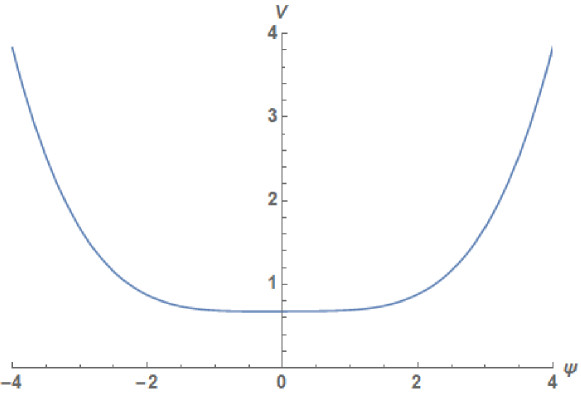
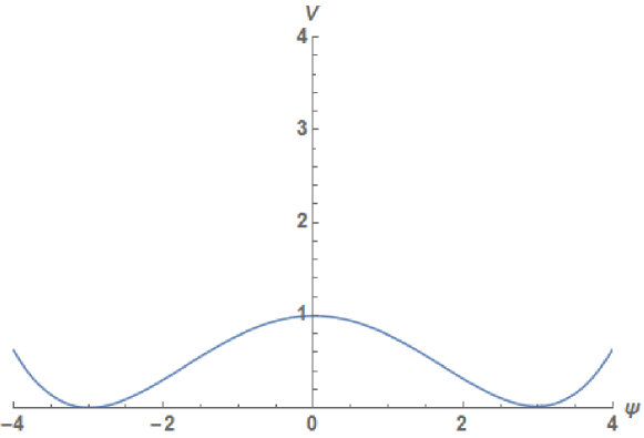
Figure 1: Shape of the potential $V(\psi)$ for constant $\varphi$ at early (top) and late times (bottom), defined relative to the time when $\varphi$ crosses $\varphi_{c}$.

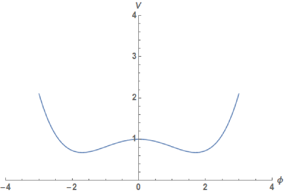
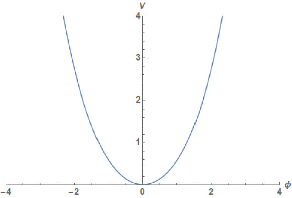
Figure 2: Shape of the potential $V(\varphi)$ for constant $\psi$ at early (top) and late times (bottom), defined relative to the time when $\varphi$ crosses $\varphi_{c}$.

As in the original hybrid model, we start with some $\varphi>\varphi_{c}$ with $\varphi$ quickly rolling down to its minima under an effective $\varphi^{4}$ term. This phase is driven by a simplified potential of the form

$$\frac{V_{\rm eff}^{\varphi}}{M^{4}}=1-\frac{2}{3}\frac{\varphi^{2}}{\varphi_{c}^{2}}+a_{4}\frac{\varphi^{4}}{v^{4}}$$ (30)

since $\psi$ sits in its local minimum at the origin during this time and therefore all $\psi$-terms can be ignored. Once $\varphi$ crosses $\varphi_{c}$, the new true minima of $\psi$ are displaced from the origin due to a tachyonic term in its effective potential, of the form

$$\frac{V_{\rm eff}^{\psi}}{M^{4}}=1+2\left(\frac{\varphi^{2}-\varphi_{c}^{2}}{\varphi_{c}^{2}}\right)\frac{\psi^{2}}{v^{2}}+\frac{4a_{3}\psi}{v^{4}}+\frac{\psi^{4}}{v^{4}}-\frac{2}{3}\frac{\varphi^{2}}{\varphi_{c}^{2}}+a_{4}\frac{\varphi^{4}}{v^{4}}\,,$$ (31)

Due to the $a_{3}$ term, the $Z_{2}$ symmetry of $\psi$ is broken and the field starts slowly rolling away from the origin. This gradual change enables $\varphi$ to closely follow its vacuum expectation value, $\varphi_{*}$. Eventually, $\varphi_{*}$ approaches zero but never reaches it due the uncertainty principle, thereby almost restoring the symmetry for $\varphi$; this is the second phase transition mentioned above. As shown in Figs. 1 and 2, $\varphi$ causes the traditional phase transition when it crosses $\varphi_{c}$, and then the slow roll of $\psi$ down its tachyonic hilltop will end in a second phase transition. The whole process is clarified further by examining how the effective potential changes in time, shown in Figs. 3 and 4.

The hilltop phase generates the dominant number of $e$-folds, and it ends automatically when $\psi$ reaches its new minimum. This is a new feature compared to the traditional hybrid inflation and relies on the existence of a $\varphi^{4}$ term in our effective potential. Our model is not a variant of the original hybrid model [36], such as the inverted-hybrid model [37] or a modified hilltop model [38], or having corrections to the potential coming from supergravity-embedding of the model [39]; rather, we start with a Higgs-like model and include effects from an initial quantum state that turn it into a hybrid model with some additional terms.

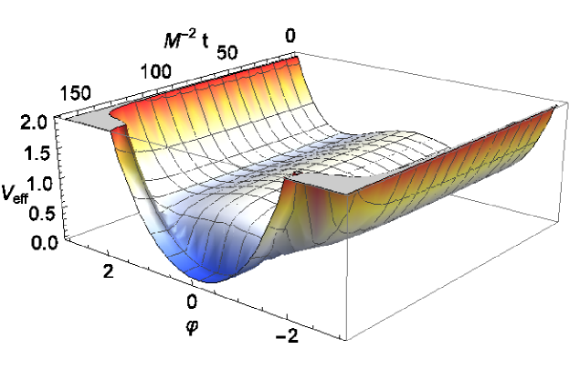
Figure 3: After a brief non-adiabatic phase when it rolls down a steep potential wall, $\varphi$ traces its minimum for the majority of inflation. The growth of $\psi^{2}$ moves the $\varphi$-minima closer to zero, causing another non-adiabatic phase that ends with an approximate symmetry restoration for $\varphi$. The parameters used are $v=3$, $a_{3}=0.05$ and $\delta=0.1$.

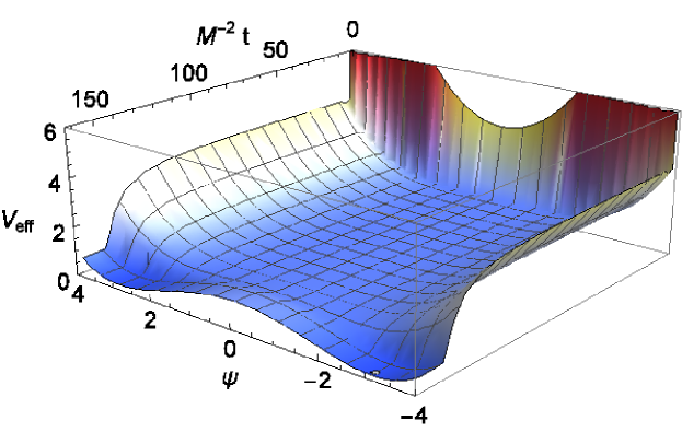
Figure 4: During the initial non-adiabatic phase, a phase transition akin to traditional hybrid models occurs. Reflection symmetry in the potential is slightly broken by the $a_{3}$-term (which is not apparent in the figure due to its smallness). This non-Gaussianity term drives $\psi$ to its new stable point where $\psi^{2}$ approaches $v^{2}$. The parameters are the same as Fig. 3.

3.3 UV-completion and the swampland

One of the conceptual requirements for inflation models is that they should have a well-defined quantum completion. One way to implement this is to derive specific forms of inflationary potentials from string theory constructions as was done, for instance, in the case of natural inflation. Another recent idea has been that of the swampland, a complement of the string landscape, which stems from the fact that not all low-energy effective field theories can be consistently completed in the ultraviolet into a quantum theory of gravity [40, 41]. In order for an effective field theory to be consistent, it would have to satisfy the eponymous swampland constraints. This is a much more general way in which quantum gravity may restrict the form of the potential, amongst other things, in the low-energy effective field theory used as the starting point for inflation. More specifically, it has been argued that many models of (at least) single-field inflation are not consistent with the swampland conjectures since the latter require either a large value for the slope of the potential, $|V^{\prime}|/V>\mathcal{O}(1)$, or large tachyonic directions, $V^{\prime\prime}/V<-\mathcal{O}(1)$ [42].

Taken together, these conjectures severely restrict the lifetime of metastable (quasi-)de Sitter spacetimes that can be built from string theory. In order to obtain an estimate for the numbers of order one that appear in one of them, the so-called de-Sitter conjecture, one has to resort to fundamental properties of quantum gravity such as the absence of eternal inflation [43, 44] or the trans-Planckian censorship conjecture [45, 46]. The latter has put a more concrete bound on the duration of inflation which, when combined with the observed power spectrum, imposes severe constraints on the allowed models for inflation. It has been shown that only hilltop type of models, which generically allow for a small slow-roll parameter $\epsilon$ but a big $\eta$, are the ones that survive amongst all single-field models unless one invokes additional degrees of freedom as in non-Bunch Davies initial states or warm inflation. Even for hilltop potentials, which seem to be the most compatible with the swampland, one has to resort to an arbitrary steepening of the potential to end inflation so as not to have too many $e$-folds since that would once again make the model incompatible with the constraints. To date, there are no string theory realizations of any such single-field potential that can abruptly stop inflation after a finite amount of time.

The remarkable feature of our new model is that it is able to give a viable inflationary cosmology as well as a graceful exit with a tachyonic (p)reheating, all starting from a Higgs-like single-field potential as the main input. We are using only standard quantum mechanics in a non-adiabatic semiclassical approximation and do not have to rely on unknown features of quantum gravity. In addition, by virtue of the fact that the classical field $\psi$ plays the role of the inflaton relevant for observable scales, this model is essentially of the hilltop type which has recently been shown to be preferred by the swampland and to be able to ameliorate the $\eta$-problem [47]. Quantum effects imply that the single-field classical potential is, upon quantization, no longer a single-field model that would have to be tuned in order to avoid having too many $e$-folds of inflation or require any additional mechanism to achieve stability against radiative corrections [48]. Moreover, our detailed derivations below reveal that the model maintains a large value of the slow-roll parameter $\eta$ throughout inflation (in addition to a small $\epsilon$, as is usually the case for a prototype hilltop model). Indeed, it is when the value of $\eta$ becomes too large that inflation ends in this model, once again thanks to effects of quantum fluctuations of the classical field (as opposed to a generic second field). All of this is possible even though we start with a single-field model with a monomial potential, but then take into account the effects of quantum fluctuations in a systematical manner.

4 Analysis

The effective Hamiltonian (2.2) describes a two-field model with standard kinetic terms in an expanding universe and an interaction potential similar to hybrid models. A numerical analysis can be applied directly to Hamilton’s equations for $\psi$ and $\phi$ generated by $H^{\rm closure}_{\rm Q}$, (2.2), using suitable initial values. We will present such solutions in comparison with a slow-roll approximation to be developed first.

4.1 Slow-roll approximation

For inflationary applications of (2.2), we are interested in a long phase of slow roll that can be generated by $\psi$ staying near its initially stable and then metastable equilibrium position at $\psi=0$. As long as $\psi^{2}\ll v^{2}$ and $\varphi^{2}\approx\varphi^{2}_{*}$ is near a local minimum, the slow-roll approximation can be used and evaluated analytically. This phase is adiabatic and therefore does not require all terms in (2.2) that are implied by semiclassical methods for non-adiabatic quantum dynamics. However, as we have already seen, the remaining terms are essential in achieving suitable initial values for the slow-roll phase and to end it early enough. Throughout this analysis, we will also assume small background non-Gaussianity. As our results will show, this assumption is justified by observational constraints on the spectral index.

Given these conditions, the slow-roll parameters can be approximated as

$$\epsilon_{\varphi} \equiv \frac{1}{2}M_{\rm P}^{2}\left(\frac{V_{\varphi}}{V}\right)^{2}\approx\frac{1}{2}M_{\rm P}^{2}\left(\frac{M^{4}}{P}\right)^{2}\left(\frac{4\varphi}{3\varphi_{c}^{2}}\left(1-\frac{3\psi^{2}}{v^{2}}\right)-\frac{4a_{4}\varphi^{3}}{v^{4}}\right)^{2}$$ (32)

$$\epsilon_{\psi} \equiv \frac{1}{2}M_{\rm P}^{2}\left(\frac{V_{\psi}}{V}\right)^{2}\approx\frac{1}{2}M_{\rm P}^{2}\left(\frac{M^{4}}{P}\right)^{2}\left(\frac{4\psi}{v^{2}}\left(\frac{\varphi^{2}}{\varphi_{c}^{2}}+\frac{\psi^{2}}{v^{2}}-1\right)+\frac{4a_{3}}{v^{4}}\right)^{2}$$ (33)

$$\eta_{\varphi\varphi} \equiv M_{\rm P}^{2}\frac{V_{\varphi\varphi}}{V}=-\frac{M^{4}}{P}\left(\frac{4}{3\varphi_{c}^{2}}\left(1-\frac{3\psi^{2}}{v^{2}}\right)-\frac{12a_{4}\varphi^{2}}{v^{2}}\right)$$ (34)

$$\eta_{\psi\psi} \equiv M_{\rm P}^{2}\frac{V_{\psi\psi}}{V}=\frac{M^{4}}{P}\frac{4}{v^{2}}\left(\frac{\varphi^{2}-\varphi^{2}_{c}}{\varphi_{c}^{2}}+\frac{3\psi^{2}}{v^{2}}\right)$$ (35)

$$\eta_{\psi\varphi} \equiv M_{\rm P}^{2}\frac{V_{\varphi\psi}}{V}=\frac{M^{4}}{P}\frac{8\psi\varphi}{v^{2}\varphi_{c}^{2}}\,,$$ (36)

where $V_{\varphi}=\partial V/\partial\varphi$ and $V_{\psi}=\partial V/\partial\psi$, iterated for higher derivatives. The constant $P$ is the initial potential energy, evaluated when $\varphi\approx\varphi_{c}$ and $\psi\approx 0$. In the following we set $M_{\rm P}=1$. We will see later that small non-Gaussianity ensures that $\varphi^{2}/\varphi_{c}^{2}-1\ll 1$. Along with the adiabatic approximation for $\varphi$, this inequality can ensure that $\epsilon_{\psi}$ and $\eta_{\psi\psi}$ are very small. However $\eta_{\varphi\varphi}$ is not necessarily small, even though $\ddot{\varphi}\ll 3H\dot{\varphi}$ and $\dot{\varphi}^{2}\ll V$.

Our equations of motion, under slow roll, then read

$$\frac{3H\dot{\varphi}}{M^{4}} = \frac{4\varphi}{3\varphi_{c}^{2}}\left(1-\frac{3\psi^{2}}{v^{2}}\right)-\frac{4a_{4}\varphi^{3}}{v^{4}}$$ (37)

$$\frac{3H\dot{\psi}}{M^{4}} = -\frac{4\psi}{v^{2}}\left(\frac{\varphi^{2}-\varphi_{c}^{2}}{\varphi_{c}^{2}}+\frac{\psi^{2}}{v^{2}}\right)-\frac{4a_{3}}{v^{4}}\,.$$ (38)

where we can make $M$ implicit by rescaling $t\rightarrow t/M^{2}$. The regime covered by our approximations can be split into two phases followed by an end phase.

4.1.1 Phase 1

In early stages, we have $\psi^{2}\ll v^{2}$ and can thus ignore the term $3\psi^{2}/v^{2}$ in (37). Therefore, the constant $\varphi^{2}\approx\varphi^{2}_{*}\approx 3\varphi^{2}_{c}/a_{4}$ is a solution. Adiabaticity ensures that we can expand the equation of motion around the critical point $\varphi_{*}$ where $V_{\varphi}(\varphi_{*})=0$:

$$\dot{\varphi}\approx-\frac{1}{3H}V_{\varphi\varphi}(\varphi_{*})(\varphi-\varphi_{*})\,.$$ (39)

Defining $\varphi^{\prime}:={\rm d}\varphi/{\rm d}N$ where $N$ is the number of $e$-folds, we obtain

$$\varphi^{\prime}\approx-\eta_{\varphi\varphi}(\varphi=\varphi_{*},\psi\approx 0)(\varphi-\varphi_{*})\,.$$ (40)

For small non-Gaussianity, we have $a_{4}=3+\delta$ with $\delta\ll 1$. Choosing the initial value $\varphi(0)=\varphi_{c}$ for Phase 1 therefore implies

$$\varphi_{1}(N)\approx\frac{\varphi_{c}\delta}{2a_{4}}\exp(-\eta_{\varphi\varphi}(\varphi_{*},0)N)+\varphi_{*}\,.$$ (41)

Note that small non-Gaussianity also implies $\varphi_{*}^{2}=\varphi_{c}^{2}+O(\delta)+O(\psi^{2})$.

We can expect $\varphi^{2}/\varphi_{c}^{2}-1\approx-\delta/a_{4}$ to be much bigger than $\psi^{2}/v^{2}$ at early times. This reduces the second equation of motion, (38), to

$$\psi^{\prime}\approx\frac{1}{P}\frac{4}{v^{2}}\left(\frac{\delta}{a_{4}}\psi-\frac{a_{3}}{v^{2}}\right)$$ (42)

which is solved by

$$\psi_{1}(N)\approx-\frac{a_{3}a_{4}}{\delta v^{2}}\left(\exp\left(\frac{4\delta}{v^{2}a_{4}P}N\right)-1\right)$$ (43)

for an initial $\psi_{1}$ at the origin. To summarize, Phase 1 is characterized mathematically by the possibility to ignore the $\psi^{2}/v^{2}$ terms in (37) and (38).

4.1.2 Phase 2

As $\psi$ moves away from its metastable position at $\psi=0$, the terms $\psi^{2}/v^{2}$ in the equations of motion will eventually have noticeable effects even while they may still be small. In particular, the local minimum of $\varphi$ at

$$\varphi_{*}(\psi(t))^{2}=\frac{v^{4}}{3\varphi_{c}^{2}a_{4}}\left(1-\frac{3\psi(t)^{2}}{v^{2}}\right)$$ (44)

is then time-dependent. The solution for $\varphi$ in Phase 2 can therefore be obtained directly from (41) by inserting the time-dependent $\psi$ and $\varphi_{*}$,

$$\varphi_{2}(N)=\varphi_{1}(N)|_{\psi\rightarrow\psi(N)}\,,$$ (45)

using the solution for $\psi(N)\equiv\psi_{2}(N)$ to be derived now. As implied by adiabaticity, we still have $\varphi^{2}\approx\varphi_{*}^{2}$, tracking the local minimum.

Our phase now is described by the first two terms of (38) dominating over the $a_{3}$-term. Therefore,

$$\psi^{\prime} \approx -\frac{1}{P}\frac{4\psi}{v^{2}}\left(\frac{\varphi_{*}(\psi(t))^{2}-\varphi_{c}^{2}}{\varphi_{c}^{2}}+\frac{\psi^{2}}{v^{2}}\right)$$ (46)

$$= \frac{1}{P}\frac{4\psi}{v^{2}}\left(\frac{\delta}{a_{4}}+\frac{2\psi^{2}}{v^{2}}+O(\delta\psi^{2}/v^{2})\right)\,.$$

which is solved by

$$\psi_{2}(N)\approx-\operatorname{sgn}(a_{3})\sqrt{\frac{\delta}{(2a_{4}/v^{2}+\delta/\psi_{\rm g}^{2})\exp(-8\delta(N-N_{\rm g})/(v^{2}Pa_{4}))-2a_{4}/v^{2}}}\,.$$ (47)

(Although $a_{3}$ does not appear in our approximate equation (46), its sign determines the direction in which $\psi$ starts moving as a consequence of reflection symmetry breaking.) Here, the subscript “g” denotes the value of solutions at the “gluing” point of the two phases, defined as the point where the cubic term in (38) is on the order of the $a_{3}$-term; see Fig. 6 below for an illustration.

4.1.3 End phase

Even though Phase 1 and Phase 2 are sufficient to describe the majority of inflation, finding the point at which inflation ends requires a qualitatively different approximation compared with the above two phases. The physics is also quite different. To see this, note that if we extend the approximations of Phase 2 too far, we arrive at two wrong conclusions. First, $\psi$ will eventually cross the point $\psi^{2}=v^{2}/3$, such that the two minima of $V_{\rm eff}(\varphi)$ meet at $\varphi_{*}=0$. Second, this behavior causes $\varphi$ to approach zero, such that the field $\psi$ ends up at its new $V_{\rm eff}(\psi)$-minimum, $\psi_{\rm min}=-v$ (assuming $a_{3}$ is positive). The former ($\varphi\to 0$) is forbidden by the uncertainty principle, embodied in our $U$-term in $V_{\rm eff}$ neglected so far in the slow-roll analysis, and the latter is erroneous since it implies that once everything has settled, $H^{2}$, which is proportional to $V_{\rm eff}$ during slow roll, would seem to approach a negative value $4a_{3}\psi/v^{4}<0$.

However, this last conclusion certainly cannot be correct because our classical potential (1), a complete square $V_{\rm cl}(\psi)=M^{4}(1-\psi^{2}/v^{2})^{2}$, is positive semidefinite. Therefore, it is quantized to a positive, self-adjoint operator $\hat{V}$ which cannot possibly have a negative expectation value $V_{\rm eff}=\langle\hat{V}\rangle$ in any admissible state. In terms of moments used in our canonical effective description, after $\psi$ crosses the value $v^{2}/3$, the fluctuation variable $\varphi$ shrinks. Therefore, according to our moment closure introduced after equation (17), the variance $\Delta(\psi^{2})=\varphi^{2}$ as well as the fourth-order moment $\Delta(\psi^{4})=a_{4}\varphi^{4}$ approach zero, while $\Delta(\psi^{3})=a^{3}$ has so far been assumed constant. This latter assumption violates higher-order uncertainty relations for small $\varphi$.

We will not require a precise form of such higher-order uncertainty relations, or a specific decreasing behavior of $\Delta(\psi^{3})$ because, referring to positivity, we know that the magnitude of the $a_{3}$-term in the potential is not allowed to be larger than the sum of the rest of the terms in $V_{\rm eff}$. (But see the next subsection for numerical examples with decreasing $\Delta(\psi^{3})$.) This observation places an implicit bound on non-Gaussianity parameters when our potential energy decreases at the end of inflation. Taking this outcome into account, our effective potential eventually becomes

$$\frac{V_{\rm eff}}{M^{4}}\approx\left(1-\frac{\psi^{2}}{v^{2}}\right)^{2}+\frac{2}{3}\frac{\varphi^{2}}{\varphi_{c}^{2}}\left(\frac{3\psi^{2}}{v^{2}}-1\right)+\frac{U}{2M^{4}a^{6}V_{0}^{2}\varphi^{2}}\,,$$ (48)

where we have neglected the $\varphi^{4}$ and $a_{3}$ terms for small fluctuations. The corrected values $\varphi_{*}$ of the two $\varphi$-minima are now

$$\varphi_{*}\approx\pm\left(\frac{u}{K(\psi^{2})}\varphi_{c}^{2}\right)^{1/4}$$ (49)

where

$$u=\frac{U}{M^{4}a^{6}V_{0}^{2}}\quad\mbox{and}\quad K(\psi^{2})=\frac{4}{3}\left(\frac{3\psi^{2}}{v^{2}}-1\right)\,.$$ (50)

Since $u$ is extremely small after $60$ $e$-folds, we have $|\varphi_{*}|\ll 1$. The symmetry restoration for $\varphi$ is therefore only an approximate one. In addition, we neglected the $O(\delta\psi^{2}/v^{2})$-term in (46), but kept $\delta/a_{3}$. These two terms become comparable around $\psi^{2}=v^{2}/3$ for our chosen parameters. However, as we will see later in a comparison with numerical solutions, setting $\varphi=0$ and using the $\psi(N)$ expression of Phase 2 during the end phase gives a sufficiently accurate number of $e$-folds.

4.2 Comparison of analytical and numerical solutions

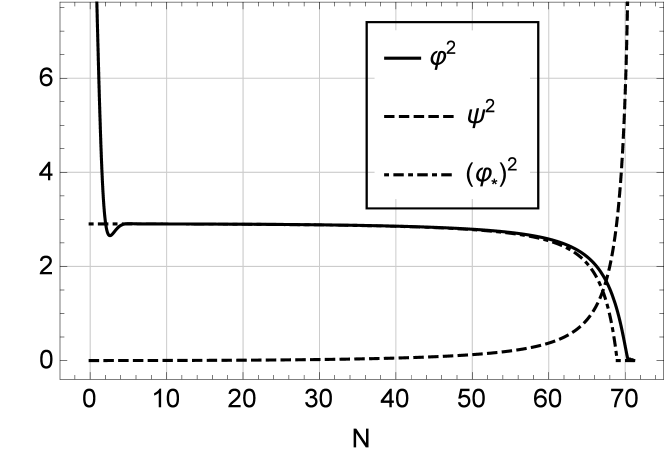
Figure 5: Overview of full numerical evolution. The field $\psi$ remains small during inflation while $\varphi$ follows its vacuum expectation value $\varphi_{*}$ very closely throughout the whole evolution. After inflation ends, $\psi^{2}$ approaches $v^{2}$, a value cut off in this presentation. While the fields may take Planckian values, of the order one in natural units, except for very early times they hover near their potential minima where they imply sub-Planckian energy densities. Quantum-gravity effects are therefore negligible during inflation. The field $\psi^{2}$ increases at the end of inflation, but it merely approaches its new minimum seen in Fig. 4 and is not a run-away solution.

Our analytical solutions were obtained with certain approximations, but they generally agree well with numerical solutions of the full equations,

$$\ddot{\varphi}+3H\dot{\varphi} = \frac{4\varphi}{3\varphi_{c}^{2}}\left(1-\frac{3\psi^{2}}{v^{2}}\right)-\frac{4a_{4}\varphi^{3}}{v^{4}}$$ (51)

$$\ddot{\psi}+3H\dot{\psi} = -\frac{4\psi}{v^{2}}\left(\frac{\varphi^{2}-\varphi_{c}^{2}}{\varphi_{c}^{2}}+\frac{\psi^{2}}{v^{2}}\right)-\frac{4a_{3}}{v^{4}}\,,$$ (52)

in situations relevant for inflation. To be specific, we choose parameters $v=3$, $\delta=0.1$ and $a_{3}=0.05$ in our numerical solutions. Figure 5 shows a representative example of full numerical evolution. To test our analytical assumptions, Fig. 6 shows the magnitudes of individual terms that contribute to the equation of motion (52) for $\psi$, while Figs. 7 and 8 compare analytical and numerical solutions of both equations.

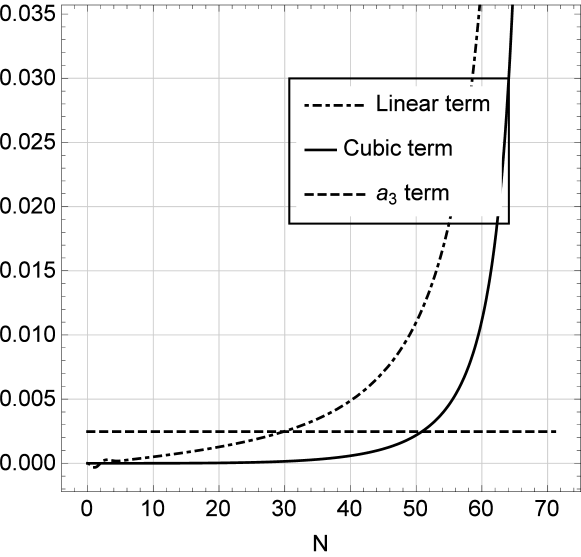
Figure 6: The magnitudes of individual terms in (38) as functions of $N$. The term $\psi^{3}/v^{4}$ in (38) approaches the order of $a_{3}/v^{4}$ around $N=50$, marking the transition point to Phase 2.

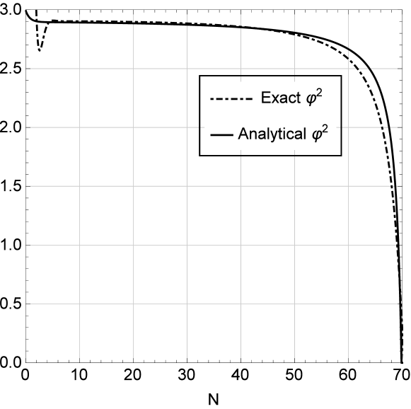
Figure 7: Comparison of analytical and numerical solutions for $\varphi(N)$. Our analytical solution for $\varphi(N)$ agrees well with the full numerical one, justifying the adiabatic approximation during inflation.

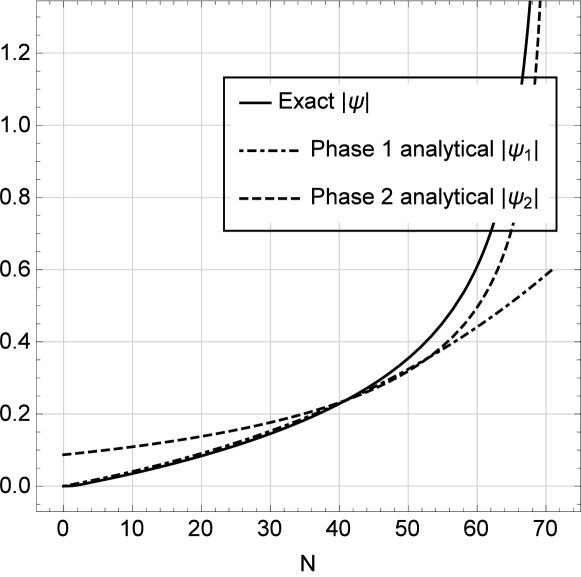
Figure 8: Comparison of analytical and numerical solutions for $\psi(N)$. The analytical solution agrees extremely well with the exact one in Phase 1 (before $N=50$), while small deviations occur in $\psi_{2}$ occur Phase 2 (after about $N=50$).

Cosmological parameters relevant for inflation are shown in the next figures, Fig. 9 for the slow-roll parameter $\eta_{\psi\psi}$ which eventually ends inflation, Fig. 10 for the spectral index according to both analytical and numerical solutions, as well as its running in Fig. 11. As shown by these figures, the paramaters easily imply solutions compatible with observational constraints. It is also shown how $\eta_{\psi\psi}$ increases at an opportune time to end inflation with just the right number of $e$-folds in order to avoid the trans-Planckian problem.

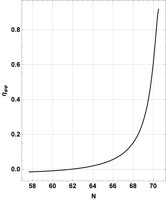
Figure 9: Late time behavior (Phase 2) of $\eta_{\psi\psi}(N)$ obtained from analytical solutions for $\psi(N)$ and $\varphi(N)$. The slow-roll assumption starts being violated around $N\sim 70$, effectively ending inflation.

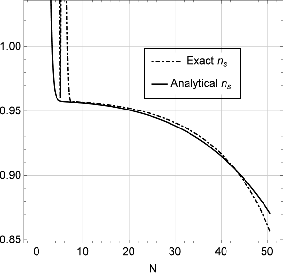
Figure 10: Analytical and numerical solutions for the spectral index $n_{\rm s}(N)$ in Phase 1. Since Hubble exit takes place at least a $\Delta N\sim 60$ prior to the end of inflation, it can only occur in Phase 1. Importantly, $n_{\rm s}\approx 0.96$ at $\Delta N\sim 60$.

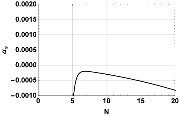
Figure 11: Analytical solution for the running $\alpha_{\rm s}\approx{\rm d}n_{\rm s}/{\rm d}N$ [49] at early times, using a non-Gaussianity parameter $a_{3}=0.05$. Estimating Hubble exit at $N\sim 10$, $\alpha_{\rm s}$ is well within Planck’s upper bound on the magnitude ($\sim 10^{-3}$).

The role of non-Gaussianity parameters can also be studied. For instance, parameterizing $a_{3}=0.01\varphi^{3}$ instead of a constant $a_{3}=0.05$ leads to comparable results, as shown for the number of $e$-folds in Fig. 12. The effects of different choices of $\delta=a_{4}-3$ on the spectral index and the tensor-to-scalar ratio (computed as $r\approx 16\epsilon_{\sigma}$, $\sigma$ being the effective adiabatic field [34]) are shown in Figs. 13 and 14. An important new result is that the non-Gaussianity parameters effectively control the onset and duration of inflation, such that observationally preferred numbers of $e$-folds can be obtained for reasonable choices of background non-Gaussianity. In particular, only small deviations from a nearly Gaussian ground state are required.

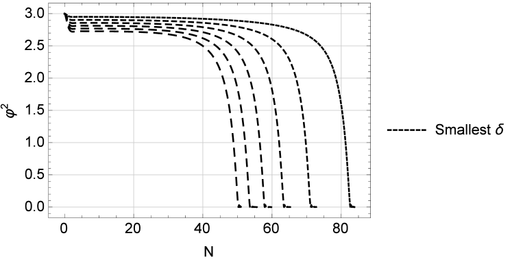
Figure 12: Evolution of $\varphi(N)^{2}$, from numerical solutions using $a_{3}=0.01\varphi^{3}$. Inflation ends at $N_{e}$ where $\varphi(N_{e})\approx 0$. Different curves correspond to different values of $a_{4}$, or $\delta=a_{4}-3$, where $\delta=0.05,0.1,0.15,0.2,0.25,3$. Smaller $\delta$ increase the duration of inflation.

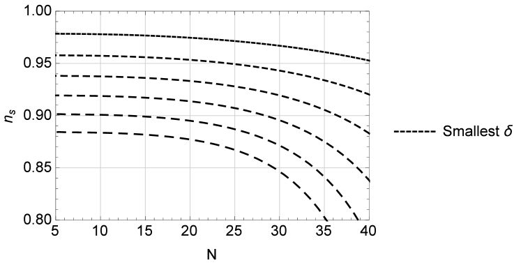
Figure 13: Spectral index $n_{\rm s}(N)$ as a function of $e$-folds $N$ at Hubble exit from numerical solutions, using $a_{3}=0.01\varphi^{3}$. Different curves correspond to different values of $a_{4}$, or $\delta=a_{4}-3$, where $\delta=0.05,0.1,0.15,0.2,0.25,3$. Smaller $\delta$ brings the spectral index closer to one.

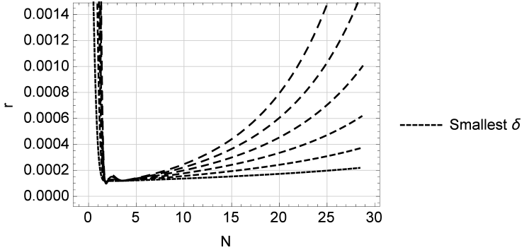
Figure 14: Tensor-to-scalar ratio $r(N)$ as a function of $e$-folds at Hubble exit from numerical solutions, using $a_{3}=0.01\varphi^{3}$. Different curves correspond to different values of $a_{4}$, or $\delta=a_{4}-3$, where $\delta=0.05,0.1,0.15,0.2,0.25,3$. Smaller $\delta$ decrease $r$.

4.3 Analytical results for cosmological observables

Now we use the approximate analytical solutions to predict the number of $e$-folds $N$ (starting from the crossing of $\phi=\phi_{c}$) and the spectral index. In our model, both the classical field and its quantum fluctuation undergo slow-roll evolution in different phases of the dynamics. Therefore, they should both contribute to the curvature perturbation and one can write down the effective adiabatic field $\sigma$ as a combination of both these fields, $\psi$ and $\phi$.

In terms of the adiabatic field, consider the spectral index at around horizon exit,

$$n_{s}=1-6\epsilon_{\sigma}+2\eta_{\sigma\sigma}\,.$$ (53)

At early times, using the adiabatic approximation for $\phi$ and small $\psi$, we have

$$\epsilon_{\sigma}=\epsilon_{\psi}+\epsilon_{\varphi}\approx 0+O(\psi^{2},\delta^{2},a_{3}^{2})\,.$$ (54)

For $\eta_{\sigma\sigma}$ we have [34]

$$\eta_{\sigma\sigma} = \eta_{\varphi\varphi}\cos^{2}\theta+\eta_{\psi\psi}\sin^{2}\theta+2\eta_{\varphi\psi}\sin\theta\cos\theta$$ (55)

where $\theta$ is defined such that

$$\cos\theta=\frac{\dot{\varphi}}{\sqrt{\dot{\varphi}^{2}+\dot{\psi}^{2}}}\quad,\quad\sin\theta=\frac{\dot{\psi}}{\sqrt{\dot{\varphi}^{2}+\dot{\psi}^{2}}}\,.$$ (56)

Using the slow roll equations of motion for $\psi$ and $\dot{\varphi}\approx\dot{\varphi}_{*}=-3\psi(a_{4}\varphi_{*})^{-1}\dot{\psi}$ we obtain

$$\cos\theta\approx-\frac{3\psi}{a_{4}\varphi_{*}}\sin\theta\quad,\quad\sin\theta\approx 1\,,$$ (57)

where we used $V_{\psi}\gg V_{\varphi}\approx 0$. To leading order of $\psi$, we therefore have

$$\eta_{\varphi\varphi}\cos^{2}\theta \approx 0+O(\delta^{2},\alpha_{3}^{2},\psi^{2})$$ (58)

$$\eta_{\varphi\psi}\sin\theta\cos\theta \approx 0+O(\psi^{2})$$ (59)

$$\eta_{\psi\psi}\sin^{2}\theta \approx -\frac{4\delta}{a_{4}Pv^{2}}+O(\psi^{2})\,,$$ (60)

such that

$$n_{\rm s}\approx 1-\frac{8\delta}{a_{4}Pv^{2}}\,.$$ (61)

Evaluating

$$P\equiv V(\varphi_{*}(\psi=0),\psi=0)=1-\frac{1}{a_{4}}\approx\frac{2}{3}+\frac{\delta}{9}+O(\delta^{2})$$ (62)

leads to the final expression

$$n_{\rm s}\approx 1-12\frac{\delta}{a_{4}v^{2}}+O(\delta^{2})\,.$$ (63)

Imposing a slow-roll condition such as $\eta_{\psi\psi}\sim 10^{-2}$ requires $v^{2}/\delta\sim O(10^{2})$, which implies typical values of $n_{\rm s}$ in the range $0.9<n_{\rm s}<1$.

Now, for total number of $e$-folds $N_{e}$ we first need to find the value $\psi_{e}$ of $\psi$ at which inflation ends. Approximately, this stage occurs when

$$\eta_{\psi\psi}(\varphi_{*},\psi_{e})=\frac{V_{\psi\psi}}{V}|_{\varphi=\varphi_{*},\psi=\psi_{e}}\approx 1$$ (64)

during the end phase. Under the approximation $\varphi\approx 0$, we have

$$\frac{V_{\psi\psi}}{V}\approx\frac{4}{v^{2}}\frac{3\psi^{2}/v^{2}-1}{(1-\psi^{2}/v^{2})^{2}}\,.$$ (65)

Then $V_{\psi\psi}\approx V(\varphi_{*},\psi)$ gives

$$\frac{\psi_{e}^{2}}{v^{2}} \approx 1+\frac{6}{v^{2}}\pm 2\sqrt{\frac{9}{v^{4}}+\frac{2}{v^{2}}}$$ (66)

$$= 1+\frac{6}{v^{2}}\left(1-\sqrt{1+\frac{2v^{2}}{9}}\right)\,,$$ (67)

where we chose the minus sign in the second line. From the above expression we see that typically $\psi_{e}^{2}/v^{2}-1/3\sim O(10^{-1})$. Then using

$$\Delta\psi\sim-\frac{V_{\psi}}{V}\Delta N\sim O(1)\Delta N\,,$$ (68)

we see that that beyond $\psi^{2}/v^{2}=1/3$, we do not get many $e$-folds before reaching the point $\eta_{\psi\psi}\approx 1$, effectively ending inflation. In terms of the total number of $e$-folds, it is therefore justified to approximate

$$\psi_{2}(N)^{2}\approx v^{2}/3\quad\mbox{such that}\quad\varphi_{*}^{2}=0$$ (69)

as the end point of inflation.

Since our analytical solution consists of $\psi_{1}$ and $\psi_{2}$, to find the total number of $e$-folds $N_{e}$ at $\psi_{2}^{2}=v^{2}/3$, we must first find the number of $e$-folds $N_{\rm g}$ at the gluing point. By definition of the latter,

$$\psi_{\rm g}^{3}\equiv\psi_{1}(N_{\rm g})^{3}=-a_{3}\,.$$ (70)

Denoting

$$\eta\equiv|\eta_{\psi\psi}(\varphi_{1},\psi_{1})|\approx\frac{4\delta}{a_{4}Pv^{2}}\approx\frac{6\delta}{a_{4}v^{2}}+O(\delta^{2})\,,$$ (71)

we have

$$2\eta=1-n_{\rm s}\,.$$ (72)

Using (43),

$$\exp(\eta N_{\rm g})=\frac{v^{2}}{\psi_{\rm g}^{2}}\frac{\delta}{a_{4}}+1$$ (73)

which, inserted in (47), using (72) and setting $\psi_{2}(N_{e})^{2}=v^{2}/3$, implies

$$N_{e}=\frac{1}{1-n_{\rm s}}\left(\log\left(\frac{2}{v^{2}}+\frac{1-n_{\rm s}}{12}\chi\right)+2\log\left(\frac{1-n_{\rm s}}{12}\chi v^{2}+1\right)-\log\left(\frac{2}{v^{2}}+\frac{1-n_{s}}{4}\right)\right)\,,$$ (74)

where $\chi\equiv v^{2}/\psi_{g}^{2}$. The relationship (74) is illustrated in Fig. 15.

Aside from the parameter $v$ that appears in common Higgs-like or hybrid models, our observables depend on two new parameters $a_{3}$ and $\delta$ which describe the non-Gaussianity of the background state. Background non-Gaussianity effectively controls the amount of non-adiabatic evolution due to its modulation on the shifting of local $\varphi$-minima at $\varphi_{*}$. The dependence of the number of $e$-folds on the non-Gaussianity parameter $a_{3}$ is shown in Fig. 16, using the analytical solutions.

The dependence (74) of $N_{e}$ on $n_{\rm s}$ is more complicated than in non-minimal Higgs models, but it is nevertheless related. To facilitate a comparison, we rewrite the expression as

$$N_{e}\approx\frac{f(1-n_{\rm s},v,a_{3})}{1-n_{\rm s}}$$ (75)

where the function $f$ describes a weak, logarithmic dependence on $1-n_{\rm s}$. In non-minimal Higgs inflation, the analog of the function $f(1-n_{\rm s},v,\alpha_{3})$ is constant ($f=2$) [6]. Here, the function increases logarithmically with growing $1-n_{\rm s}$, taking values in the range $1\lesssim f(1-n_{\rm s},v,a_{3})\lesssim 5$ for typical parameter values considered in our analysis. (An abbreviated derivation of (75) can be found in [10].)

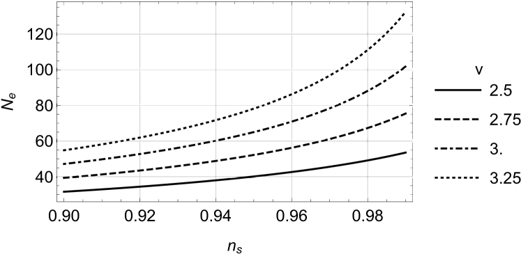
Figure 15: The number of $e$-folds, $N_{e}$, increases as a function of the spectral index $n_{\rm s}$, using the approximate relation (74). The function is shown for varying parameters $v$ in the potential, while $a_{3}=0.05$. As a function of the non-Gaussianity parameters, the number of $e$-folds decreases; see Fig. 16. (Note that in the analytical relation (63), the variation of $n_{\rm s}$ mirrors the non-Gaussianity ratio $\delta/(a_{4}v^{2})$.)

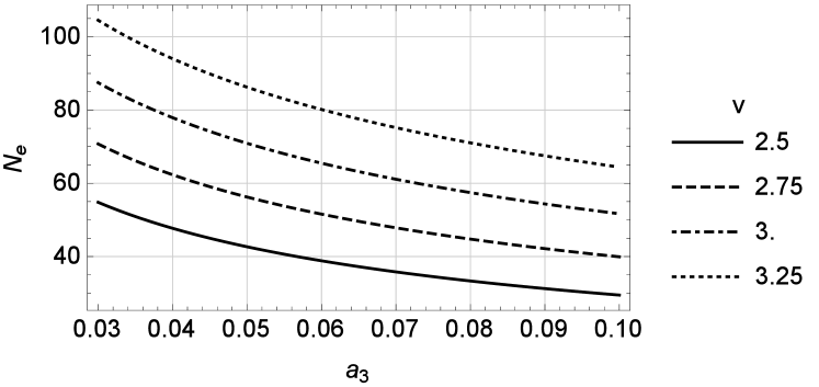
Figure 16: The number of $e$-folds, $N_{e}$, decreases with the amount of non-Gaussianity, parameterized by $a_{3}$, shown here for fixed $n_{\rm s}\approx 0.96$, $\delta=0.1$ and using (74). Background non-Gaussianities increases the departure from adiabatic evolution, effectively ending inflation earlier than desired.

5 Conclusions

Typically, potentials for the inflaton field are postulated so as to match existing observations. On the other hand, one of the most remarkable successes of inflation is that it explains the large-scale structure of the universe as originating from quantum vacuum fluctuations. It is inconceivable to quantize the fluctuations of the inflaton field alone without taking into account the quantum corrections to the background field potential. In other words, one cannot simply express the inflationary potential in terms of expectation values of the homogeneous background field, but should also take fluctuations and higher moments of the quantum state into account. It is customary to express the resulting effective potential in a derivative expansion (of the Coleman-Weinberg type); however, this method is not sufficient if one has to consider non-adiabatic evolution of the inflaton field. Although a slow-rolling field does seem to justify an adiabatic approximation, in this work we have shown how non-adiabaticity can play a crucial role setting up the initial conditions for a slow roll phase as well as help in ending it. We have presented a more general procedure for calculating the effects of such non-adiabatic evolution in the context of early-universe cosmology.

We have presented an observationally consistent extension of Higgs-like inflation by introducing non-adiabatic quantum effects in a semiclassical approximation although our formalism is applicable more generally for any inflationary potential. As shown, these effects imply that the classical potential is not only corrected in its coefficients but is also amended by new terms for independent quantum degrees of freedom, in particular the quantum fluctuation of the Higgs field. The original single-field model is therefore turned into a multi-field model. The multi-field terms incorporate quantum corrections of the background field, corresponding to backreaction of radiative corrections. Since the single-field potential is renormalizable, our quantum scenario is robust from the perspective of quantum field theory.

New interaction terms in the multi-field potential have coupling constants that depend on the background state, parameterizing its non-Gaussianity. They imply two new non-adiabatic phases that cannot be seen in low-energy potentials or in cosmological studies based completely on slow-roll approximations. In particular, an initial non-adiabatic phase, combined with the uncertainty relation for the fluctuation degree of freedom, sets successful initial conditions for inflation to take place, and a second non-adiabatic phase ends inflation after the right number of $e$-folds. Observational constraints show that background non-Gaussianity should be small, but it must be non-zero for the non-adiabatic phases to be realized. Our model is highly constrained because non-Gaussianity is bounded from below, but we are nevertheless able to derive successful inflation in the range of parameters available to us.

Our model presents a new picture on the role of the quantum state in inflationary cosmology. Quantum fluctuations do not only provide the seeds of structure as initial conditions for perturbative inhomogeneity, they also play a crucial role in guiding the inflationary dynamics of the background state. With further analysis and observations, it may be possible to further constrain the quantum state of the inflaton based on cosmological investigations.

References

- [1] P. A. R. Ade and others [Planck Collaboration], Planck 2013 results. XXII. Constraints on inflation, Astron. Astrophys. 571 (2014) A22, [arXiv:1303.5082]
- [2] A. A. Starobinsky, A new type of isotropic cosmological models without singularity, Phys. Lett. B 91 (1980) 99–102
- [3] G. Isidori, V. S. Rychkov, A. Strumia and N. Tetradis, Gravitational corrections to standard model vacuum decay, Phys. Rev. D 77 (2008), 025034, [arXiv:0712.0242]
- [4] M. Fairbairn, P. Grothaus and R. Hogan, The Problem with False Vacuum Higgs Inflation, JCAP 06 (2014) 039, [arXiv:1403.7483]
- [5] Y. Hamada, H. Kawai and K. y. Oda, Minimal Higgs inflation, PTEP 2014 (2014) 023B02, [arXiv:1308.6651]
- [6] F. L. Bezrukov and M. E. Shaposhnikov, The Standard Model Higgs boson as the inflaton, Phys. Lett. B 659 (2008) 703–706, [arXiv:0710.3755]
- [7] C. Steinwachs, Higgs field in cosmology, In S. De Bianchi and C. Kiefer, editors, 100 Years of Gauge Theory. Past, present and future perspectives. Springer International Publishing, 2020, [arXiv:1909.10528]
- [8] F. Bezrukov and M. Shaposhnikov, Standard Model Higgs boson mass from inflation: Two loop analysis, JHEP 07 (2009) 089, [arXiv:0904.1537]
- [9] C. P. Burgess, H. M. Lee and M. Trott, Comment on Higgs Inflation and Naturalness, JHEP 07 (2010) 007, [arXiv:1002.2730]
- [10] M. Bojowald, S. Brahma, S. Crowe, D. Ding, and J. McCracken, Quantum Higgs Inflation, arXiv:2011.02355
- [11] R. Jackiw and A. Kerman, Time Dependent Variational Principle And The Effective Action, Phys. Lett. A 71 (1979) 158–162
- [12] F. Arickx, J. Broeckhove, W. Coene, and P. van Leuven, Gaussian Wave-packet Dynamics, Int. J. Quant. Chem.: Quant. Chem. Symp. 20 (1986) 471–481
- [13] R. A. Jalabert and H. M. Pastawski, Environment-independent decoherence rate in classically chaotic systems, Phys. Rev. Lett. 86 (2001) 2490–2493
- [14] O. Prezhdo, Quantized Hamiltonian Dynamics, Theor. Chem. Acc. 116 (2006) 206
- [15] T. Vachaspati and G. Zahariade, A Classical-Quantum Correspondence and Backreaction, Phys. Rev. D 98 (2018) 065002, [arXiv:1806.05196]
- [16] M. Mukhopadhyay and T. Vachaspati, Rolling with quantum fields, [arXiv:1907.03762]
- [17] B. Baytaş, M. Bojowald, and S. Crowe, Faithful realizations of semiclassical truncations, Ann, Phys. 420 (2020) 168247, [arXiv:1810.12127]
- [18] B. Baytaş, M. Bojowald, and S. Crowe, Effective potentials from canonical realizations of semiclassical truncations, Phys. Rev. A 99 (2019) 042114, [arXiv:1811.00505]
- [19] M. Bojowald and A. Skirzewski, Effective Equations of Motion for Quantum Systems, Rev. Math. Phys. 18 (2006) 713–745, [math-ph/0511043]
- [20] M. Bojowald and A. Skirzewski, Quantum Gravity and Higher Curvature Actions, Int. J. Geom. Meth. Mod. Phys. 4 (2007) 25–52, [hep-th/0606232], Proceedings of “Current Mathematical Topics in Gravitation and Cosmology” (42nd Karpacz Winter School of Theoretical Physics), Ed. Borowiec, A. and Francaviglia, M.
- [21] M. Bojowald, D. Brizuela, H. H. Hernandez, M. J. Koop, and H. A. Morales-Técotl, High-order quantum back-reaction and quantum cosmology with a positive cosmological constant, Phys. Rev. D 84 (2011) 043514, [arXiv:1011.3022]
- [22] V. I. Arnold, Mathematical Methods of Classical Mechanics, Springer, 1997
- [23] A. Cannas da Silva and A. Weinstein, Geometric models for noncommutative algebras, volume 10 of Berkeley Mathematics Lectures, Am. Math. Soc., Providence, 1999
- [24] O. Prezhdo and Yu.Ṽ. Pereverzev, Quantized Hamilton Dynamics, J. Chem. Phys. 113 (2000) 6557
- [25] C. Kühn, Moment Closure—A Brief Review, In Control of Self Organizing Non-Linear Systems, pages 253–271, Springer International Publishing, 2016
- [26] M. Bojowald and S. Brahma, Minisuperspace models as infrared contributions, Phys. Rev. D 92 (2015) 065002, [arXiv:1509.00640]
- [27] M. Bojowald, The BKL scenario, infrared renormalization, and quantum cosmology, JCAP 01 (2019) 026, [arXiv:1810.00238]
- [28] S. Coleman and E. Weinberg, Radiative corrections as the origin of spontaneous symmetry breaking, Phys. Rev. D 7 (1973) 1888–1910
- [29] M. Bojowald and S. Brahma, Canonical derivation of effective potentials (2014), [arXiv:1411.3636]
- [30] A. D. Linde, Hybrid inflation, Phys. Rev. D 49 (1994) 748–754
- [31] J. Martin and R. H. Brandenberger, The Trans-Planckian Problem of Inflationary Cosmology, Phys. Rev. D 63 (2001) 123501, [hep-th/0005209]
- [32] R. H. Brandenberger and J. Martin, The Robustness of Inflation to Changes in Super-Planck-Scale Physics, Mod. Phys. Lett. A 16 (2001) 999–1006, [astro-ph/0005432]
- [33] J. C. Niemeyer, Inflation with a Planck-scale frequency cutoff, Phys. Rev. D 63 (2001) 123502, [astro-ph/0005533]
- [34] H. Kodama, K. Kohri, and K. Nakayama, On the waterfall behavior in hybrid inflation, Prog. Theor. Phys. 126 (2011) 331–350, [arXiv:1102.5612]
- [35] S. Clesse, Hybrid inflation along waterfall trajectories, Phys. Rev. D 83 (2011) 063518, [arXiv:1006.4522]
- [36] E. D. Stewart, Mutated hybrid inflation Phys. Lett. B 345 (1995) 414-415, [arXiv:astro-ph/9407040]
- [37] D. H. Lyth and E. D. Stewart, More varieties of hybrid inflation Phys. Rev. D 54 (1996) 7186-7190, [arXiv:hep-ph/9606412]
- [38] K. Kohri, C. M. Lin and D. H. Lyth, More hilltop inflation models JCAP 12 (2007) 004, [arXiv:0707.3826]
- [39] R. Jeannerot and M. Postma, Confronting hybrid inflation in supergravity with CMB data JHEP 05 (2005) 071, [arXiv:hep-ph/0503146]
- [40] C. Vafa, The String Landscape and the Swampland, [hep-th/0509212]
- [41] E. Palti, The Swampland: Introduction and Review, Fortsch. Phys. 67 (2019) 1900037, [arXiv:1903.06239]
- [42] H. Ooguri, E. Palti, G. Shiu and C. Vafa, Distance and de Sitter Conjectures on the Swampland Phys. Lett. B 788 (2019) 180-184, [arXiv:1810.05506]
- [43] S. Brahma and S. Shandera, Stochastic eternal inflation is in the swampland, JHEP 11 (2019) 016, [arXiv:1904.10979]
- [44] T. Rudelius, Conditions for (No) Eternal Inflation, JCAP 08 (2019) 009, [arXiv:1905.05198]
- [45] A. Bedroya and C. Vafa, Trans-Planckian Censorship and the Swampland, [arXiv:1909.11063]
- [46] A. Bedroya, R. H. Brandenberger, M. Loverde, and C. Vafa, Trans-Planckian Censorship and Inflationary Cosmology, Phys. Rev. D 101 (2020) 103502, [arXiv:1909.11106]
- [47] S. Brahma, R. Brandenberger and D. H. Yeom, Swampland, Trans-Planckian Censorship and Fine-Tuning Problem for Inflation: Tunnelling Wavefunction to the Rescue JCAP 10 (2020) 037, [arXiv:2002.02941]
- [48] N. Kaloper, M. König, A. Lawrence and J. H. C. Scargill, On Hybrid Monodromy Inflation (Hic Sunt Dracones), [arXiv:2006.13960]
- [49] J. L. Lehners and E. Wilson-Ewing, Running of the scalar spectral index in bouncing cosmologies JCAP 10 (2015) 038, [arXiv:1507.08112]