Efficient Online Learning of Optimal Rankings: Dimensionality Reduction via Gradient Descent

Abstract

We consider a natural model of online preference aggregation, where sets of preferred items $R_{1},R_{2},\ldots,R_{t}$ along with a demand for $k_{t}$ items in each $R_{t}$, appear online. Without prior knowledge of $(R_{t},k_{t})$, the learner maintains a ranking $\pi_{t}$ aiming that at least $k_{t}$ items from $R_{t}$ appear high in $\pi_{t}$. This is a fundamental problem in preference aggregation with applications to, e.g., ordering product or news items in web pages based on user scrolling and click patterns. The widely studied Generalized Min-Sum-Set-Cover (GMSSC) problem serves as a formal model for the setting above. GMSSC is NP-hard and the standard application of no-regret online learning algorithms is computationally inefficient, because they operate in the space of rankings. In this work, we show how to achieve low regret for GMSSC in polynomial-time. We employ dimensionality reduction from rankings to the space of doubly stochastic matrices, where we apply Online Gradient Descent. A key step is to show how subgradients can be computed efficiently, by solving the dual of a configuration LP. Using oblivious deterministic and randomized rounding schemes, we map doubly stochastic matrices back to rankings with a small loss in the GMSSC objective.

1 Introduction

In applications where items are presented to the users sequentially (e.g., web search, news, online shopping, paper bidding), the item ranking is of paramount importance (see e.g., [38, 12, 14, 43, 7]). More often than not, only the items at the first few slots are immediately visible and the users may need to scroll down, in an attempt to discover items that fit their interests best. If this does not happen soon enough, the users get disappointed and either leave the service (in case of news or online shopping, see e.g., the empirical evidence presented in [9]) or settle on a suboptimal action (in case of paper bidding, see e.g., [8]).

To mitigate such situations and increase user retention, modern online services highly optimize item rankings based on user scrolling and click patterns. Each user $t$ is typically represented by her set of preferred items (or item categories) $R_{t}$ . The goal is to maintain an item ranking $\pi_{t}$ online such that each new user $t$ finds enough of her favorite items at relatively high positions in $\pi_{t}$ (“enough” is typically user and application dependent). A typical (but somewhat simplifying) assumption is that the user dis-utility is proportional to how deep in $\pi_{t}$ the user should reach before that happens.

The widely studied Generalized Min-Sum Set Cover ($\mathrm{GMSSC}$) problem (see e.g., [28] for a short survey) provides an elegant formal model for the practical setting above. In (the offline version of) $\mathrm{GMSSC}$, we are given a set $U=\{1,\ldots,n\}$ of $n$ items and a sequence of requests $R_{1},\ldots,R_{T}\subseteq U$. Each request $R\subseteq U$ is associated with a demand (or covering requirement) $\mathrm{K}(R)\in\{1,\ldots,|R|\}$. The access cost of a request $R$ wrt. an item ranking (or permutation) $\pi$ is the index of the $\mathrm{K}(R)$-th element from $R$ in $\pi$. Formally,

$$\operatorname{AccessCost}(\pi,R)=\{\text{the first index up to which }\mathrm{K}(R)\text{ elements of }R\text{ appear in }\pi\}.$$ (1)

The goal is to compute a permutation $\pi^{\ast}\in[n!]$ of the items in $U$ with minimum total access cost, i.e., $\pi^{\ast}=\operatorname*{arg\,min}_{\pi\in[n!]}\sum_{t=1}^{T}\operatorname{AccessCost}(\pi,R_{t})$.

Due to its mathematical elegance and its connections to many practical applications, $\mathrm{GMSSC}$ and its variants have received significant research attention [20, 5, 4, 29]. The special case where the covering requirement is $\mathrm{K}(R_{t})=1$ for all requests $R_{t}$ is known as Min-Sum Set Cover ($\mathrm{MSSC}$). $\mathrm{MSSC}$ is NP-hard, admits a natural greedy $4$-approximation algorithm and is inapproximable in polynomial time within any ratio less than $4$, unless $\mathrm{P}=\mathrm{NP}$ [13]. Approximation algorithms for $\mathrm{GMSSC}$ have been considered in a sequence of papers [6, 36, 30] with the state of the art approximation ratio being $12.5$. Closing the approximability gap, between $4$ and $12.5$, for $\mathrm{GMSSC}$ remains an interesting open question.

Generalized Min-Sum Set Cover and Online Learning. Virtually all previous work on $\mathrm{GMSSC}$ (the recent work of [17] is the only exception) assumes that the algorithm knows the request sequence and the covering requirements well in advance. However, in the practical item ranking setting considered above, one should maintain a high quality ranking online, based on little (if any) information about the favorite items and the demand of new users.

Motivated by that, we study $\mathrm{GMSSC}$ as an online learning problem [21]. I.e., we consider a learner that selects permutations over time (without knowledge of future requests), trying to minimize her total access cost, and an adversary that selects requests $R_{1},\ldots,R_{T}$ and their covering requirements, trying to maximize the learner’s total access cost. Specifically, at each round $t\geq 1$,

1. The learner selects a permutation $\pi_{t}$ over the $n$ items, i.e., $\pi_{t}\in[n!]$.

2. The adversary selects a request $R_{t}$ with covering requirement $\mathrm{K}(R_{t})$.

3. The learner incurs a cost equal to $\operatorname{AccessCost}(\pi_{t},R_{t})$.

Based on the past requests $R_{1},\ldots,R_{t-1}$ only, an online learning algorithm selects (possibly with the use of randomization) a permutation $\pi_{t}$ trying to achieve a total (expected) access cost as close as possible to the total access cost of the optimal permutation $\pi^{\ast}$. If the cost of the online learning algorithm is at most $\alpha$ times the cost of the optimal permutation, the algorithm is $\alpha$-regret [21]. If $\alpha=1$, the algorithm is no-regret. In this work, we investigate the following question:

Question 1.

Is there an online learning algorithm for $\mathrm{GMSSC}$ that runs in polynomial time and achieves $\alpha$-regret, for some small constant $\alpha\geq 1$?

Despite a huge volume of work on efficient online learning algorithms and the rich literature on approximation algorithms for $\mathrm{GMSSC}$, Question 1 remains challenging and wide open. Although the Multiplicative Weights Update (MWU) algorithm, developed for the general problem of Learning from Expert Advice, achieves no-regret for $\mathrm{GMSSC}$, it does not run in polynomial-time. In fact, MWU treats each permutation as a different expert and maintains a weight vector of size $n!$. Even worse, this is inherent to $\mathrm{GMSSC}$, due to the inapproximability result of [13]. Hence, unless $\mathrm{P}=\mathrm{NP}$, MWU’s exponential requirements could not be circumvented by a more clever $\mathrm{GMSSC}$-specific implementation, because any polynomial-time $\alpha$-regret online learning algorithm can be turned into a polynomial-time $\alpha$-approximation algorithm for $\mathrm{GMSSC}$. Moreover, the results of [32] on obtaining computationally efficient $\alpha$-regret online learning algorithms from known polynomial time $\alpha$-approximation algorithms for NP-hard optimization problems do not apply to optimizing non-linear objectives (such as the access cost in $\mathrm{GMSSC}$) over permutations.

Our Approach and Techniques. Departing from previous work, which was mostly focused on black-box reductions from polynomial-time algorithms to polynomial-time online learning algorithms, e.g., [33, 32], we carefully exploit the structure of permutations and $\mathrm{GMSSC}$, and present polynomial-time low-regret online learning deterministic and randomized algorithms for $\mathrm{GMSSC}$, based on dimensionality reduction and Online Projected Gradient Descent.

Our approach consists of two major steps. The first step is to provide an efficient no-regret polynomial-time learning algorithm for a relaxation of $\mathrm{GMSSC}$ defined on doubly stochastic matrices. To optimize over doubly stochastic matrices, the learner needs to maintain only $n^{2}$ values, instead of the $n!$ values required to directly describe distributions over permutations. This dimensionality reduction step allows for a polynomial-time no-regret online algorithm for the relaxed version of $\mathrm{GMSSC}$.

The second step is to provide computationally efficient (deterministic and randomized) online rounding schemes that map doubly stochastic matrices back to probability distributions over permutations. The main challenge is to guarantee that the expected access cost of the (possibly random) permutation obtained by rounding is within a factor of $\alpha$ from the access cost of the doubly stochastic matrix representing the solution to the relaxed problem. Once such a bound is established, it directly translates to an $\alpha$-regret online learning algorithm with respect to the optimal permutation for $\mathrm{GMSSC}$. Our approach is summarized in Figure 1.

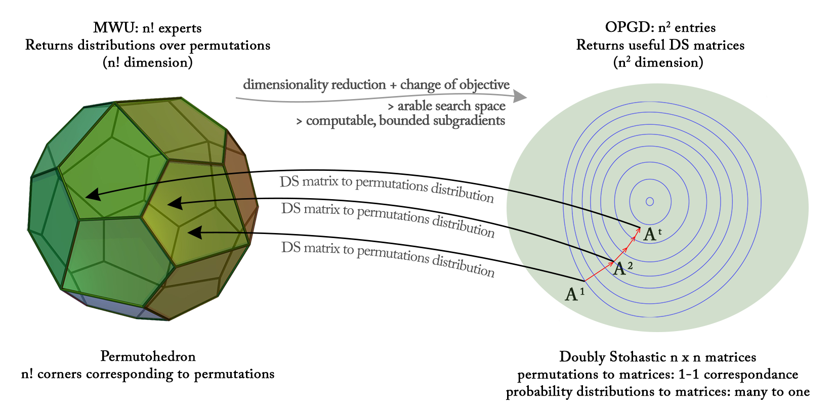
Figure 1: Our general approach, which is independent of the specific variant of $\mathrm{GMSSC}$.

Designing and Solving the Relaxed Online Learning Problem. For the relaxed version of $\mathrm{GMSSC}$, we note that any permutation $\pi$ corresponds to an integral doubly stochastic matrix $A^{\pi}$, with $A^{\pi}[i,j]=1$ iff $\pi(j)=i$. Moreover for any request $R$, each doubly stochastic matrix is associated with a fractional access cost. For integral doubly stochastic matrices, the fractional access cost is practically identical to the access cost of $\mathrm{GMSSC}$ in the respective permutation.

The fractional access cost is given by the optimal solution of an (exponentially large) configuration linear program (LP) that relaxes $\mathrm{GMSSC}$ to doubly stochastic matrices (see also [30]), and is a convex function. Thus, we can use Online Projected Gradient Descent (OPGD) [44] to produce a no-regret sequence of doubly stochastic matrices for the $\mathrm{GMSSC}$ relaxation. However, the efficient computation of the subgradient is far from trivial, due to the exponential size of the configuration LP. A key technical step is to show that the subgradient of the configuration LP can be computed in polynomial time, by solving its dual (which is of exponential size, so we resort to the elipsoid method and use an appropriate separation oracle).

Our Results. In nutshell, we resolve Question 1 in the affirmative. In addition to solving the relaxed version of $\mathrm{GMSSC}$ by a polynomial-time no-regret online learning algorithm, as described above, we present a polynomial-time randomized rounding scheme that maps any doubly stochastic matrix to a probability distribution on permutations. The expected access cost of such a probability distribution is at most $28$ times the fractional access cost of the corresponding doubly stochastic matrix. Consequently, a $28$-regret polynomial-time randomized online learning algorithm for $\mathrm{GMSSC}$ can be derived by applying, in each round, this rounding scheme to the doubly stochastic matrix $A^{t}$, produced by OPGD. For the important special case of $\mathrm{MSSC}$, we improve the regret bound to $11.713$ via a similar randomized rounding scheme that exploits the fact that $\mathrm{K}(R)=1$ for all requests.

We also present a polynomial-time deterministic rounding scheme mapping any (possibly fractional) doubly stochastic matrix to permutations. As before, applying this scheme to the sequence of doubly stochastic matrices produced by OPGD for the relaxation of $\mathrm{GMSSC}$ leads to a polynomial-time deterministic online learning algorithm with regret $2\max_{t}|R_{t}|$ for $\mathrm{MSSC}$. Such a nontrivial upper bound on the regret of deterministic online learning algorithms is rather surprising. Typically, learners that select their actions deterministically fail to achieve any nontrivial regret bounds (e.g., recall that in Learning From Expert Advice, any deterministic online algorithm has $\Omega(\#\text{experts})$ regret, which in case of $\mathrm{MSSC}$ is $n!$). Although $2\max_{t}|R_{t}|$ is not constant, one should expect that the requests are rather small in most practical applications. The above result is approximately tight, since any deterministic online learning algorithm must have regret at least $\max_{t}|R_{t}|/2$ [17, Theorem 1.1]. We should also highlight that the positive results of [17] do not imply the existence of computationally efficient online learning algorithms for $\mathrm{MSSC}$, because their approach is based on the MWU algorithm and uses a state space of $n!$. The state of the art and our results (in bold) are summarized below.

	Running Time	Upper Bound (Regret)	Lower Bound (Regret)
GMSSC	Exponential ($\mathrm{MWU}$)	1	1
GMSSC	Polynomial	$\bm{28}$	4 (any polynomial time)
MSSC	Polynomial	$\bm{11.713}$	4 (any polynomial time)
MSSC	Exponential (deterministic)	$2\cdot\max_{t}|R_{t}|$	$\frac{\max_{t}|R_{t}|}{2}$ (any deterministic)
MSSC	Polynomial (deterministic)	$\bm{2\cdot\max_{t}|R_{t}|}$	$\frac{\max_{t}|R_{t}|}{2}$ (any deterministic)

Related Work. Our work relates with the long line of research concerning the design of time-efficient online learning algorithms in various combinatorial domains in which the number of possible actions is exponentially large. Such domains include online routing [26, 3], selection of permutations [40, 42, 2, 27], selection of binary search trees [41], submodular minimization/maximization [23, 31, 37], matrix completion [24], contextual bandits [1, 11] and many more.

Apart from the above line of works, concerning the design of time-efficient online learning algorithms in specific settings, another line of research studies the design of online learning algorithms considering black-box access in offline algorithms [33, 35, 39, 34, 15, 10, 25, 32, 18, 19, 22]. In their seminal work [33], Kalai et al. showed how a polynomial-time algorithm solving optimally the underlying combinatorial problem, can be converted into a no-regret polynomial-time online learning algorithm. The result of Kalai et al. was subsequently improved [35, 39, 34] for settings in which the underlying problem can be (optimally) solved by a specific approach, such as dynamic programming. Although there do not exist such general reductions for $\alpha$-approximation (offline) algorithms (without taking into account the combinatorial structure of each specific setting [25]), Kakade et al. presented such a reduction for the (fairly general) class of linear optimization problems [32]. Their result was subsequently improved by [18, 19, 22]. We remark that the above results do not apply in our setting since $\mathrm{GMSSC}$ can neither be optimally solved in polynomial-time nor is a linear optimization problem.

Finally our works also relates with a recent line of research studying time-efficient online learning algorithms in settings related to selection of permutations and rankings [42, 2, 27, 38, 43]. The setting considered in [42, 2, 27] is very similar to $\mathrm{GMSSC}$ with the difference that once request $R_{t}$ is revealed, the learner pays the sum of the positions of $R_{t}$’s elements in permutation $\pi_{t}$. In this case the underlying combinatorial optimization problem can be solved in polynomial-time meaning that the reduction of [33] produces a time-efficient no-regret online learning algorithm. As a result, all the above works focus on improving the vanishing rate of time-average regret. The setting considered in [38] is based on the submodular maximization problem. In particular, the number of available positions is less than the number of elements, while the cost of the selected assignment depends on the set of elements assigned to the slots (their order does not matter). Although this problem is NP-hard, it admits an $(1-1/e)$-approximation algorithm which is matched by the presented online learning algorithm. Finally in [43], the cost of the selected permutation is its distance from a permutation selected by the adversary. In this case the underlying combinatorial optimization problem admits an offline $11/9$-approximation algorithm, while a polynomial-time online learning algorithm with $3/2$-regret is presented. We note that $\mathrm{GMSSC}$ admits a fairly more complicated combinatorial structure from the above settings and this is indicated by its $4$ inapproximability result.

2 Definitions and Notation

Definition 1 (Subgradient).

Given a function $f:D\mapsto\mathbb{R}$, with $D\subseteq\mathbb{R}^{n}$, a vector $g\in\mathbb{R}^{n}$ is a subgradient of $f$ at point $x\in\mathbb{R}^{n}$, denoted $g\in\partial F(x)$, if $f(y)\geq f(x)+g^{\top}(y-x)\leavevmode\nobreak\$, for all $y\in D$.

A matrix $A\in[0,1]^{n\times n}$ is doubly stochastic, if (i) $A_{ij}\geq 0$, for all $1\leq i,j\leq n$, (ii) $\sum_{i=1}^{n}A_{ij}=1$, for all $1\leq j\leq n$, and (iii) $\sum_{j=1}^{n}A_{ij}=1$, for all $1\leq i\leq n$. We let $\mathrm{DS}$ denote the set of $n\times n$ doubly stochastic matrices.

Any permutation $\pi\in[n!]$ can be represented by an integral doubly-stochastic $A^{\pi}$, where $A_{ij}^{\pi}=1$ iff $\pi(j)=i$. Under this representation, the access cost of $\mathrm{GMSSC}$, defined in (1), becomes:

$$\operatorname{AccessCost}(\pi,R)=\sum_{i=1}^{n}\min\left\{1,{\left(\mathrm{K(R)}-\sum_{j=1}^{i-1}\sum_{e\in R}A_{ej}^{\pi}\right)\!\!}_{+}\,\,\,\right\}\,,$$ (2)

where we define $(x-y)_{+}=\max\{x-y,0\}$.

A key notion for our algorithms and analysis is that of configurations. Given a request $R\subset U$, a configuration $F$ is an assignment of the elements $e\in R$ to positions $j\in[n]$ such that no two elements $e,e^{\prime}\in R$ share the same position. Intuitively, a configuration wrt. a request $R$ is the set of all permutations $\pi\in[n!]$ with the elements of $R$ in the exact same positions as indicated by $F$. As a result, all permutations $\pi\in[n!]$ that agree with a configuration $F$ wrt. a request $R$ have the same $\operatorname{AccessCost}(\pi,R)$. In the following, $\mathrm{F}(R)$ denotes the set of all configurations wrt. a request $R$ and $C_{F}$ denotes the access cost $\operatorname{AccessCost}(\pi,R)$ of any permutation $\pi\in[n!]$ that agrees with the configuration $F\in\mathrm{F}(R)$.

Example 1.

Let $R=\{2,5,7\}$ with $\mathrm{K}(R)=2$. The configuration $F_{1}=\{(2,3),(5,1),(7,10)\}$ stands for the set of permutations $\pi\in[n!]$ in which (i) $\pi(3)=2$, (ii) $\pi(1)=5$, and (iii) $\pi(10)=7$. The configuration $F_{1}$ is valid (i.e., $F_{1}\in\mathrm{F}(R)$), because no elements of $R$ share the same position. Moreover, $\mathrm{C}_{F_{1}}=3$, because any permutation $\pi$ agreeing with $F$ has cost $3$ for $\mathrm{K}(R)=2$. Similarly, for the configuration $F_{2}=\{(2,3),(5,1),(7,2)\}$, $C_{F_{2}}=2$.

3 Solving a Relaxation of Generalized Min-Sum Set Cover

Next, we present an online learning problem for a relaxed version of $\mathrm{GMSSC}$ in the space of doubly stochastic matrices. Specifically, we consider an online learning setting where, in each round $t\geq 1$,

1. The learner selects a doubly stochastic matrix $A^{t}\in\mathrm{DS}$.

2. The adversary selects a request $R_{t}$ with covering requirements $\mathrm{K}(R_{t})$.

3. The learner incurs the fractional access cost $\mathrm{FAC}_{R_{t}}(A^{t})$ presented in Definition 2.

Definition 2 (Fractional Access Cost).

Given a request $R$ with covering requirements $\mathrm{K}(R)$, the fractional access cost of a doubly stochastic matrix $A$, denoted as $\mathrm{FAC}_{R}(A)$ is the value of the following linear program:

$$\begin{array}[]{lr@{}ll}\mbox{\emph{minimize}}&\displaystyle\sum_{F\in\mathrm{F}(R)}C_{F}\cdot y_{F}&\,\,+\,\,\displaystyle\frac{n^{4}}{\epsilon}\cdot\sum\limits_{e\in R}\sum\limits_{j=1}^{n}|A_{ej}-\sum\limits_{F:(e,j)\in F}y_{F}|&\\ \mbox{\emph{subject to}}&\displaystyle\sum\limits_{\mathrm{F}\in\mathrm{F}(R)}y_{F}&=1\\ &y_{F}&\geq 0,\,\,\forall F\in\mathrm{F}(R)\end{array}$$ (FLP)

We always assume a fixed accuracy parameter $\epsilon$ (see also Theorem 1 about the role of $\epsilon$). Hence, for simplicity, we always ignore the dependence of $\mathrm{FAC}_{R}(A)$ on $\epsilon$. We should highlight that we need to deviate from the configuration LP of [30, Sec. 2], because OPGD requires an upper bound in the subgradient’s norm. The $n^{4}$ term in (FLP) was appropriately selected so as to ensure that the access cost of the probability distribution on permutations produced by a doubly stochastic matrix is upper bounded by its fractional access cost (see Section B.1).

An important property of the fractional access cost in Definition 2 is that for all integral doubly stochastic matrices, it is bounded from above by the access cost of $\mathrm{GMSSC}$ in (2). For that, simply note that a feasible solution is setting $y_{F}=1$ only for the configuration that “agrees” in the resources of $R$ with the permutation of the integral matrix $A$.

Corollary 1.

For any integral doubly stochastic matrix $A^{\pi}$ corresponding to a permutation $\pi\in[n!]$,

$$\mathrm{FAC}_{R}(A^{\pi})\leq\operatorname{AccessCost}(\pi,R).$$

For $A^{1},A^{2}\in\mathrm{DS}$, it is $\mathrm{FAC}_{R_{t}}\left(\lambda A^{1}+(1-\lambda)A^{2}\right)\leq\lambda\cdot\mathrm{FAC}_{R_{t}}\left(A^{1}\right)+(1-\lambda)\cdot\mathrm{FAC}_{R_{t}}\left(A^{2}\right)$, meaning that $\mathrm{FAC}_{R_{t}}(\cdot)$ is a convex function in the space of doubly stochastic matrices. Since doubly stochastic matrices form a convex set, Online Projected Gradient Descent [44] is a no-regret online learning algorithm for the relaxed version of $\mathrm{GMSSC}$.

3.1 Implementing Online Gradient Descent in Polynomial-time

Online Gradient Descent requires, in each round $t$, the computation of a subgradient of the fractional access cost $\mathrm{FAC}_{R_{t}}(A_{t})$ (see also Definition 1). Specifically, given a request $R$ and a doubly stochastic matrix $A$, a vector $g\in\mathbb{R}^{n^{2}}$ belongs to the subgradient $\partial\mathrm{FAC}_{R}(A)$, if for any $B\in\mathrm{DS}$,

$$\mathrm{FAC}_{R}(B)\geq\mathrm{FAC}_{R}(A)+g^{\top}(B-A)\,,$$ (3)

where we slightly abuse the notation and think of matrices $A$ and $B$ as vectors in $[0,1]^{n^{2}}$.

Computing a subgradient $g\in\partial\mathrm{FAC}_{R}(A)$ in polynomial-time is far from trivial, because the fractional access cost $\mathrm{FAC}_{R}(A)$ does not admit a closed form, since its value is determined by the optimal solution to (FLP). Moroever, (FLP) has exponentially many variables $y_{F}$, one for each configuration $F\in\mathrm{F}(R)$. We next show how to compute a subgradient $g\in\partial\mathrm{FAC}_{R}(A)$ by using linear programming duality and solving the dual of (FLP), which is presented below:

$$\begin{array}[]{lr@{}ll}\text{maximize}&\displaystyle\lambda+\sum_{e\in R}\sum_{j=1}^{n}A_{ej}\cdot\lambda_{ej}&\\ \text{subject to}&\displaystyle\lambda+\sum\limits_{(e,j)\in F}\lambda_{ej}&\leq C_{F},\text{ for all }F\in\mathrm{F}(R)\\ &|\lambda_{ej}|&\leq n^{4}/\epsilon\end{array}$$ (4)

Lemma 1.

For any request $R$ and any stochastic matrix $A\in\mathrm{DS}$, let $g\in\mathbb{R}^{n^{2}}$ denote the vector consisting of the $n^{2}$ values of the variables $\lambda^{\ast}_{ej}$ in the optimal solution of (4). Then, for any $B\in\mathrm{DS}$,

$$\mathrm{FAC}_{R}(B)\geq\mathrm{FAC}_{R}(A)+g^{\top}(B-A)$$

Moreover the Euclidean norm of $g$ is upper bounded by $n^{5}/\epsilon$, i.e., $\lVert g\rVert_{2}\leq n^{5}/\epsilon$.

Lemma 1 shows that a subgradient $g\in\partial\mathrm{FAC}_{R}(A)$ can be obtained from the solution to the dual LP (4). Although (4) has exponentially many constraints, we can solve it in polynomial-time by the ellipsoid method, through the use of an appropriate separation oracle. In fact, our separation oracle results from a simple modification of the separation oracle in [30, Sec. 2.3] (see also Section A). Now, the reasons for the particular form of fractional access cost in Definition 2 become clear: (i) it allows for efficient computation of the subgradients, and (ii) the dual constraints $|\lambda_{ej}|\leq n^{4}/\epsilon$ imply that the subgradient’s norm is always bounded by $n^{5}/\epsilon$.

Remark 1.

For the Min-Sum Set Cover problem, the use of the ellipsoid method (for the computation of the subgradient vector) can be replaced by a more efficient quadratic-time algorithm (see Appendix B.2).

Having established polynomial-time computation for the subgradients, Online Projected Gradient Descent takes the form of Algorithm 1 in our specific setting.

Algorithm 1 Online Projected Gradient Decent in Doubly Stochastic Matrices

1:Initially, the player selects the matrix $A^{1}=1/n\cdot 1_{n\times n}$.

2:for all  rounds $t=1\cdots T$ do

3:     The adversary selects a request $R_{t}\subseteq U$ with covering requirements $\mathrm{K}(R_{t})$.

4:     The learner receives cost, $\mathrm{FAC}_{R_{t}}(A^{t})$.

5:     The learner computes a subgradient $g_{t}\in\partial\mathrm{FAC}_{R_{t}}(A^{t})$ by solving the dual of (FLP).

6:     The learner computes the matrix, $\hat{A}=A^{t}-2\epsilon\cdot g_{t}/(n^{4.5}\sqrt{t})$.

7:     The learner adopts the matrix, $A^{t+1}=\operatorname*{arg\,min}_{A\in\mathrm{DS}}\lVert A-\hat{A}\rVert_{\mathrm{F}}$

8:end for

Step $6$ of Algorithm 1 is the gradient step. In Online Projected Gradient Descent, this step is performed with step-size $D/(G\sqrt{t})$, where $D$ and $G$ are upper bounds on the diameter of the action space and on the Euclidean norm of the subgradients. In our case, the action space is the set of doubly stochastic matrices. Since $\max_{A,B\in\mathrm{DS}}\lVert A-B\rVert_{\mathrm{F}}\leq 2\sqrt{n}$ the parameter $D=2\sqrt{n}$, and $G=n^{5}/\epsilon$, by Lemma 1. Hence, our step-size is $2\epsilon/(n^{4.5}\sqrt{t})$. The projection step (Step $7$) is implemented in polynomial-time, because projecting to doubly stochastic matrices is a convex problem [16]. We conclude the section by plugging in the parameters $G=n^{5}/\epsilon$ and $D=2\sqrt{n}$ to the regret bounds of Online Projected Gradient Descent [44], thus obtaining Theorem 1.

Theorem 1.

For any $\epsilon>0$ and any request sequence $R_{1},\ldots,R_{T}$, the sequence of doubly stochastic matrices $A^{1},\ldots,A^{T}$ produced by Online Projected Gradient Descent (Algorithm 1) satisfies, $\frac{1}{T}\sum_{t=1}^{T}\mathrm{FAC}_{R_{t}}(A^{t})\leq\frac{1}{T}\min_{A\in\mathrm{DS}}\sum_{t=1}^{T}\mathrm{FAC}_{R_{t}}(A)+O\left(\frac{n^{5.5}}{\epsilon\sqrt{T}}\right)$.

4 Converting Doubly Stochastic Matrices to Distributions on Permutations

Next, we present polynomial-time rounding schemes that map a doubly stochastic matrix back to a probability distribution on permutations. Our schemes ensure that the resulting permutation (random or deterministic) has access cost at most $\alpha$ times the fractional access cost of the corresponding doubly stochastic matrix. Combining such schemes with Algorithm 1, we obtain polynomial-time $\alpha$-regret online learning algorithms for $\mathrm{GMSSC}$.

Due to lack of space, we only present the deterministic rounding scheme, which is intuitive and easy to explain. Most of its analysis and the description of the randomized rounding schemes are deferred to the supplementary material.

Algorithm 2 Converting Doubly Stochastic Matrices to Permutations

Input: A doubly stochastic matrix $A\in\mathrm{DS}$, a parameter $r$ and a parameter $\alpha>0$.
Output: A deterministic permutation $\pi_{A}\in[n!]$.

1:$\text{Rem}\leftarrow\{1,\ldots,n\}$

2:for $k=1$ to $\left\lfloor{n/r}\right\rfloor$  do

3:     Let $R_{k}$ be any $(1+\alpha)$-approximate solution to the following problem:

$$\min_{R\subseteq\mathrm{Rem}:|R|=r}\,\,\sum_{i=1}^{n}{\left(1-\sum_{j=1}^{i-1}\sum_{e\in R}A_{ej}\right)\!\!}_{+}$$

4:     Assign the elements of $R_{k}$ to positions $(k-1)\cdot r+1,\ldots,k\cdot r$ of $\pi_{A}$ in any order.

5:     $\text{Rem}\leftarrow\text{Rem}\setminus R_{k}$

6:end for

7:return the resulting permutation $\pi_{A}\in[n!]$.

Algorithm 2 aims to produce a permutation $\pi_{A}\in[n!]$ from the doubly stochastic matrix $A$ such that the $\operatorname{AccessCost}(\pi_{A},R)$ is approximately bounded by $\mathrm{FAR}_{R}(A)$ for any request $R$ with $|R|\leq r$ and $\mathrm{K}(R)=1$. Algorithm 2 is based on the following intuitive greedy criterion:

Assign to the first $r$ available positions of $\pi_{A}$ the elements of the request of size $r$ with minimum fractional cost of Definition 2 wrt. the doubly stochastic matrix $A$. Then, remove these elements and repeat.

Unfortunately the greedy step above involves the solution to an $\mathrm{NP}$-hard optimization problem. Nevertheless, we can approximate it with an FPTAS (Fully Polynomial-Time Approximation Scheme). The (1+$\alpha$)-approximation algorithm used in Step $3$ of Algorithm 2 runs in $\Theta(n^{4}r^{3}/\alpha^{2})$ and is presented and analyzed in Section B.5. Theorem 2 (proved in Section B.3) summarizes the guarantees on the access cost of a permutation $\pi_{A}$ produced by Algorithm 2.

Theorem 2.

Let $\pi_{A}$ denote the permutation produced by Algorithm 2 when the doubly stochastic matrix $A$ is given as input. Then for any request $R$ with $\mathrm{K}(R)=1$ and $|R|\leq r$,

$$\operatorname{AccessCost}(\pi_{A},R)\leq 2(1+\epsilon)(1+\alpha)^{2}r\cdot\mathrm{FAC}_{R}(A),$$

with $\epsilon>0$ as in Definition 2. Moreover, Step $3$, can be implemented in $\Theta(n^{4}r^{3}/\alpha^{2})$ steps.

We now show how Algorithm 1 and Algorithm 2 can be combined to produce a polynomial-time deterministic online learning algorithm for $\mathrm{MSSC}$ with regret roughly $2\max_{1\leq t\leq T}|R_{t}|$. For any adversarially selected sequence of requests $R_{1},\ldots,R_{T}$ with $\mathrm{K}(R_{t})=1$ and $|R_{t}|\leq r$, the learner runs Algorithm 1 in the background, while at each round $t$ uses Algorithm 2 to produce the permutation $\pi_{A^{t}}$ by the doubly stochastic matrix $A^{t}\in\mathrm{DS}$. Then,

$$\frac{1}{T}\sum_{t=1}^{T}\operatorname{AccessCost}(\pi_{A^{t}},R_{t}) \leq \frac{1}{T}\cdot\sum_{t=1}^{T}2(1+\epsilon)(1+\alpha)^{2}r\cdot\mathrm{FAC}_{R_{t}}(A^{t})$$

$$\leq \frac{2r}{T}(1+\epsilon)(1+\alpha)^{2}\cdot\min_{A\in\mathrm{DS}}\sum_{t=1}^{T}\mathrm{FAC}_{R^{t}}(A)+O\left(\frac{n^{5.5}}{\epsilon\sqrt{T}}\right)$$

$$\leq \frac{2r}{T}(1+\epsilon)(1+\alpha)^{2}\cdot\sum_{t=1}^{T}\mathrm{FAC}_{R^{t}}(A^{\pi^{\ast}})+O\left(\frac{n^{5.5}}{\epsilon\sqrt{T}}\right)$$

$$\leq \frac{2r}{T}(1+\epsilon)(1+\alpha)^{2}\cdot\sum_{t=1}^{T}\operatorname{AccessCost}(\pi^{\ast},R^{t})+O\left(\frac{n^{5.5}}{\epsilon\sqrt{T}}\right)$$

The first inequality follows by Theorem 2, the second by Theorem 1 and the last by Corollary 1.

Via the use of randomized rounding schemes we can substantially improve both on the assumptions and the guarantee of Theorem 2. Algorithm 3 (presented in Section B.1), describes such a scheme that converts any doubly stochastic matrix $A$ to a probability distribution over permutations, while Theorem 3 (also proven in Section B.1) establishes an approximation guarantee (arbitrarily) close to $28$ on the expected access cost.

Theorem 3.

Let $\mathrm{P_{A}}$ denote the probability distribution over permutations that Algorithm 3 produces given as input an $A\in\mathrm{DS}$. For any request $R$,

$$\mathop{{}\mathbb{E}}_{\pi\sim\mathrm{P_{A}}}[\operatorname{AccessCost}(\pi,R)]\leq 28(1+\epsilon)\cdot\mathrm{FAC}_{R}(A)$$

where $\epsilon>0$ is the parameter used in Definition 2.

Using Theorem 3 instead of Theorem 2 in the previously exhibited analysis, implies that combining Algorithms 1 and  3 leads to a polynomial-time randomized online learning algorithm for $\mathrm{GMSSC}$ with $28(1+\epsilon)$ regret.

In Section B.2 we improve Theorem 3 for the the special case of $\mathrm{MSSC}$. The randomized rounding scheme described in Algorithm 4 admits the approximation guarantee of Theorem 4, which implies a polynomial-time randomized online learning algorithm for $\mathrm{MSSC}$ with $11.713(1+\epsilon)$ regret

Theorem 4.

Let $\mathrm{P_{A}}$ denote the probability distribution over permutations that Algorithm 4 produces given as input an $A\in\mathrm{DS}$. For any request $R$ with covering requirement $\mathrm{K}(R)=1$,

$$\mathop{{}\mathbb{E}}_{\pi\sim\mathrm{P}_{A}}[\operatorname{AccessCost}(\pi,R)]\leq 11.713(1+\epsilon)\cdot\mathrm{FAC}_{R}(A)$$

where $\epsilon>0$ is the parameter used in Definition 2.

5 Experimental Evaluations

In this section we provide experimental evaluations of all the proposed online learning algorithms (both deterministic and randomized) for Min-Sum Set Cover. Surprisingly enough our simulations seem to suggest that the deterministic rounding scheme proposed in Algorithm 2, performs significantly better than its theoretical guarantee, stated in Theorem 2, that associates its regret with the cardinality of the sets. The following figures illustrate the performance of Algorithm 2 and Algorithm 4, and compare it with the performance of the offline algorithm proposed by Feige et al. [13] and the performance of selecting a permutation uniformly at random at each round. In the left figure each request contains either element $1$ or $2$ and four additional randomly selected elements, while in the right figure each request contains one of the elements $\{1,2,3,4,5\}$ and nine more randomly selected elements. We remark that in our experimental evaluations, we solve the optimization problem of Step $3$ in Algorithm 2 through a simple heuristic that we present in Appendix B.6, while for the computation of the subgradients we use the formula presented in Corollary 3. The code used for the presented simulations can be found at https://github.com/sskoul/ID2216.

6 Conclusion

This work examines polynomial-time online learning algorithms for (Generalized) Min-Sum Set Cover. Our results are based on solving a relaxed online learning problem of smaller dimension via Online Projected Gradient Descent, the solution of which is transformed at each round into a solution of the initial action space with bounded increase in the cost. To do so, the cost function of the relaxed online learning problem is defined by the value of a linear program with exponentially many constraints. Despite its exponential size, we show that the subgradients can be efficiently computed via associating them with the variables of the LP’ s dual. We believe that the bridge between online learning algorithms (e.g. online projected gradient descent) and traditional algorithmic tools (e.g. duality, separation oracles, deterministic/randomized rounding schemes), introduced in this work, is a promising new framework for the design of efficient online learning algorithms in high dimensional combinatorial domains. Finally closing the gap between our regret bounds and the lower bound of $4$, which holds for polynomial-time online learning algorithms for $\mathrm{MSSC}$, is an interesting open problem.

Broader Impact

We are living in a world of abundance, where each individual is provided myriad of options in terms of available products and services (e.g. music selection, movies etc.). Unfortunately this overabundance makes the cost of exploring all of them prohibitively large. This problem is only compounded by the fast turn around of new trends at a seemingly ever increasing rate. Our algorithmic techniques provide a practically applicable methodology for managing this complexity.

Funding Disclosure

Dimitris Fotakis and Thanasis Lianeas are supported by the Hellenic Foundation for Research and Innovation (H.F.R.I.) under the “First Call for H.F.R.I. Research Projects to support Faculty members and Researchers’ and the procurement of high-cost research equipment grant”, project BALSAM, HFRI-FM17-1424. Stratis Skoulakis was supported by NRF 2018 Fellowship NRF-NRFF2018-07. G. Piliouras gratefully acknowledges AcRF Tier-2 grant (Ministry of Education – Singapore) 2016-T2-1-170, grant PIE-SGP-AI-2018-01, NRF2019-NRF-ANR095 ALIAS grant and NRF 2018 Fellowship NRF-NRFF2018-07 (National Research Foundation Singapore).

Appendix A Omitted Proofs of Section 3

Proof of Lemma 1.

To simplify notation, let $\lambda^{\ast}(A),\lambda^{\ast}_{ej}(A)$ denote the values of the variables $\lambda^{\ast}(A),\lambda^{\ast}(A)_{ej}$ in the optimal solution of the dual program written with respect to doubly stochastic matrix $A\in\mathrm{DS}$. Respectively $\lambda^{\ast}(B),\lambda_{ej}^{\ast}(B)$ for the doubly stochastic matrix $B\in\mathrm{DS}$. By strong duality, we have that

$$\mathrm{FAC}_{R}(A)=\lambda^{\ast}(A)+\sum_{e\in R}\sum_{j=1}^{n}A_{ej}\cdot\lambda^{\ast}_{ej}(A)\text{ and }\mathrm{FAC}_{R}(B)=\lambda^{\ast}(B)+\sum_{e\in R}\sum_{j=1}^{n}B_{ej}\cdot\lambda^{\ast}_{ej}(B)$$

Since matrices $A$ and $B$ only affect the objective function of the dual and not its constraints, the solution $\lambda^{\ast}(A),\lambda_{ej}^{\ast}(A)$ is a feasible solution for the dual program written according to matrix $B$. By the optimality of $\lambda^{\ast}(B),\lambda^{\ast}_{ej}(B)$ we get,

$$\mathrm{FAC}_{R}(B)=\lambda^{\ast}(B)+\sum_{e\in R}\sum_{j=1}^{n}B_{ej}\cdot\lambda^{\ast}_{ej}(B)\geq\lambda^{\ast}(A)+\sum_{e\in R}\sum_{j=1}^{n}B_{ej}\cdot\lambda^{\ast}_{ej}(A)$$

As a result, we get that $\mathrm{FAC}_{R}(B)-\mathrm{FAC}_{R}(A)\geq\sum_{e\in R}\sum_{j=1}^{n}\lambda^{\ast}_{ej}(A)\cdot(B_{ej}-A_{ej})$ implying that the vector $g$ containing the $\lambda^{\ast}_{ej}(A)$’s, is a subgradient of $\mathrm{FAC}_{R}(\cdot)$ at point $A$, i.e., $g\in\partial\mathrm{FAC}_{R}(A)$. The inequality $\lVert g\rVert_{2}\leq n^{5}/\epsilon$ directly follows by the fact that $|\lambda^{\ast}(A)_{ej}|\leq n^{4}/\epsilon$. ∎

Separation Oracle for the LP in Equation 4: The dual linear program of (4) is differs from the $\text{LP}_{\text{dual}}$ in [30, Sec. 2.2] only in the constraints $|\lambda_{ej}|\leq n^{4}/\epsilon$, which are only present in (4). [30, Sec. 2.2] present a separation oracle for their $\text{LP}_{\text{dual}}$ (i.e., for (4), without the constraints $|\lambda_{ej}|\leq n^{4}/\epsilon$), which is based on formulating and solving a min-cost flow problem. Since, in case of (4), the we have only $n^{2}$ additional constraints $|\lambda_{ej}|\leq n^{4}/\epsilon$, we can first check whether these constraints are satisfied by the current solution and then run the separation oracle of [30].

Appendix B Omitted Proofs of Section 4

B.1 Proof of Theorem 3

In Algorithm 3, we present the online randomized rounding scheme that combined with Projected Gradient Descent (Algorithm 1) produces a polynomial-time randomized online learning algorithm for $\mathrm{GMSSC}$ with (roughly) $28$ regret. The randomized rounding scheme described in Algorithm 3 was introduced by [36] to provide a $28$-approximation algorithm for the (offline) $\mathrm{GMSSC}$. [36] proved that this randomized rounding scheme produces a random permutation with access cost at most $28$ times greater than the optimal fractional value of the LP relaxation of $\mathrm{GMSSC}$ introduced in [6]. We remark that this LP relaxation cannot be translated to an equivalent relaxed online learning problem as the one we formulated using the fractional access cost of Definition 2. The goal of the section is to prove Theorem 3 which extends the result of [36] to the fractional access cost of Definition 2.

Algorithm 3 Converting Doubly Stochastic Matrices to Probability Distributions over Permutations

Input: A doubly stochastic matrix $A\in\mathrm{DS}$.
Output: A probability distribution over permutations, $\mathrm{P}_{A}\sim\pi\in[n!]$

1:Randomly pick $\alpha\in(0,1)$ with probability density function $f(\alpha)=2\alpha$.

2:Set $B\leftarrow(5.03/\alpha)\cdot A$

3:for  all elements $e=1$ to $n$  do

4:     for  all positions $j=1$ to $\left\lfloor{n/2}\right\rfloor$  do

5:         $B_{e,2j}\leftarrow B_{e,2j}+B_{e,j}$.

6:     end for

7:end for

8:for  all elements $e=1$ to $n$  do

9:     Pick $\alpha_{e}$ uniformly at random in $[0,1]$.

10:     Find the effecive index $i_{e}^{\alpha}\leftarrow\operatorname*{arg\,max}_{i}\{i:\sum_{j=1}^{i-1}B_{ej}<\alpha_{e}\}$.

11:end for

12:Output the elements according to the order of $i_{e}$’s.

Definition 3.

For a request $R$ with covering requirements $\mathrm{K}(R)$, we define the cost $\mathrm{SW}_{R}:\mathrm{DS}\mapsto\mathbb{R}$ on the doubly stochastic matrices as follows: For any doubly stochastic matrix $A\in\mathrm{DS}$, the value $\mathrm{SW}_{R}(A)$ equals the value of the following linear program,

$$\begin{array}[]{ll@{}ll}\text{minimize}&\displaystyle\sum_{i=1}^{n}\left(1-z_{i}\right)&\\ \text{subject to}&\displaystyle\left(\mathrm{K}(R)-|M|\right)\cdot z_{i}\leq\sum\limits_{j=1}^{i-1}\sum\limits_{e\in R\setminus M}A_{ej}\leavevmode\nobreak\ \text{ for all }\leavevmode\nobreak\ M\subseteq R\\ &z_{i}\in[0,1]\leavevmode\nobreak\ \text{ for all}\leavevmode\nobreak\ 1\leq i\leq n\end{array}$$

Lemma 2.

[36] For any doubly stochastic matrix $A\in\mathrm{DS}$,

$$\mathop{{}\mathbb{E}}_{\pi\sim\mathrm{P}_{A}}[\operatorname{AccessCost}(\pi,R)]\leq 28\cdot\mathrm{SW}_{R}(A)$$

where $\mathrm{P}_{A}$ is the probability distribution over the permutation produced by Algorithm 3 when the matrix $A$ was given as input.

In Lemma 3 we associate the cost $\mathrm{SW}_{R}(\cdot)$ of Definition 3 with the fractional access cost $\mathrm{FAC}_{R}(\cdot)$ of Definition 2. Then Theorem 3 directly follows by Lemma 2 and Lemma 3.

Lemma 3.

For any doubly stochastic matrix $A\in\mathrm{DS}$,

$$\mathrm{SW}_{R}(A)\leq(1+\epsilon)\cdot\mathrm{FAC}_{R}(A)$$

where $\epsilon>0$ is the parameter of the linear program (FLP) in Definition 2.

Proof.

Starting from the optimal solution $y_{F}$ of the linear program (FLP) of $\mathrm{FAC}_{R}(A)$ in Definition 2, we construct a feasible solution for the linear program of $\mathrm{SW}_{R}(A)$ of Definition 3 with cost approximately bounded by $(1+\epsilon)\cdot\mathrm{FAC}_{R}(A)$. We first prove Claim 1 that is crucial for the subsequent analysis.

Claim 1.

For any element $e\in R$ and position $1\leq j\leq n$, $|A_{ej}-\sum\limits_{F:(e,je,e,j)\in F}y_{F}^{\ast}|\leq\epsilon/n^{3}$.

Proof.

Since $A$ is a doubly stochastic matrix, by the Birkhoff-von Neumann theorem there exists a vector $\hat{y}$ with $\hat{y}_{F}\geq 0$ and $\sum_{F\in\mathrm{F}(R)}\hat{y}_{F}=1$ such that

$$|A_{ej}-\sum\limits_{F:(e,j)\in F}\hat{y}_{F}|=0\text{ for all }e\in R\text{ and }1\leq j\leq n$$

Since $y^{\ast}$ is the optimal solution, we have that

$$\sum_{F\in\mathrm{F}(R)}C_{F}\cdot y_{F}^{\ast}+\frac{n^{4}}{\epsilon}\cdot\sum_{e\in R}\sum_{j=1}^{n}|A_{ej}-\sum\limits_{F:(e,j)\in F}y_{F}^{\ast}|\leq\sum_{F\in\mathrm{F}(R)}C_{F}\cdot\hat{y}_{F}.$$

Now the claim follows by the fact that $1\leq C_{F}\leq n$, $\hat{y}_{F}\geq 0$ and $\sum_{F\in\mathrm{F}(R)}\hat{y}_{F}=1$. ∎

Having established Claim 1, we construct the solution $z^{\ast}$ that is feasible for the linear program of Definition 3 and its value (under the linear program of Definition 3), is upper bounded by $(1+\epsilon)\cdot\mathrm{FAC}_{R}(A)$. For each position $1\leq i\leq n$,

$$z_{i}^{\ast}=\left(\sum_{F\in\mathrm{F}(R):C_{F}\leq i-1}y_{F}^{\ast}-\frac{\epsilon}{n}\right)_{+}$$

We first prove that $z^{\ast}$ is feasible for the linear program of Definition 3. At first observe that in case $z_{i}^{\ast}=0$ or $\mathrm{K}(R)-|M|\leq 0$ for some $M\subseteq R$, the constraint $\left(\mathrm{K}(R)-|M|\right)\cdot z_{i}\leq\sum_{j=1}^{i-1}\sum_{e\in R\setminus M}A_{ej}$ is trivially satisfied. We thus turn our attention in the cases where $z_{i}^{\ast}=\sum_{F:C_{F}\leq i-1}y_{F}^{\ast}-\epsilon/n>0$ and $K(R)-|M|\geq 1$ (recall, $K(R)$ and $|M|$ are integers). Applying Claim 1 we get that,

$$\sum_{e\in R\setminus M}\sum_{j=1}^{i-1}A_{ej} \geq \sum_{e\in R\setminus M}\sum_{j=1}^{i-1}\left(\sum_{F:(e,j)\in F}y_{F}^{\ast}-\epsilon/n^{3}\right)$$

$$\geq \sum_{e\in R\setminus M}\sum_{j=1}^{i-1}\sum_{F:(e,j)\in F}y_{F}^{\ast}-\epsilon/n$$

$$= \sum_{F\in\mathrm{F}(R)}y_{F}^{\ast}\sum_{e\in R\setminus M}\sum_{j=1}^{i-1}\textbf{1}[(e,j)\in F]-\epsilon/n$$

$$\geq \sum_{F:C_{F}<i}y_{F}^{\ast}\sum_{e\in R\setminus M}\sum_{j=1}^{i-1}\textbf{1}[(e,j)\in F]-\epsilon/n$$

$$\geq \left(K(R)-|M|\right)\sum_{F:C_{F}<i}y_{F}^{\ast}-\epsilon/n$$

$$= \left(K(R)-|M|\right)\cdot z_{i}^{\ast}+\epsilon\frac{K(R)-|M|}{n}-\epsilon/n$$

$$\geq \left(K(R)-|M|\right)\cdot z_{i}^{\ast}$$

where the second to last inequality follows from $C_{F}<i$, and the last equation and the last inequality follow from $z_{i}^{\ast}+\epsilon/n=\sum_{F:C_{F}\leq i-1}y_{F}^{\ast}$ and $\mathrm{K}(R)-|M|\geq 1$, respectively.

We complete the proof of Lemma 3 by showing that $\sum_{i=1}^{n}(1-z_{i}^{\ast})\leq(1+\epsilon)\cdot\mathrm{FAC}_{R}(A)$.

$$\mathrm{SW}_{R}(A) \leq \sum_{i=1}^{n}\left(1-z_{i}^{\ast}\right)$$

$$\leq \sum_{i=1}^{n}\left(1-\sum_{F:C_{F}<i}y_{F}^{\ast}+\epsilon/n\right)$$

$$= \sum_{i=1}^{n}\left(1-\sum_{F:C_{F}<i}y_{F}^{\ast}\right)+\epsilon$$

$$= \sum_{i=1}^{n}\sum_{F:C_{F}\geq i}y_{F}^{\ast}+\epsilon$$

$$= \sum_{F\in\mathrm{F}(R)}C_{F}\cdot y_{F}^{\ast}+\epsilon$$

$$\leq (1+\epsilon)\cdot\mathrm{FAC}_{R}(A)$$

∎

B.2 Proof of Theorem 4

We first present the online sampling scheme, described in Algorithm 4, that produces the $11.713$ guarantee of Theorem 4.

Algorithm 4 Converting Doubly Stochastic Matrices to Probability Distribution (the case of MSSC)

Input: A doubly stochastic matrix $A\in\mathrm{DS}$.
Output: A probability distribution over permutations, $\mathrm{P}_{A}\sim\pi\in[n!]$.

1:Randomly pick $\alpha\in(0,1)$ with probability density function $f(\alpha)=2\alpha$.

2:Set $B\leftarrow Q\cdot A$ where $Q\leftarrow 1.6783/\alpha$.

3:for  all elements $e=1$ to $n$  do

4:     for  all positions $j=1$ to $\left\lfloor{n/2}\right\rfloor$  do

5:         $B_{e,2j}\leftarrow B_{e,2j}+B_{e,j}$

6:     end for

7:end for

8:for  all elements $e=1$ to $n$  do

9:     Pick $\alpha_{e}$ uniformly at random in $[0,1]$.

10:     $i_{e}\leftarrow\max\{i:\sum_{j=1}^{i-1}B_{ej}<\alpha_{e}\}$

11:end for

12:Output the elements according to the order of $i_{e}$’s.

We dedicate the rest of the section to prove Theorem 4. Notice that Algorithm 4 is identical to Algorithm 3 with a slight difference in Step $2$. Taking advantage of $K(R)=1$, with tailored analysis, we significantly improve to $11.713$ the $28$ bound of Lemma 2. Once Lemma 4 below is established, Theorem 4 follows by the exact same steps that Theorem 3 follows using Lemma 2. The proof of Lemma 4 is concluded at the end of the section.

Lemma 4.

Let $\mathrm{P}_{A}$ denote the probability distribution over permutations produced by Algorithm 4 when matrix $A$ is given as input. For all requests $R$ with $\mathrm{K}(R)=1$,

$$\mathop{{}\mathbb{E}}_{\pi\sim\mathrm{P}_{A}}[\operatorname{AccessCost}(\pi,R)]\leq 11.713\cdot\mathrm{SW}_{R}(A)$$

where $\mathrm{SW}_{R}(\cdot)$ is the cost of Definition 3.

In fact $\mathrm{SW}_{R}(\cdot)$ takes a simpler form.

Corollary 2.

For any request $R$ with covering requirement $\mathrm{K}(R)=1$, the cost $\mathrm{SW}_{R}(\cdot)$ of Definition 3 takes the following simpler form,

$$\mathrm{SW}_{R}(A)=\sum_{i=1}^{n}\left(1-\sum_{j=1}^{i-1}\sum_{e\in R}A_{ej}\right)_{+}$$

Lemma 5.

[36] For the matrix $B$ constructed at Step $2$ of Algorithm 4, the following holds:

1. $\sum\limits_{j=1}^{2^{k}i}B_{ej}\geq(k+1)\sum\limits_{j=1}^{i}A_{ej}$

2. $\sum\limits_{j=1}^{i}\sum\limits_{e=1}^{n}B_{ej}\leq 2Q\cdot i$.

Condition $2$ of Lemma 5 allows for a bound on the expected access cost of the probability distribution produced by Algorithm 4 with respect to the indices $i_{e}$ of Step $10$. This is formally stated below.

Lemma 6.

Let $\mathrm{P}^{A}_{\alpha}$ denote the probability distribution produced in Steps $2-11$ of Algorithm 4 for a fixed value of $\alpha$. Then for any request $R$ with covering requirements $\mathrm{K}(R)=1$,

$$\mathop{{}\mathbb{E}}_{\pi\sim\mathrm{P_{\alpha}^{A}}}[\operatorname{AccessCost}(\pi,R)]\leq 2Q\cdot\mathop{{}\mathbb{E}}[\min_{e\in R}i_{e}]+1,$$

with $i_{e}$ as defined in Step $10$ of Algorithm 4.

Proof.

Let $O_{i}^{R}$ denote the set of elements outside $R$ with index value $i_{e}\leq i$,

$$O_{i}^{R}=\{e\notin R:\leavevmode\nobreak\ i_{e}\leq i\}.$$

Notice that Algorithm 4 orders the elements with respect to the values $i_{e}$ (Step $12$). Since the covering requirements of the request $R$ is $\mathrm{K}(R)=1$,

$$\operatorname{AccessCost}(\pi,R)\leq|O_{\min_{e\in R}i_{e}}^{R}|+1.$$

The latter holds since $R$ is covered at the first index in which one of its elements appears ($\mathrm{K}(R)=1$). As a result,

$$\mathop{{}\mathbb{E}}_{\pi\sim P^{A}_{\alpha}}[\operatorname{AccessCost}(\pi,R)]\leq\mathop{{}\mathbb{E}}[|O_{\min_{e\in R}i_{e}}^{R}|]+1\leq\sum_{e^{\prime}\notin R}\Pr[i_{e^{\prime}}\leq\min_{e\in R}i_{e}]+1$$

It is not hard to see that,

$$\sum_{e^{\prime}\notin R}\Pr[i_{e^{\prime}}\leq\min_{e\in R}i_{e}]+1=\mathop{{}\mathbb{E}}[\sum_{e^{\prime}\notin R}\sum_{j=1}^{\min_{e\in R}i_{e}}B_{e^{\prime}j}]+1\leq 2Q\cdot\mathop{{}\mathbb{E}}[\min_{e\in R}i_{e}]+1$$

where the first equality follows by the fact that, once $B$ is fixed, $\Pr[i_{e}\leq k]=\sum_{j=1}^{k}B_{ej}$ (Step 10 of Algorithm 4) and the last inequality follows by Case $2$ of Lemma 5. ∎

Lemma 7.

Let $i_{R}^{\alpha}$ denote the first position at which $\sum\limits_{j=1}^{i_{R}^{\alpha}}\sum\limits_{e\in R}A_{ej}\geq\alpha$ then

$$\int_{0}^{1}i_{R}^{\alpha}\leavevmode\nobreak\ d\alpha\leq\sum_{i=1}^{n}\left(1-\sum_{j=1}^{i-1}\sum_{e\in R}A_{ej}\right)_{+}=\mathrm{SW}_{R}(A)$$

Proof.

In order to prove Lemma 7, let us assume that a random variable $\beta$ is selected according to the uniform probability distribution in $[0,1]$, i.e., with density function $f(\beta)=1$. As a result, $\int_{0}^{1}i_{R}^{\alpha}\leavevmode\nobreak\ d\alpha=\int_{0}^{1}i_{R}^{\beta}\leavevmode\nobreak\ d\beta=\mathop{{}\mathbb{E}}[i_{R}^{\beta}]=\sum\limits_{i=1}^{n}\Pr[i_{R}^{\beta}\geq i]$. Since $i_{R}^{\beta}$ is the first position at which $\sum\limits_{j=1}^{i_{R}^{\beta}}\sum\limits_{e\in R}A_{ej}\geq\beta$,

$$\Pr[i^{\beta}_{R}\geq i]=\Pr[\beta>\sum_{j=1}^{i-1}\sum_{e\in R}A_{ej}]=\max\left(1-\sum_{j=1}^{i-1}\sum_{e\in S}A_{ej},0\right)\leq\sum_{i=1}^{n}\left(1-\sum_{j=1}^{i-1}\sum_{e\in R}A_{ej}\right)_{+}$$

with the second equality following because $\beta$ is selected according to the uniform distribution in $[0,1]$. ∎

To this end we have upper bounded the expected access cost of Algorithm 4 by $\mathop{{}\mathbb{E}}[\min_{e\in R}i_{e}]$ (Lemma 4) and lower bounded $\mathrm{SW}_{R}(A)$ by $\int_{0}^{1}i_{R}^{\alpha}\leavevmode\nobreak\ d\alpha$ (Lemma 7). In Lemma 8 we associate these bounds. At this point the role of Condition $1$ of Lemma 5 is revealed.

Lemma 8.

Let $i_{R}^{\alpha}$ denote the first position at which $\sum\limits_{j=1}^{i_{R}^{\alpha}}\sum\limits_{e\in R}A_{ej}\geq\alpha$ then

$$\mathop{{}\mathbb{E}}[\min_{e\in R}i_{e}]\leq i_{R}^{\alpha}/(1-2e^{-\alpha Q}).$$

Proof.

$$\Pr[\min_{e\in R}i_{e}\geq 2^{k}\cdot i_{R}^{\alpha}+1] = \Pi_{e\in R}\Pr[i_{e}\geq 2^{k}\cdot i_{R}^{\alpha}+1]$$

$$= \Pi_{e\in R}\Pr[\alpha_{e}>\sum\limits_{j=1}^{2^{k}\cdot i_{R}^{\alpha}}B_{ej}]$$

$$= \Pi_{e\in R}\left(1-\sum_{j=1}^{2^{k}\cdot i_{R}^{\alpha}}B_{ej}\right)_{+}$$

$$\leq e^{-\sum\limits_{e\in R}\sum\limits_{j=1}^{2^{k}\cdot i_{R}^{\alpha}}B_{ej}}$$

$$\leq e^{-(k+1)Q\sum\limits_{e\in S}\sum\limits_{j=1}^{i_{R}^{\alpha}}A_{ej}}$$

$$\leq e^{-(k+1)Q\alpha}=p^{k+1}$$

where the second inequality follows by Case $1$ of Lemma 5 and the definition (and manipulation) of matrix $B$ inside Algorithm 4.

$$\mathop{{}\mathbb{E}}[\min_{e\in R}i_{e}] = i_{R}^{\alpha}+\sum_{k=1}^{\infty}\Pr[2^{k-1}\cdot i_{R}^{\alpha}+1\leq i_{R}\leq 2^{k}\cdot i_{R}^{\alpha}]\cdot 2^{k}\cdot i_{R}^{\alpha}$$

$$\leq i_{R}^{\alpha}+\sum_{k=1}^{\infty}2^{k}\cdot i_{R}^{\alpha}\cdot e^{-kQ\alpha}=i_{R}^{\alpha}/(1-2e^{-Q\alpha})$$

∎

Lemma 9.

Let $Q:=z/\alpha$ for some positive constant $z$. For any request $R$ with covering requirement $\mathrm{K}(R)=1$,

$$\mathop{{}\mathbb{E}}_{\pi\sim\mathrm{P}^{A}}\left[\operatorname{AccessCost}(\pi,R)\right]\leq\left(\frac{4z}{1-2e^{-z}}+1\right)\cdot\sum_{i=1}^{n}\left(1-\sum_{j=1}^{i-1}\sum_{e\in R}A_{ej}\right)_{+}$$

Proof.

$$\mathop{{}\mathbb{E}}_{\pi\sim\mathrm{P}^{A}}[\operatorname{AccessCost}(\pi,R)] = \int_{0}^{1}\mathop{{}\mathbb{E}}_{\pi\sim\mathrm{P}^{A}_{\alpha}}[\operatorname{AccessCost}(\pi,R)]\cdot(2\alpha)\leavevmode\nobreak\ d\alpha$$

$$\leq \int_{0}^{1}2Q\cdot\mathop{{}\mathbb{E}}[\min_{e\in R}i_{e}]\cdot(2\alpha)\leavevmode\nobreak\ d\alpha+\int_{0}^{1}(2\alpha)\leavevmode\nobreak\ d\alpha\leavevmode\nobreak\ \leavevmode\nobreak\ (Lemma\leavevmode\nobreak\ \ref{l:access-cost})$$

$$= \int_{0}^{1}4z\cdot\mathop{{}\mathbb{E}}[\min_{e\in R}i_{e}]d\alpha+1\leavevmode\nobreak\ \leavevmode\nobreak\ (Q=z/\alpha)$$

$$\leq \int_{0}^{1}4z\cdot i_{R}^{\alpha}/(1-2e^{-z})\leavevmode\nobreak\ d\alpha+1\leavevmode\nobreak\ \leavevmode\nobreak\ (Lemma\leavevmode\nobreak\ \ref{l:dn_kserw}\mbox{ and }Q=z/\alpha)$$

$$= \frac{4z}{1-2e^{-z}}\int_{0}^{1}i_{R}^{\alpha}\leavevmode\nobreak\ d\alpha+1\leavevmode\nobreak\ \leavevmode\nobreak\ (z=\alpha Q\mbox{ is constant})$$

$$\leq \left(\frac{4z}{1-2e^{-z}}+1\right)\sum_{i=1}^{n}\left(1-\sum_{j=1}^{i-1}\sum\limits_{e\in S}A_{ej}\right)_{+}\leavevmode\nobreak\ \leavevmode\nobreak\ (Lemma\leavevmode\nobreak\ \ref{l:dn_kserw})$$

$$= \left(\frac{4z}{1-2e^{-z}}+1\right)\mathrm{SW}_{R}(A)\leavevmode\nobreak\ \leavevmode\nobreak\ (Corollary\leavevmode\nobreak\ \ref{cor:2})$$

∎

Lemma 4 directly follows by setting $z:=1.6783$ in Lemma 9.

We conclude the section with the following corollary that provides with a quadratic-time algorithm for computing the subgradient in case of Min-Sum Set Cover problem.

Corollary 3.

Let a doubly stochastic matrix $A$ and a request $R$. Let $i^{\ast}$ denotes the index at which $\sum_{j=1}^{i-1}A_{ej}\leq 1$ and $\sum_{j=1}^{i-1}A_{ej}>1$. Let also the $n\times n$ matrix $B$ defined as follows,

$$B_{ej}=\left\{\begin{array}[]{ll}i^{\ast}-j&\text{ if }j\leq i^{\ast}-1\text{ and }e\in R\\ 0&\text{otherwise}\\ \end{array}\right.$$

The matrix $B$ (vectorized) is a subgradient of the $SW_{R}(\cdot)$ at point $A$.

B.3 Proof of Theorem 2

All steps of Algorithm 2 run in polynomial-time. In Step $3$ of Algorithm 2, any $(1+\alpha)$-approximation, polynomial-time algorithm for $\min_{R\in[\mathrm{Rem}]^{r}}\operatorname{AccessCost}(R,A)$ can be used. The first choice that comes in mind is exhaustive search over all the requests of size $r$, resulting in $\Theta(n^{r})$ time complexity. Since the latter is not polynomial, we provide a $(1+\alpha)$-approximation algorithm running in polynomial-time in both parameters $n$ and $r$. For clarity of exposition the algorithm used in Step $3$ is presented in Section B.5. In the following we focus on proving Theorem 2.

We remark that by Corollary 2 of Section B.2 and Lemma 3 of Section B.1, for any request $R$ with covering requirement $\mathrm{K}(R)=1$,

$$\sum_{i=1}^{n}\left(1-\sum_{j=1}^{i-1}\sum_{e\in R}A_{ej},0\right)_{+}\leq(1+\epsilon)\cdot\mathrm{FAC}_{R}(A)\leavevmode\nobreak\ \leavevmode\nobreak\ \text{for any }A\in\mathrm{DS}$$

where $\epsilon$ is the parameter used in Definition 2. As a result, Theorem 2 follows directly by Theorem 5, which is stated below and proved in the next section.

Theorem 5.

Let $\pi_{A}\in[n!]$ denote the permutation of elements produced by Algorithm 2 when the doubly stochastic matrix $A\in\mathrm{DS}$ is given as input. Then for any request $R$ with $|R|\leq r$ and $\mathrm{K}(R)=1$,

$$\operatorname{AccessCost}(\pi_{A},R)\leq 2(1+\alpha)^{2}r\cdot\sum_{i=1}^{n}\left(1-\sum_{j=1}^{i-1}\sum_{e\in R}A_{ej}\right)_{+}.$$

B.4 Proof of Theorem 5

Consider a request $R\in[n^{r}]$ such that

$$(L-1)\cdot r+1\leq\operatorname{AccessCost}(\pi_{A},R)\leq L\cdot r$$ (5)

for some integer $L$. Since $\mathrm{K}(R)=1$ this means that the first element of $R$ appears between positions $(L-1)\cdot r+1$ and $L\cdot r$ in permutation $\pi_{A}$.

To simplify notation we set $\mathrm{Cost}(A,R):=\sum_{i=1}^{n}\left(1-\sum_{j=1}^{i-1}\sum_{e\in R}A_{ej}\right)_{+}$. To prove Theorem 5 we show the following, which can be plugged in (5) and give the result:

$$\mathrm{Cost}(A,R)\geq\frac{L}{2(1+\alpha)^{2}}.$$

Let $R_{\ell}$ denote the request of size $r$ composed by the elements lying from position $(\ell-1)\cdot r+1$ to $\ell\cdot r$ in the produced permutation $\pi_{A}$. Recall the minimization problem of Step $3$. $R_{\ell}$ is a (1$+\alpha$) approximately optimal solution for that problem and thus its corresponding cost is at most (1+$\alpha$) times the corresponding cost of any other same-cardinality subset of the remaining elements. Since in $\pi_{A}$ all the elements of $R$ lie on the right of position $(L-1)\cdot r$, all elements of $R$ are present at the $L$-th iteration and thus,

$$\mathrm{Cost}(A,R_{L})\leq(1+\alpha)\cdot\mathrm{Cost}(A,R)$$

Moreover, by the same reasoning,

$$\mathrm{Cost}(A,R_{\ell})\leq(1+\alpha)\cdot\mathrm{Cost}(A,R_{L}),\text{ for all }\ell=1,\ldots,L.$$

Thus it suffices to show that $\mathrm{Cost}(A,R_{L})\geq L/2(1+\alpha)$. The latter is established in Lemma 10, which concludes the section.

Lemma 10.

Let $R_{1},R_{2},\ldots,R_{L}$ be disjoint requests of size $r$ such that for all $\ell=1,\ldots,L$, $\mathrm{Cost}(A,R_{\ell})\leq(1+\alpha)\cdot\mathrm{Cost}(A,R_{L})$. Then,

$$\mathrm{Cost}(A,R_{L})\geq\frac{L}{2(1+\alpha)}$$

Proof.

For each request $R_{\ell}$ we define the quantity $B_{\ell i}$ as follows:

$$B_{\ell i}=\left\{\begin{array}[]{ll}\sum_{e\in R_{\ell}}A_{ei}&\text{ if }\sum_{j=1}^{i}\sum_{e\in R_{\ell}}A_{ej}<1\\ 1-\sum_{j=1}^{i-1}\sum_{e\in R_{\ell}}A_{ej}&\text{ if }\sum_{j=1}^{i}\sum_{e\in R_{\ell}}A_{ej}\geq 1\text{ and }\sum_{j=1}^{i-1}\sum_{e\in R_{\ell}}A_{ej}<1\\ 0&\text{ otherwise}\end{array}\right.$$

Observation 1.

The following $3$ equations hold,

1. $\sum_{i=1}^{n}B_{\ell i}=1$.

2. $B_{\ell i}\leq\sum_{e\in R_{\ell}}A_{ei}$.

3. $\mathrm{Cost}(A,R_{\ell})=\sum_{i=1}^{n}\left(1-\sum_{j=1}^{i-1}\sum_{e\in R_{\ell}}A_{ej}\right)_{+}=\sum_{i=1}^{n}\left(1-\sum_{j=1}^{i-1}B_{\ell j}\right)$

Since $(1+\alpha)\cdot\mathrm{Cost}(A,R_{L})\geq\mathrm{Cost}(A,R_{\ell})$ for all $\ell=1,\ldots,L$,

$$\mathrm{Cost}(A,R_{L}) \geq \frac{1}{1+\alpha}\cdot\frac{1}{L}\sum_{\ell=1}^{L}\mathrm{Cost}(A,R_{\ell})=\frac{1}{1+\alpha}\cdot\left[\frac{1}{L}\sum_{\ell=1}^{L}\sum_{i=1}^{n}\left(1-\sum_{j=1}^{i-1}B_{\ell j}\right)\right]$$

$$= \frac{1}{1+\alpha}\cdot\left[n-\frac{1}{L}\sum_{\ell=1}^{L}\sum_{i=1}^{n}\sum_{j=1}^{i-1}B_{\ell j}\right]$$

$$= \frac{1}{1+\alpha}\cdot\left[n-\frac{1}{L}\sum_{i=1}^{n}\sum_{j=1}^{i-1}C_{j}\right]\leavevmode\nobreak\ \leavevmode\nobreak\ \leavevmode\nobreak\ \text{(where }C_{j}=\sum_{\ell=1}^{L}B_{\ell j})$$

$$= \frac{1}{1+\alpha}\cdot\left[n-\frac{1}{L}\sum_{i=1}^{n}(n-i)\cdot C_{i}\right]=\frac{1}{1+\alpha}\cdot\left[n-\frac{n}{L}\sum_{i=1}^{n}C_{i}+\frac{1}{L}\sum_{i=1}^{n}i\cdot C_{i}\right]$$

Observe that $\sum_{i=1}^{n}C_{i}=\sum_{i=1}^{n}\sum_{\ell=1}^{L}B_{\ell i}=\sum_{\ell=1}^{L}\sum_{i=1}^{n}B_{\ell i}=L,$ where in the last equality we used $\sum_{i=1}^{n}B_{\ell i}=1$. Thus we get that

$$\mathrm{Cost}(A,R_{L})\geq\frac{1}{1+\alpha}\left[\frac{1}{L}\sum_{i=1}^{n}i\cdot C_{i}\right]$$

To this end, to conclude the result, one can prove that $\sum_{i=1}^{n}i\cdot C_{i}\geq L^{2}/2$ using that $\sum_{i=1}^{n}C_{i}=L$ and $C_{i}\leq 1$. $C_{i}\leq 1$ follows by the disjoint property of the requests $R_{1},\ldots,R_{L}$. More precisely,

$$C_{i} = \sum_{\ell=1}^{L}B_{\ell i}\leq\sum_{\ell=1}^{L}\sum_{r\in R_{\ell}}A_{ri}$$

$$\leq \sum_{e=1}^{n}A_{ei}=1$$

where the first inequality follows from Observation 1 and the last inequality by $R_{1},\ldots,R_{L}$ not sharing any element. ∎

B.5 Implementing Step $3$ of Algorithm 2 in Polynomial-Time

In this section we present a polynomial time algorithm implementing Step $3$ of Algorithm 2. More precisely, we present a Fully Polynomial-Time Approximation Scheme (FTPAS) for the combinatorial optimization problem defined below, in Problem 1.

Problem 1.

Given an $n\times n$ doubly stochastic matrix $A$ and a set of elements $\text{Rem}\subseteq\{1,\ldots,n\}$. Select the $r$ elements of Rem ($R^{\ast}\subseteq\text{Rem}$ with $R^{\ast}=r$) minimizing,

$$\sum_{i=1}^{n}\left(1-\sum_{j=1}^{i-1}\sum_{e\in R^{\ast}}A_{ej}\right)_{+}.$$

In fact we present a $(1+\alpha)$-approximation algorithm for a slightly more general problem, Problem 2.

Problem 2.

Given a set of $m$ vectors $B_{1},\ldots,B_{m}$, of size $n$ such that,

$$0=B_{e1}\leq B_{e2}\leq\ldots\leq B_{en}=1,\text{ for each e = 1,\ldots,m}$$

Select the $r$ vectors ($R^{\ast}\subseteq[m]$ with $R^{\ast}=r$) minimizing

$$\sum_{i=1}^{n}\left(1-\sum_{e\in R^{\ast}}B_{ei}\right)_{+}$$

Setting $B_{ei}=\sum_{j=1}^{i-1}A_{ej}$, one can get Problem 1 as a special case of Problem 2.

Theorem 6.

There exists a $(1+\alpha)$-approximation algorithm for Problem 2 that runs in $\Theta(n^{4}r^{3}/\alpha^{2})$ steps.

The $(1+\alpha)$-approximation algorithm of Problem 2 heavily relies on solving the Integer Linear Program defined in Problem 3.

Problem 3.

Given a set of $m$ triples of integers $(w_{e},c_{e},d_{e})$ such that $c_{e},d_{e}\geq 0$ for each $e\in\{1,m\}$ and two positive integers $C,D$,

$$\begin{array}[]{ll@{}ll}\text{minimize}&\displaystyle\sum\limits_{e=1}^{m}w_{e}x_{e}&\\ \text{subject to}&\displaystyle\sum\limits_{e=1}^{m}c_{e}x_{e}\geq C\\ &\sum\limits_{e=1}^{m}d_{e}x_{e}\leq D\\ &\sum\limits_{e=1}^{m}x_{e}=r\\ &x_{e}\in\{0,1\}&e=1,...,m\end{array}$$

Lemma 11.

Problem 3 can be solved in $\Theta(n\cdot C\cdot D\cdot r)$ steps via Dynamic Programming.

Proof.

Let $\mathrm{DP}(n,r,C,D)$ denotes the value of the optimal solution. Then

$$\mathrm{DP}(n,r,C,D)=\min\left(\mathrm{DP}(n-1,r-1,C-x_{n},D-d_{n}),\mathrm{DP}(n-1,r,C,D)\right)$$

∎

In the rest of the section, we present the $(1+\alpha)$-approximation algorithm for Problem 2 as stated in Lemma 6 using the algorithmic primitive of Lemma 11.

We first assume the entries of the input vectors are multiples of small constant $\alpha<<1$, $B_{ei}=k_{ei}\cdot\alpha$ for some integer $k_{ei}$. Under this assumption we can use the algorithm (stated in Lemma 11) for Problem 3 to find the exact optimal solution of Problem 2 in $\Theta(n^{2}r/\alpha^{2})$ steps.

More precisely, for a fixed index $k$, let $\mathrm{OPT}_{k}$ denotes the optimal solution among the set of vectors of size $r$ that additionally satisfy,

$$\sum_{e\in R}B_{e(k-1)}<1\text{ and }\sum_{e\in R}B_{ek}\geq 1$$ (6)

It is immediate that $\mathrm{OPT}=\operatorname*{arg\,min}_{1\leq k\leq n}\mathrm{OPT}_{k}$ and thus the problem of computing $\mathrm{OPT}$ reduces into computing $\mathrm{OPT}_{k}$ for each index $k$. We can efficiently compute $\mathrm{OPT}_{k}$ for each index $k$ by solving an appropriate instance of Problem 3. To do so, observe that for any set of vectors $R$ satisfying the constraints of Equation (6) for the index $k$,

$$\sum_{i=1}^{n}\left(1-\sum_{e\in R}B_{ei}\right)_{+}=\sum_{i=1}^{k-1}\left(1-\sum_{e\in R}B_{ei}\right)=\sum_{e\in R}\underbrace{\sum_{i=1}^{k-1}\left(\frac{1}{r}-B_{ei}\right)}_{w_{e}}$$

where the first equality comes from the fact that $B_{e1}\leq\ldots\leq B_{en}$. It is not hard to see that $\mathrm{OPT}_{k}$ can be computed via solving the instance of Problem 3 with triples $\left(w_{e}=\sum_{i=1}^{k-1}\left(\frac{1}{r}-B_{ei}\right),c_{e}=B_{e(k-1)},d_{e}=B_{ek}\right)$ for each $e=1\ldots,m$, $D=1$ and $C=1$. Moreover by Lemma 11 this is done in $\Theta(nr/\alpha^{2})$ steps. Thus the overall time complexity in order to compute the optimal solution of Problem 2 (in case the entries $B_{ei}$ are multiplies of $\alpha$) is $\Theta(n^{2}r/\alpha^{2})$.

We now remove the assumption that the entries $B_{ei}$ are multiples of $\alpha$ via relaxing the optimality guarantees by a factor of $(1+\alpha)$. We first construct a new set of vector with entries rounded to the closest multiple of $\alpha$, $\hat{B}_{ei}=\left\lfloor{B_{ei}/\alpha}\right\rfloor\cdot\alpha$ and solve the problem as if the entries where $\hat{B}_{ei}$ in $\Theta(n^{2}r/\alpha^{2})$ steps. The quality of the produced solution, call it $\mathrm{Sol}$ can be bounded as follows

$$\sum_{i=1}^{n}\left(1-\sum_{e\in\mathrm{Sol}}B_{ei}\right)_{+} \leq \sum_{i=1}^{n}\left(1-\sum_{e\in\mathrm{Sol}}\hat{B}_{ei}\right)_{+}$$

$$\leq \sum_{i=1}^{n}\left(1-\sum_{e\in\mathrm{Sol}}\hat{B}_{ei}\right)_{+}$$

$$\leq \sum_{i=1}^{n}\left(1-\sum_{e\in\mathrm{OPT}}(B_{ei}-\alpha)\right)_{+}$$

$$\leq \sum_{i=1}^{n}\left(1-\sum_{e\in\mathrm{OPT}}B_{ei}\right)_{+}+nr\cdot\alpha$$

Setting $\alpha:=\alpha^{\prime}/nr$, we get that

$$\sum_{i=1}^{n}\left(1-\sum_{e\in\mathrm{Sol}}B_{ei}\right)_{+}\leq\sum_{i=1}^{n}\left(1-\sum_{e\in\mathrm{OPT}}B_{ei}\right)_{+}+\alpha^{\prime}\leq(1+\alpha^{\prime})\sum_{i=1}^{n}\left(1-\sum_{e\in\mathrm{OPT}}B_{ei}\right)_{+}$$

since $B_{e1}=0$ for all $e$. Thus, the overall time needed to produce a $(1+\alpha^{\prime})$-approximate solution is $\Theta(n^{4}r^{3}/(\alpha^{\prime})^{2})$, proving the result.

B.6 A simple heuristic for Problem 1

In this section we present a simple heuristic for Problem 1 that can be a good alternative of the algorithm elaborated in Section B.5. We remark that Algorithm 5 may provide highly sub-optimal solutions in the worst case however our experiments suggest that it works well enough in practice. As explained in Section 5, in our experimental evaluations we use this heuristic to implement Step $3$ of Algorithm 2. This was done since this heuristic is easier and faster to implement.

Algorithm 5 A simple heuristic for Problem 1

Input: A doubly stochastic matrix $A\in\mathrm{DS}$.
Output: A set $R$ (of $r$ elements) approximating Problem 1

1:$R=\varnothing$

2:$\text{Target}=\underbrace{(1,\ldots,1)}_{n}$

3:for  $\ell=1$ to $r$  do

4:     $e_{\ell}\leftarrow\operatorname*{arg\,min}_{e\in\{1,\ldots,n\}/R}\left(\sum_{j=1}^{n}\max(\text{Target}[j]-\sum_{s=1}^{j-1}A_{ej},0)\right)$

5:     $R\leftarrow R\cup\{e_{\ell}\}$

6:     $\text{Target}\leftarrow\left(\text{Target}-(A_{e1},\ldots,A_{en})\right)_{+}$

7:end for

8:Output the set of elements $R$.

References

• [1] Alekh Agarwal, Daniel J. Hsu, Satyen Kale, John Langford, Lihong Li, and Robert E. Schapire. Taming the monster: A fast and simple algorithm for contextual bandits. In Proceedings of the 31th International Conference on Machine Learning, ICML 2014.
• [2] Nir Ailon. Improved bounds for online learning over the permutahedron and other ranking polytopes. In Proceedings of the 17th International Conference on Artificial Intelligence and Statistics, AISTATS 2014.
• [3] Baruch Awerbuch and Robert Kleinberg. Online linear optimization and adaptive routing. J. Comput. Syst. Sci., 2008.
• [4] Yossi Azar and Iftah Gamzu. Ranking with submodular valuations. In Proceedings of the 22nd Annual ACM-SIAM Symposium on Discrete Algorithms, SODA 2011.
• [5] Yossi Azar, Iftah Gamzu, and Xiaoxin Yin. Multiple intents re-ranking. In Proceedings of the 41st Annual ACM Symposium on Theory of Computing, STOC 2009.
• [6] Nikhil Bansal, Anupam Gupta, and Ravishankar Krishnaswamy. A constant factor approximation algorithm for generalized min-sum set cover. In Proceedings of the 21st Annual ACM-SIAM Symposium on Discrete Algorithms, SODA 2010.
• [7] Omer Ben-Porat and Moshe Tennenholtz. A game-theoretic approach to recommendation systems with strategic content providers. In Annual Conference on Neural Information Processing Systems 2018, NeurIPS 2018.
• [8] Guillaume Cabanac and Thomas Preuss. Capitalizing on order effects in the bids of peer-reviewed conferences to secure reviews by expert referees. 64(2):405–415, 2013.
• [9] Mahsa Derakhshan, Negin Golrezaei, Vahideh Manshadi, and Vahab Mirrokni. Product ranking on online platforms. In Proc. of the 21st ACM Conference on Economics and Computation, EC 2015.
• [10] Miroslav Dudík, Nika Haghtalab, Haipeng Luo, Robert E. Schapire, Vasilis Syrgkanis, and Jennifer Wortman Vaughan. Oracle-efficient online learning and auction design. In 58th IEEE Annual Symposium on Foundations of Computer Science, FOCS 2017.
• [11] Miroslav Dudík, Daniel J. Hsu, Satyen Kale, Nikos Karampatziakis, John Langford, Lev Reyzin, and Tong Zhang. Efficient optimal learning for contextual bandits. In Proceedings of the Twenty-Seventh Conference on Uncertainty in Artificial Intelligence, UAI 2011.
• [12] Cynthia Dwork, Ravi Kumar, Moni Naor, and D. Sivakumar. Rank aggregation methods for the web. In Proceedings of the 10th International Conference on World Wide Web, WWW 2001.
• [13] Uriel Feige, Laszlo Lovasz, and Prasad Tetali. Approximating min-sum set cover. Technical report.
• [14] Tanner Fiez, Nihar Shah, and Lillian Ratliff. A super* algorithm to determine orderings of items to show users. In Conference on Uncertainty in Artificial Intelligence, UAI 2020.
• [15] Maria florina Balcan and Avrim Blum. Approximation algorithms and online mechanisms for item pricing. In ACM Conference on Electronic Commerce, 2006.
• [16] Fajwel Fogel, Rodolphe Jenatton, Francis Bach, and Alexandre d’Aspremont. Convex relaxations for permutation problems. In Proceedings of the 26th International Conference on Neural Information Processing Systems, NIPS 2013.
• [17] Dimitris Fotakis, Loukas Kavouras, Grigorios Koumoutsos, Stratis Skoulakis, and Manolis Vardas. The online min-sum set cover problem. In Proc. of the 47th International Colloquium on Automata, Languages and Programming, ICALP 2020.
• [18] Takahiro Fujita, Kohei Hatano, and Eiji Takimoto. Combinatorial online prediction via metarounding. In 24th International Conference on Algorithmic Learning Theory, ALT 2013.
• [19] Dan Garber. Efficient online linear optimization with approximation algorithms. In Proceedings of the 30th International Conference on Neural Information Processing Systems, NIPS 2017.
• [20] Refael Hassin and Asaf Levin. An approximation algorithm for the minimum latency set cover problem. In 13th Annual European Symposium on Algorithms, ESA 2005.
• [21] Elad Hazan. Introduction to Online Convex Optimization. Foundations and Trends in Optimization. 2017.
• [22] Elad Hazan, Wei Hu, Yuanzhi Li, and Zhiyuan Li. Online improper learning with an approximation oracle. In Advances in Neural Information Processing Systems, NeurIPS 2018.
• [23] Elad Hazan and Satyen Kale. Online submodular minimization. J. Mach. Learn. Res., 2012.
• [24] Elad Hazan, Satyen Kale, and Shai Shalev-Shwartz. Near-optimal algorithms for online matrix prediction. In 25th Annual Conference on Learning Theory, COLT 2012.
• [25] Elad Hazan and Tomer Koren. The computational power of optimization in online learning. In Proceedings of the 48th Annual ACM Symposium on Theory of Computing, STOC 2016.
• [26] David P. Helmbold, Robert E. Schapire, and M. Long. Predicting nearly as well as the best pruning of a decision tree. In Machine Learning, 1997.
• [27] David P. Helmbold and Manfred K. Warmuth. Learning permutations with exponential weights. In Proceedings of the 20th Annual Conference on Learning Theory, COLT 2007.
• [28] Sungjin Im. Min-sum set cover and its generalizations. In Encyclopedia of Algorithms, pages 1331–1334. 2016.
• [29] Sungjin Im, Viswanath Nagarajan, and Ruben van der Zwaan. Minimum latency submodular cover. ACM Trans. Algorithms, 2016.
• [30] Sungjin Im, Maxim Sviridenko, and Ruben van der Zwaan. Preemptive and non-preemptive generalized min sum set cover. Math. Program., 2014.
• [31] Stefanie Jegelka and Jeff A. Bilmes. Online submodular minimization for combinatorial structures. In Proceedings of the 28th International Conference on Machine Learning, ICML 2011.
• [32] Sham Kakade, Adam Tauman Kalai, and Katrina Ligett. Playing games with approximation algorithms. In Proceedings of the 39th Annual ACM Symposium on Theory of Computing, STOC 2007.
• [33] Adam Kalai and Santosh Vempala. Efficient algorithms for online decision problems. In J. Comput. Syst. Sci. Springer, 2003.
• [34] Wouter M. Koolen, Manfred K. Warmuth, and Jyrki Kivinen. Hedging structured concepts. In the 23rd Conference on Learning Theory, COLT 2010.
• [35] Holakou Rahmanian and Manfred K. K Warmuth. Online dynamic programming. In Advances in Neural Information Processing Systems, NIPS 2017.
• [36] Martin Skutella and David P. Williamson. A note on the generalized min-sum set cover problem. Oper. Res. Lett., 2011.
• [37] Matthew J. Streeter and Daniel Golovin. An online algorithm for maximizing submodular functions. In 22nd Annual Conference on Neural Information Processing Systems, NIPS 2008.
• [38] Matthew J. Streeter, Daniel Golovin, and Andreas Krause. Online learning of assignments. In 23rd Annual Conference on Neural Information Processing Systems, NIPS 2009.
• [39] Daiki Suehiro, Kohei Hatano, Shuji Kijima, Eiji Takimoto, and Kiyohito Nagano. Online prediction under submodular constraints. In Algorithmic Learning Theory, ALT 2012.
• [40] Eiji Takimoto and Manfred K. Warmuth. Predicting nearly as well as the best pruning of a planar decision graph. In Theoretical Computer Science, 2000.
• [41] Eiji Takimoto and Manfred K. Warmuth. Path kernels and multiplicative updates. J. Mach. Learn. Res., 2003.
• [42] Shota Yasutake, Kohei Hatano, Shuji Kijima, Eiji Takimoto, and Masayuki Takeda. Online linear optimization over permutations. In Proceedings of the 22nd International Conference on Algorithms and Computation, ISAAC 2011.
• [43] Shota Yasutake, Kohei Hatano, Eiji Takimoto, and Masayuki Takeda. Online rank aggregation. In Proceedings of the 4th Asian Conference on Machine Learning, ACML 2012.
• [44] Martin Zinkevich. Online convex programming and generalized infinitesimal gradient ascent. In Machine Learning, Proceedings of the Twentieth International Conference, ICML 2003.