Clusterization transition between cluster Mott insulators
on a breathing Kagomé lattice
Abstract
Motivated by recent experimental progress on various cluster Mott insulators, we study an extended Hubbard model on a breathing Kagomé lattice with a single electron orbital and electron filling. Two distinct types of cluster localization are found in the cluster Mott regime due to the presence of the electron repulsion between neighboring sites, rather than from the on-site Hubbard interaction in the conventional Mott insulators. We introduce a unified parton construction framework to accommodate both type of cluster Mott insulating phase as well as a trivial Ferm liquid metal and discuss the phase transitions in the phase diagram. It is shown that, in one of the cluster localization phases, the strong inter-site repulsion results into locally metallic behavior within one of two triangular clusters on the breathing Kagomé lattice. We further comment on experimental relevance to existing Mo-based cluster magnets.
I Introduction
Cluster Mott insulators (CMIs) seem to become a new frontier for exploring the emergent correlated physics [1, 2, 3]. The cluster magnet 1T-\ceTaS2 develops a commensurate charge density wave order at about 120K, and the enlarged unit cell due to the charge order then has a David-star shape with 13 lattice sites [4, 5]. The enlarged unit cell traps one unpaired electron that is Mott localized on the cluster unit of the David star, and the system in the commensurate charge density wave state forms a CMI in two spatial dimensions. The surging field of twistronics, that was initiated from the twisted bilayer graphenes [6, 7, 8, 9, 10, 11], potentially can be another example of realizing CMIs where the electrons are localized on the large moiré unit cell. These moiré unit cells are often one to two orders of magnitude larger than the lattice constant of the original untwisted crystals. The twisting procedure provides a new knob to tune the physical properties of the underlying systems. The common ingredient shared by these systems is the large cluster unit for the electronic degrees of freedom, and the longer range interactions ought to be considered [1, 12, 2, 13, 3, 14, 15, 16, 17, 18, 19, 20, 21]. This ingredient leads to distinct and interesting features and experimental consequences in different realizations of cluster localization.
In expectation of the large internal electronic degrees of freedom inside each cluster, we explore the rich phase diagram of the CMIs. We present the observation by showing the existence of distinct cluster localizations and study the phase transition between the CMIs on the breathing Kagomé lattice. This is partly motivated by the experiments on various Mo-based two-dimensional cluster magnets [22, 23, 24, 25, 26]. We study a -filled extended Hubbard model with the nearest-neighbor repulsions on a breathing Kagomé lattice. The Mott insulating physics in this partially filled system arises from the large nearest-neighbor repulsions [1, 12, 27] and localization of the electrons in the triangular cluster units. Due to the asymmetry between the up- and down-triangles and the resulting difference in the interactions and hoppings, two different cluster localizations are expected. We first show that, for the case of cluster localization on only one type of triangular units (e.g. the up ones) in the strong breathing limit, the ground state is smoothly connected to the one for the triangular lattice Hubbard model at half filling. We then explore the phase transition between two distinct cluster localizations and further address the consequences on the spin physics. In terms of the lattice gauge theory formulation, this transition is identified as a Higgs transition. The correspondence between the lattice gauge theory formulation and the physical variables are clarified.
The remainder of the paper is organized as follows. We begin in Sec. II by introducing the extended Hubbard model on the breathing Kagomé lattice with a single electron orbital and electron filling. In Sec III we explore the strong breathing limit and discuss the type-I CMI and the Mott transition. We go beyond the strong breathing limit in Sec. IV and study the type-II CMI as well as its emergent U(1) gauge structure. We further introduce a unified parton construction in Sec. V to reveal the rich physics of both type-I and type-II CMIs at the mean-field level. We establish the generic phase diagram and discuss the phase transition between two distinct CMIs. We conclude by discussing the experimental relevance and consequence about Mo-based cluster magnets in Sec. VI.
II Extended Hubbard Model
We start from the extended Hubbard model on the breathing Kagomé lattice,
| (1) |
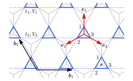
where () creates (annihilates) an electron with spin at the lattice site , and for on the up- (down-) triangles. Here defines the electron occupation number at the lattice site . We are interested in the regime with one electron in each Kagomé lattice unit cell, and thus the electron filling for this Hubbard model is [22, 24]. This model is expected to capture the essential physics of the Mo-based cluster magnets [12, 2]. For the fractional filling here, the Mott localization is driven by the inter-site repulsions () rather than the on-site Hubbard- interaction and the electrons are localized in the (elementary) triangles of the Kagomé lattice instead of the lattice sites. Due to the asymmetry between the up- and down-triangles, the Mott localization in the up-triangles and down-triangles does not occur simultaneously. Setting the Hubbard- as the largest energy scale, we study the properties of the model and explore its phase diagram.
The kinetic part of the model can be readily diagonalized and the electrons form the following three bands,
| (2) | |||||
| (3) |
where , and , are two elementary lattice vectors of the underlying Bravais lattice (see Fig. 1). These three electron bands are well-separated from each other and only touch at certain discrete momentum points. In particular, and have Dirac-point band touchings at the Brillouin zone corners when . With the electron filling, the electrons fill half the lowest band and the ground state of the kinetic part is a Fermi liquid (FL) metal.
III Strong Breathing Limit and Type-I CMI
Electron correlations are considered on top of the kinetic part. A strong Hubbard- merely suppresses double occupation on a single lattice site and cannot cause localization due to the fractional filling here. What replaces is the cluster localization from the inter-site interactions. We first explore the strong breathing limit with and study the cluster localization driven by the remaining interaction in the framework of the slave-rotor construction [28, 29, 30, 31]. A strong repulsion penalizes the double occupancy on the up-triangles and would drive a Mott transition from FL metal to a CMI. Because the number of the up-triangles is equal to the total electron number, there is exactly one electron in each up-triangle in this cluster Mott regime. To describe different phases and study the Mott transitions, we first employ the standard slave-rotor representation for the electron operator , where the bosonic rotor () carries the electron charge and the fermionic spinon () carries the spin quantum number. To constrain the enlarged Hilbert space, we introduce an angular momentum variable ,
| (4) |
where is conjugate to the rotor variable with
| (5) |
Since the interaction is assumed to be the largest, in the large limit the double electron occupation is always suppressed. Hence, the angular variable primarily takes () for a singly-occupied (empty) site. Decoupling the electron hopping into the spinon and the rotor sectors, we obtain the Hamiltonians for the spin and charge sectors
| (6) | |||||
| (7) | |||||
where labels the center of up-triangle or equivalently the unit cell of the lattice,
| (8) | |||||
| (9) |
and is a Lagrangian multiplier to enforce the Hilbert space constraint. The Hamiltonian is invariant under an internal U(1) gauge transformation, , , and . Here we have introduced an angular momentum operator as
| (10) |
where the lattice site is labeled by the combination of the unit cell and the sublattice index . measures the total electron occupation on the up-triangle at . Moreover, from , we find that can take . Finally, because , the last term in the second line of Eq. (7) reduces to a constant and can be dropped. It is convenient to define the conjugate variable for . We introduce a super-rotor operator whose physical meaning is to create and annihilate an electron charge in the up-triangle at . Clearly, we have
| (11) |
As , the hopping terms inside the up-triangles commute with the interaction and we can set . The hopping terms inside the down-triangles, that describe the electron tunneling from the neighboring up-triangles, do not commute with the interaction. Increasing penalizes the kinetic energy gain through hoppings on the down-triangle bonds and causes the electron cluster localization in the up-triangles. Nevertheless, the electrons remain mobile inside each up-triangle and can gain kinetic energy through hoppings within the up-triangle. Thus, the system is locally “metallic” within each up-triangle and remains so even when the interaction becomes dominant.
Using the local metallic condition () to optimize the intra-up-triangle hopping, we obtain a reduced rotor Hamiltonian that is defined on the triangular lattice formed by the centers of the up-triangles,
| (12) | |||||
where labels two neighboring up-triangles and , is defined on down-triangles.
The relevant degrees of freedom for the Mott transition is the super-rotor mode . When it is condensed and , we obtain a FL metal. When it is gapped with , a CMI with electrons localized on all up-triangles is obtained, and we refer this CMI as type-I CMI in Fig. 2(a). In this type-I CMI, there exists charge coherence within the up-triangle as it is “locally metallic”. The gauge field fluctuations within the up-triangles become massive from the Higgs mechanism. The gauge fluctuations on the links between two neighboring up-triangles remain gapless and we represent it by for two up-triangles at and . The reduced rotor Hamiltonian and the spinon Hamiltonian are invariant under the U(1) gauge transformation .
In the type-I CMI, the spinon mean-field Hamiltonian describes the spinon hopping at the mean-field level. The spinon bands are identical to the electronic ones, , except for the modified hopping. Thus, the spinons fill a half of the lowest spinon band, leading to a spinon Fermi surface. The resulting spin sector is a U(1) quantum spin liquid (QSL) with a spinon Fermi surface. It is generally believed that, the U(1) QSL is in the deconfined phase due to the spinon Fermi surface that suppresses the instanton events. When the super-rotor mode is condensed, the U(1) gauge field picks up a mass via the Higgs’ mechanism, and the charge rotor and fermionic spinons are then combined back to the original electron. Here we solve the charge sector Hamiltonian and the spinon Hamiltonian self-consistently for the phase diagram and Mott transition. Following the standard procedure, we implement the coherent state path integral for the super-rotor variables and . By integrating out the field , we obtain the partition function,
| (13) |
with the effective action
| (14) |
We have dropped the term with parameter that is required to vanish since . The Lagrange multiplier is also introduced in the partition function to enforce the unimodular constraint for each up-triangle. We take a uniform saddle point approximation by setting and further integrate out the fields. Finally we get the following saddle point equation in the Mott insulating phase,
| (15) |
where is the area of the first Brillouin zone of the triangular lattice and is the dispersion of the super-rotor mode with
| (16) |
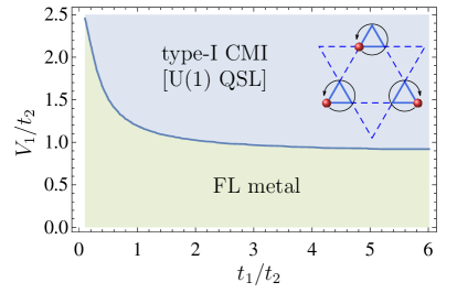
When , the dispersion becomes gapless. That means the super-rotor mode is condensed. Combining this condensation condition with the super-rotor saddle point equation Eq. (15) and the spinon-sector mean-field theory, we construct the phase diagram in the strong breathing limit as shown in Fig. 2(a).
Here we do not consider the possibility of magnetic ordering in the strong Mott regime. For a small (large) , we obtain a Fermi liquid metal (or a U(1) QSL with a spinon Fermi surface). The Mott transition is continuous and of the quantum XY type in the mean-field theory, and is expected to be so even after including the U(1) gauge fluctuations [32]. The phase boundary of the Mott transition is understood as follows. For smaller (larger) , the electrons gain more (less) kinetic energy from the hopping or the inter-up-triangle hopping, and thus, a larger (smaller) critical is needed to localize the electrons in the up-triangles. In particular, in the limit of , our model with and electron filling is equivalent to a triangular lattice Hubbard model at half-filling where the triangular lattice is formed by the up-triangles. Therefore, the U(1) QSL with a Fermi surface in the type-I CMI is smoothly connected to the one proposed for the triangular lattice Hubbard model at half-filling [29, 30].
IV Emergent U(1) gauge structure in type-II CMI
As gradually increases from zero, the free motion of electrons inside the up-triangles becomes less favorable energetically because this motion creates double occupancy configurations on the down-triangles. Thus, at a critical , the electron number on each down-triangle is also fixed to be one, and we experience the cluster localization on both types of triangles. This new cluster Mott state is referred as type-II CMI. The slave-rotor representation in this phase fails to capture the proper physics and we should introduce a new parton construction. Before that, we need to first understand the low-energy physics of the charge sector, especially in the type-II CMI. We will show the charge localization pattern in the type-II CMI leads to an emergent compact U(1) lattice gauge theory description for the charge-sector quantum fluctuations. In the slave-rotor formalism, the charge-sector Hamiltonian with interaction is given by
| (17) | |||||
where we have dropped the interaction term because only gives a constant for the term in the large limit. Up to a mapping from the rotor operators to the spin ladder operators, , this charge sector Hamiltonian is equivalent to a Kagomé lattice spin-1/2 XXZ model in the presence of an external magnetic field. We can recast the charge sector Hamiltonian as
| (18) | |||||
Here the effective spin- ladder operators satisfy
| (19) |
and the effective “magnetic” field reads . The electron filling can be regarded as the total “magnetization” condition , where is the total number of Kagomé lattice sites.
When the inter-site repulsion dominate over the hoppings , the system enters into the type-II CMI phase where the cluster localization appears on both types of triangles. In terms of the effective spin , the electron charge localization condition in the type-II CMI is
| (20) |
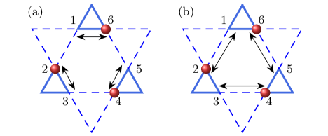
Therefore, the allowed effective spin configuration is “2-down 1-up” in every triangle. These allowed classical spin configurations are extensively degenerate. But the degeneracy will be further lifted after involving the transverse effective spin exchanges. Physically, the effective interactions are originated from the collective hopping processes of electrons (shown in Fig. 3) and can be obtained from a third order degenerate perturbation theory. The resulting ring exchange Hamiltonian has the form of
| (21) |
where “” refers to the elementary hexagon of the Kagomé lattice, is the ring exchange parameter and “1, 2, 3, 4, 5, 6” are the six vertices on the corner of the elementary hexagon on the Kagomé lattice (see Fig. 3).
We now demonstrate that the effective Hamiltonian can be mapped into a compact U(1) lattice gauge theory on the dual honeycomb lattice. As shown in Fig. 1(a), this dual honeycomb lattice is formed by the centers of up- and down- triangles, labeled as and respectively. We follow the previous work Ref. 33 and introduce the lattice U(1) gauge fields () by defining
| (22) | |||||
| (23) |
where , , and . The fields and are identified as the electric field and the vector gauge field of the compact U(1) lattice gauge theory and satisfy . With this identification, the local “2-down 1-up” charge localization condition in Eq. (20) is interpreted as the “Gauss’ law” for the emergent U(1) lattice gauge theory. The effective ring exchange Hamiltonian reduces to a gauge “magnetic” field term on the dual honeycomb lattice,
| (24) |
where is a lattice curl defined on the “” that refers to the elementary hexagon on the dual honeycomb lattice. As this internal gauge structure emerges at the low energies in the charge sector, we refer this gauge field as the U(1) gauge field. The fate of U(1) gauge field can become confining as it is in two spatial dimensions. However, as the gapless spinon matter is involved, it is likely that the instanton events can still get suppressed. Thus, even though the plaquette charge order is expected in previous works [12, 34, 35, 36, 37, 38], the gauge deconfinement can coexist with the charge order. This is very much like the AFM∗ phase where the spin quantum number fractionalization and the antiferromagnetic order coexist [39, 40]. The more detailed structure inside the charge sector of the type-II CMI is not the focus of this work. We are more concerned about the localization pattern and thus assume the charge fractionalization in the type-II CMI. A strict analysis requires non-perturbative computations involving quantum fluctuations and is beyond the mean-field theory. In this work, we ignore the instanton effect and focus on constructing the mean-field phase diagram for the extended Hubbard model.
V Mean-field theory for the transition between type-I to type-II CMIs
In this section, we go beyond the strong breathing limit and build a generic framework which can support both type-I and type-II CMIs. As mentioned in the last section, the slave-rotor representation is incapable of describing the type-II CMI state where cluster localization occurs on both types of triangles. Therefore, we first introduce a new parton representation based on the emergent gauge structure in type-II CMI and then establish the phase diagram at the mean-field level. We also discuss the properties in each clusterization phase and the phase transitions between them.
V.1 Slave-particle Construction and Mean-field Theory
To study the transition between two distinct cluster localization states, we return to the charge sector Hamiltonian in Eq. (7) by adding the interaction,
| (25) | |||||
Since the electron is not localized on a lattice site in the CMIs, the rotor variable is insufficient to describe all the phases and phase transitions, except for the special limits for type-I CMI that we have analyzed. To fix the problem, we extend the slave-rotor representation to a new parton construction for the electron operator [31, 41, 1],
| (26) |
where connects the up-triangle center and the neighboring down-triangle centers , () creates (annihilates) the bosonic charge excitation in the triangle at (), and is an open string operator of the U(1) gauge field in the charge sector connecting the charge excitations in the neighboring triangles at and . Under the U(1) gauge transformation, , and . To constrain the Hilbert space of the parton construction, one defines the following operator [31],
| (27) | |||||
that measures the local U(1) (electric) gauge charge, and for the remaining part of the paper, refers to the centers of both up (denoted as ‘u’) and down (denoted as ‘d’) triangles. Here, () for () and . We further supplement this definition with a Hilbert space constraint [31, 41],
| (28) |
such that the physical Hilbert space is recovered. For the type-II CMI, for every triangle.
Due to the single electron occupancy on all triangles for type-II CMI, the electron motions are correlated in type-II CMI instead of the free electron motion in the inset of Fig. 2(a) for a type-I CMI. This correlated electron motion leads to the emergent U(1) gauge structure here [12] and the plaquette charge order whose consequences on the spin sectors are explained in previous works [12, 34, 35, 36, 37, 38]. This is not the focus of this work where we are more concerned about the distinct types of cluster localization. Using the new parton construction, the Hubbard model becomes
| (29) | |||||
which is supplemented with the Hilbert space constraint. In mean-field treatment, we decouple the kinetic terms and for the charge sector in the up-triangles, for the charge sector in the down-triangles, for the spinon, and for the U(1) gauge link,
where the mean-field parameters are defined by
Here we have dropped the Lagrange multipliers in the decoupled mean field Hamiltonian. Because they arise from the constraints of physical Hilbert space and expected to vanish for the single occupation condition within all triangles in type-II CMI. In the decoupling treatment, we also respect all symmetries of the original Hubbard model to obtain correct mean-field parameters defined above.
V.2 Mean-field Phase Diagram
To solve the bosonic mean-field Hamiltonians, we introduce a rotor variable that is conjugate to the U(1) charge operator with
| (30) |
and hence
| (31) | |||
| (32) |
After carrying out the coherent state path integral for the fields and integrating out the field, the resulting partition functions for the up- and down-triangles share the same form as
| (33) |
where can take ‘u’ (or 1) and ‘d’ (or 2) corresponding to up- and down-triangle subsystems respectively. The Lagrange multiplier is used to implement the unimodular constraint for the field at each site. The effective action for the up- and down-triangle subsystems are
| (34) |
where refers to the nearest-neighbor sites on each type of triangle subsystem. The rest of the treatment on each subsystems is identical to what we did to the super-rotor mode in Sec. III and then we can find the critical at which the bosons are condensed. The resemblance between the above actions and the the action of Eq. (14) indicates the close connection between this slave-particle approach used here and the slave-rotor formulation used in Sec. III. In the strong breathing limit with , this two approaches should give qualitatively the same results. But quantitatively, the current approach, through the string parameters, takes into account of the reduction of the spinon or electron bandwidth due to the on-site Hubbard interaction. As a result, we expect that it could give a more reliable phase diagram especially for the FL metal phase.
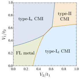
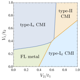
The generic mean-field phase diagrams for different choices of couplings are depicted as Fig. 2(b,c). The four phases correspond to different behaviors of the charge bosons (see Tab. 1). When the charge bosons from both up- and down-triangles are condensed, the FL metal is realized. When they are both gapped and uncondensed, we have the type-II CMI. When the charge bosons from one triangle are condensed and the other is uncondensed, we have the type-I CMI. Here the subindex ‘u’ or ‘d’ to the type-I CMI indicates which triangles the electrons are localized in. In mean-field theory, because the charge is a higher energy degree of freedom, the spinon sector was treated as a spectator, rather than the driving force.
| Type-II CMI | for . |
|---|---|
| Type-I CMI | for , for . |
| Type-I CMI | for , for . |
| FL metal | for , for . |
We turn to explain the phase boundaries in Fig. 2(b,c). As we increase , the effective electron hopping on the up-triangle bonds gets suppressed which effectively enhances the kinetic energy gain through the down-triangle bonds. Thus, a larger is required to drive a Mott transition. A similar argument applies to the boundary between type-I and type-II CMIs. A larger is needed to compete with the kinetic energy gain on the up-triangle bonds for a larger in type-I CMI and to drive a transition to type-II CMI. For , electrons are more likely to be localized in the up-triangles to gain the intra-cluster kinetic energy. Thus, a smaller is needed to drive a Mott transition and a larger is needed to drive the system from type-I to type-II CMIs.
The phase transition between the tpye-I and type-II CMIs can also be understood in the charge boson picture. To be concrete, we focus on the transition from the type-II CMI to the tpye-I CMI and the extension to the tpye-I CMI is direct. In the type-II CMI, charge bosons from both up- and down-triangles are gapped and uncondensed. With the decreasing of the inter-site repulsion on the down-triangle bonds, the charge bosons become condensed on the down-triangle subsystem and the U(1) gauge field also acquires a mass concurrently. The two fractionally-charged charge bosons from two types of triangles then are combined back into the original unit-charged charge rotor . The large inter-site repulsion still preserves the single electron occupancy on the up-triangle subsystem. Thus, the charge rotor is well-defined on the center of an up-triangle and within the up-triangle, the localized electron can move more or less freely. In this sense, the condensation of the charge bosons from the down-triangles leads to the local “metallic” clusters in the up-triangles. After the charge boson condensation, there is no charge fractionalization in the type-I CMI, but the spin-charge separation still survives. Because of the local “metallic” clusters, only the U(1) gauge field living on the down-triangle bonds that connect the up-triangles remains active and continues to fluctuate at the low energies. The low-energy physics is described by the spinon Fermi surface coupled with a fluctuating U(1) gauge field, leading to a U(1) QSL in the triangular lattice formed by the up-triangles.
All transitions discussed above are continuous at mean-field level, except the transition between type-I and type-I CMIs that is strongly first order. Beyond mean-field theory, the transition between FL metal and type-I CMIs will remain continuous and quantum XY type [32, 42] while the transition into type-II CMI may depend on the detailed charge structure inside type-II CMI. Moreover, our mean field theory does not capture the charge quantum fluctuation inside the type-II CMI as described by the compact U(1) gauge theory in Sec. IV, but does obtain qualitatively correct phase boundaries.
VI Discussion
We discuss the experimental relevance and consequences about the Mo-based cluster magnets. These compounds, \ceM2Mo3O8 (M = Mg, Mn, Fe, Co, Ni, Zn, Cd), \ceLiRMo3O8 (R = rare earth) and other related variants [43, 44, 45, 46], incorporate the \ceMo3O13 cluster unit, and the physical properties of most materials have not been carefully studied so far. According to our theory, more anisotropic systems with a stronger breathing tend to favor the type-I CMI. \ceLi2InMo3O8 is more anisotropic than \ceLiZn2Mo3O8 from the lattice parameters. For \ceLiZn2Mo3O8, the spin susceptibility shows a “1/3 anomaly” and double Curie regimes [22, 26]. This was attributed to the plaquette charge order in the type-II CMI that reconstructs the spin sector. In contrast, \ceLi2InMo3O8 is characterized by one Curie regime with the Curie temperature K down to 25K [43]. The Curie constant is consistent with one unpaired spin-1/2 moment per \ceMo3O13 cluster in the type-I CMI. Below 25K, the spin susceptibility of \ceLi2InMo3O8 saturates to a constant, which is consistent with the expectation from a spinon Fermi surface U(1) QSL. Besides the structural and spin susceptibility data, however, very little is known about \ceLi2InMo3O8. It is also likely that this system is located in the 120-degree order state of the model. Thus, more experiments are needed to confirm the absence of magnetic ordering in \ceLi2InMo3O8 and also to explore the magnetic properties of \ceScZnMo3O8 and other cluster magnets [47]. From the numerical aspect, first principal calculation is carried out recently and supports the experimental findings and theoretical understandings in \ceMo3O8 magnets. Namely, \ceLiZn_2Mo3O8 is shown to exhibit the plaquette order with one dangling spin, \ceLi2InMo3O8 is a CMI with 120-degree order and \ceLi2ScMo3O8 displays a spin liquid behavior[48].
Acknowledgements.
We thank the conversation about twisted bilayer graphene with Jianpeng Liu. XQW is supported by MOST 2016YFA0300501, NSFC 11974244, and from a Shanghai talent program. YBK is supported by NSERC of Canada and the Killam Research Fellowship from the Canada Council of the Arts. The remaining authors are supported by the Ministry of Science and Technology of China with Grant No. 2018YFGH000095, 2016YFA0301001, 2016YFA0300500, by Shanghai Municipal Science and Technology Major Project with Grant No.2019SHZDZX04, and by the Research Grants Council of Hong Kong with General Research Fund Grant No.17303819 and No. 17306520.References
- Chen et al. [2014] G. Chen, H.-Y. Kee, and Y. B. Kim, Fractionalized charge excitations in a spin liquid on partially filled pyrochlore lattices, Phys. Rev. Lett. 113, 197202 (2014).
- Chen and Lee [2018] G. Chen and P. A. Lee, Emergent orbitals in the cluster Mott insulator on a breathing kagome lattice, Phys. Rev. B 97, 035124 (2018).
- Carrasquilla et al. [2017] J. Carrasquilla, G. Chen, and R. G. Melko, Tripartite entangled plaquette state in a cluster magnet, Phys. Rev. B 96, 054405 (2017).
- Law and Lee [2017] K. T. Law and P. A. Lee, 1T-TaS2 as a quantum spin liquid, Proc. Natl. Acad. Sci. 114, 6996 (2017).
- He et al. [2018] W.-Y. He, X. Y. Xu, G. Chen, K. T. Law, and P. A. Lee, Spinon fermi surface in a cluster mott insulator model on a triangular lattice and possible application to , Phys. Rev. Lett. 121, 046401 (2018).
- Cao et al. [2018a] Y. Cao, V. Fatemi, A. Demir, S. Fang, S. L. Tomarken, J. Y. Luo, J. D. Sanchez-Yamagishi, K. Watanabe, T. Taniguchi, E. Kaxiras, R. C. Ashoori, and P. Jarillo-Herrero, Correlated insulator behaviour at half-filling in magic-angle graphene superlattices, Nature 556, 80 (2018a).
- Cao et al. [2018b] Y. Cao, V. Fatemi, S. Fang, K. Watanabe, T. Taniguchi, E. Kaxiras, and P. Jarillo-Herrero, Unconventional superconductivity in magic-angle graphene superlattices, Nature 556, 43 (2018b).
- Bistritzer and MacDonald [2011] R. Bistritzer and A. H. MacDonald, Moiré bands in twisted double-layer graphene, Proc. Natl. Acad. Sci. 108, 12233 (2011).
- Xu and Balents [2018] C. Xu and L. Balents, Topological superconductivity in twisted multilayer graphene, Phys. Rev. Lett. 121, 087001 (2018).
- Wu et al. [2019] F. Wu, T. Lovorn, E. Tutuc, I. Martin, and A. H. MacDonald, Topological insulators in twisted transition metal dichalcogenide homobilayers, Phys. Rev. Lett. 122, 086402 (2019).
- Tang et al. [2020] Y. Tang, L. Li, T. Li, Y. Xu, S. Liu, K. Barmak, K. Watanabe, T. Taniguchi, A. H. MacDonald, J. Shan, and K. F. Mak, Simulation of Hubbard model physics in WSe2/WS2 moiré superlattices, Nature 579, 353 (2020).
- Chen et al. [2016] G. Chen, H.-Y. Kee, and Y. B. Kim, Cluster Mott insulators and two Curie-Weiss regimes on an anisotropic kagome lattice, Phys. Rev. B 93, 245134 (2016).
- Lv et al. [2015] J.-P. Lv, G. Chen, Y. Deng, and Z. Y. Meng, Coulomb liquid phases of bosonic cluster mott insulators on a pyrochlore lattice, Phys. Rev. Lett. 115, 037202 (2015).
- Abd-Elmeguid et al. [2004] M. M. Abd-Elmeguid, B. Ni, D. I. Khomskii, R. Pocha, D. Johrendt, X. Wang, and K. Syassen, Transition from mott insulator to superconductor in and under high pressure, Phys. Rev. Lett. 93, 126403 (2004).
- Khomskii and Streltsov [2020] D. I. Khomskii and S. V. Streltsov, Orbital effects in solids: Basics and novel development (2020), arXiv:2006.05920 [cond-mat.str-el] .
- Komleva et al. [2020] E. V. Komleva, D. I. Khomskii, and S. V. Streltsov, Three-site transition-metal clusters: Going from localized electrons to molecular orbitals (2020), arXiv:2007.15230 [cond-mat.str-el] .
- Hirai et al. [2013] D. Hirai, M. Bremholm, J. M. Allred, J. Krizan, L. M. Schoop, Q. Huang, J. Tao, and R. J. Cava, Spontaneous formation of zigzag chains at the metal-insulator transition in the -pyrochlore , Phys. Rev. Lett. 110, 166402 (2013).
- Streltsov and Khomskii [2018] S. V. Streltsov and D. I. Khomskii, Cluster magnetism of Ba4NbMn3O12: Localized electrons or molecular orbitals?, JETP Lett. 108, 686–690 (2018).
- Kim et al. [2014] H.-S. Kim, J. Im, M. J. Han, and H. Jin, Spin-orbital entangled molecular states in lacunar spinel compounds, Nat. Commun. 5, 3988 (2014).
- Streltsov et al. [2017] S. V. Streltsov, G. Cao, and D. I. Khomskii, Suppression of magnetism in : Interplay of Hund’s coupling, molecular orbitals, and spin-orbit interaction, Phys. Rev. B 96, 014434 (2017).
- Radaelli et al. [2002] P. G. Radaelli, Y. Horibe, M. J. Gutmann, H. Ishibashi, C. H. Chen, R. M. Ibberson, Y. Koyama, Y.-S. Hor, V. Kiryukhin, and S.-W. Cheong, Formation of isomorphic Ir3+ and Ir4+ octamers and spin dimerization in the spinel CuIr2S4, Nature 416, 155 (2002).
- Sheckelton et al. [2012] J. P. Sheckelton, J. R. Neilson, D. G. Soltan, and T. M. McQueen, Possible valence-bond condensation in the frustrated cluster magnet LiZn2Mo3O8, Nat. Mater. 11, 493 (2012).
- Mourigal et al. [2014] M. Mourigal, W. T. Fuhrman, J. P. Sheckelton, A. Wartelle, J. A. Rodriguez-Rivera, D. L. Abernathy, T. M. McQueen, and C. L. Broholm, Molecular quantum magnetism in , Phys. Rev. Lett. 112, 027202 (2014).
- Akbari-Sharbaf et al. [2018] A. Akbari-Sharbaf, R. Sinclair, A. Verrier, D. Ziat, H. D. Zhou, X. F. Sun, and J. A. Quilliam, Tunable quantum spin liquidity in the th-filled breathing kagome lattice, Phys. Rev. Lett. 120, 227201 (2018).
- Sheckelton et al. [2015] J. P. Sheckelton, J. R. Neilson, and T. M. McQueen, Electronic tunability of the frustrated triangular-lattice cluster magnet LiZn2-xMo3O8, Mater. Horiz. 2, 76 (2015).
- Sheckelton et al. [2014] J. P. Sheckelton, F. R. Foronda, L. Pan, C. Moir, R. D. McDonald, T. Lancaster, P. J. Baker, N. P. Armitage, T. Imai, S. J. Blundell, and T. M. McQueen, Local magnetism and spin correlations in the geometrically frustrated cluster magnet , Phys. Rev. B 89, 064407 (2014).
- Li and Wang [2009] C. Li and Z. Wang, Mott and Wigner-Mott transitions in doped correlated electron systems: Effects of superlattice potential and intersite correlation, Phys. Rev. B 80, 125130 (2009).
- Florens and Georges [2004] S. Florens and A. Georges, Slave-rotor mean-field theories of strongly correlated systems and the Mott transition in finite dimensions, Phys. Rev. B 70, 035114 (2004).
- Lee and Lee [2005a] S.-S. Lee and P. A. Lee, U(1) gauge theory of the Hubbard model: Spin liquid states and possible application to , Phys. Rev. Lett. 95, 036403 (2005a).
- Lee and Lee [2005b] S.-S. Lee and P. A. Lee, Emergent U(1) gauge theory with fractionalized boson/fermion from the Bose condensation of excitons in a multiband insulator, Phys. Rev. B 72, 235104 (2005b).
- Lee et al. [2012] S. Lee, S. Onoda, and L. Balents, Generic quantum spin ice, Phys. Rev. B 86, 104412 (2012).
- Senthil [2008a] T. Senthil, Theory of a continuous Mott transition in two dimensions, Phys. Rev. B 78, 045109 (2008a).
- Hermele et al. [2004] M. Hermele, M. P. A. Fisher, and L. Balents, Pyrochlore photons: The spin liquid in a three-dimensional frustrated magnet, Phys. Rev. B 69, 064404 (2004).
- Pollmann et al. [2008] F. Pollmann, P. Fulde, and K. Shtengel, Kinetic ferromagnetism on a kagome lattice, Phys. Rev. Lett. 100, 136404 (2008).
- Banerjee et al. [2008] A. Banerjee, S. V. Isakov, K. Damle, and Y. B. Kim, Unusual liquid state of hard-core bosons on the pyrochlore lattice, Phys. Rev. Lett. 100, 047208 (2008).
- Rüegg and Fiete [2011] A. Rüegg and G. A. Fiete, Fractionally charged topological point defects on the kagome lattice, Phys. Rev. B 83, 165118 (2011).
- Ferhat and Ralko [2014] K. Ferhat and A. Ralko, Phase diagram of the -filled extended Hubbard model on the kagome lattice, Phys. Rev. B 89, 155141 (2014).
- Pollmann et al. [2014] F. Pollmann, K. Roychowdhury, C. Hotta, and K. Penc, Interplay of charge and spin fluctuations of strongly interacting electrons on the kagome lattice, Phys. Rev. B 90, 035118 (2014).
- Lannert and Fisher [2003] C. Lannert and M. P. A. Fisher, Inelastic neutron scattering signal from deconfined spinons in a fractionalized antiferromagnet, Int. J. Mod. Phys. B 17, 2821–2838 (2003).
- Lannert et al. [2001] C. Lannert, M. P. A. Fisher, and T. Senthil, Electron spectral function in two-dimensional fractionalized phases, Phys. Rev. B 64, 014518 (2001).
- Savary and Balents [2012] L. Savary and L. Balents, Coulombic quantum liquids in spin- pyrochlores, Phys. Rev. Lett. 108, 037202 (2012).
- Senthil [2008b] T. Senthil, Critical Fermi surfaces and non-Fermi liquid metals, Phys. Rev. B 78, 035103 (2008b).
- Gall et al. [2013] P. Gall, R. A. R. A. Orabi, T. Guizouarn, and P. Gougeon, Synthesis, crystal structure and magnetic properties of Li2InMo3O8: A novel reduced molybdenum oxide containing magnetic Mo3 clusters, J. Solid State Chem. 208, 99 (2013).
- McCarroll et al. [1957] W. H. McCarroll, L. Katz, and R. Ward, Some ternary oxides of tetravalent molybdenum, J. Am. Chem. Soc. 79, 5410 (1957).
- Torardi and McCarley [1985] C. C. Torardi and R. E. McCarley, Synthesis, crystal structures, and properties of lithium zinc molybdenum oxide (LiZn2Mo3O8), zinc molybdenum oxide (Zn3Mo3O8), and scandium zinc molybdenum oxide (ScZnMo3O8), reduced derivatives containing the Mo3O13 cluster unit, Inorg. Chem. 24, 476 (1985).
- McCarroll [1977] W. H. McCarroll, Structural relationships in ARMo3O8 metal atom cluster oxides, Inorg. Chem. 16, 3351 (1977).
- Haraguchi et al. [2015] Y. Haraguchi, C. Michioka, M. Imai, H. Ueda, and K. Yoshimura, Spin-liquid behavior in the spin-frustrated cluster magnet in contrast to magnetic ordering in isomorphic , Phys. Rev. B 92, 014409 (2015).
- Nikolaev et al. [2020] S. A. Nikolaev, I. V. Solovyev, and S. V. Streltsov, Quantum spin liquid and cluster mott insulator phases in the Mo3O8 magnets (2020), arXiv:2001.07471 [cond-mat.str-el] .