FederBoost: Private Federated Learning for GBDT

Abstract

Federated Learning (FL) has been an emerging trend in machine learning and artificial intelligence. It allows multiple participants to collaboratively train a better global model and offers a privacy-aware paradigm for model training since it does not require participants to release their original training data. However, existing FL solutions for vertically partitioned data or decision trees require heavy cryptographic operations.

In this paper, we propose a framework named FederBoost for private federated learning of gradient boosting decision trees (GBDT). It supports running GBDT over both vertically and horizontally partitioned data. Vertical FederBoost does not require any cryptographic operation and horizontal FederBoost only requires lightweight secure aggregation. The key observation is that the whole training process of GBDT relies on the ordering of the data instead of the values.

We fully implement FederBoost and evaluate its utility and efficiency through extensive experiments performed on three public datasets. Our experimental results show that both vertical and horizontal FederBoost achieve the same level of accuracy with centralized training where all data are collected in a central server; and they are 4-5 orders of magnitude faster than the state-of-the-art solutions for federated decision tree training; hence offering practical solutions for industrial application.

1 Introduction

It is commonly known that big data plays an essential role in machine learning. Such big data are typically pooled together from multiple data sources and processed by a central server (i.e., centralized learning). Now, it becomes troublesome to conduct such activities as the governments are increasingly concerned with unlawful use and exploitation of users’ personal data. For example, the European Union has recently enacted General Data Protection Regulation (GDPR), which was designed to give users more control over their data and impose stiff fines on enterprises for non-compliance. Consequently, service providers become unwilling to take the risk of potential data breaches and centralized learning becomes undesirable.

Federated learning (FL) [1] addresses this challenge by following the idea of transferring intermediate results of the training algorithm instead of the data itself. More specifically, it offers a privacy-aware paradigm of model training which does not require data sharing, but allows participants to collaboratively train a more accurate global model. Since 2017 when it was first proposed by Google [1], significant efforts have been put by both researchers and practitioners to improve FL [2, 3, 4, 5, 6, 7, 8]. Nevertheless, there are still two problems remain unsolved by the community: (1) unable to efficiently handle vertically partitioned data, and (2) unable to efficiently support decision trees.

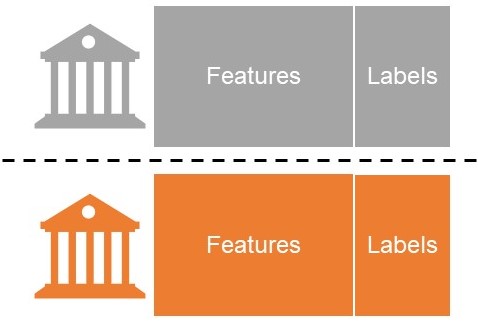
(a) Horizontally partitioned data.

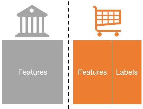
(b) Vertical partitioned data.

Figure 1: Data partitions for federated learning.

Horizontal and Vertical FL. Base on how data is partitioned, FL can be roughly classified into two categories: horizontal FL and vertical FL [9]. Horizontal FL, also known as sample-wise FL, targets the scenarios where participants’ data have the same feature space but differ in samples (cf. Figure 1(a)). For example, two regional banks might have the same feature space as they are running the same business; whereas the intersection of their samples is likely to be small since they serve different customers in their respective regions. Vertical FL or feature-wise FL targets the scenarios where participants’ data have the same sample space but differ in features (cf. Figure 1(b)). For example, consider two participants, one is a bank and the other is an e-commerce company. They can find a large intersection between their respective sample spaces, because a customer needs a bank account to use the e-commerce service. Their feature spaces are certainly different as they are running different businesses: the bank records users’ revenue, expenditure behavior and credit rating, and the e-commerce company retains users’ browsing and purchasing history. Unlike horizontal FL that has been extensively studied by the research committee, less attention has been paid to vertical FL. Existing vertical FL schemes rely on heavy cryptographic technologies such as homomorphic encryption and secure multiparty computation to combine the feature space of multiple participants [10, 9, 11, 12].

Decision trees. The FL research committee is focusing on neural networks and pays less attention to other machine learning models such as decision trees. Even though neural networks are the most prevailing models in academia, they are notorious for a lack of interpretability, which hinders their adoptions in some real-world scenarios like finance and medical imaging. In contrast, decision tree is considered as a gold standard for accuracy and interpretability. A decision tree outputs a sequence of decisions leading to the final prediction, and these intermediate decisions can be verified and challenged separately. Additionally, gradient boosting decision tree (GBDT) such as XGBoost [13] is regard as a standard recipe for winning ML competitions. Unfortunately, decision trees have not received enough attentions in FL research. To the best of our knowledge, most privacy-preserving FL frameworks for decision trees are fully based on cryptographic operations [14, 15, 16, 17] and they are expensive to be deployed in practice. For example, the state-of-the-art solution [16] takes $\sim$28 hours to train a GBDT in LAN from a dataset that consists of 8 192 samples and 11 features.

Our contribution. In this paper, we propose a novel framework named FederBoost for private federated learning of decision trees. It supports running GBDT over both horizontally and vertically partitioned data.

The key observation for designing FederBoost is that the whole training process of GBDT relies on the ordering of the samples in terms of their relative magnitudes. Therefore, in vertical FederBoost, it is enough to have the participant holding the labels collect the ordering of samples from other participants; then it can run the GBDT training algorithm in exactly the same way as centralized learning. We further utilize bucketization and differential privacy (DP) to protect the ordering of samples: participants partition the sorted samples of a feature into buckets, which only reveals the ordering of the buckets; we also add differentially private noise to each bucket. Consequently, vertical FederBoost achieves privacy without using any cryptographic operations.

The case for horizontally partitioned data is tricky, since the samples and labels are distributed among all participants: no one knows the ordering of samples for a feature. To conquer this, we propose a novel method for distributed bucket construction so that participants can construct the same global buckets as vertical FederBoost even though the samples are distributed. We also use secure aggregation [18] to compute the gradients for each bucket given that no single party holds the labels. Both the bucket construction method and secure aggregation are lightweight, hence horizontal FederBoost is as efficient as the vertical one.

We summarize our main contribution as follows:

• We propose FederBoost: a private federated learning framework for GBDT. It supports both horizontally and vertically partitioned data.

• In vertical FederBoost, we define a new variant of DP, which is more friendly for high-dimensional data and saves much privacy budget in a vertical setting.

• In horizontal FederBoost, we propose a novel method for distributed bucket construction.

• We evaluate the utility of FederBoost on three public datasets. The results show that it achieves the same level of accuracy with centralized learning.

• We provide a full implementation of FederBoost and deploy it on a cluster of upto 32 nodes. The benchmark results show that both vertical and horizontal FederBoost are 4-5 orders of magnitude faster than the state-of-the-art solutions [16, 17] for federated decision tree training.

2 Preliminaries

This section provides necessary background and preliminaries for understanding this paper.

2.1 Gradient boosting decision tree (GBDT)

A decision tree is a tree-like model for machine learning predictions. It consists of nodes and edges: each internal node represents a “test” on a feature; each edge represents the outcome of the test; and each leaf node represents the prediction result. The path from root to a leaf represents a prediction rule.

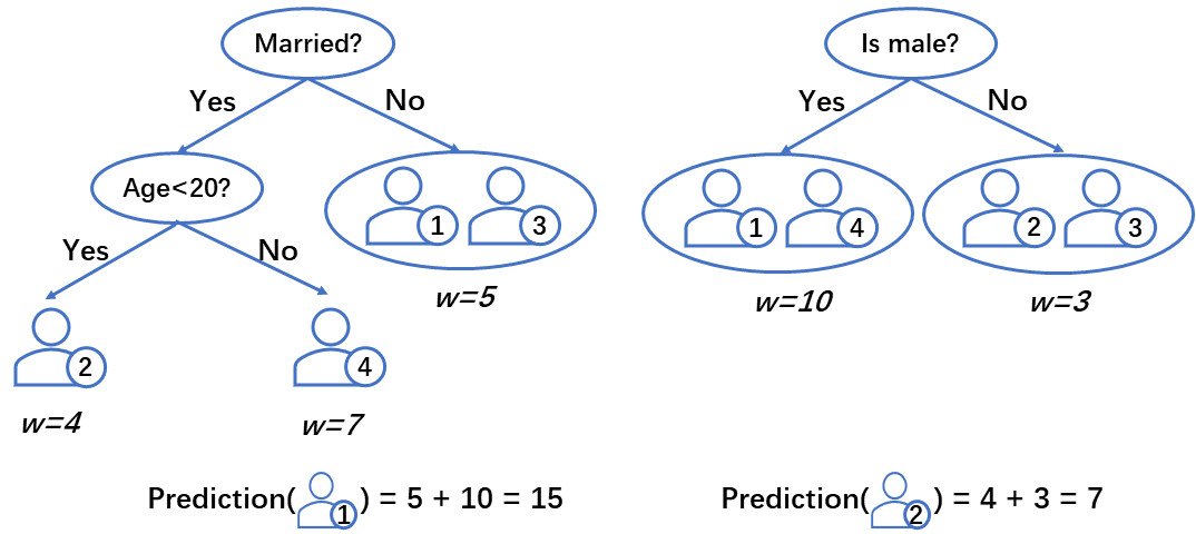
Figure 2: An example of GBDT.

Gradient boosting decision tree (GBDT) is a boosting-based machine learning algorithm that ensembles a set of decision trees [13]. Figure 2 shows an example of GBDT: in each tree, the input ${\mathbf{x}}$ is classified to one leaf node that predicts the input with a weight; then it sums the predictions of all trees and gets the final prediction:

$$\hat{y}=\sum_{t=1}^{T}f_{t}({\mathbf{x}})$$ (1)

where $T$ denotes the number of trained decision trees and $f_{t}({\mathbf{x}})$ denotes the prediction result of the $t$th tree. For classification, it calculates $p=\mathrm{sigmoid}(\hat{y})$ and determines its predicted class based on $p$.

Next, we explain how a GBDT training algorithm works given a dataset $\textbf{X}\in\mathbb{R}^{n\times m}$ that consists of $n$ samples and $m$ features. It first initializes the prediction result $\hat{y}^{0}_{i}$ for each sample with random values. Then, it trains the $t$th decision tree as follows:

1. For each sample, calculate the first- and second-order gradient:

   $$\begin{split}g_{i}=\partial_{\hat{y_{i}}^{(t-1)}}L(y_{i},\hat{y_{i}}^{(t-1)}),\\ h_{i}=\partial^{2}_{\hat{y_{i}}^{(t-1)}}L(y_{i},\hat{y_{i}}^{(t-1)})\end{split}$$ (2)

   where $\hat{y_{i}}^{(t-1)}$ is the prediction result aggregated from previous trees, $y_{i}$ is the real label, and $L(y_{i},\hat{y_{i}}^{(t-1)})$ is the loss function. The binary cross entropy loss function is typically used as a loss function.

2. Run the following steps for each node of the tree from root to leaf:

   1. For each feature, find the best split of the samples that maximize the following function:

      $$\mathcal{L_{\mathit{split}}}= \frac{1}{2}[\frac{(\sum_{i\in I_{L}}g_{i})^{2}}{\sum_{i\in I_{L}}h_{i}+\lambda}$$ (3)

      $$+ \frac{(\sum_{i\in I_{R}}g_{i})^{2}}{\sum_{i\in I_{R}}h_{i}+\lambda}+\frac{(\sum_{i\in I}g_{i})^{2}}{\sum_{i\in I}h_{i}+\lambda}]$$

      where $\lambda$ is a hyper-parameter, $I_{L}$ denotes the samples divided into the left child node, $I_{R}$ denotes the samples divided into the right child node, and $I$ denotes all samples in the current node. The samples in $I_{L}$, $I_{R}$ and $I$ are in a sorted order of their corresponding feature values.

   2. Choose the feature with the maximal $\mathcal{L_{\mathit{split}}}$ for the current node and split the samples accordingly.

3. The weight of each leaf is computed by the following function:

   $$w=-\frac{\sum_{i\in I}g_{i}}{\sum_{i\in I}h_{i}+\lambda}$$ (4)

   This is the prediction result for the samples falling into this leaf.

Most GBDT frameworks accelerate the training process by building a gradient histogram for each feature to summarize the gradient statistics; the best split can be found based on the histograms. More specifically, for each feature, the training algorithm sorts the samples based on their feature values as before. Then, it partitions the samples and puts them into $q$ buckets. For each bucket, it calculates $G=\sum_{i\in\mathit{bucket}}g_{i}$ and $H=\sum_{i\in\mathit{bucket}}h_{i}$. The gradient histogram for a feature consists of these $G$s and $H$s of all buckets. Then, the best split for a feature can be found by maximizing:

$$\mathcal{L_{\mathit{split}}}=\frac{1}{2}[\frac{(\sum_{i\in I_{L}}G_{i})^{2}}{\sum_{i\in I_{L}}H_{i}+\lambda}+\frac{(\sum_{i\in I_{R}}G_{i})^{2}}{\sum_{i\in I_{R}}H_{i}+\lambda}+\frac{(\sum_{i\in I}G_{i})^{2}}{\sum_{i\in I}H_{i}+\lambda}]$$ (5)

Empirically, 20 buckets are used in popular GBDT frameworks [19, 20]. The split finding algorithm is depicted in Algorithm 1.

Input: $\{G_{1},...,G_{q}\}$, $\{H_{1},...,H_{q}\}$

Output: split with max score

1 ${\mathsf{G}}\leftarrow\sum_{i=1}^{q}G_{i}$, ${\mathsf{H}}\leftarrow\sum_{i=1}^{q}H_{i}$

2${\mathsf{G}}_{L}\leftarrow 0$, ${\mathsf{G}}_{R}\leftarrow 0$

3for $i=1\to q$ do

4       ${\mathsf{G}}_{L}\leftarrow{\mathsf{G}}_{L}+G_{i}$, ${\mathsf{H}}_{L}\leftarrow{\mathsf{H}}_{L}+H_{i}$

5      ${\mathsf{G}}_{R}\leftarrow{\mathsf{G}}-{\mathsf{G}}_{L}$, ${\mathsf{H}}_{R}\leftarrow{\mathsf{H}}-{\mathsf{H}}_{L}$

6      $\mathit{score}\leftarrow max(\mathit{score},\frac{G_{L}^{2}}{H_{L}+\lambda}+\frac{G_{R}^{2}}{H_{R}+\lambda}+\frac{G^{2}}{H+\lambda})$

7 end for

Algorithm 1 Split Finding

2.2 Federated learning

The goal of federated learning (FL) is to enable multiple participants to contribute various training data to train a better model. It can be roughly classified into two categories [9]: horizontal FL and vertical FL.

One horizontal FL method [1] proposed by Google is to distribute the model training process of a deep neural network across multiple participants by iteratively aggregating the locally trained models into a joint global one. There are two types of roles in this protocol: a parameter server and $l$ participants $\mathcal{P}$s. In the beginning, the parameter server initializes a model with random values and sends it to all $\mathcal{P}$s. In each iteration, each $\mathcal{P}_{j}$ ($j\in[1,l]$) trains the received model with its local data, and sends parameter server its gradients. The parameter server aggregates the received gradients and updates the global model.

This elegant paradigm cannot be directly applied to vertical FL, where participants have different feature spaces so that they cannot train models locally. Furthermore, the FL research committee is focusing on neural networks and less attention has been paid to decision trees.

2.3 Secure aggregation

Bonawitz, et al. [18] propose a secure aggregation protocol to protect the local gradients in Google’s horizontal FL. Specifically, they use pairwise additive masking to protect participants’ local gradients, and have the parameter server aggregate the masked inputs. The masks are generated by a pseudorandom generator (PRG) using pairwise shared seeds and will get canceled after aggregation. The seeds are shared via threshold secret sharing so that dropped-out participants can be handled. A malicious server can lie about whether a $\mathcal{P}_{i}$ has dropped out, thereby asking all other participants to reveal their shares of $\mathcal{P}_{i}$’s masks. To solve this issue, they introduce a double masking scheme requiring each participant to add another mask to its input and share this mask as well. The server can request either a share of the pairwise mask (which will get canceled if no one drops) or a share of the new mask; an honest participant will never reveal both shares for the same participant to the server. In this paper, we assume the participants are large organisations and they will not drop out in the middle of the protocol, thereby we significantly simplify the secure aggregation protocol.

2.4 Differential privacy

Given a set of input data and an analysis task to perform, the goal of differential privacy [21] is to permit statistical analysis while protecting each individual’s data. It aims to “hide” some input data from the output: by looking at the statistical results calculated from the input data, one cannot tell whether the input data contains a certain record or not.

Definition 2.1 ($\varepsilon$-Differential Privacy [21]).

A randomized algorithm $\mathcal{M}$ with domain $\mathbb{N}^{|\mathcal{X}|}$ is $\varepsilon,$-differentially private if for all $\mathcal{S}\subseteq\mathtt{Range}\left(\mathcal{M}\right)$ and for any neighboring datasets $D$ and $D^{\prime}$:

$$\Pr[\mathcal{M}(D)\in\mathcal{S}]\leq e^{\varepsilon}\Pr[\mathcal{M}(D^{\prime})\in\mathcal{S}].$$

It guarantees that, by examining the outputs $\mathcal{M}(D)$ and $\mathcal{M}(D^{\prime})$, one cannot reveal the difference between $D$ and $D^{\prime}$. Clearly, the closer $\epsilon$ is to $0$, the more indistinguishable $\mathcal{M}(D)$ and $\mathcal{M}(D^{\prime})$ are, and hence the better the privacy guarantee. This nice property provides plausible deniability to the data owner, because the data is processed behind a veil of uncertainty.

3 Problem Statement

We consider the setting of $l$ participants $\mathcal{P}_{1},...,\mathcal{P}_{l}$, holding datasets ${\mathbf{X}}_{1},...,{\mathbf{X}}_{l}$ respectively, want to jointly train a model. We consider both vertically (Section 4) and horizontally (Section 5) partitioned data. We assume there is a secure channel between any two participants, hence it is private against outsiders. The participants are incentivized to train a good model (they will not drop out in the middle of the protocol), but they want to snoop on others’ data. We do not assume any threshold on the number of compromised participants, i.e., from a single participant’s point of view, all other participants can be compromised.

Poisoning attacks and information leakage from the trained model are not considered in this work. We remark that information leakage from the trained model should be prevented when we consider to publish the model. This requires differentially private training [22, 23], which guarantees that one cannot infer any membership about the training data from the trained model. However, this line of research is orthogonal to federated learning (which aims to achieve collaborative learning while keeping the training data local), and we leave it as future work to include it into our protocol.

Given the above setting, we aim to propose FL schemes with the following design goals:

• The efficiency should be close to the traditional distributed ML [13, 20, 19, 24], i.e., the number of cryptographic operations should be minimized.

• The accuracy should be close to the centralized learning, which is to pool all data into a centralized server.

• The privacy should be close to the local training, i.e., each participant trains with its local data only. To achieve this, all data being transferred should be protected either by cryptographic technology or differential privacy.

Lastly, frequently used notations are summarized in Table I.

TABLE I: Summary of notations

Notation	Description
$\mathcal{P}$	participant
$l$	number of participants
$\tau$	number of compromised participants
$n$	number of samples
$m$	number of features
$q$	number of buckets
$T$	number of decision trees
${\mathbf{X}}$	dataset
${\mathbf{x}}^{i}$	$i$th feature
${\mathbf{x}}_{j}$	$j$th sample
$x^{i}_{j}$	value of $i$th feature $j$th sample
$y$	label
$\hat{y}$	prediction result
$g_{i}$, $h_{i}$	first and second order gradient
$Q$	quantile
$\epsilon$	level of differential privacy

4 Vertical FederBoost

In vertical FL, $l$ participants $\mathcal{P}_{1},...,\mathcal{P}_{l}$, holding feature sets ${\mathbf{X}}_{1},...,{\mathbf{X}}_{l}$ respectively, want to jointly train a model. Only a single participant (e.g., $\mathcal{P}_{l}$) holds the labels ${\mathbf{y}}$. Each feature sets ${\mathbf{X}}_{i}$ consists of a set of features: ${\mathbf{X}}_{i}=\left[{\mathbf{x}}^{j},...,{\mathbf{x}}^{k}\right]$ and there are $m$ features in total. Each ${\mathbf{x}}^{i}$ consists all $n$ samples:

${\mathbf{x}}^{i}=\left[x^{i}_{1},x^{i}_{2},...,x^{i}_{n}\right]^{\top}$; similarly, ${\mathbf{y}}=\left[y_{1},y_{2},...,y_{n}\right]^{\top}$ We assume that the secure record linkage procedure has been done already, i.e., all $l$ participants know that their commonly held samples are ${\mathbf{x}}_{1}...{\mathbf{x}}_{n}$. We remark that this procedure can be done privately via multi-party private set intersection [25], which is orthogonal to our paper.

4.1 Training

Input: each $\mathcal{P}_{i}$ inputs feature ${\mathbf{x}}^{i}=\{x^{i}_{1},...,x^{i}_{n}\}$ for simplicity, we assume each $\mathcal{P}_{i}$ holds a single feature, hence $m=l$

Input: $\mathcal{P}_{l}$ inputs labels ${\mathbf{y}}=\{y_{1},...,y_{n}\}$

Output: $T$ decision trees

1

2for $i=1\to l$ do for each $\mathcal{P}$

3       $\mathcal{P}_{i}$ sorts ${\mathbf{x}}^{i}$ and partitions it into $q$ buckets

4      for $j=1\to n$ do for each sample

5             $\mathcal{P}_{i}$ moves $x^{i}_{j}$ to another bucket with probability $\frac{q-1}{e^{\varepsilon}+q-1}$ add DP noise

6       end for

7      $\mathcal{P}_{i}$ sends sample IDs in each bucket to $\mathcal{P}_{l}$

8 end for

9

10$\mathcal{P}_{l}$ initializes $\{\hat{y}_{1},...,\hat{y}_{n}\}$ with random values

11for $t=1\to T$ do for each tree

12       for $i=1\to n$ do for each sample

13             $\mathcal{P}_{l}$: $g_{i}\leftarrow\partial_{\hat{y_{i}}}L(y_{i},\hat{y_{i}})$, $h_{i}\leftarrow\partial^{2}_{\hat{y_{i}}}L(y_{i},\hat{y_{i}})$

14       end for

15      

16      for each node in the current tree do

17            

18            for $i=1\to m$ do for each feature

19                   for $j=1\to q$ do for each bucket

20                        

21                        $\mathcal{P}_{l}$ updates $\mathit{bucket}^{i}_{j}$ not for root

22                        $\mathcal{P}_{l}$: $G^{i}_{j}\leftarrow\sum_{k\in\mathit{bucket}^{i}_{j}}g^{i}_{j,k}$ $H^{i}_{j}\leftarrow\sum_{k\in\mathit{bucket}^{i}_{j}}h^{i}_{j,k}$

23                   end for

24                  $\mathit{score}_{i}$, $\mathit{split}_{i}$ $\leftarrow\mathcal{P}_{l}$ runs Algorithm 1 with inputs $\{G^{i}_{1},...,G^{i}_{q}\}$, $\{H^{i}_{1},...,H^{i}_{q}\}$

25             end for

26            for the maximal $\mathit{score}_{j}$, $\mathcal{P}_{l}$ sends $\mathit{split}_{j}$ to $\mathcal{P}_{j}$ $\mathcal{P}_{l}$ splits the buckets based on $\mathit{split}_{j}$

27       end for

28      $\mathcal{P}_{l}$ updates $\{\hat{y}_{1},...,\hat{y}_{n}\}$ based on the weights (cf. equation 4) of the leaf nodes.

29 end for

Protocol 2 Vertical FederBoost

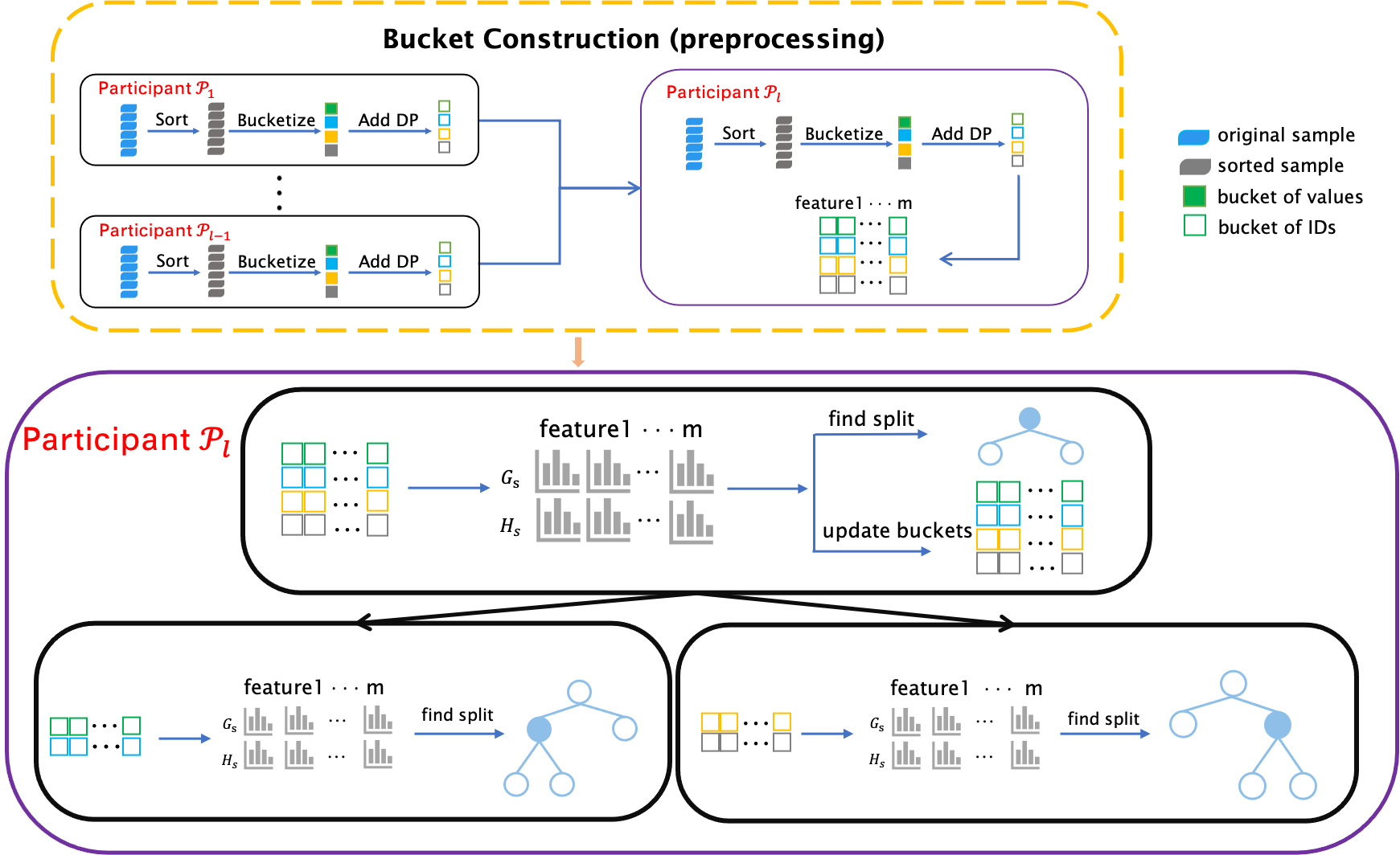
Figure 3: Vertical FederBoost

Vertical FederBoost is based on the observation that the whole training process of GBDT does not involve feature values (cf. Section 2.1). Recall that the crucial step for building a decision tree is to find the best split of samples for a feature, which only requires the knowledge of the first- and second- order gradients $g_{i}$s, $h_{i}$s, as well as the order of samples (Equation 3). Furthermore, $g_{i}$s and $h_{i}$s are calculated based on the labels and the prediction results of previous tree (equation 2). Therefore, to train a GBDT model, only the labels (held by $\mathcal{P}_{l}$), the prediction results of the previous tree, and the order of samples are required.

To this end, we let each participant sort its feature samples and tell $\mathcal{P}_{l}$ the order. With these information, $\mathcal{P}_{l}$ can complete the whole training process by itself. In this way, participants only need to transfer sample orders instead of values, which reveal much less information. Another advantage of this method is that the sorting information only needs to be transferred once, and $\mathcal{P}_{l}$ can use it to fine-tune the model without further communication.

However, information leakage from the sample orders is still significant. Take a feature “salary” as an example, $\mathcal{P}_{l}$ can get such information: “Alice’s salary $\leq$ Bob’s salary $\leq$ Charly’s salary”. If $\mathcal{P}_{l}$ knows Alice’s salary and Charly’s salary, it can infer Bob’s salary (or at least the range). We combine two methods to prevent such information leakage: putting samples into buckets and adding differentially private noise (cf. Section 2.4).

In more detail, for each feature, $\mathcal{P}_{i}$ sorts the samples based on their feature values, partitions the samples and puts them into $q$ buckets. In this way, $\mathcal{P}_{l}$ only knows the order of the buckets but learns nothing about the order of the samples inside a bucket. To further protect the order of two samples in different buckets, we add differentially private noise to each bucket. That is, for a sample that was originally assigned to the $i$th bucket:

• with probability $p=\frac{e^{\varepsilon}}{e^{\varepsilon}+q-1}$, it stays in the $i$th bucket;

• with probability $p^{\prime}=\frac{1}{e^{\varepsilon}+q-1}$, it moves to the $j$th bucket that is picked uniformly at random.

This mechanism is similar to random response [26], which achieves $\epsilon$-LDP. Let $\mathsf{bucketize}(x)$ denote the bucketization mechanism mentioned above and its output is the bucket ID. Then, for any two samples $x_{1}$, $x_{2}$ and a bucket $B$, we have $\forall k\in\{1,...,q\}$:

$$\frac{Pr\left[\mathsf{bucketize}(x_{1})=k\right]}{Pr\left[\mathsf{bucketize}(x_{2})=k\right]}\leq \frac{p}{p^{\prime}}= \frac{e^{\varepsilon}/(e^{\varepsilon}+q-1)}{1/(e^{\varepsilon}+q-1)}$$

$$= e^{\varepsilon},$$

where $Pr\left[\mathsf{bucketize}(x)=k\right]$ denotes the probability that a sample $x$ is placed in bucket $B_{k}$. We present the security analysis of the mechanism in Section 4.2.

Our experimental results (cf. Section 6.1) show that, when $\epsilon=4$ and $q=16$, the accuracy achieved by vertical FederBoost is very close to that without DP. On the other hand, with this configuration, each sample has probability of approximately 22% to be placed in a wrong bucket.

The whole training process for vertical FederBoost is depicted in Protocol 2, and we separately detail the security analysis from the perspective of $\mathcal{P}_{i}$ and $\mathcal{P}_{l}$ in Section 4.3. The passive participants $\mathcal{P}_{1}...\mathcal{P}_{l-1}$ first locally build their buckets and send the sample IDs in each bucket to the active participant $\mathcal{P}_{l}$ (line 1 - 7). We remark that this process only needs to be done once, and $\mathcal{P}_{l}$ can use these buckets to fine-tune the model (i.e., train a model many times with different hyper-parameters).

Then, $\mathcal{P}_{l}$ runs the training algorithm in exactly the same way as centralized GBDT described in Section 2.1 (line 8-24). It first calculates the first- and second- order gradients for each sample (line 10-12). Notice that these gradients need to be updated when a new tree is initialized, based on the prediction results $\{\hat{y}_{1},...,\hat{y}_{n}\}$ of the previous tree. For each node of a tree, $\mathcal{P}_{l}$ needs to find the best split for every feature and choose the best feature (line 14-20). To do this, it builds the gradients histograms for each feature (line 15-18). The sample IDs in each bucket need to be updated for a non-root node (line 16), because the samples got split when its parent-node was built (line 19). After finding the best feature, $\mathcal{P}_{l}$ tells the participant $\mathcal{P}_{j}$ holding this feature how the samples is split (line 21). Figure 3 visualizes the whole training process of vertical FederBoost.

4.2 Element-Level Local DP

Differential privacy (DP), as well as local differential privacy, provides strong protections against attackers, and guarantees that one cannot tell whether a particular sample is in the database or not. However, this kind of strong protection are not necessary in vertical FL, as participants need to know their commonly held samples to run the protocol. In other words, protecting the privacy of data generated by one individual instead of protecting whether one generates private data or not is much more significant. For instance, an online shopping user shopping on the internet many times. In such cases, it may be satisfying from a privacy perspective not to protect whether a user participant in the database, but to protect no one knows any particular thing the user has bought. To achieve this goal, more nuanced trade-offs can arise if we wish to prevent an attacker from knowing, for example, whether a user has ever bought a dress.

Here, we focus on local differential privacy. For any different inputs ${\mathbf{x}},{\mathbf{x}}^{\prime}\in\mathcal{X}$ in the definition of local DP, the word ”different” implies that the Hamming distance between ${\mathbf{x}},{\mathbf{x}}^{\prime}$ is $1$, i.e., $d_{Hamming}({\mathbf{x}},{\mathbf{x}}^{\prime}):=\mathds{1}\{{\mathbf{x}}\neq{\mathbf{x}}^{\prime}\}$. This definition makes learning challenging in some scenarios where individual users contribute multiple data items rather than a single item. Thus, a more fine-grained distance notion is needed to keep utility while providing sufficient privacy.

We consider the scenario where data are processed by each individual and propose element-Level Local DP. We denote the distance between two users’ local data $x=[x_{1},...,x_{k}]^{\mathrm{T}}$ and $x^{\prime}=[x^{\prime}_{1},...,x^{\prime}_{k}]^{\mathrm{T}}$ is the number of different elements of them, that is,

$$d_{element}({\mathbf{x}},{\mathbf{x}}^{\prime})= d([x_{1},...,x_{k}]^{\mathrm{T}},[x^{\prime}_{1},...,x^{\prime}_{k}]^{\mathrm{T}})$$

$$=: \sum_{k=1}^{K}\mathds{1}\{x_{i}\neq x^{\prime}_{i}\}.$$

Then two users’ data ${\mathbf{x}},{\mathbf{x}}^{\prime}$ are element-different if the distance between them $d_{element}({\mathbf{x}},{\mathbf{x}}^{\prime})\leq 1$. The definition of local element-level differential privacy is now immediate as follows.

Definition 4.1 ($\varepsilon$-Local Element-Level DP).

An algorithm $\mathcal{M}$ satisfies $\varepsilon$-local element-level differential privacy if for all $y\in\mathtt{Range}(\mathcal{M})$ and for any inputs ${\mathbf{x}},{\mathbf{x}}^{\prime}$ satisfying $d_{element}({\mathbf{x}},{\mathbf{x}}^{\prime})\leq 1$:

$$\operatorname{Pr}[\mathcal{M}({\mathbf{x}})=y]\leq e^{\varepsilon}\operatorname{Pr}\left[\mathcal{M}\left({\mathbf{x}}^{\prime}\right)=y\right].$$

Element-level local differential privacy guarantees that the release of a user’s data perturbed by a mechanism does not leak any particular ”element” the user has. Next, we prove that our bucketize mechanism satisfies element-level local differential privacy, hence providing a sufficient privacy guarantee in our vertical FederBoost.

Corollary 1.

Our bucketization mechanism satisfies $\varepsilon$-element-level local differential privacy.

Proof.

For any inputs ${\mathbf{x}},{\mathbf{x}}^{\prime}\in\mathcal{X}$ satisfying $d_{element}(x,x^{\prime})\leq 1$ and for any $y\in\mathtt{Range}(bucketize)$, we have

$$\frac{\Pr[bucketize({\mathbf{x}})=y]}{\Pr[bucketize({\mathbf{x}}^{\prime})=y]}=\prod_{i}\frac{\Pr[bucketize(x_{i})=k_{i}]}{\Pr[bucketize(x^{\prime}_{i})=y_{i}]}$$

As ${\mathbf{x}},{\mathbf{x}}^{\prime}$ satisfy $d_{element}({\mathbf{x}},{\mathbf{x}}^{\prime})\leq 1$, which implies that $x$ and $x^{\prime}$ differ in only one element (e.g., $x_{j}\neq x^{\prime}_{j}$), we get

$$\prod_{i}\frac{\Pr[bucketize(x_{i})=y_{i}]}{\Pr[bucketize(x^{\prime}_{i})=y_{i}]}= \frac{\Pr[bucketize(x_{j})=y_{j}]}{\Pr[bucketize(x^{\prime}_{j})=y_{j}]}$$

$$\leq e^{\varepsilon}$$

∎

4.3 Security analysis

$\mathcal{P}_{i}$’s security. The active participant $\mathcal{P}_{l}$ only learns the order of buckets for each feature behind a veil of uncertainty: each sample has a probability of $p=\frac{q-1}{e^{\epsilon}+q-1}$ to be placed in a wrong bucket. When $\epsilon={4}$ and $q=16$, $p$ is approximately ${22}\%$.

$\mathcal{P}_{l}$’s security. The only information a passive party $\mathcal{P}_{i}$ learns is the split information sent by $\mathcal{P}_{l}$ (line 21 of protocol 2), which indicates how the buckets are split into left and right, leading to the maximal $L_{split}$ in equation 2.5. Note that the split information of each node made up the final trained decision tree, and information leakage from it is not considered in this work.

Suppose $\mathcal{P}_{l}$ also holds a feature ${\mathbf{x}}^{l}$. If $\mathcal{P}_{l}$’s feature ${\mathbf{x}}^{l}$ was selected by a tree node, the holders of child-node learn that the samples assigned to left is smaller than the samples assigned to right. Nevertheless, such information is also protected by differential privacy.

5 Horizontal FederBoost

In horizontal FL, dataset is partitioned horizontally: $l$ participants $\mathcal{P}_{1},...,\mathcal{P}_{l}$ hold sample sets ${\mathbf{X}}_{1},...,{\mathbf{X}}_{l}$ respectively. Each sample set ${\mathbf{X}}_{i}$ consists of a set of samples: ${\mathbf{X}}_{i}=\left[{\mathbf{x}}_{j},...,{\mathbf{x}}_{k}\right]^{\top}$, and each sample ${\mathbf{x}}_{i}$ has all features and the label: ${\mathbf{x}}_{i}=\left[x^{1}_{i},x^{2}_{i},...,x^{m}_{i},y_{i}\right]$.

In this setting, it is natural to have participants train their models locally and aggregate the locally trained models into a joint global model (e.g., Google’s FL framework [1] we mentioned in Section 2.2). This idea applies to decision trees as well: each participant locally trains a decision tree and all decision trees are integrated into a random forest via bagging [27]. However, to train a random forest, each participant is required to hold at least 63.2% of the total samples [28], which contradicts the setting of FL.

We follow the idea of vertical FederBoost to have participants jointly run the GBDT training algorithm. However, there are two challenges we need to conquer in the setting of horizontal FL. Firstly, the samples are distributed among $l$ participants, thereby no single participant knows the order of samples for any feature. To address this, we propose a novel method for distributed bucket construction. Secondly, each participant only holds part of the labels, hence the histograms for each bucket is difficult to compute without information leakage. We have participants calculate $g$s and $h$s locally and aggregate them using secure aggregation (cf. Section 2.3) to build the histograms. We provide all details in the rest of this section.

Input: sample values $\{x_{1},...,x_{n}\}$ of a feature, distributed across $l$ participants

Output: quantiles $\{Q_{1},...,Q_{q-1}\}$

1 for $j=1\to q-1$ do for each quantile

2       $\mathcal{P}_{l}$ sets $Q_{min}$ and $Q_{max}$ as the smallest and largest possible values of this feature

3      $\mathcal{P}_{l}$: $n^{\prime}\leftarrow 0$

4      while $|n^{\prime}-\frac{n}{q}|>0$  do

5            $\mathcal{P}_{l}$: $Q_{j}\leftarrow\left(Q_{min}+Q_{max}\right)/2$, and sends $Q_{j}$ to other $\mathcal{P}$s

6            for $i=1\to l$ do for each $\mathcal{P}$

7                   $\mathcal{P}_{i}$: finds $n^{\prime}_{i}$, the total number of local $x$s that are smaller than $Q_{j}$

8             end for

9            all $\mathcal{P}$s run secure aggregation: $n^{\prime}\leftarrow\sum_{i=1}^{l}n^{\prime}_{i}$

10            if $n^{\prime}>\frac{n}{q}$ then

11                   $\mathcal{P}_{l}$: $Q_{max}\leftarrow Q_{j}$

12            else if $n^{\prime}<\frac{n}{q}$ then

13                   $\mathcal{P}_{l}$: $Q_{min}\leftarrow Q_{j}$

14             end if

15            

16       end while

17      for $i=1\to l$ do for each $\mathcal{P}$

18             $\mathcal{P}_{i}$: remove the local $x$s that are smaller than $Q_{j}$

19       end for

20      

21 end for

Protocol 3 Quantile lookup (for a single feature)

Input: each $\mathcal{P}_{i}$ inputs $n_{i}$ samples and each sample has all $m$ features and a label $y$

Output: $T$ decision trees

1

2for $i=1\to m$ do for each feature

3       $\{Q^{i}_{1},...,Q^{i}_{q-1}\}\leftarrow$ all participants run Protocol 3

4 end for

5

6for $i=1\to l$ do for each $\mathcal{P}$

7       $\mathcal{P}_{i}$ initializes $\{\hat{y}\}_{n_{i}}$ with random values

8 end for

9

10for $t=1\to T$ do for each tree

11       for $k=1\to l$ do for each $\mathcal{P}$

12             $\mathcal{P}_{k}$ computes $g_{i}\leftarrow\partial_{\hat{y_{i}}}L(y_{i},\hat{y_{i}})$, $h_{i}\leftarrow\partial^{2}_{\hat{y_{i}}}L(y_{i},\hat{y_{i}})$ for all of its samples

13       end for

14      

15      for each node in the current tree do

16            

17            for $i=1\to m$ do for each feature

18                  

19                  for $k=1\to l$ do for each $\mathcal{P}$

20                         $\mathcal{P}_{k}$ builds $q$ buckets via $\{Q^{i}_{1},...,Q^{i}_{q-1}\}$

21                   end for

22                  

23                  for $j=1\to q$ do for each bucket

24                         for $k=1\to l$ do for each $\mathcal{P}$

25                               $\mathcal{P}_{k}$ computes $G^{i}_{j,k}$, $H^{i}_{j,k}$ for $\mathit{bucket}^{i}_{j,k}$

26                         end for

27                        all $\mathcal{P}$s run secure aggregation: $G^{i}_{j}\leftarrow\sum_{k=1}^{l}G^{i}_{j,k}$, $H^{i}_{j}\leftarrow\sum_{k=1}^{l}H^{i}_{j,k}$

28                   end for

29                  

30                  $\mathit{score}_{i}$, $\mathit{split}_{i}$ $\leftarrow\mathcal{P}_{l}$ run Algorithm 1 for split finding, with inputs $\{G^{i}_{1},...,G^{i}_{q}\}$, $\{H^{i}_{1},...,H^{i}_{q}\}$

31             end for

32            for the maximal $\mathit{score}_{j}$, $\mathcal{P}_{l}$ sends $\mathit{split}_{j}$ to other $\mathcal{P}$s

33            all $\mathcal{P}$s split the buckets based on $\mathit{split}_{j}$

34       end for

35      

36      update $\{\hat{y}_{1},...,\hat{y}_{n}\}$ based on the weights (cf. equation 4) of the leaf nodes.

37 end for

Protocol 4 Horizontal FederBoost

Input: each $\mathcal{P}_{i}$ inputs $G_{i}$

Output: $G=\sum^{l}_{i=1}G_{i}$

1

2Setup: once and for all rounds

3 $\mathcal{P}_{l}$ initializes a large prime $p$, a group generator $g$, and a small modular $N$;  sends them to other $\mathcal{P}$s

4for $i=1\to l-1$ do for each $\mathcal{P}$

5       $\mathcal{P}_{i}$:   $s_{i}\overset{\$}{\leftarrow}\mathbb{Z}_{p}$;   $S_{i}\leftarrow g^{s_{i}}\mod p$;   sends $S_{i}$ to $\mathcal{P}_{l}$

6      for $j=1\to l-1~{}\mathit{and}~{}j\neq i$ do for each $\mathcal{P}_{j}\neq\mathcal{P}_{i}$

7             $\mathcal{P}_{l}$ sends $S_{i}$ to $\mathcal{P}_{j}$

8       end for

9      

10 end for

11

12Aggregation ($k$th round)

13for $i=1\to l-1$ do for each $\mathcal{P}$

14      

15      for $j=1\to l-1~{}\mathit{and}~{}j\neq i$ do for each $\mathcal{P}_{j}\neq\mathcal{P}_{i}$

16             $\mathcal{P}_{i}$: $S_{i,j}\leftarrow S^{s_{i}}_{j}\mod p$;                       $r_{i,j}\leftarrow\alpha\cdot\mathsf{PRG}(k||S_{i,j})\mod N$ $(\mathit{if}~{}i<j,~{}\alpha=1,~{}\mathit{else}~{}\alpha=-1)$ can be preprocessed

17       end for

18      $\mathcal{P}_{i}$: $\tilde{G}_{i}\leftarrow(G_{i}+\sum_{j\neq i}r_{i,j})\mod N$;   sends $\tilde{G}_{i}$ to $\mathcal{P}_{l}$

19 end for

20

21$\mathcal{P}_{l}$: $G\leftarrow(\sum^{l-1}_{i=1}\tilde{G}_{i}+G_{l})\mod N$

Protocol 5 Secure aggregation (for $G$s)

5.1 Distributed bucket construction

The commonest way for distributed bucket construction in traditional distributed GBDT [13, 20, 24, 19] is named quantile sketch [29, 30], which requires each participant to send representations of its local data so that the distribution of each feature can be approximated. This approach will inevitably reveal information about participants’ local data. Therefore, we propose a new method for distributed bucket construction so that privacy can be protected.

The basic idea for our distributed bucket construction method is to find the cut points (named quantiles) that divide $n$ sample values of a feature into $q$ buckets; then participants put their samples into the corresponding buckets based on these quantiles. The pseudo-code for finding all $q-1$ quantiles of a feature is shown in Protocol 3. We use $\mathcal{P}_{l}$ as the active participant to coordinate the protocol, but any participant can be the active participant.

For the first quantile, we use binary search to find a value that is larger than $\frac{n}{q}$ sample values and smaller than the rest. In more details, $\mathcal{P}_{l}$ initializes two values: $Q_{min}$ and $Q_{max}$, which are the smallest and largest possible values of the feature (line 2). Then, it initializes $Q_{1}$ as the mean of $Q_{min}$ and $Q_{max}$ (line 5). $\mathcal{P}_{l}$ needs to count the number of sample values ($n^{\prime}$) that are smaller than $Q_{1}$. By comparing $n^{\prime}$ to $\frac{n}{q}$, $\mathcal{P}_{l}$ could decide whether to increase $Q_{1}$ or decrease it for the next round of binary search (line 10-14).

However, $\mathcal{P}_{l}$ is not able to count $n^{\prime}$, as the samples are distributed among $l$ participants. A naive solution is to have participants count locally, and $\mathcal{P}_{l}$ aggregates the results. Unfortunately, this will reveal information about a participant’s local dataset. For example, if $\mathcal{P}_{i}$ returns 0, $\mathcal{P}_{p}$ learns that all $\mathcal{P}_{i}$’s sample values of this feature is larger than $Q_{1}$. To this end, we have all participants aggregate their counts via secure aggregation (line 9).

After finding $Q_{1}$, participants locally remove their sample values that are smaller than $Q_{1}$ (line 17). Then, they find the second quantile $Q_{2}$ in exactly the same way as for finding $Q_{1}$. After finding all quantiles, each $\mathcal{P}_{i}$ knows how to put these samples into the corresponding buckets for this feature, and they can find the quantiles for other features in the same way. We remark that multiple instances of Protocol 3 could run in parallel, so that the quantiles of multiple features could be found at the same time.

The method described above only applies to continuous features. For features that are discrete, the number of classes may be less than the number buckets, and line 4-15 could be an endless loop. In this case, we simply build a bucket for each class. For example, consider a feature that has 1 000 sample values in 4 classes $\{1,2,3,4\}$. We build 4 buckets, each of which represents a class, and we put each sample into its corresponding class. Then, we can directly move to the training phase.

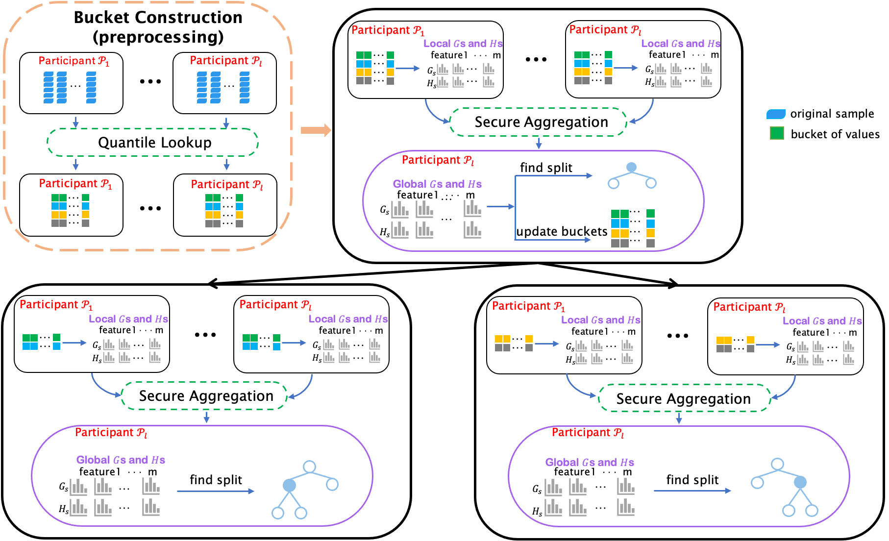
Figure 4: Horizontal FederBoost

5.2 Training

Similar to vertical FederBoost, bucket construction in horizontal FederBoost also only needs to be done once: participants can run training phase multiple times to fine-tune the model without further bucket construction as long as the data remains unchanged.

After finding all quantiles, each participant can locally put their sample IDs into the corresponding buckets; $\mathcal{P}_{l}$ can collect the buckets and aggregate them. Then, the setting becomes similar to vertical FederBoost. However, $\mathcal{P}_{l}$ does not hold all labels, hence it cannot train the decision trees as vertical FederBoost.

To this end, we take another approach, the pseudo-code of which is shown in Protocol 4. The key difference is that instead of sending the buckets of sample IDs to $\mathcal{P}_{l}$, each $\mathcal{P}_{i}$ locally computes $g$s and $h$s for each sample (line 9), computes $G$s and $H$s for each bucket (line 18) and all participants aggregates $G$s and $H$s for the corresponding buckets using secure aggregation (line 20). We remark that all $m\cdot q$ instances of secure aggregation can run in parallel. Another difference is that $\mathcal{P}_{l}$ needs to send the split information to all the other participants (line 24).

Naively, we can use the secure aggregation (cf. Appendix 2.3) protocol [18] by having $\mathcal{P}_{l}$ play the role of the parameter server. However, we simplify the protocol based on the assumption that the participants will not drop out in our setting. The pseudo-code is shown in Protocol 5. Notice that the gradients $G$s are floating-point numbers. To deal with this, we scale the floating-point numbers up to integers by multiplying the same constant to all values and drop the fractional parts. This idea is widely used in neural network training and inferences [31, 32]. $N$ must be large enough so that the absolute value of the final sum $G$ is smaller than $\left\lfloor N/2\right\rfloor$. We separately detail the security analysis of horizontal FederBoost from the perspective of $\mathcal{P}_{i}$ and $\mathcal{P}_{l}$ in Section 5.3. The whole process of horizontal FederBoost is visualized in Figure 4.

5.3 Security analysis

$\mathcal{P}_{i}$’s security. There are two places for potential information leakage:

• During quantile lookup, $\mathcal{P}_{i}$ inputs $n^{\prime}_{i}$ to secure aggregation (line 9 of Protocol 3).

• During tree construction, $\mathcal{P}_{i}$ inputs $G^{i}_{j,k}$ and $H^{i}_{j,k}$ to secure aggregation (line 20 of Protocol 4).

Both inputs are protected by secure aggregation. Although $\mathcal{P}_{l}$ can collude with $\tau-1$ passive participants, it still cannot learn anything beyond the sum of $l-\tau$ participants’ inputs.

$\mathcal{P}_{l}$’s security. There are again two places for potential information leakage:

• During quantile lookup, $\mathcal{P}_{l}$ sends $Q_{j}$ to other $\mathcal{P}$s (line 5 of Protocol 3).

• During tree construction, $\mathcal{P}_{l}$ sends $\mathit{split}_{j}$ to other $\mathcal{P}$s (line 24 of Protocol 4).

Notice that $Q_{j}$ is calculated based on $n^{\prime}$ and $\mathit{split}_{j}$ is calculated based on $G^{i}_{j}$ and $H^{i}_{j}$. Therefore, the information leakage of $\mathcal{P}_{l}$ will not be larger than $\mathcal{P}_{i}$ ($\mathcal{P}_{i}$’s security was proved above).

6 Implementation and Experiments

In this section, we evaluate FederBoost by conducting experiments on three public datasets:

• Credit 1: It is a credit scoring dataset used to predict the probability that somebody will experience financial distress in the next two years. It consists of a total of 150 000 samples and 10 features.

• Credit 2: It is another credit scoring dataset correlated to the task of predicting whether a user will make payment on time. It consists of a total of 30 000 samples and 23 features.

• SUSY: It is a dataset about high-energy physics, used to distinguish between a process where new super-symmetric particles are produced leading to a final state in which some particles are detectable, and others are invisible to the experimental apparatus. The original dataset consists of 3 000 000 samples and we choose 290 000 samples randomly from the dataset. Each sample has 18 features.

For each dataset, we divide it into two parts for training and testing respectively. The training part contains two-thirds of the samples and the testing part has the remaining one-third. We use the commonly used Area under the ROC curve (AUC) as the evaluation metric since the negative samples accounted for most of the samples in the Credit 1 dataset.

Our evaluation consists of two parts: utility and efficiency. Recall that, all participants jointly run the GBDT training algorithm in both vertical and horizontal FederBoost, hence varying the number of participants will not affect the utility of FederBoost. When evaluating utility, we only consider different number of buckets and different level of DP. We consider different number of participants when evaluating efficiency.

For “Credit 1” and “Credit 2”, we set the number of trees as $T=20$ and each tree has 3 layers; for “SUSY”, we set the number of trees as $T=60$ and each tree has 4 layers. All experiments were repeated 5 times and the averages are reported.

6.1 Utility

We first evaluate the utility of FederBoost with different number of buckets. Then, we fix the number of buckets with an optimal value and run vertical FederBoost with different level of DP (recall that DP is not needed for horizontal FederBoost).

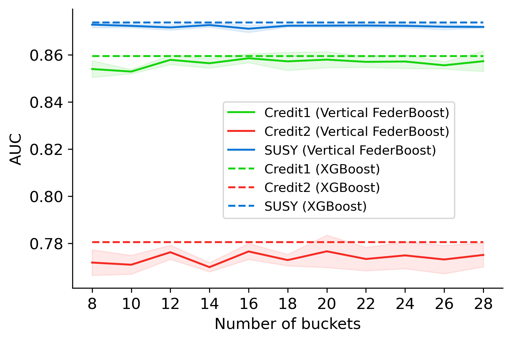
(a) Vertical FederBoost.

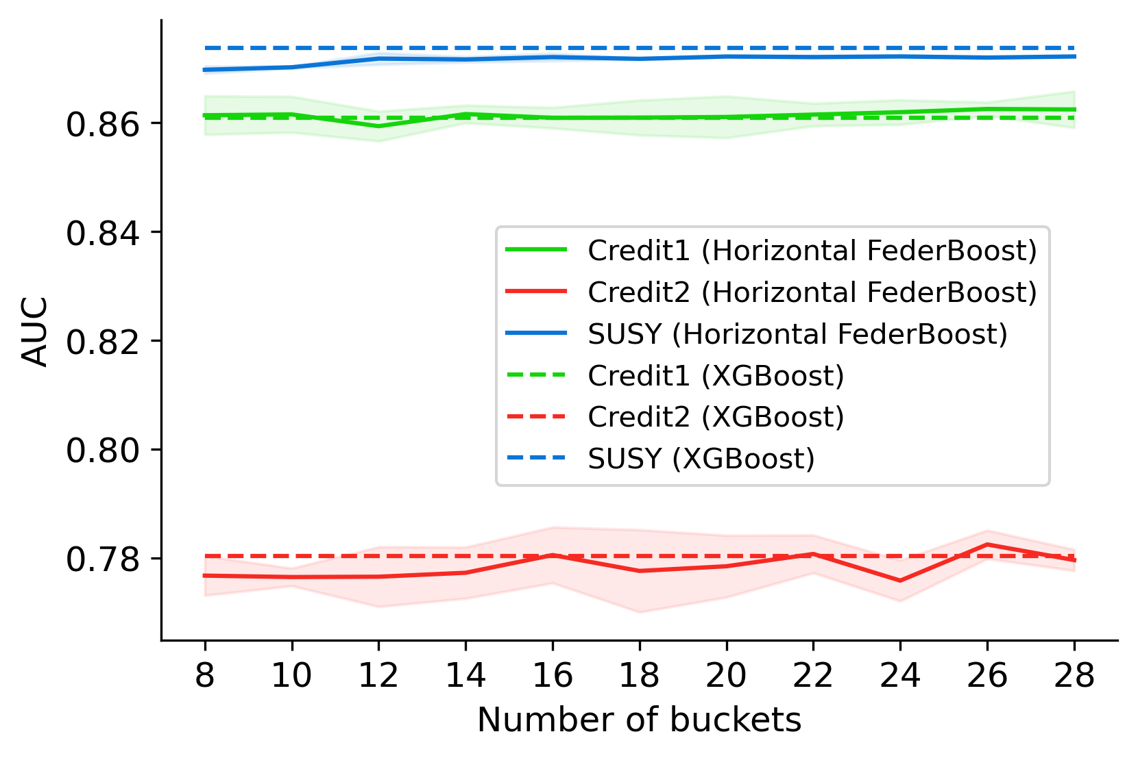
(b) Horizontal FederBoost.

Figure 5: Utility of FederBoost with different number of buckets (Left) and different level of DP (Right)

 

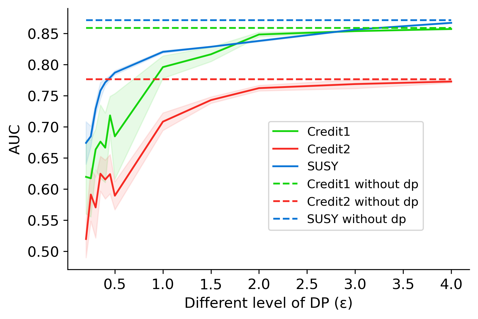
(c) Vertical FederBoost under DP.

We also run XGBoost centrally with the same datasets and use the results as baselines. As shown in Figure 5(b), FederBoost achieves almost the same accuracy with XGBoost. For “Credit 1”, the AUC achieved by XGBoost is 86.10% ; the best AUC achieved by vertical FederBoost is 85.85% with 16 buckets; and the best AUC achieved by horizontal FederBoost is 86.25% with 26 buckets. For “Credit 2”, the AUC achieved by XGBoost is 78.04% ; the best AUC achieved by vertical FederBoost is 77.65% with 16 buckets; and the AUC achieved by horizontal FederBoost is 78.25% with 24 buckets. For “SUSY”, the AUC achieved by XGBoost is 87.37%; the AUC achieved by vertical FederBoost is 87.26% with 14 buckets; and the AUC achieved by horizontal FederBoost is 87.22% with 24 buckets.

The performance of horizontal FederBoost is better than vertical FederBoost since we bucketize samples according to their quantile, which can better characterize the distribution of data. In contrast, samples are equally partitioned into different buckets in vertical FederBoost. Unfortunately, we cannot adopt the same strategy in vertical FederBoost since this will leak more information: in vertical FederBoost, each passive participant sends the sample IDs in each bucket to the active participant. In contrast, horizontal FederBoost only requires inputting the gradient of each bucket to secure aggregation. Meanwhile, the AUC for ”USPS” is more stable than ”Credit 1” and “Credit 2” since ”USPS” contains more samples, which can help train a more robust model.

Next, we set the number of buckets as 16 and run vertical FederBoost with different level of DP. Figure 5(c) shows the results. When $\epsilon$=4, the accuracy achieved by vertical FederBoost is very close to that without DP for all the three datasets. For “Credit 1”, vertical FederBoost achieves 85.70% accuracy when $\epsilon=4$ (it achieves 85.85% when no DP added). For “Credit 2”, vertical FederBoost achieves 77.27% accuracy when $\epsilon=4$ (it achieves 77.65% when no DP added). For “SUSY”, vertical FederBoost achieves 86.69% accuracy when $\epsilon=4$ (it achieves 87.10% when no DP added).

6.2 Efficiency

We fully implement FederBoost in C++ using GMP for cryptographic operations. We deploy our implementation on a machine that contains 40 2.20GHz CPUs, 251 GB memory; we spawn up to 32 processes, and each process runs as a single participant. For communication overhead, we consider both local area network (LAN) and wide area network (WAN). To simulate WAN, we limit the network bandwidth of each process to 20Mbit/s and add 100ms latency to each link connection.

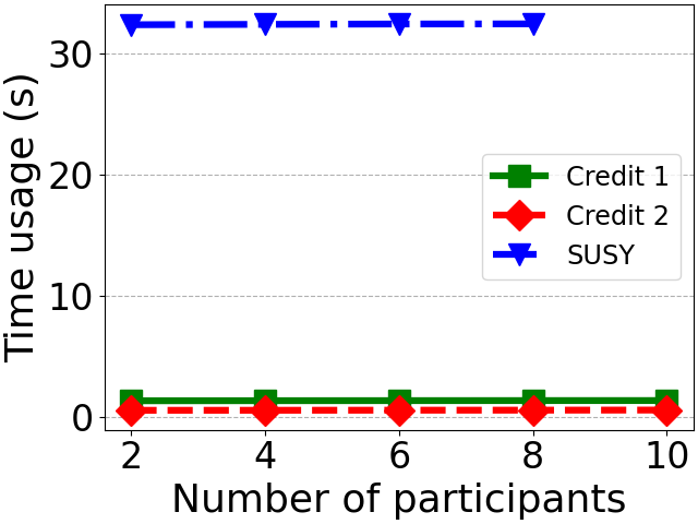
(a) Vertical FederBoost

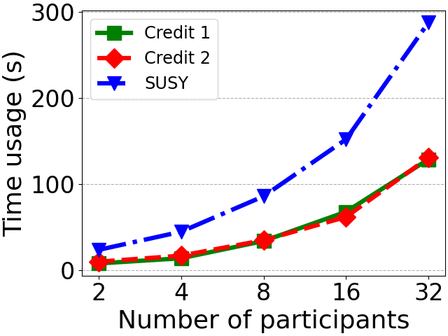
(b) Horizontal FederBoost

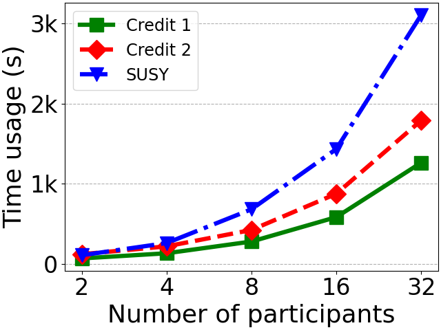
(d) Horizontal FederBoost

Figure 6: Training time of FederBoost with different number of participants w.r.t. LAN (Left) and WAN (Right)

 

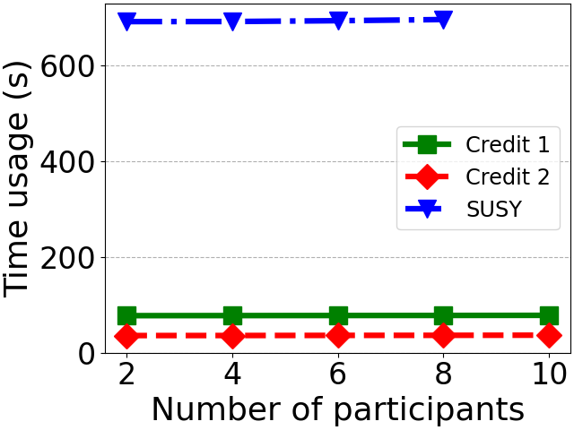
(c) Vertical FederBoost

Figure 6(a) shows the training time of vertical FederBoost in LAN with different number of participants. The results show that vertical FederBoost is very efficient: even for the challenging “SUSY” dataset, it only takes at most 33 seconds to train a GBDT model.

Figure 6(b) shows the training time of horizontal FederBoost in LAN. Both the bucket construction phase and the training phase require secure aggregation for each quantile lookup and each tree node split respectively. Recall that the efficiency of secure aggregation depends on the number of participants, hence the time usage of horizontal FederBoost increases linearly with the number of participants. For the “SUSY” dataset, it takes 23.75 seconds for 2 participants and 86 seconds for 8 participants. The results for “Credit1” and “Credit2” are similar: around 10 seconds for 2 participants and 130 seconds for 32 participants.

Figure 6(c) shows the training time of vertical FederBoost in WAN. In “SUSY”, it takes at most 691.77 seconds to train a GBDT model. Compared to LAN, the training time increases significantly, because passive participants need to transfer buckets of IDs to the active participant, which is expensive in WAN. Figure 6(d) shows the training time of horizontal FederBoost in WAN. It takes at most 3103.24 seconds to finish training.

Notice that the bucket construction phase only needs to be done once in either vertical FederBoost or horizontal FederBoost. It occupies more than half of the total time usage. If we remove bucket construction from the results, it will show a significant speedup.

We also compare FederBoost with Abspoel et al. [16] and Wu et al. [17], which are the state-of-the-art solutions for federated decision tree training. Abspoel et al. [16] is based on three party honest-majority replicated secret sharing; in particular, they use oblivious sorting to sort the samples for each feature. This scheme supports both vertically and horizontally partitioned data, but can only support three participants. They simulated each participant using a 2.5 GHz CPU. Moreover, their benchmarks were conducted in LAN with a dataset consisting of 8 192 samples and 11 features; they train 200 trees and each tree has 4 layers. We tailor our SUSY dataset to the same dimension and evaluate vertical and horizontal FederBoost in the same setting. Table II shows our time usage compared with the results reported in Table 1 of [16]. Vertical FederBoost achieves 83 099 times speedup and horizontal FederBoost achieves 4 668 times speedup.

TABLE II: FederBoost vs. Abspoel et al. [16]
(200 4-layer trees, 8192 samples, 11 features, 3 participants)

Method	Time usage
Vertical FederBoost	1.213 s
Horizontal FederBoost	21.59 s
Abspoel et al. [16]	$\sim$28 hours

Wu et al. [17] combine threshold partially homomorphic encryption (TPHE) with MPC. This scheme only supports vertically partitioned data. They simulated each participant using a 3.5 GHz CPU. Their benchmarks were conducted in LAN with a dataset consisting of 50 000 samples and 15 features; they train up to 32 trees and each tree has 4 layers. We also tailor our SUSY dataset to the same dimension and evaluate vertical FederBoost in the same setting. Table III shows our time usage compared with the results reported in Figure 4(f) of [17]. FederBoost achieves 1 111 times speedup.

TABLE III: FederBoost vs. Wu et al. [17]
(32 4-layer trees, 50 000 samples, 15 features, 3 participants)

Method	Time usage
Vertical FederBoost	32.4 s
Wu et al. [17]	$\sim$10 hours

7 Related Work

Horizontal federated learning. The terminology of FL was first proposed by Google in 2017. It allows multiple participants to jointly train a global model. It assumes the dataset is horizontally partitioned, and each participant transfers the locally trained model instead of the data. Quantization [3, 33] is a potential way to further reduce its communication overhead, which enables each client to send an efficient representation of the model without affecting much of the utility. FL also brings new security and privacy risks. A backdoor can be injected to the global model to make it achieve high accuracy on both its main task and the backdoor subtask. A naive approach is to have the attacker train the local model with poisoned local data, which is called data poisoning attacks. Even worse, the attacker can directly manipulate its gradients to make the backdoor more difficult to be detected, which is called model poisoning attacks [34]. In privacy perspective, Melis et al. [35] show that an attacker can infer properties of others’ training data even if such properties are independent of the classes of the global model. We leave it as future work to prevent such poisoning attacks and information leakage in FederBoost.

Vertical federated learning. Hardy et al. [10] came up with a protocol that enables two participants to run logistic regression over vertically partitioned data. They approximate logistic regression using Taylor series to make it friendly to homomorphic encryption. The two participants encrypt their partial gradients using an encryption key that belongs to an independent third party, and homomorphically combine the ciphertexts to get the encrypted gradients. The third party decrypts the ciphertext and returns the gradients to both participants, who can then update their model parameters. Even though this protocol has been deployed in an industrial-level federated learning framework named FATE [11], it provides a low privacy level: a participant can easily get the other’s partial gradients from the returned value; then it is equal to directly exchanging the partial gradients between these two participants (no need to use either homomorphic encryption or third party).

SecureML [31] targets the setting where data owners distribute their private data to two non-colluding servers to train models using secure two-party computation (2PC). We can slightly change the setting to make it work as a vertical FL scheme. More specifically, we have each server play the role of a data owner as well; they hold different set of features and one of them holds the labels. However, the protocol is too slow to be used in practice: their experimental results show that it takes at least 3.4 days to train a two-layer neural network with a dataset that consists of 60 000 samples and 784 features.

Besides the cryptographic approaches, there are also some work try to build vertical FL from a machine learning point of view. In another work named FDML [36], each participant trains a separate model using its own feature space and shares the prediction result to others (through a central server). A central server aggregates the prediction results; all participants update their models based on the aggregated result and move to the next round. FDML involves no cryptographic operation, but requires all participants to know the labels to train models locally, which is unrealistic in real-world. Usually, only a single participant holds the labels and other participants only have the features.

Federated Decision Tree Learning. In addition to the solutions proposed by Abspoel et al. [16] and Wu et al. [17] (cf. Section 6.2), there are some other work that solve the problem of federated decision tree training. Even though not specifically mentioned, the first federated decision tree learning algorithm was proposed by Lindell and Pinkas in 2000 [15]. They came up with a protocol allowing two participants to privately compute the ID3 algorithm over horizontally partitioned data. Recently, Cheng et al. [14] propose SecureBoost, a federated GBDT framework for vertically partitioned data. In SecureBoost, $\mathcal{P}_{l}$ calculates $g_{i}$s and $h_{i}$s for all samples, encrypts them using additively homomorphic encryption, and sends the ciphertexts $\left\langle g_{i}\right\rangle$s and $\left\langle h_{i}\right\rangle$s to all other participants. This protocol is expensive since it requires cryptoraphic computation and communication for each possible split. As a comparison, our vertical FederBoost does not require any cryptographic operation. Chen et al. [37] incorporates several engineering optimizations into SecureBoost. Experiments on the Credit2 dataset show that it requires at least 30 seconds to train a single tree, while we only require 2 seconds to train 20 trees.

Another recent work [38] for federated GBDT was achieved using trusted execution environments (TEEs) [39, 40]. It introduces a central server that is equipped with a TEE. All participants send their data, no matter vertically or horizontally partitioned, to the TEE via secure channels. However, TEEs are known to be vulnerable to hardware based side-channel attacks [41]. Alternatively, Li et al. [42] apply locality sensitive hashing (LSH) to federated GBDT. However, their solution only supports horizontally partitioned data, and the security of LSH is difficult to quantify. Zhu et al. [43] considers a setting where the data is vertically partitioned but the labels are distributed among multiple clients whereas we assume the labels are stored only on one client. Furthermore, they only protect the privacy of labels, whereas we protect both data and labels.

8 Conclusion

In response to the growing demand for a federated GBDT framework, we propose FederBoost that supports running GBDT privately over both vertically and horizontally partitioned data. Vertical FederBoost does not require any cryptographic operation and horizontal FederBoost only requires lightweight secure aggregation. Our experimental results show that both vertical and horizontal FederBoost achieves the same level of accuracy with centralized training; and they are 4-5 orders of magnitude faster than the state-of-the-art solution for federated decision tree training.

In future work, we will further improve the performance of FederBoost. For example, we could optimize the communication among participants using some structured networks [44]. We will explore poisoning attacks targeting FederBoost and seek for solutions. We will attempt to deploy FederBoost in real industrial scenarios and check its performance on more realistic data.

References

- [1] B. McMahan, E. Moore, D. Ramage, S. Hampson, and B. A. y Arcas, “Communication-efficient learning of deep networks from decentralized data,” in Proceedings of the 20th International Conference on Artificial Intelligence and Statistics, A. Singh and J. Zhu, Eds., vol. 54. Fort Lauderdale, FL, USA: PMLR, 20–22 Apr 2017, pp. 1273–1282. [Online]. Available: http://proceedings.mlr.press/v54/mcmahan17a.html
- [2] S. U. Stich, “Local sgd converges fast and communicates little,” 2018.
- [3] J. Konečnỳ, H. B. McMahan, F. X. Yu, P. Richtárik, A. T. Suresh, and D. Bacon, “Federated learning: Strategies for improving communication efficiency,” arXiv preprint arXiv:1610.05492, 2016.
- [4] M. Assran, N. Loizou, N. Ballas, and M. Rabbat, “Stochastic gradient push for distributed deep learning,” CoRR, vol. abs/1811.10792, 2018. [Online]. Available: http://arxiv.org/abs/1811.10792
- [5] C. Xie, S. Koyejo, and I. Gupta, “Asynchronous federated optimization,” CoRR, vol. abs/1903.03934, 2019. [Online]. Available: http://arxiv.org/abs/1903.03934
- [6] T. Chen, G. B. Giannakis, T. Sun, and W. Yin, “Lag: Lazily aggregated gradient for communication-efficient distributed learning,” 2018.
- [7] M. Mohri, G. Sivek, and A. T. Suresh, “Agnostic federated learning,” CoRR, vol. abs/1902.00146, 2019. [Online]. Available: http://arxiv.org/abs/1902.00146
- [8] L. Lyu, H. Yu, X. Ma, L. Sun, J. Zhao, Q. Yang, and P. S. Yu, “Privacy and robustness in federated learning: Attacks and defenses,” arXiv preprint arXiv:2012.06337, 2020.
- [9] Q. Yang, Y. Liu, T. Chen, and Y. Tong, “Federated machine learning: concept and applications,” ACM Transactions on Intelligent Systems and Technology (TIST), vol. 10, no. 2, p. 12, 2019.
- [10] S. Hardy, W. Henecka, H. Ivey-Law, R. Nock, G. Patrini, G. Smith, and B. Thorne, “Private federated learning on vertically partitioned data via entity resolution and additively homomorphic encryption,” ArXiv, vol. abs/1711.10677, 2017.
- [11] FATE, “An industrial grade federated learning framework,” 2019, https://fate.fedai.org/.
- [12] F. Fu, Y. Shao, L. Yu, J. Jiang, H. Xue, Y. Tao, and B. Cui, “Vfboost: Very fast vertical federated gradient boosting for cross-enterprise learning,” in SIGMOD ’21: International Conference on Management of Data, Virtual Event, China, June 20-25, 2021, G. Li, Z. Li, S. Idreos, and D. Srivastava, Eds. ACM, 2021, pp. 563–576. [Online]. Available: https://doi.org/10.1145/3448016.3457241
- [13] T. Chen and C. Guestrin, “Xgboost: A scalable tree boosting system,” in Proceedings of the 22nd ACM SIGKDD International Conference on Knowledge Discovery and Data Mining, ser. KDD ’16. New York, NY, USA: Association for Computing Machinery, 2016, p. 785–794. [Online]. Available: https://doi.org/10.1145/2939672.2939785
- [14] K. Cheng, T. Fan, Y. Jin, Y. Liu, T. Chen, and Q. Yang, “Secureboost: A lossless federated learning framework,” CoRR, vol. abs/1901.08755, 2019. [Online]. Available: http://arxiv.org/abs/1901.08755
- [15] Y. Lindell and B. Pinkas, “Privacy preserving data mining,” in Advances in Cryptology — CRYPTO 2000, M. Bellare, Ed. Berlin, Heidelberg: Springer Berlin Heidelberg, 2000, pp. 36–54.
- [16] M. Abspoel, D. Escudero, and N. Volgushev, “Secure training of decision trees with continuous attributes,” IACR Cryptol. ePrint Arch., vol. 2020, p. 1130, 2020. [Online]. Available: https://eprint.iacr.org/2020/1130
- [17] Y. Wu, S. Cai, X. Xiao, G. Chen, and B. C. Ooi, “Privacy preserving vertical federated learning for tree-based models,” Proc. VLDB Endow., vol. 13, no. 11, pp. 2090–2103, 2020. [Online]. Available: http://www.vldb.org/pvldb/vol13/p2090-wu.pdf
- [18] K. Bonawitz, V. Ivanov, B. Kreuter, A. Marcedone, H. B. McMahan, S. Patel, D. Ramage, A. Segal, and K. Seth, “Practical secure aggregation for privacy-preserving machine learning,” in Proceedings of the 2017 ACM SIGSAC Conference on Computer and Communications Security. ACM, 2017, pp. 1175–1191.
- [19] J. Jiang, B. Cui, C. Zhang, and F. Fu, “Dimboost: Boosting gradient boosting decision tree to higher dimensions,” in Proceedings of the 2018 International Conference on Management of Data, ser. SIGMOD ’18. New York, NY, USA: Association for Computing Machinery, 2018, p. 1363–1376. [Online]. Available: https://doi.org/10.1145/3183713.3196892
- [20] F. Fu, J. Jiang, Y. Shao, and B. Cui, “An experimental evaluation of large scale gbdt systems,” Proc. VLDB Endow., vol. 12, no. 11, p. 1357–1370, Jul. 2019. [Online]. Available: https://doi.org/10.14778/3342263.3342273
- [21] C. Dwork, “Differential privacy: a survey of results,” in Theory and Applications of Models of Computation—TAMC, ser. Lecture Notes in Computer Science, vol. 4978. Springer Verlag, April 2008, pp. 1–19. [Online]. Available: https://www.microsoft.com/en-us/research/publication/differential-privacy-a-survey-of-results/
- [22] M. Abadi, A. Chu, I. Goodfellow, H. B. McMahan, I. Mironov, K. Talwar, and L. Zhang, “Deep learning with differential privacy,” in Proceedings of the 2016 ACM SIGSAC Conference on Computer and Communications Security, ser. CCS ’16. New York, NY, USA: Association for Computing Machinery, 2016, p. 308–318. [Online]. Available: https://doi.org/10.1145/2976749.2978318
- [23] Q. Li, Z. Wu, Z. Wen, and B. He, “Privacy-preserving gradient boosting decision trees,” Proceedings of the AAAI Conference on Artificial Intelligence, vol. 34, no. 01, pp. 784–791, Apr. 2020. [Online]. Available: https://ojs.aaai.org/index.php/AAAI/article/view/5422
- [24] G. Ke, Q. Meng, T. Finley, T. Wang, W. Chen, W. Ma, Q. Ye, and T.-Y. Liu, “Lightgbm: A highly efficient gradient boosting decision tree,” in Advances in Neural Information Processing Systems 30, I. Guyon, U. V. Luxburg, S. Bengio, H. Wallach, R. Fergus, S. Vishwanathan, and R. Garnett, Eds. Curran Associates, Inc., 2017, pp. 3146–3154. [Online]. Available: http://papers.nips.cc/paper/6907-lightgbm-a-highly-efficient-gradient-boosting-decision-tree.pdf
- [25] V. Kolesnikov, N. Matania, B. Pinkas, M. Rosulek, and N. Trieu, “Practical multi-party private set intersection from symmetric-key techniques,” in Proceedings of the 2017 ACM SIGSAC Conference on Computer and Communications Security, ser. CCS ’17. New York, NY, USA: Association for Computing Machinery, 2017, p. 1257–1272. [Online]. Available: https://doi.org/10.1145/3133956.3134065
- [26] S. Wang, L. Huang, P. Wang, H. Deng, H. Xu, and W. Yang, “Private weighted histogram aggregation in crowdsourcing,” in Wireless Algorithms, Systems, and Applications, Q. Yang, W. Yu, and Y. Challal, Eds. Cham: Springer International Publishing, 2016, pp. 250–261.
- [27] Tin Kam Ho, “Random decision forests,” in Proceedings of 3rd International Conference on Document Analysis and Recognition, vol. 1, 1995, pp. 278–282 vol.1.
- [28] L. Breiman, “Bagging predictors,” Machine Learning, vol. 24, no. 2, pp. 123–140, 1996.
- [29] E. Gan, J. Ding, K. S. Tai, V. Sharan, and P. Bailis, “Moment-based quantile sketches for efficient high cardinality aggregation queries,” Proc. VLDB Endow., vol. 11, no. 11, p. 1647–1660, Jul. 2018. [Online]. Available: https://doi.org/10.14778/3236187.3236212
- [30] Z. Karnin, K. Lang, and E. Liberty, “Optimal quantile approximation in streams,” in 2016 IEEE 57th Annual Symposium on Foundations of Computer Science (FOCS), 2016, pp. 71–78.
- [31] P. Mohassel and Y. Zhang, “Secureml: A system for scalable privacy-preserving machine learning,” in 2017 IEEE Symposium on Security and Privacy (SP), May 2017, pp. 19–38.
- [32] J. Liu, M. Juuti, Y. Lu, and N. Asokan, “Oblivious neural network predictions via minionn transformations,” in Proceedings of the 2017 ACM SIGSAC Conference on Computer and Communications Security, ser. CCS ’17. New York, NY, USA: Association for Computing Machinery, 2017, p. 619–631. [Online]. Available: https://doi.org/10.1145/3133956.3134056
- [33] Y. Lin, S. Han, H. Mao, Y. Wang, and W. J. Dally, “Deep gradient compression: Reducing the communication bandwidth for distributed training,” arXiv preprint arXiv:1712.01887, 2017.
- [34] E. Bagdasaryan, A. Veit, Y. Hua, D. Estrin, and V. Shmatikov, “How to backdoor federated learning,” CoRR, vol. abs/1807.00459, 2018. [Online]. Available: http://arxiv.org/abs/1807.00459
- [35] L. Melis, C. Song, E. De Cristofaro, and V. Shmatikov, “Exploiting unintended feature leakage in collaborative learning,” in 2019 IEEE Symposium on Security and Privacy (SP), 2019, pp. 691–706.
- [36] Y. Hu, D. Niu, J. Yang, and S. Zhou, “FDML: A collaborative machine learning framework for distributed features,” in Proceedings of the 25th ACM SIGKDD International Conference on Knowledge Discovery & Data Mining, ser. KDD ’19. New York, NY, USA: ACM, 2019, pp. 2232–2240. [Online]. Available: http://doi.acm.org/10.1145/3292500.3330765
- [37] W. Chen, G. Ma, T. Fan, Y. Kang, Q. Xu, and Q. Yang, “Secureboost+ : A high performance gradient boosting tree framework for large scale vertical federated learning,” CoRR, vol. abs/2110.10927, 2021. [Online]. Available: https://arxiv.org/abs/2110.10927
- [38] Andrew Law, Chester Leung, Rishabh Poddar, Raluca Ada Popa, Chenyu Shi, Octavian Sima, Chaofan Yu, Xingmeng Zhang, and Wenting Zheng, “Secure collaborative training and inference for xgboost,” in Workshop on Privacy-Preserving Machine Learning in Practice (PPMLP’ 20), 2020.
- [39] “AMD Secure Processor,” http://www.amd.com/en-us/innovations/software-technologies/security.
- [40] Intel, “Software Guard Extensions (Intel SGX) Programming Reference,” 2013, https://software.intel.com/sites/default/files/managed/48/88/329298-002.pdf.
- [41] J. Van Bulck, M. Minkin, O. Weisse, D. Genkin, B. Kasikci, F. Piessens, M. Silberstein, T. F. Wenisch, Y. Yarom, and R. Strackx, “Foreshadow: Extracting the keys to the intel sgx kingdom with transient out-of-order execution,” in Proceedings of the 27th USENIX Conference on Security Symposium, ser. SEC’18. Berkeley, CA, USA: USENIX Association, 2018, pp. 991–1008. [Online]. Available: http://dl.acm.org/citation.cfm?id=3277203.3277277
- [42] Q. Li, Z. Wen, and B. He, “Practical federated gradient boosting decision trees,” CoRR, vol. abs/1911.04206, 2019. [Online]. Available: http://arxiv.org/abs/1911.04206
- [43] H. Zhu, R. Wang, Y. Jin, and K. Liang, “PIVODL: privacy-preserving vertical federated learning over distributed labels,” CoRR, vol. abs/2108.11444, 2021. [Online]. Available: https://arxiv.org/abs/2108.11444
- [44] J. Bell, K. Bonawitz, A. Gascón, T. Lepoint, and M. Raykova, “Secure single-server aggregation with (poly)logarithmic overhead,” IACR Cryptol. ePrint Arch., vol. 2020, p. 704, 2020. [Online]. Available: https://eprint.iacr.org/2020/704