Possibility of primordial black holes as the source of gravitational wave events in the advanced LIGO detector

Abstract

The analysis of gravitational Wave (GW) data from advanced LIGO provides the mass of each companion of binary black holes as the source of GWs. The mass of events corresponding to the binary black holes from GW is above $20$ M_⊙ which is much larger than the mass of astrophysical black holes detected by x-ray observations. In this work, we examine primordial black holes (PBHs) as the source of LIGO events. Assuming that $100\%$ of the dark matter is made of PBHs, we estimate the rate at which these objects make binaries, merge, and produce GWs as a function of redshift. The gravitational lensing of GWs by PBHs can also enhance the amplitude of the strain. We simulate GWs sourced by binary PBHs, with the detection threshold of $S/N>10$ for both Livingston and Hanford detectors. For the log-normal mass function of PBHs, we generate the expected distribution of events, compare our results with the observed events, and find the best value of the mass function parameters (i.e., $M_{c}=25M_{\odot}$ and $\sigma=0.6$) in the log-normal mass function. Comparing the expected number of events with the number of observed ones rules out the present-Universe binary formation PBH scenario as the candidate for the source of GW events detected by LIGO.

The recent discovery of gravitational waves (GWs) by advanced LIGO, sourced from binary black hole mergers, opened a new window in astronomy. The analysis of strain signals with theoretical templates of the GW can determine the mass of binary black holes (BBHs) Abbott et al. (2019a). Since the mass of black holes from GWs are larger than the astrophysical black holes discovered yet by x-ray observation Casares et al. (2017), one of the possibilities could be that the source of observed GWs is due to primordial black holes (PBHs). Ten GW candidates are detected as a result of the first and second runs of advanced LIGO (i.e., O1 and O2) Abbott et al. (2019a) and VIRGO Acernese et al. (2015) in $48.6$ day and $117$ day runs, respectively Abbott et al. (2016a, 2017). During the third observing run $O_{3}$ (i.e., April $2019$-March $2020$)oii with the improved sensitivity of detectors Acernese et al. (2019); Tse et al. (2019), ten candidate GW events have been identified oi ; however, four events have been confirmed Abbott et al. (2020a, b, c, d).

As pointed in Refs. Carr et al. (2017, 2020), and references therein, PBHs cannot make all the dark matter regarding the monochromatic mass function. Several scenarios to describe the formation of PBHs based on the collapse of large density perturbation in the radiation-dominated era propose an extended mass function for PBHs Kühnel and Freese (2017); Niemeyer and Jedamzik (1998). That would make possible that PBHs with an extended mass function make all dark matter of the UniverseCarr et al. (2017, 2020); Green (2016).

In this work, we adapt the log-normal mass function for the PBHs Carr et al. (2017); Kannike et al. (2017); Dolgov and Silk (1993) as

$$\psi(M)=\frac{f_{PBH}}{\sqrt{2\pi}\sigma M}\exp\left(-\frac{log^{2}({M}/{M_{c}})}{2\sigma^{2}}\right),$$ (1)

where $M_{c}$ is characteristic mass, $\sigma$ is the width of mass function, and $f_{PBH}$ is the fraction of dark matter made of PBHs.

While PBHs in the early universe were produced individually, we can argue that a very small fraction of them can make binary systems in a cosmological timescale. When two individual PBHs pass close to each other, as a result of gravitational interaction, they can radiate GWs. For efficient interaction, PBHs can make binary systems due to the dissipation process of GW emission surpassing their initial kinetic energy Bird et al. (2016). The rate of binary formation per halo is given by Bird et al. (2016)

$$R(M)=\int_{0}^{R_{\rm vir}}2\pi r^{2}\Big{(}\frac{\rho_{\rm nfw}(r)}{M_{\rm pbh}}\Big{)}^{2}\langle\sigma_{GW}v_{\rm pbh}\rangle dr,$$ (2)

where $\sigma=\pi(\frac{85\pi}{3})^{2/7}R_{\rm s}^{2}(\frac{v_{\rm pbh}}{c})^{18/7}$ is the cross section for binary formation Quinlan and Shapiro (1989); Mouri and Taniguchi (2002). $\rho_{\rm nfw}=\rho_{s}[(r/R_{s})(1+r/R_{s})^{2}]^{-1}$ is the Navarro-Frenk-White (NFW) density profile with characteristic radius and density $R_{s}$ and $\rho_{s}$, respectively. $R_{\rm vir}$ is the virial radius of the galactic halo at which the density of NFW profile reaches 200 times the mean cosmic density. $v_{\rm pbh}$ is the dispersion velocity of PBHs, and $M_{\rm pbh}$ is the mass of the PBH.

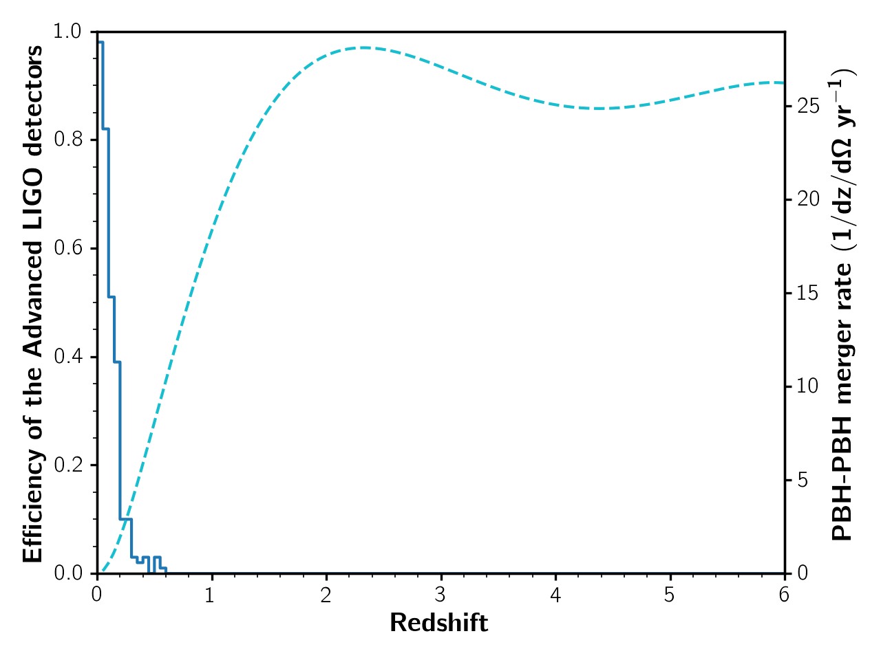
Figure 1: The dashed line represents the total PBH merger rate per steradian per redshift per year from Eq. (4). Here, we assume that 100% of dark matter is made of PBHs. The solid-line histogram shows the redshift dependence of the efficiency of advanced LIGO with $SNR>10$ detection threshold.

After the binary formation stage, the binary system can further emit GWs, lose orbital energy, and finally inspiral to merge. This merging happens on a timescale which is much smaller than the Hubble time at $z=0$, and, hence, at the current time, we can safely assume that once a binary is formed, it will certainly also merge to produce GWs Bird et al. (2016). In order to estimate how far back we can go in time to have the first merging, we compare the merging timescale O’Leary et al. (2009) with the age of the Universe [i.e., ${4\pi GM_{tot}}/{v_{pbh}^{3}}\sim 1/H(z)$]. Numerical estimation from this equation results in $z\approx 6$.

In what follows, we estimate the number of binary PBHs that can be formed from single PBHs. We follow the work of Bird et al. Bird et al. (2016), where the calculation is done for the local Universe. The total merger rate per unit volume is as follows:

$$\Gamma=\int\frac{dn}{dM}R(M)dM,$$ (3)

where $dn/dM$ is the halo mass function that we adopt the Press-Schechter formalism Press and Schechter (1974) and $R(M)$ from Eq. (2) is the rate of mergers in a given halo of mass $M$.

Considering that halos are formed at the higher redshifts Ludlow et al. (2016), we take into account the redshift dependence in Eq. (3) and write the rate of events in comoving volume as

$$\frac{dN(z)}{dzd\Omega}=c\frac{\chi^{2}(z)}{H(z)}\int_{0}^{M_{vir}(z)}\frac{dn(z)}{dM}R(M,z)dM,$$ (4)

where $c$ is the speed of light, $\chi(z)$ is the comoving distance, $H(z)$ is the Hubble expansion rate, and $dn(z)/dM$ is the halo mass function of halos at the redshift $z$. It should be noted that the upper limit of the integral decreases with increasing the redshift where at the higher redshifts the larger-mass halos have not been virialized yet Loeb et al. (2008).

From Eq. (4), we plot $dN(z)/{dzd\Omega}$ in Fig. 1 (dashed line) as the merging rate per redshift per steradian per year, assuming that $100\%$ of dark matter is made of PHBs. It is noteworthy that the peak at $z\approx 2$ results from the peaking comoving volume at this redshift. Integrating the curve in Fig. 1 over the redshift, the result is about $1724$ events per year for $z<6$. However, as we will determine the detection efficiency of LIGO, only the close-by events can be detected. GW signals for distant sources can also be magnified by gravitational lensing. Assuming the whole dark matter is made of PBHs, they can also play the role of lensing.

In what follows, we simulate the GWs from PBHs binary merging in the Universe and measure the detectability of events by LIGO detector. For simulating an ensemble of GW sources and lenses, we assume (a) a mass function for PBHs is log normal Carr et al. (2017) and (b) the redshift distribution of the PBHs follows the comoving volume. Then we calculate the antenna pattern function for Hanford and Livingston and include the background noise to determine GW strain in the detector frame Abbott et al. (2019a); pyc .

In the next step, we calculate the microlensing optical depth as a function of redshift to calculate the number of GWs being lensed. The optical depth as the probability of lensing for a homogeneous distribution of PBHs is give by Zackrisson and Riehm (2007)

$$\tau=\frac{3H_{0}\Omega_{\rm PBH}}{2D_{\rm s}}\int_{0}^{z_{\rm s}}\frac{(1+z)^{2}D_{\rm ls}D_{\rm l}\rm dz}{c\sqrt{\Omega_{\rm M}(1+z)^{3}+\Omega_{\rm\Lambda}}},$$ (5)

where $H_{0}$ is the current value of the Hubble parameter, $\Omega_{\rm M}$ is the dark matter density parameter, and $\Omega_{\rm\Lambda}$ is the dark energy density parameter. $D_{\rm s}$, $D_{\rm ls}$, and $D_{\rm l}$ are the comoving observer-source distance, lens-source distance, and lens distance, respectively. Here, we assume PBHs composed the whole dark matter (i.e., $\Omega_{\rm M}=\Omega_{\rm PBH}$). Figure 2 (solid curve) shows the optical depth as a function of redshift. The multiplication of the optical depth, $\tau(z)$ by the event rate $N(z)$ would result in the rate of the microlensed-GW event. This rate is shown in Fig. 2 (dashed curve).

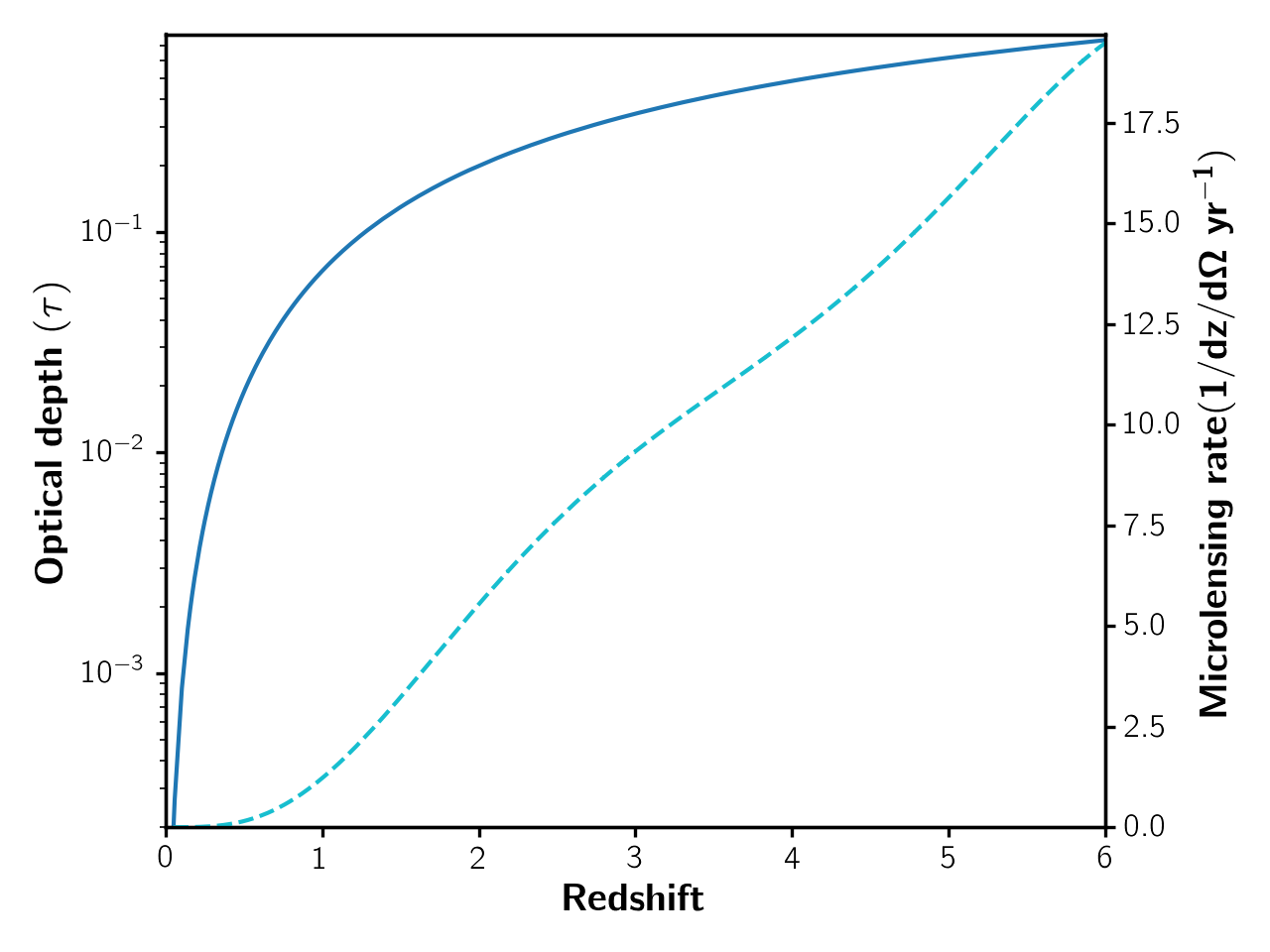
Figure 2: This plot assumes that the whole of dark matter is composed of PBHs(light blue). The multiplication of the optical depth $\tau(z)$ (dark blue curve) and the event rate, $N(z)$ as a function of the redshift. This curve represents the rate of microlensed GWs, sourced by PBHs.

In the gravitational lensing of gravitational waves, since the mass of the binary merging system is on the order of the lens, then the wavelength of GW $\lambda$ is on the order of the Schwarzchild radius of the lens, $R_{sch}$. In this case, we need to deal with the problem with the wave optics approach. The propagation of gravitational wave with a perturbation due to a lens behaves similar to the electromagnetic equation (i.e. $\square h^{\mu\nu}=0$) De Paolis et al. (2001); Takahashi and Nakamura (2003), where the metric is $g_{\mu\nu}=\eta_{\mu\nu}+h_{\mu\nu}$. The GWs can be magnified similar to the electromagnetic radiation during the microlensing; however, since the timescale of GW is very short, we can take a static configuration for the relative position of the source, lens and the observer.

From the generic solution of the wave equation, we can calculate the magnification factor for the strain of the GW during the lensing as Schneider et al. (1992)

$$\mu_{GW}(\beta;k)=\sqrt{\pi f}J_{0}(f\beta),$$ (6)

where $f=2kR_{\rm sch}$, $k$ is the wave number, $\beta$ is the impact parameter of the source on the lens plane normalized to the Einstein angle, and $J_{0}$ is the Bessel function of the first kind. We note that the magnification for light is the square of relation (6) as for the electromagnetic waves; we measure the intensity of light (i.e., $I\propto E^{2}$) while for the GW we measure the strain (i.e., $h_{\mu\nu}$). In the limit of $k\rightarrow\infty$, we can recover the geometric optics relation for the magnification. In our simulation, we limit the minimum impact parameter to be in the range of $0<\beta<1$.

In what follows, we consider log-normal mass functions for PBHs with different parameters of $M_{c}$ and $\sigma$ of Eq. (1). We perform a Monte Carlo simulation and generate binary PBHs over the redshift range of $(0-6)$. We also take into account the microlensing of the GWs with the magnification given by Eq. (6).

After generating GW events in our simulation, we add the corresponding noise to the data and use the specification of LIGO for calculating the detection efficiency of the LIGO detector. For analyzing simulated data, we use PyCBC inference Biwer et al. (2019) package with dynamic nested sampling Markov chain Monte Carlo algorithm, dynesty Speagle (2020). It is based on sampling the likelihood function for a hypothesis that gives a measure of the existence of a signal in the data. The sampler performs the full Bayesian parameter estimation for each injection. Then we can obtain the maximum SNR recovered from injection. We assume a threshold of $S/N>10$ for criteria of significant detection. For each injection, we used the inbuilt injection creation of the PyCBC package using the IMRPhenomPv2 waveform. We choose two detector networks (Hanford and Livingston) for this analysis. We run the pipeline for $16304\times 4\times 6$ [accounting for $M_{c}=20,25,30$, and $35M_{\odot}$ and $\sigma=0.1,0.2,0.3,0.4,0.5$, and $0.6$ of the model (1)] injections using detector sensitivity during the O2 run. It is known that LIGO noise varies over long periods of time Abbott et al. (2016b); in order to model the detector sensitivity (accounting for non-Gaussian and/or nonstationary background noise), we made $32^{\rm{Hanford}}\times 32^{\rm{Livingston}}=1024$ number of power spectral densities (PSD) of 4096 s random data and perform the PyCBC pipeline to analyse the injections for these random times. We used a fake Gaussian noise (via the fake-strain option) that is colored by a given PSD.

These injections are created with zero spin BBH components. The orientation (inclination and polarization angles ) and location (right ascension and declination) of the GW sources are distributed uniformly in the polarization sphere and in the sky, respectively Abbott et al. (2019a); Haris et al. (2018).

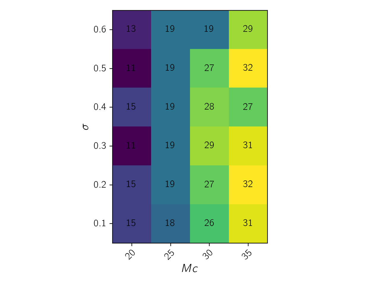
Figure 3: The number of detected events from the simulated events for source located at $z<1$, for various log-normal parameters of $\sigma$ and $M_{c}$ PBH mass function, assuming $f=1$.

In the following, we calculate the redshift-dependent detection efficiency function of advanced LIGO observatory as

$$\epsilon(z)=\frac{\Delta N_{detected}(z,z+\Delta z)}{\Delta N_{theory}(z,z+\Delta z)},$$ (7)

where $\Delta N_{detected}$ is the number of events with $SNR>10$ between $(z,z+\Delta z)$ and $\Delta N_{theory}$ is the number of theoretical events we generate between $(z,z+\Delta z)$. In Fig. 1, the histogram with a solid line represents the efficiency function of LIGO in terms of redshift. This function declines to zero at the redshift $z\simeq 0.6$. Multiplying the efficiency function by the normalized distribution of events based on the theoretical assumptions [i.e., $\Delta N_{expected}=\Delta N_{theory}\times\epsilon(z)$] results in the expected number of events.

In order to find the best parameters for the mass function of PBHs, we compare the mass distribution of observed GW sources with that of our simulated events Abbott et al. (2019a). Here, we use the mean and the width of the detected distribution of mass of events (derived from the analysis of the binary black hole) and compare them with the simulation. The log-normal mass function with a characteristic mass of $M_{c}=25M_{\odot}$ and $\sigma=0.6$ in Eq. (1) shown in Fig. (3) has the best compatibility between the theory and the observation.

Now, we compare the number of observed events with that of our expectations from the theory. Integrating $\Delta N_{expected}/dz$ over $z$, we calculate the overall expected number of events, where, according to the efficiency function, we are able to detect events up to a distance of $z\sim 0.6$. We note that in our simulation $38\%$ of GW events with high redshifts have been microlensed; however, for the lower redshifts (i.e., $z<1$), the number of microlensed events is negligible. The comparison of the observed GW events ( seven events from 117 days observation by O2) with the expected number of events assuming $100\%$ of dark matter is made of PBHs (0.5 event for 117 days) reveals that $N_{observed}\gg N_{expected}$, which means that $f>1$. In order to explain this result within the context of the scenario that has been used in this work, we propose the following two explanations. (i) The first possibility is that astrophysical black holes might be responsible for GW events instead of binary PBHs. The problem with this solution is that astrophysical black holes above $\sim$$20$ solar masses have not been discovered yet from direct x-ray observation. However, there are astrophysical scenarios for the formation of heavy black holes Belczynski et al. (2010); Spera et al. (2015). (ii) In this paper, we followed the formalism of PBH binary formation in the present Universe Bird et al. (2016). There is other scenario that suggests the formation of a PBH binary in the early Universe Sasaki et al. (2018). LIGO constraints the primordial black holes with a mass between $0.2$ M_⊙ $and$ $1.0$ M_⊙ using early-Universe PBH binary formation Abbott et al. (2018, 2019b). If we assume binary PBHs formation in early Universe, the number of binary black hole systems would increase and may explain the observed GW events.

References

- Abbott et al. (2019a) B. Abbott et al. (LIGO Scientific, Virgo), Phys. Rev. X 9, 031040 (2019a), eprint 1811.12907.
- Casares et al. (2017) J. Casares, P. G. Jonker, and G. Israelian, X-Ray Binaries (Springer International Publishing, Cham, 2017), pp. 1499–1526, ISBN 978-3-319-21846-5, URL https://doi.org/10.1007/978-3-319-21846-5_111.
- Acernese et al. (2015) F. Acernese et al. (VIRGO), Class. Quant. Grav. 32, 024001 (2015), eprint 1408.3978.
- Abbott et al. (2016a) B. Abbott et al. (LIGO Scientific, Virgo), Phys. Rev. X 6, 041015 (2016a), [Erratum: Phys.Rev.X 8, 039903 (2018)], eprint 1606.04856.
- Abbott et al. (2017) B. P. Abbott, R. Abbott, T. Abbott, F. Acernese, K. Ackley, C. Adams, T. Adams, P. Addesso, R. Adhikari, V. Adya, et al., Physical Review Letters 119, 161101 (2017).
- (6) https://www.ligo.caltech.edu/news/ligo20200326.
- Acernese et al. (2019) F. Acernese, M. Agathos, L. Aiello, A. Allocca, A. Amato, S. Ansoldi, S. Antier, M. Arène, N. Arnaud, S. Ascenzi, et al. (Virgo Collaboration), Phys. Rev. Lett. 123, 231108 (2019), URL https://link.aps.org/doi/10.1103/PhysRevLett.123.231108.
- Tse et al. (2019) M. Tse, H. Yu, N. Kijbunchoo, A. Fernandez-Galiana, P. Dupej, L. Barsotti, C. D. Blair, D. D. Brown, S. E. Dwyer, A. Effler, et al., Phys. Rev. Lett. 123, 231107 (2019), URL https://link.aps.org/doi/10.1103/PhysRevLett.123.231107.
- (9) https://gracedb.ligo.org/superevents/public/O3/.
- Abbott et al. (2020a) B. Abbott, R. Abbott, T. Abbott, S. Abraham, F. Acernese, K. Ackley, C. Adams, R. Adhikari, V. Adya, C. Affeldt, et al., The Astrophysical Journal Letters 892, L3 (2020a).
- Abbott et al. (2020b) R. Abbott et al. (LIGO Scientific, Virgo), Phys. Rev. D 102, 043015 (2020b), eprint 2004.08342.
- Abbott et al. (2020c) R. Abbott, T. Abbott, S. Abraham, F. Acernese, K. Ackley, C. Adams, R. Adhikari, V. Adya, C. Affeldt, M. Agathos, et al., The Astrophysical Journal Letters 896, L44 (2020c).
- Abbott et al. (2020d) R. Abbott, T. Abbott, S. Abraham, F. Acernese, K. Ackley, C. Adams, R. Adhikari, V. Adya, C. Affeldt, M. Agathos, et al., Physical Review Letters 125, 101102 (2020d).
- Carr et al. (2017) B. Carr, M. Raidal, T. Tenkanen, V. Vaskonen, and H. Veermäe, Phys. Rev. D 96, 023514 (2017), eprint 1705.05567.
- Carr et al. (2020) B. Carr, K. Kohri, Y. Sendouda, and J. Yokoyama (2020), eprint 2002.12778.
- Kühnel and Freese (2017) F. Kühnel and K. Freese, Phys. Rev. D 95, 083508 (2017), eprint 1701.07223.
- Niemeyer and Jedamzik (1998) J. C. Niemeyer and K. Jedamzik, Phys. Rev. Lett. 80, 5481 (1998), eprint astro-ph/9709072.
- Green (2016) A. M. Green, Phys. Rev. D 94, 063530 (2016), eprint 1609.01143.
- Kannike et al. (2017) K. Kannike, L. Marzola, M. Raidal, and H. Veermäe, JCAP 09, 020 (2017), eprint 1705.06225.
- Dolgov and Silk (1993) A. Dolgov and J. Silk, Phys. Rev. D 47, 4244 (1993).
- Bird et al. (2016) S. Bird, I. Cholis, J. B. Muñoz, Y. Ali-Haïmoud, M. Kamionkowski, E. D. Kovetz, A. Raccanelli, and A. G. Riess, Phys. Rev. Lett. 116, 201301 (2016), eprint 1603.00464.
- Quinlan and Shapiro (1989) G. D. Quinlan and S. L. Shapiro, The Astrophysical Journal 343, 725 (1989).
- Mouri and Taniguchi (2002) H. Mouri and Y. Taniguchi, The Astrophysical Journal Letters 566, L17 (2002).
- O’Leary et al. (2009) R. M. O’Leary, B. Kocsis, and A. Loeb, Mon. Not. Roy. Astron. Soc. 395, 2127 (2009), eprint 0807.2638.
- Press and Schechter (1974) W. H. Press and P. Schechter, Astrophys. J. 187, 425 (1974).
- Ludlow et al. (2016) A. D. Ludlow, S. Bose, R. E. Angulo, L. Wang, W. A. Hellwing, J. F. Navarro, S. Cole, and C. S. Frenk, Mon. Not. Roy. Astron. Soc. 460, 1214 (2016), eprint 1601.02624.
- Loeb et al. (2008) A. Loeb, A. Ferrara, and R. S. Ellis, First Light in the Universe (2008).
- (28) https://pycbc.org/.
- Zackrisson and Riehm (2007) E. Zackrisson and T. Riehm, Astron. Astrophys. 475, 453 (2007), eprint 0709.1571.
- De Paolis et al. (2001) F. De Paolis, G. Ingrosso, and A. Nucita, Astron. Astrophys. 366, 1065 (2001), eprint astro-ph/0011563.
- Takahashi and Nakamura (2003) R. Takahashi and T. Nakamura, Astrophys. J. 595, 1039 (2003), eprint astro-ph/0305055.
- Schneider et al. (1992) P. Schneider, J. Ehlers, and E. E. Falco, Gravitational Lenses (1992).
- Biwer et al. (2019) C. Biwer, C. D. Capano, S. De, M. Cabero, D. A. Brown, A. H. Nitz, and V. Raymond, Publ. Astron. Soc. Pac. 131, 024503 (2019), eprint 1807.10312.
- Speagle (2020) J. S. Speagle, Monthly Notices of the Royal Astronomical Society 493, 3132 (2020).
- Abbott et al. (2016b) B. P. Abbott et al., Phys. Rev. D 93, 112004 (2016b), [Addendum: Phys.Rev.D 97, 059901 (2018)], eprint 1604.00439.
- Haris et al. (2018) K. Haris, A. K. Mehta, S. Kumar, T. Venumadhav, and P. Ajith (2018), eprint 1807.07062.
- Belczynski et al. (2010) K. Belczynski, T. Bulik, C. L. Fryer, A. Ruiter, F. Valsecchi, J. S. Vink, and J. R. Hurley, Astrophys. J. 714, 1217 (2010), eprint 0904.2784.
- Spera et al. (2015) M. Spera, M. Mapelli, and A. Bressan, Monthly Notices of the Royal Astronomical Society 451, 4086 (2015), eprint 1505.05201.
- Sasaki et al. (2018) M. Sasaki, T. Suyama, T. Tanaka, and S. Yokoyama, Class. Quant. Grav. 35, 063001 (2018), eprint 1801.05235.
- Abbott et al. (2018) B. Abbott et al. (LIGO Scientific, Virgo), Phys. Rev. Lett. 121, 231103 (2018), eprint 1808.04771.
- Abbott et al. (2019b) B. Abbott et al. (LIGO Scientific, Virgo), Phys. Rev. Lett. 123, 161102 (2019b), eprint 1904.08976.
- (42) http://background.uchicago.edu/.