Goal-driven Long-Term Trajectory Prediction

Abstract

The prediction of humans’ short-term trajectories has advanced significantly with the use of powerful sequential modeling and rich environment feature extraction. However, long-term prediction is still a major challenge for the current methods as the errors could accumulate along the way. Indeed, consistent and stable prediction far to the end of a trajectory inherently requires deeper analysis into the overall structure of that trajectory, which is related to the pedestrian’s intention on the destination of the journey. In this work, we propose to model a hypothetical process that determines pedestrians’ goals and the impact of such process on long-term future trajectories. We design Goal-driven Trajectory Prediction model - a dual-channel neural network that realizes such intuition. The two channels of the network take their dedicated roles and collaborate to generate future trajectories. Different than conventional goal-conditioned, planning-based methods, the model architecture is designed to generalize the patterns and work across different scenes with arbitrary geometrical and semantic structures. The model is shown to outperform the state-of-the-art in various settings, especially in large prediction horizons. This result is another evidence for the effectiveness of adaptive structured representation of visual and geometrical features in human behavior analysis.

I Introduction

Figure 1: Goal-driven Trajectory Prediction model decomposes the movement of a pedestrian into two concurrent sub-processes: Goal process governing the long-term intention toward a destination, and Trajectory process controlling detail movements. This dual process is implemented as a neural network of two-channels that collaborate with each other to generate future trajectory. Destinations are automatically identified as reachable regions at the boundary of the scene.

The behavior of humans represented in their walking trajectories is a complex process that provides a rich ground for mathematical and machine modeling. There are two fundamental types of factors that influence the behavior: Firstly, a pedestrian keeps an intention on a destination they want to reach; and this goal governs the long-term tendency of their trip. Secondly, along the way to the destination, the pedestrian needs to make short-term adjustments according to immediate situations such as the physical terrain and other moving agents. Understanding and characterizing this dual process of intention and adjustment promise effective coarse-to-fine trajectory modeling and hence improve prediction performance.

Since the long-term intention is vague and difficult to model, available studies on pedestrian trajectory prediction biased into learning the short-term adjustment. This is usually done by exploiting the temporal consistency of the trajectory under the assumption that the movement pattern observed in the past extends to the future. Top-performing methods utilized deep learning based sequential models such as variations of Recurrent Neural Networks (RNNs) [8, 11]. Most recent developments in this problem focused on enriching the input of the sequential models by features of the surrounding environment [16, 18, 25, 27] and social interaction with other agents [1, 10, 12, 28, 31]. Although these enhancements improved short-term prediction, the impact fell short in long-term prediction because the pedestrian’s goal is unaccounted for [24].

In this work, we endeavor to explicitly model the dependency of pedestrians’ trajectories on their intention toward possible destinations. We hypothesize that the navigation process of a pedestrian could be expressed by two sup-processes: goal estimation and trajectory prediction. These coupled sub-processes are modeled by a dual-channel neural network named Goal-driven Trajectory Prediction (abbreviated GTP, see Fig. 1). The model consists of two interactive sub-networks: the Goal channel estimates the intention of the subject toward the auto-selected destinations and provides guidance for the Trajectory channel to predict details future movements. The interaction between the two channels is done by a flexible attention mechanism on the provided guidance of the Goal channel so that we could maintain the balance between strong far-term planning and short-term trajectory adjustment. In fact, the whole architecture design resembles the way the human brain uses two biological neural sub-networks to control our attention: top-down cognitive-related network and bottom-up stimulus reaction network [9]. Among the two, the former shares conceptual similarities with our Goal channel, while the latter is related to our Trajectory channel.

The destinations used in GTP are detected on-the-spot adaptively to the semantic segmentation of the scene. The two channels of GTP are trained to rank these flexible destinations through attention and compatibility matching. This zero-shot mechanism supports transfer learning to unseen scenes, which resolves the weakness of traditional goal-based methods.

In our cross-scene prediction experiments on ETH and UCY datasets, we demonstrate the effectiveness of the Goal channel in the overall planning, as the far-term prediction of our model improves significantly compared to the current state-of-the-art. In the meantime, we also showed the role of the Trajectory channel in considering both guidance from the Goal channel and immediate circumstances for precise in-time adjustment.

Our method of utilizing goal information in future trajectory forecasting is another step toward describing the natural structure of human behavior. Also, the representation power of the ranking-based system enables our model to generalize across unknown scenes and raise a new bar in far-term trajectory prediction - the major challenge of the field.

II Related Work

Pedestrian trajectory prediction recently achieved much improvement with the deep learning approaches [24]. By treating human trajectory as time-series data, these approaches use variations of Recurrent Neural Networks [8, 11] to learn the temporal continuity of the subjects’ locations and movements. Beyond temporal consistency, recent efforts concentrated on adding human-human interaction by various methods for social pooling [1, 3, 6, 10, 19, 29] and social-based refinement [2, 10, 16, 25, 28, 31]. Aside from the dynamic social interaction, many efforts are spent on examining the static environment surrounding the subjects that may affect their trajectory. These environmental factors are extracted either directly from the image [16, 25, 30, 32] or from the semantic map of the environment [18, 19, 27]. Although passive and active entities contribute significantly to the immediate future behavior, their effects fade out in long term. By contrast, we investigate how changing environmental context interacts with the lasting end goal of the trajectory, which allows reliable forecasting far into the future.

Intention oriented trajectory prediction has been approached for robots and autonomous vehicles in the form of planning-based navigation engines on top of a Markov decision process (MDP) solver [13, 14, 21, 22, 23, 36]. The plans of vehicles are laid out on a grid-based map formed by discretizing the scene. This simplification limits the generalization capacity to scenes with different scales or configurations. Hence, several methods instead used recurrent neural networks to work with continuous representations of scenes and goals [5, 7, 15, 26]. In these approaches, the agent chooses one among a given set of goals and plans the trajectory to accomplish it. The rigid plans used in these methods are not readily applicable to pedestrian trajectories because unlike vehicles that follow lane lines and obey traffic rules, a pedestrian could move relatively freely on the open space.

Recently Zheng et.al. [33] proposed to mediate such rigidity by dynamic re-evaluating goal along the way. This method works with discrete grid-based scene structures with a permanent set of goals such as basketball court; hence, it cannot generalize to unseen scenes with arbitrary arrangements. Distinctively from these approaches, we select destinations automatically from the visual semantic features, and we dynamically learn from them using the ranking and attention mechanism. By doing this, we enable our model to be transferrable across different scenes.

III Method

Figure 2: Goal-driven trajectory prediction architecture. The model contains two neural channels: Goal channel (blue blocks) and Trajectory channel (pink blocks). Goal channel matches the set of destinations $D=(d_{1},...,d_{n_{dest}})$ with the observed trajectory representation $h_{t_{obs}}^{g}$ and modulates them into $E=(e_{1},...,e_{n_{dest}})$ using the supervision of the goal ranks $R=(r_{1},...,r_{n_{dest}})$. In Trajectory channel, the controlling signal $c_{t}$ is constructed at each time step by attending to the modulated representation $E$ (green lines). The weights of this attention mechanism are the compatibilities between $E$ and the current hidden state $h_{t}^{\mathcal{D}}$ of Trajectory decoder. The signal $c_{t+1}$ then directs the GRU units in Trajectory decoder to predict the next position $\hat{q}_{t+1}$(the additional feed-back input $\hat{q}_{t}$ of this GRU is not drawn for clarity.)

III-A Problem Definition

We denote a person’s trajectory from time $t=1$ to $t=T$ as $Q_{1:T}=(q_{1},q_{2},...,q_{T})$, where $q_{t}=(x_{t},y_{t})$ is the 2D coordinate of the person at time $t$. We also denote the observed trajectory of a person as $X=Q_{1:t_{obs}}$, the future trajectory (ground truth) as $Y=Q_{t_{obs}+1:T}$ and the predicted trajectory as $\hat{Y}=\hat{Q}_{t_{obs}+1:T}$.

We hypothesize that there are some underlying processes that govern the trajectory $Q_{1:T}$; these processes reflect how a pedestrian intends to reach a specific goal. In a 2D scene, the goal $g$ of a pedestrian is defined to be the last visible point of the trajectory that it usually lies at the border of the walkable area of the scene. The set of all possible goals in a scene are gathered and clustered into regions called destinations (green numbered regions in Fig. 1), where the number of destinations is $n_{dest}$. The continous goal $g$ can be discretized to be one of these destinations: $g\in\left\{1,2,...,n_{dest}\right\}$. In our work, the destinations are automatically detected; and each of them is represented by an attribute vector $d_{i}\in\mathbb{R}^{6}$. The detail of this representation is presented in Sec. III-D.

III-B Goal-driven Trajectory Prediction

In this work, we want to study the relationship between the future trajectory $Y$ and the goal $g$ of a pedestrian. These two terms are strongly correlated but their behaviors are significantly different: while people could quickly change their trajectories $Y$ adapting to the surrounding, their goals $g$ usually remain stable throughout the course of the movement. The joint distribution between them conditioned on the observed part of the trajectory $X$ can be written as:

$$P(Y,g|X)=P(Y|X,g)P(g|X).$$ (1)

The future trajectory is obtained through marginalizing over all possible goals:

$$P(Y|X)=\sum_{i}^{n_{dest}}P(Y|X,g=i)P(g=i|X).$$ (2)

For this complex marginal distribution, we need to sample $Y$ for every possible value of $g$, which could be computationally challenging. To increase sampling efficiency, we use a mean-field style approximation:

$$P(Y|X) =\sum_{i}^{n_{dest}}P(Y|X,g)P(g=i|X)\approx P(Y|X,\bar{g}),$$ (3)

where $\bar{g}$ is a continuous joint representation that is reflective of the goal probability vector $P(g|X)$.

Building a meaningful $\bar{g}$ is crucial for the approximation to work well; hence, this is at the center of our modeling. To this end, we propose Goal-driven Trajectory Prediction model (abbreviated GTP) that explicitly characterizes the dependency of pedestrians’ future trajectory on their goal. The model consists of two channels, each of which is a sub-network corresponding to one of the two hypothesized sub-processes that control human trajectories. Among the two, Goal channel matches the destinations by the observed trajectory and provides the modulated destination representations to Trajectory channel. Then, at each prediction time-step, Trajectory channel considers these representations to calculate the adaptive goal vector $\bar{g}$ and use this vector to forecast future movement. The overall architecture is demonstrated in Figure 2.

Goal channel

The task of the Goal channel (blue block in Fig.2) is to observe the past trajectory $X=Q_{1:t_{obs}}$ and match it with the destinations $D=(d_{1},...,d_{n_{dest}})$. It starts with using a GRU unit to encode the observed signal:

$$h_{t}^{g}=\textrm{GRU(}h_{t-1}^{g},\gamma^{g}(q_{t})),$$ (4)

where $h_{t}^{g}$ is the hidden state of GRU at time $t$, $\gamma^{g}$ is the function that embeds the position $q_{t}$ into a fixed length vector. In this paper, we choose $\gamma^{g}$ to be a single layer MLP.

After the observation period (at $t_{obs+1}$), the compatibility between the hidden state $h_{t_{obs}}^{g}$ and each destination attribute vector $d_{i}$ is measured through a joint representation:

$$d^{\prime}_{i} =\text{MLP}(d_{i})$$ (5)

$$e_{i} =\phi(\left[h_{t_{obs}}^{g},d^{\prime}_{i}\right]),$$ (6)

where $d^{\prime}_{i}$ is the embedded representation of destination $i$, $\left[.,.\right]$ is concatenation operator and $\phi$ is the modulating function chosen to be a single layer MLP with a tanh non-linearity in our implementation.

The output $e_{i}$ is the representation of destination $i$ modulated by the past trajectory. This representation captures the pedestrian’s perception of destination $i$ up to the point of complete observation.

In order to make sure the network learns the compatibility, we force $e_{i}$ to have the prediction power of the correct destination. As the number of destinations varies across different scenes, we form a ranking problem instead of standard classification alternatives:

$$r_{i}=\text{softmax}(\text{MLP}(e_{i})).$$ (7)

The ranking is learned through the goal loss:

$$\mathcal{L}_{g}=-\log P(g=i^{*}|X)=-\log r_{i^{*}},$$ (8)

where $g=i^{*}$ is the ground-truth goal.

After being ensured to contain goal-related information, the modulated representations of destinations $E=(e_{1},...,e_{n_{dest}})$ are provided to aid the Trajectory channel in predicting future trajectory $Y$.

Trajectory channel.

The trajectory channel (pink blocks in Fig.2) predicts future movements of the pedestrian by considering two factors: the observed context $X=Q_{1:t_{obs}}$ and the modulated destination representations $E=(e_{1},...,e_{n_{dest}})$. This channel is based on a recurrent encoder-decoder network.

Trajectory encoder is a GRU $\mathscr{\mathcal{E}}$ that takes the observed trajectory $X=Q_{1:t_{obs}}$ and return the corresponding hidden recurrent state, similarly as in the Goal channel:

$$\mathcal{E}:h_{t}^{\mathscr{\mathcal{E}}}=\text{GRU}(h_{t-1}^{\mathscr{\mathcal{E}}},\gamma^{\mathscr{\mathcal{E}}}(q_{t})),$$ (9)

where $\gamma^{\mathscr{\mathcal{E}}}$ is an MLP with one layer.

Trajectory decoder takes the role of generating future trajectories $\hat{Y}$. It contains a GRU $\mathcal{D}$ that is innitialized by the encoder’s output $h_{t_{obs}}^{\mathcal{D}}=h_{t_{obs}}^{\mathscr{\mathcal{E}}}$and recurrently rolls out future state $h_{t}^{\mathcal{D}},t=t_{obs+1,...,T}$. This Trajectory Decoder stands out from traditional recurrent decoders in that at each time step, it considers the modulated destinations $E$ provided by the Goal channel as guidance in its prediction operations.

A straightforward solution to using $E=(e_{1},...,e_{n_{dest}})$ is by considering only $e_{i^{*}}$, which is the feature of the most probable goal recognized by the Goal channel at the end of the observation period. However, similar to the planning-based methods [14], this approach would be less flexible in the long term, as it does not allow the choice of goals to be adjusted up to the situation. Therefore, to maximize such adaptibility, we propose to dynamically calculate a controlling signal $c_{t}$ at each time step by a specialized controller sub-network abbreviated as ctr:

$$c_{t}=\boldsymbol{\textrm{ctr}}(E,h_{t-1}^{\mathcal{D}})$$

Specifically, at time step $t>t_{obs}$, ctr takes the current context $h_{t-1}^{\mathcal{D}}$ into account and reconsiders the destinations attributes (modulated as $E=(e_{1},...,e_{n_{dest}})$) through an attention mechanism. In detail, the attention weights $\alpha_{ti}$ on destination $i$ at time $t$ are calculated by matching $h_{t-1}^{\mathcal{D}}$ with destination modulated representation $e_{i}$:

$$\alpha_{ti}=\text{softmax}(\gamma^{a}(\left[e_{i},h_{t-1}^{\mathcal{D}}\right])),$$ (10)

where $\gamma^{a}$ is a single layer MLP with tanh activation.

Then, the controlling signal $c_{t}$ is computed softly from the set of modulated representations:

$$c_{t}=\sum_{i=1}^{n_{dest}}\alpha_{ti}e_{i}.$$ (11)

Effectively, ctr builds the control signal $c_{t}$ by gathering pieces of information from the options provided as destination modulated representations. This process resembles an implementation of Random Utility Theory [4], where the ctr block acts as a decision-maker that selects the "right" choices from the set of alternatives, and attention weights $\alpha_{ti}$ plays as utility factors. The control signal $c_{t+1}$ effectively implements the goal vector $\bar{g}$ in Eq.3. It is combined with the previous prediction $\hat{q}_{t}$ to form the input $s_{t+1}$ for the next step using another single layer MLP embedding (not drawn in Fig.2 for clarity):

$$s_{t}=\textrm{MLP}(\left[c_{t},\hat{q}_{t-1}\right]).$$

The input $s_{t}$ is then fed into Trajectory decoder’s GRU $\mathcal{D}$ to roll toward the future:

$$\mathcal{D}:h_{t}^{\mathcal{D}}=\text{GRU}(h_{t-1}^{\mathcal{D}},s_{t}).$$

After each rolling, the predicted output $\hat{q_{t}}$ is generated by the output MLP $\gamma^{o}$:

$$\hat{q}_{t}=\text{$\gamma^{o}$}(h_{t}^{\mathcal{D}}).$$ (12)

The loss function in Trajectory channel is simply the distance between the predicted trajectory $\hat{Y}$ and the ground truth $Y$:

$$\mathcal{L}_{tr}=\frac{1}{T}||Y-\hat{Y}||_{2},$$ (13)

where $T$ is the prediction length and $\mathcal{L}_{tr}$ is the Trajectory loss.

III-C Destination Selection

Figure 3: Destination selection. We first divide the scene into multiple blocks (blue grid). Then, we group border blocks into regions using semantic feature similarities (red rectangles). The regions with high walkable scores are then selected as destinations for GTP (green filled regions).

An important preprocessing task supporting GTP is automatically constructing a good set of destinations and extract their meaningful features $D=(d_{1},...,d_{n_{dest}})$ from the scene. These destinations must cover most possible final points of the trajectories, and in the meantime reflect accurately options for pedestrians’ chosen goals.

Our destination selection process includes five steps, and it begins by extracting the static background scene $B$ from the video frames. An example of $B$ is shown as background of Fig. 3. Background $B$ is then segmented into semantic areas with the Cascade Segmentation Module [35] trained on ADE20K dataset [34]:

$$S,F=\textrm{semantic\_parse}(B)$$

where $S$ contains the scores of segmentation and $F$ is the feature map extracted from the penultimate layer of the model. Both tensors have the same spatial size as the image; $S$ has the depth $150$ corresponding to categories and features in $F$ has the length of $512$.

Then, as GTP works on a small discrete set of destinations, we divide a scene into $N\times N$ blocks. Among these blocks, we only consider those at the boundary and the ones next to them. This set of blocks is called “border blocks”, and it is drawn in Fig. 3.

In the third and fourth steps, we compute the semantic feature of each border block by average pooling features $F$ from its pixels. We then cluster nearby border blocks into regions based on the similarity between their features. At the end of these steps, we have a set of connected regions potentially be destinations for GTP.

Finally, to exclude regions that cannot be realistic destinations, we further filter out the ones of “non-walkable” categories by using score tensor $S$. For each region, the maximum scores of the walkable categories (selected from scene labels) is compared against a threshold to select the final destination regions $D$. For each of these regions, its feature $d_{i}$ is calculated by agent-centric geometrical measure detailed in the next section.

III-D Agent-centric Representation

Figure 4: The agent-centric coordinates is defined to have the root at the agent’s location at the prediction time and directed toward the overall past direction. Destination features are represented as the combination of the relative distances and angles.

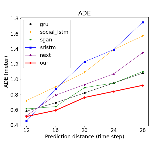
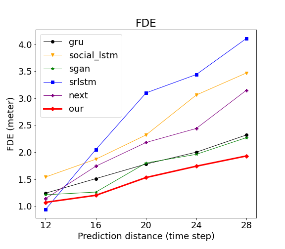
Figure 5: Performance of compared models in ADE - left and FDE - right (the lower the better) on ranging prediction length. GTP (red diamond) shows increasingly favorable performance over baselines while other state-of-the-art only have the advantage in short-range prediction. Detailed numeric results are included in the supplementary materials.

Different from other RNN based future predictors [25, 31], both of GTP’s channels rely heavily on the personalized perception of each pedestrian about the destinations. Although the network could learn to adapt the geometrical relationship in any reference frames, we want it to concentrate on modeling the relative perception of goals and trajectory rather than the absolute scale of the scenes. For that purpose, we represent both the trajectory and the destinations’ geometrical features in the personalized coordinate system with respect to each pedestrian called the agent-centric coordinate (see Fig. 4).

These coordinates is defined to be rooted at $q_{t_{obs}}$ and has the unit vector $\overrightarrow{u}=(-1,0)$ transformed from $\overrightarrow{q_{t_{obs}}q_{1}}$. All parts of the trajectory including observed $X$ and predicted $Y$ are transformed to this system before being used in GTP.

Under the agent-centric coordinate, the destination features $d_{i}$ includes the relative distance and direction of the destination in the perspective of the pedestrian:

$$d_{i}=(x_{min_{i}},y_{min_{i}},x_{max_{i}},y_{max_{i}},\theta_{min_{i}},\theta_{max_{i}}),$$

where the first four elements are the coordinate of the destination regions and the last two represent angle ranges from pedestrian’s point of view.

Experimental results showing the effective of this representation is detailed in the ablation study (Sec. IV-E)

III-E Training GTP

When training the model, we need to attain the balance and collaboration between optimizing the Goal channel loss $\mathcal{L}_{g}$ and the Trajectory channel loss $\mathcal{L}_{tr}$. To this end, we use a three-stage training process. At the first stage, we fix the Trajectory channel and only train Goal channel with $\mathcal{L}_{g}$ to ensure that the modulated destinations $E$ capture goal-related information. Then, in the second stage, we freeze the Goal channel, keeping the modulated representations $E$ unchanged, and train Trajectory channel with $\mathcal{L}_{tr}$. Finally, in the last stage, we refine the whole model using $\mathcal{L}_{tr}$.

IV Experiments

(a)

(b)

Figure 6: Qualitative analysis of GTP. (a) GRU predicts the pedestrian to follow the upward trend in the observed trajectory, while GTP estimates the destination to be Goal 5 and generates trajectory toward that destination. (b) Similarly, the correct estimated goal (Goal 7) enable GTP to perform better than simple GRU. We provide more cases in supplementary materials.

IV-A Experiment Settings

Dataset

We use the two most prominent benchmark datasets for trajectory predictions which are ETH [20] and UCY [17]. These datasets contain real-world annotated trajectories in five different scenes: ETH, HOTEL (from ETH dataset), ZARA1, ZARA2, UNIV (from UCY dataset). Similar to previous works [1, 10, 18, 31], we preprocess the trajectories to convert from camera coordinates to world coordinates using provided homography parameters.

Baselines

We compare our method against four state-of-the-art methods Social LSTM [1], Social GAN [10], SR-LSTM [31] and Next [18]. We also use a baseline GRU Encoder-Decoder, which is the base architecture that all of these works developed on top of.

Evaluation protocols and metrics

The common setting used in the state-of-the-arts is observing 8 time steps (3.2 seconds) and predict the near-term future trajectories in the next 12 time steps (4.8 seconds). With the objective of long-term prediction, we extend this setting into maximal future distance possible supported by the dataset. This results in the settings of observing 8 and predicting 12, 16, 20, 24, 28 time steps. For all of the methods, a model for each of these settings is trained separately.

As with other methods, we use the leave-one-out cross-validation approach, training on 4 scenes, and testing on the remaining unseen scene. The performance is measured using two error metrics: Average displacement error (ADE) and Final displacement error (FDE).

In reporting results, we cite the results reported in the baseline papers when possible. In the new settings of far-term prediction, we retrain these models using the standard published implementation.

IV-B Quantitative Performances

The performance of GTP and other methods are graphed in Figure 5. It showed that some of the state-of-the-art methods, namely SR-LSTM [31] and Next [18] have advantages over baseline GRU only in the short-term 12 time-step prediction. However, all of these methods have fast deteriorating performances along with prediction distances.

By contrast, GTP’s performances are much more stable in the far-term prediction. Although the model is slightly worse than SR-LSTM in 12 time steps prediction, it outperforms all of the baselines in other prediction settings. Also, the farther the prediction is, the gap between GTP and other methods getting more and more widened.

The strong performance of GTP in far-term prediction could be attributed to the collaborative interaction between the two channels. By considering the modulated representations $E=(e_{1},...,e_{n_{dest}})$ provided by Goal Channel, Trajectory Channel has access to the possible goals of the pedestrian; therefore, the model could generate consistent future locations toward the correct destination. By contrast, baseline models are unaware of the goal concept and only use the immediate continuity of the trajectory. Without the long-term guidance, the recurrent predictors accumulate the errors in each step, leading to plummeted performance.

IV-C Qualitative Analysis

We further investigate the dependence of future trajectories on goals by visualizing the results generated from GTP and GRU baseline. As shown in Figure 6, GRU could only predict future trajectories based on the dynamic of the observed trajectory, and hence it will fail when the moving pattern is complex. Certainly, in Figure 6a, GRU predicts the pedestrian to follow his upward trend, while the true trajectory is to move forward. By contrast, GTP predicts that the pedestrian will reach Goal 5 and generate future positions toward that destination. Similarly, in Figure 6b, the estimated goal enable GTP to predict accurate trajectory, which could not be achieved in simple GRU.

#		obs8 - pred12	obs8 - pred16	obs8 - pred20	obs8 - pred24	obs8 - pred28
0	Full GTP model	0.51 / 1.07	0.59 / 1.20	0.76 / 1.53	0.84 / 1.74	0.92 / 1.93
1	W/o destination modulation	0.52 / 1.09	0.65 / 1.37	0.86 / 1.82	1.23 / 2.67	1.24 / 2.77
2	W/o goal loss	0.50 / 1.06	0.60 / 1.24	0.78 / 1.61	0.92 / 1.94	1.07 / 2.30
3	W/o flexible attention weights	0.51 / 1.07	0.62 / 1.3	0.76 / 1.57	0.88 / 1.84	0.99 / 2.09
4	W/o agent-centric coordinates	0.6 / 1.28	0.68 / 1.46	0.81 / 1.76	0.96 / 2.05	1.01 / 2.12
5	W/o any goal-driven features	0.58 / 1.24	0.69 / 1.51	0.82 / 1.78	0.95 / 2.0	1.08 / 2.32

TABLE I: Ablation experiments for trajectory prediction in ADE/FDE. The lower the numbers, the better the model.

IV-D Model Behavior Analysis

To have a better view of how the Trajectory channel uses the modulated destinations $E$, we visualize the attention weights $\alpha_{ti}$ in ctr block in several cases (see Figure 7).

In the first example (Fig. 7a), the ctr block initially paid the most attention to destination 3 and 6 and gave uniform weights to the rest. As the prediction progressed, it gradually concentrated more on destination 2 and 9 as they became potential goal choices.

In the second example (Fig. 7b), at the early stage, ctr considered destination 2 the most. However, at the later stage, as the trajectory progressed from right to left, destination 2 is no longer the most potential candidate, it switched to considering the information contained in the potential goals in destinations 1, 4, 5, and 7. The attention weights of these short-listed destinations got sharper and sharper attention as the probable goal choices narrowed.

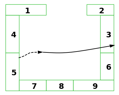
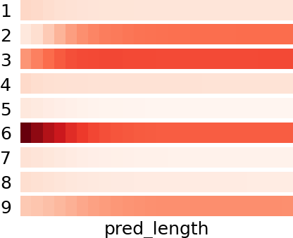
(a)

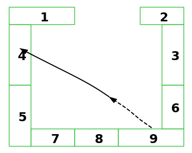
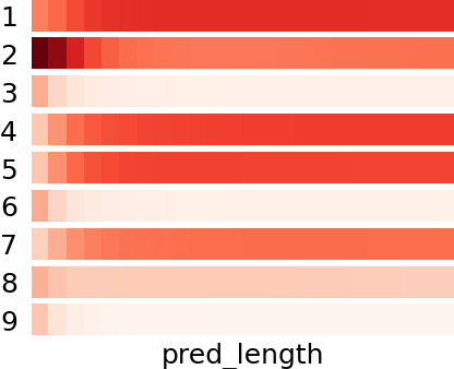
(b)

Figure 7: Patterns of attention weights used in ctr block as trajectory prediction progresses. The farther toward the end, the sharper attention was put on narrowed down choices among the destinations.

IV-E Ablation Study

We provide more insight about the roles of GTP components and choices by turning off each of the key proposed components. The results of the study are reported in Table I.

1. Without destination modulation. We investigate the contribution of modulated representations by ablating them from the model. Specifically, in the third row of Table I, we use the raw destination representations $D$, instead of the modulated representations $E$, to compute the controlling signal in Eq. 10, 11. The results show that using raw destination features is better than not using them at all (row 1 vs row 5). However, modulating those features by the Goal channel helps GTP reaches its maximum advantages (row 0).

2. Without goal loss. Without using the goal loss, there is no guarantee that the modulated representations contain goal-related information. Consequently, the performances of GTP in long-term prediction (20 to 28 time-steps) decrease significantly.

3. Without flexible attention weights. In this experiment, we test the straightforward alternative of directly using the ranking scores $r_{i}$ of the Goal channel (Eq. 7) in place of $\alpha_{ti}$ to compute the controlling signal $c_{t}$ in Eq. 11; by doing this, we bypass the computation of attention weights $\alpha_{ti}$ at every time step. Although saving some computation, this rigid option does not allow attention to adapt to the evolving situation; hence, it leads to a reduction in performance, especially in far-terms.

4. Without agent centric coordinates. Using the raw world coordinates hurts the performance of GTP significantly. This indicates that agent-centric coordinate plays an important role in estimating and utilizing agent’s goal information.

5. Without any goal-driven features. This model is equivalent to a vanilla GRU encoder-decoder baseline. It is clear that most of the proposed features make improvements over this baseline; and combination of these features in the full GTP model leads to the best result.

V Conclusion

In this work, we study the problem of forecasting human trajectory into the far future. We propose GTP: a dual-channel network for jointly modeling the goals and trajectory of pedestrians. Through experiments, we have verified that GTP effectively takes advantage of the imposed goal structures and provides strong consistency in long-term prediction, and reduces the progressive accumulation of error.

This work opens room for future investigations on considering long-term goals together with the short-term social and environmental context. Static environmental factors can be incorporated easily into the input at each step. Social interaction can be introduced through message passing between trajectory channels and shared goal modeling.

References

- [1] Alexandre Alahi, Kratarth Goel, Vignesh Ramanathan, Alexandre Robicquet, Li Fei-Fei, and Silvio Savarese. Social lstm: Human trajectory prediction in crowded spaces. In Proceedings of the IEEE conference on computer vision and pattern recognition, pages 961–971, 2016.
- [2] Javad Amirian, Jean-Bernard Hayet, and Julien Pettré. Social ways: Learning multi-modal distributions of pedestrian trajectories with gans. In Proceedings of the IEEE Conference on Computer Vision and Pattern Recognition Workshops, pages 0–0, 2019.
- [3] Niccoló Bisagno, Bo Zhang, and Nicola Conci. Group lstm: Group trajectory prediction in crowded scenarios. In Proceedings of the European conference on computer vision (ECCV), pages 0–0, 2018.
- [4] Ennio Cascetta. Random utility theory. In Transportation systems analysis, pages 89–167. Springer, 2009.
- [5] Ming-Fang Chang, John Lambert, Patsorn Sangkloy, Jagjeet Singh, Slawomir Bak, Andrew Hartnett, De Wang, Peter Carr, Simon Lucey, Deva Ramanan, et al. Argoverse: 3d tracking and forecasting with rich maps. In Proceedings of the IEEE Conference on Computer Vision and Pattern Recognition, pages 8748–8757, 2019.
- [6] Bang Cheng, Xin Xu, Yujun Zeng, Junkai Ren, and Seul Jung. Pedestrian trajectory prediction via the social-grid lstm model. The Journal of Engineering, 2018(16):1468–1474, 2018.
- [7] Chiho Choi, Abhishek Patil, and Srikanth Malla. Drogon: A causal reasoning framework for future trajectory forecast. arXiv preprint arXiv:1908.00024, 2019.
- [8] Junyoung Chung, Caglar Gulcehre, KyungHyun Cho, and Yoshua Bengio. Empirical evaluation of gated recurrent neural networks on sequence modeling. arXiv preprint arXiv:1412.3555, 2014.
- [9] Maurizio Corbetta and Gordon L Shulman. Control of goal-directed and stimulus-driven attention in the brain. Nature reviews neuroscience, 3(3):201–215, 2002.
- [10] Agrim Gupta, Justin Johnson, Li Fei-Fei, Silvio Savarese, and Alexandre Alahi. Social gan: Socially acceptable trajectories with generative adversarial networks. In Proceedings of the IEEE Conference on Computer Vision and Pattern Recognition, pages 2255–2264, 2018.
- [11] Sepp Hochreiter and Jürgen Schmidhuber. Long short-term memory. Neural computation, 9(8):1735–1780, 1997.
- [12] Ashesh Jain, Amir R Zamir, Silvio Savarese, and Ashutosh Saxena. Structural-rnn: Deep learning on spatio-temporal graphs. In Proceedings of the ieee conference on computer vision and pattern recognition, pages 5308–5317, 2016.
- [13] Vasiliy Karasev, Alper Ayvaci, Bernd Heisele, and Stefano Soatto. Intent-aware long-term prediction of pedestrian motion. In 2016 IEEE International Conference on Robotics and Automation (ICRA), pages 2543–2549. IEEE, 2016.
- [14] Kris M Kitani, Brian D Ziebart, James Andrew Bagnell, and Martial Hebert. Activity forecasting. In European Conference on Computer Vision, pages 201–214. Springer, 2012.
- [15] Vineet Kosaraju, Amir Sadeghian, Roberto Martín-Martín, Ian Reid, Hamid Rezatofighi, and Silvio Savarese. Social-bigat: Multimodal trajectory forecasting using bicycle-gan and graph attention networks. In Advances in Neural Information Processing Systems, pages 137–146, 2019.
- [16] Namhoon Lee, Wongun Choi, Paul Vernaza, Christopher B Choy, Philip HS Torr, and Manmohan Chandraker. Desire: Distant future prediction in dynamic scenes with interacting agents. In Proceedings of the IEEE Conference on Computer Vision and Pattern Recognition, pages 336–345, 2017.
- [17] Alon Lerner, Yiorgos Chrysanthou, and Dani Lischinski. Crowds by example. In Computer graphics forum, volume 26, pages 655–664. Wiley Online Library, 2007.
- [18] Junwei Liang, Lu Jiang, Juan Carlos Niebles, Alexander G Hauptmann, and Li Fei-Fei. Peeking into the future: Predicting future person activities and locations in videos. In Proceedings of the IEEE Conference on Computer Vision and Pattern Recognition, pages 5725–5734, 2019.
- [19] Matteo Lisotto, Pasquale Coscia, and Lamberto Ballan. Social and scene-aware trajectory prediction in crowded spaces. In Proceedings of the IEEE International Conference on Computer Vision Workshops, pages 0–0, 2019.
- [20] Stefano Pellegrini, Andreas Ess, Konrad Schindler, and Luc Van Gool. You’ll never walk alone: Modeling social behavior for multi-target tracking. In 2009 IEEE 12th International Conference on Computer Vision, pages 261–268. IEEE, 2009.
- [21] Eike Rehder and Horst Kloeden. Goal-directed pedestrian prediction. In Proceedings of the IEEE International Conference on Computer Vision Workshops, pages 50–58, 2015.
- [22] Eike Rehder, Florian Wirth, Martin Lauer, and Christoph Stiller. Pedestrian prediction by planning using deep neural networks. In 2018 IEEE International Conference on Robotics and Automation (ICRA), pages 1–5. IEEE, 2018.
- [23] Andrey Rudenko, Luigi Palmieri, and Kai O Arras. Joint long-term prediction of human motion using a planning-based social force approach. In 2018 IEEE International Conference on Robotics and Automation (ICRA), pages 1–7. IEEE, 2018.
- [24] Andrey Rudenko, Luigi Palmieri, Michael Herman, Kris M Kitani, Dariu M Gavrila, and Kai O Arras. Human motion trajectory prediction: A survey. The International Journal of Robotics Research, 39(8):895–935, 2020.
- [25] Amir Sadeghian, Vineet Kosaraju, Ali Sadeghian, Noriaki Hirose, Hamid Rezatofighi, and Silvio Savarese. Sophie: An attentive gan for predicting paths compliant to social and physical constraints. In Proceedings of the IEEE Conference on Computer Vision and Pattern Recognition, pages 1349–1358, 2019.
- [26] Charlie Tang and Russ R Salakhutdinov. Multiple futures prediction. In Advances in Neural Information Processing Systems, pages 15424–15434, 2019.
- [27] Daksh Varshneya and G Srinivasaraghavan. Human trajectory prediction using spatially aware deep attention models. arXiv preprint arXiv:1705.09436, 2017.
- [28] Anirudh Vemula, Katharina Muelling, and Jean Oh. Social attention: Modeling attention in human crowds. In 2018 IEEE international Conference on Robotics and Automation (ICRA), pages 1–7. IEEE, 2018.
- [29] Yanyu Xu, Zhixin Piao, and Shenghua Gao. Encoding crowd interaction with deep neural network for pedestrian trajectory prediction. In Proceedings of the IEEE Conference on Computer Vision and Pattern Recognition, pages 5275–5284, 2018.
- [30] Hao Xue, Du Q Huynh, and Mark Reynolds. Ss-lstm: A hierarchical lstm model for pedestrian trajectory prediction. In 2018 IEEE Winter Conference on Applications of Computer Vision (WACV), pages 1186–1194. IEEE, 2018.
- [31] Pu Zhang, Wanli Ouyang, Pengfei Zhang, Jianru Xue, and Nanning Zheng. Sr-lstm: State refinement for lstm towards pedestrian trajectory prediction. In Proceedings of the IEEE Conference on Computer Vision and Pattern Recognition, pages 12085–12094, 2019.
- [32] Tianyang Zhao, Yifei Xu, Mathew Monfort, Wongun Choi, Chris Baker, Yibiao Zhao, Yizhou Wang, and Ying Nian Wu. Multi-agent tensor fusion for contextual trajectory prediction. In Proceedings of the IEEE Conference on Computer Vision and Pattern Recognition, pages 12126–12134, 2019.
- [33] Stephan Zheng, Yisong Yue, and Jennifer Hobbs. Generating long-term trajectories using deep hierarchical networks. In Advances in Neural Information Processing Systems, pages 1543–1551, 2016.
- [34] Bolei Zhou, Hang Zhao, Xavier Puig, Sanja Fidler, Adela Barriuso, and Antonio Torralba. Scene parsing through ade20k dataset. In Proceedings of the IEEE Conference on Computer Vision and Pattern Recognition, 2017.
- [35] Bolei Zhou, Hang Zhao, Xavier Puig, Tete Xiao, Sanja Fidler, Adela Barriuso, and Antonio Torralba. Semantic understanding of scenes through the ade20k dataset. International Journal on Computer Vision, 2018.
- [36] Brian D Ziebart, Nathan Ratliff, Garratt Gallagher, Christoph Mertz, Kevin Peterson, J Andrew Bagnell, Martial Hebert, Anind K Dey, and Siddhartha Srinivasa. Planning-based prediction for pedestrians. In 2009 IEEE/RSJ International Conference on Intelligent Robots and Systems, pages 3931–3936. IEEE, 2009.