Variations of helioseismic parameters due to magnetic field generated by a flux transport model

Abstract

The change of sound speed has been found at the base of the convection during the solar cycles, which can be used to constrain the solar internal magnetic field. We aim to check whether the magnetic field generated by the solar dynamo can lead to the cyclic variation of the sound speed detected through helioseismology. The basic configuration of magnetic field in the solar interior was obtained by using a Babcock-Leighton (BL) type flux transport dynamo. We reconstructed one-dimensional solar models by assimilating magnetic field generated by an established dynamo and examined their influences on the structural variables. The results show that magnetic field generated by the dynamo is able to cause noticeable change of the sound speed profile at the base of the convective zone during a solar cycle. Detailed features of this theoretical prediction are also similar to those of the helioseismic results in solar cycle 23 by adjusting the free parameters of the dynamo model.

1 Introduction

Helioseimology has been regarded as a powerful tool to detect the properties of the solar interior that are not directly observed (Christensen-Dalsgaard et al., 1996). Global helioseimology utilizes the normal modes of oscillation of the Sun to determine the interior structure and dynamics. The oscillation frequencies are known to vary on timescales related to the solar cycles (e.g., Woodard & Noyes, 1985; Libbrecht & Woodard, 1990; Elsworth et al., 1990; Basu & Schou, 2000; Howe et al., 2000). The change of frequency has been shown to be highly correlated with surface activity (e.g., Chaplin et al., 2007; Jain et al., 2009; Broomhall et al., 2009; Tripathy et al., 2015; Howe et al., 2018). They concluded that the observed frequency change is confined to the shallow layer of the Sun. In addition, Howe et al. (2002) showed that the temporal and latitudinal distribution of the frequency shifts is correlated with the distribution of the surface magnetic field.

With improved data and analysis techniques in recent years, helioseimology has successfully probed the structural changes in the deeper layers of the convective zone, especially the tachocline at the base of the convective zone. Although the solar oscillation frequencies have been determined with tremendous precision, statistical errors in those frequencies are still too large to make any direct detections of structural change in the deep interior. Two major approaches were suggested to meet these challenges. One is to use the smoothed and scaled frequency change as a function of the lower turning point (Chou & Serebryanskiy, 2005; Serebryanskiy & Chou, 2005). The other one is to use a principal component analysis (PCA) method to separate the frequency differences into a linear combination of different time-dependent components (Baldner & Basu, 2008). In both cases, a small but statistically significant change in the sound speed with an origin at and below the base of the convection zone was found. By assuming that the entire change is due to the presence of magnetic field, they constrained a magnetic field strength in the order of $\sim 10^{5}$G. Baldner & Basu (2008) and Baldner et al. (2009) also showed that the sound speed inversions are tightly correlated with the latitudinal distribution of surface activity. Besides, Liang & Chou (2015) presented the travel time difference which was attributed to the change of magnetic field. Therefore, combining the observed sound speed variation with the frequency shift would provide more constraints on the configuration of the magnetic field deep inside the Sun.

It is widely accepted that all the solar activities are dominated by the solar magnetic field generated inside the Sun due to the dynamo process. Where the magnetic field is generated and how the magnetic field is distributed are longstanding and outstanding questions in solar physics. Up to date, a number of dynamo models have been developed for investigating the dynamo process. The details of models can be found in the reviews by Charbonneau (2010, 2014). Global MHD simulation of the solar convective zone is the most direct way to tackle the solar convective zone. Simulations of convection-driven dynamos have recently reached a level of sophistication (Hotta et al., 2016; Strugarek et al., 2017). However, due to a wide range of spatial and temporal scales characterizing the solar convection, the variability seen in the simulations is not directly comparable to that of the Sun. The kinematic flux transport dynamo (FTD) model based on the Babcock-Leighton (BL) mechanism, which was first proposed by Babcock (1961) and further elaborated by Leighton (1964), is regarded as one of the most promising models in understanding the solar cycle during the past several years (e.g., Jiang et al., 2007; Cameron et al., 2010; Jiang et al., 2013). Thanks to the fundamental works of Nandy & Choudhuri (2002) and Chatterjee et al. (2004), the code SURYA based on the FTD model has been well developed and open to the public for years (Choudhuri, 2017).

With the variable magnetic field and turbulence included, one-dimensional models of the structure and evolution of the Sun were constructed, which were then compared to observations (Li et al., 2003). Since the magnetic configuration is unknown, Li et al. (2003) assumed a Gaussian profile of the magnetic field concentrated at different depths with different amplitudes. They found a model with magnetically modulated turbulence which reproduces shifts of oscillation frequencies observed in the solar cycle 23. This result, however, contains an obvious limitation. That is the simple descriptions of magnetic field during a solar cycle: a Gaussian distribution below the surface with varying amplitude. Therefore, we aim to develop the solar variability model field, e.g., those generated by the FTD models. Different from Li et al. (2003), this work will focus on the structural variations at the tachocline where strong magnetic field is generated.

In this work, we adopted the code SURYA to generate generate a series of magnetic profiles through a complete solar cycle, and then incorporate the self-consistent magnetic fields into the computation of stellar evolution models for investigating the effects of the magnetic fields on the structural properties and the oscillation frequencies. In Section 2, we describe the physical ingredients of the dynamo model and the solar variability model. Section 3 presents the details of the magnetic profiles generated by a FTD model in a complete solar cycle. In Section 4, we show the impacts on the solar internal structural variables due to magnetic field. The discussions and conclusions are given in Section 5.

2 Theoretical Models

In this section, we briefly introduce the physical ingredients for a BL type flux transport dynamo model, and for a solar variability model that includes the effects of magnetic field and rotation.

2.1 The Flux Transport Dynamo Model

Solar magnetic activity involves the generation and evolution of magnetic field. The important ingredients in the flux transport dynamo model are as follows. (1) The strong toroidal field is produced by stretching of the poloidal field lines, which is caused by the differential rotation within the tachocline where the rotational velocity sharply changes with depth and latitude; (2) When the toroidal field $B_{\rm t}$ exceeds the critical field value $B_{\rm c}$, the tachocline toroidal field undergo buoyant rise through the convection zone to produce sunspots; (3) the poloidal field can be generated by the BL process; (4) The meridional circulation plays an important role for the advection of the toroidal and poloidal field (Chatterjee et al., 2004; Jiang et al., 2007; Choudhuri, 2020).

In the spherical polar coordinates $\left(r,\theta,\phi\right)$, the averaged large-scale magnetic field and plasma flow under the assumption of axisymmetry about the Sun’s rotation axis, can be expressed as

$$\mathbf{B}=B_{\rm t}\left(r,\theta\right)\mathbf{e}_{\phi}+\nabla\times\left[A\left(r,\theta\right)\bf{e}_{\phi}\right],$$ (1)

$$\mathbf{v}=\Omega\left(r,\theta\right)r\sin\theta\mathbf{e}_{\phi}+\mathbf{v}_{\rm p},$$ (2)

where $\mathbf{B}_{\rm t}=B_{\rm t}\left(r,\theta\right)\mathbf{e}_{\phi}$, $\mathbf{B}_{\rm p}=\nabla\times\left[A\left(r,\theta\right)\mathbf{e}_{\phi}\right]$ are the toroidal field and poloidal field, respectively. The first term of equation (2) denotes the $\phi$-component of the velocity, i.e., angular velocity $\Omega(r,\theta)$ of the solar interior inferred from helioseismic data (Kosovichev, 1996; Schou et al., 1998), while $\mathbf{v}_{\rm p}={\rm v}_{\rm r}(r,\theta)\mathbf{e}_{\rm r}+{\rm v}_{\theta}(r,\theta)\textbf{e}_{\theta}$ is the meridional circulation. The equations for the standard $\alpha\Omega$ dynamo model are given as follows:

$$\frac{\partial A}{\partial t}=\eta_{\rm p}\left(\nabla^{2}-\frac{1}{s^{2}}\right)A-\frac{1}{s}\left(\mathbf{v}_{\rm p}\cdot\nabla\right)\left(sA\right)+\alpha B_{\rm t},$$ (3)

$$\frac{\partial B_{\rm t}}{\partial t} = \eta_{\rm t}\left(\nabla^{2}-\frac{1}{s^{2}}\right)B_{\rm t}+\frac{1}{r}\frac{d\eta_{\rm t}}{dr}\frac{\partial}{\partial r}\left(rB_{\rm t}\right)$$

$$- \frac{1}{r}\left[\frac{\partial}{\partial r}\left(r{\rm v}_{\rm r}B_{\rm t}\right)+\frac{\partial}{\partial\theta}\left({\rm v}_{\theta}B_{\rm t}\right)\right]+s\left(\mathbf{B}_{\rm p}\cdot\nabla\right)\Omega,$$

where $s=r\sin\theta$. The turbulence diffusion coefficients $\eta_{\rm p}$ and $\eta_{\rm t}$ correspond to the poloidal and toroidal components, respectively. The coefficient $\alpha$ expresses a BL source term which describes the generation of poloidal field due to the buoyant eruption and flux dispersal of tilted active regions.

Here we describe a few key parameters in particular. The meridional flow plays essential roles in the BL type dynamo. It dominates the cycle period and is mainly responsible for the equatorward migration of the toroidal field and poleward migration of the poloidal field on the solar surface. It is noted that the penetration depth and the number of circulation cells are still the subjects of hot debate. We follow Chatterjee et al. (2004) to adopt a deep penetrated one-cell meridional flow. It goes slightly below the tachocline until $0.61R_{\odot}$. A strong turbulent diffusivity $\eta_{p}=2.6\times 10^{12}$ cm² s^-1 is adopted for the poloidal field, which corresponds to the diffusion-dominated flux transport dynamos. This distinguishes from the advection-dominated ones with low turbulent diffusivity. The different strength of $\eta_{p}$ has large effects on the path of the flux transport and flux structure in the convective zone. The $\alpha$-effect is concentrated in the top layer $0.95R_{\odot}\leq r\leq R_{\odot}$ , where $\alpha$ changes with latitude as $\cos\theta$. The only nonlinear suppression of the magnetic field growth is provided by magnetic buoyancy. The magnetic buoyancy is dealt in the same way as Chatterjee et al. (2004). A critical field $B_{c}$ is set. Wherever the toroidal field $B$ exceeds $B_{c}$, a fraction $f$ = 0.5 of the magnetic flux is assumed to erupt to the surface layers, with the toroidal field values adjusted appropriately to ensure flux conservation. The rest part of the dynamo system is linear. The adopted value of $B_{c}$ sets the magnetic field scale of the solutions. It will be an adjustable parameter in Section 3 to make a constraint on the possible field strength in the convective zone. The widely studied parameters, such as turbulent pumping, are not included in the model (Jiang et al., 2013).

The axisymmetric dynamo equations (3) and (4) are to be solved in a meridional slab, i.e., $R_{\rm b}\leq r\leq R_{\odot}$ and $0\leq\theta\leq\pi$, with the inner boundary at $R_{\rm b}=0.55R_{\odot}$. Assuming a perfectly conducting solar core, at the inner radius $(r=R_{b})$, or at the poles $(\theta=0,\pi)$, we have

$$A=0,\ \ \ B_{t}=0.$$ (5)

In general, it is assumed that the Sun is in a vacuum without electrical currents, i.e., $\nabla\times\textbf{B}=0$. At the top $\left(r=R_{\odot}\right)$, the toroidal field has to be zero and the poloidal field has to match smoothly a potential field satisfying the free space equation, this requires

$$\left(\nabla^{2}-\frac{1}{r^{2}\sin^{2}\theta}\right)A=0,\ \ \ B_{t}=0.$$ (6)

The wider radial region of our calculated spherical shell compared to other models, which are usually in the range of $\left(0.65R_{\odot},1.0R_{\odot}\right)$, makes the comparisons with the helioseismologic results more feasible.

2.2 1-D Solar Models with Magnetic field

When the influence of a cyclic magnetic field is considered, the solar models become variable (see Li et al., 2003). Cyclic magnetic field $\mathbf{B}$, given by the flux transport dynamo model, is a vector with two components. Within the framework of 1-D stellar evolution model, instead of using the two components, new variables were introduced to the stellar basic equations, namely, the magnetic energy per unit mass $\chi$ and magnetic field direction $\gamma$, which are defined as (Lydon & Sofia, 1995):

$$\chi=(B^{2}/8\pi)/\rho,\ \ \ \gamma=1+B^{2}_{\rm t}/B^{2},$$ (7)

where $B^{2}=B^{2}_{\rm t}+B^{2}_{\rm p}$.

Following Li & Sofia (2001) and Li et al. (2003), the stellar structure variables, $\chi$ and $\gamma$, can be used to describe the magnetic structure of a star in the one-dimensional stellar modeling. The magnetic pressure $P_{\rm m}$ can be defined as:

$$P_{\rm m}=(\gamma-1)\chi\rho.$$ (8)

The equation of state is modified as $\rho=\rho\left(P,T,\chi,\gamma\right)$, and the corresponding differential form is given by

$$\frac{d\rho}{\rho}=\zeta\frac{dP}{P}-\delta\frac{dT}{T}-\lambda\frac{d\chi}{\chi}-\mu\frac{d\gamma}{\gamma}.$$ (9)

The first law of thermodynamics should be written as

$$TdS = dU+PdV-d\chi,$$

$$= c_{P}dT-\frac{\delta}{\rho}dP+\left(\frac{P\delta\lambda}{\rho\zeta\chi}-1\right)d\chi+\frac{P\delta\mu}{\rho\zeta\gamma}d\gamma,$$

where the total pressure is defined as $P=P_{0}+P_{\rm m}$, and $P_{0}$ is the gas pressure. The related derivatives are

$$\zeta=\left(\frac{\partial\ln\rho}{\partial\ln P}\right)_{\rm T,\chi,\gamma},\ \ \delta=-\left(\frac{\partial\ln\rho}{\partial\ln T}\right)_{\rm P,\chi,\gamma},$$

$$\lambda=-\left(\frac{\partial\ln\rho}{\partial\ln\chi}\right)_{\rm P,\rm T,\gamma},\ \ \mu=-\left(\frac{\partial\ln\rho}{\partial\ln\gamma}\right)_{\rm P,\rm T,\chi}.$$

A detailed derivation of the solar variable model, which includes the effect of magnetic field, was described in Lydon & Sofia (1995) and Li & Sofia (2001).

Consequently, when magnetic field and rotation are included, the stellar structure equations are modified by the following (Denissenkov & Pinsonneault, 2007; Eggenberger et al., 2008)

$$\frac{\partial P}{\partial M_{\rm P}} = -\frac{GM_{\rm P}}{4\pi r_{\rm P}^{4}}f_{\rm P},$$ (11)

$$\frac{\partial r_{\rm P}}{\partial M_{\rm P}} = \frac{1}{4\pi r_{\rm P}^{2}\rho},$$ (12)

$$\frac{\partial L_{\rm P}}{\partial M_{\rm P}} = \epsilon-T\frac{dS}{dt},$$ (13)

$$\frac{\partial T}{\partial M_{\rm P}} = -\frac{GM_{\rm P}}{4\pi r_{\rm p}^{4}}f_{\rm P}\min\left[\nabla_{\rm con},\nabla_{\rm rad}\frac{f_{\rm T}}{f_{\rm P}}\right],$$ (14)

where the subscript $P$ refers to the isobar value. The nondimensional rotating corrective factors $f_{\rm P}$ and $f_{\rm T}$ depend on the shape of the isobars, namely

$$f_{\rm P}=-\frac{4\pi r_{\rm p}^{4}}{GM_{\rm P}S_{\rm P}}\frac{1}{\langle g^{-1}\rangle},\\$$

$$f_{\rm T}=\left(\frac{4\pi r_{\rm p}^{2}}{S_{\rm P}}\right)^{2}\frac{1}{\langle g\rangle\langle g^{-1}\rangle}.$$

Here $\langle g\rangle$ and $\langle g^{-1}\rangle$ are the mean values of the effective gravity and its inverse over the equipotential surface. $S_{\rm p}$ is the surface area of the equipotential, while other variables have been described by Meynet & Maeder (1997).

3 Magnetic field generated by FTD models

In this section, we demonstrate the details of the magnetic field generated by a FTD model (SUYRA) in a complete solar cycle and how we transform magnetic field from 2-D to 1-D for assimilating them into a solar model. We generated a series of magnetic profiles with SURYA. There are three adjusted input parameters and we set up them following Chatterjee et al. (2004). Magnetic buoyancy is prescribed in the way that the toroidal field exceeding the critical field $B_{c}$ is searched above the base of convective zone taken at $r$ = 0.71. Wherever the magnetic strength exceeds $B_{c}$, a fraction of $f$ = 0.5 of it is made to erupt to the surface layers, with the toroidal field values adjusted appropriately to ensure flux conservation. We refer this dynamo model as the SURYA Standard Case in the following analysis. Figure 1 shows the butterfly diagram of eruptions when $B_{c}$ is equal to $2\times 10^{5}$ G. The solid and dashed lines are the contours of the radial field. The sunspot eruptions are confined within $\pm 40^{\circ}$ and the butterfly diagrams have shapes similar to observations. The weak radial field migrates poleward at higher latitudes. The phase relation between the sunspots and the weak diffuse field is also produced. All of these are consistent with the observed magnetic butterfly diagram.

Figure 1: Theoretical butterfly diagram of eruptions for the simulation given by SURYA. The time and latitude of eruption for toroidal field are denoted by crosses. The solid and dashed lines are the contours of diffuse radial field. The dashed contours are for negative $B_{\rm r}$, and the solid contours are for positive $B_{\rm r}$.

Figure 2 displays the 2-D distribution of the toroidal field in red and blue colors and the poloidal field in solid and dashed curves at an interval of 1/6 the solar cycle period in the first half of one solar cycle, ordered from the minimum to the maximum. As presented in Jiang et al. (2007), the poloidal field is radially transported to the bottom of the convective zone under the effect of strong turbulent diffusion and is poleward transported to the pole due to the effect of poleward meridional flow simultaneously. The arrival of the poloidal field changes the strength of the toroidal field. The toroidal field distribution is also affected by the transport of the deep penetrated meridional flow. The strong effects of the meridional flow and the radial shear at the base of the convective zone cause the multi structures and evolution of the toroidal field around 0.6-$0.7R_{\odot}$.

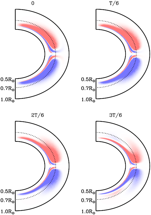
Figure 2: Theoretical distribution of toroidal magnetic field generated by a BL type flux transport dynamo model. Positive $B_{\rm t}$ is showed in blue, and negative $B_{\rm t}$ is plotted in red.

For a 1-D stellar evolution model, the time series of 2-D magnetic field has been converted into 1-D data. As demonstrated in Figure 2, the most magnetic activities appear at low and middle latitudes, hence we focus on a belt region from equator to $45^{\circ}$. The toroidal magnetic field distributed at nine latitude regions, i.e., $5^{\circ}\pm 2.5^{\circ}$, $10^{\circ}\pm 2.5^{\circ}$, $15^{\circ}\pm 2.5^{\circ}$, $20^{\circ}\pm 2.5^{\circ}$, $25^{\circ}\pm 2.5^{\circ}$, $30^{\circ}\pm 2.5^{\circ}$, $35^{\circ}\pm 2.5^{\circ}$, $40^{\circ}\pm 2.5^{\circ}$ and $45^{\circ}\pm 2.5^{\circ}$, are picked up and averaged individually as 1-D data. These 1-D data are assimilated in the 1-D solar model one at a time. Subsequently, we study the effects of magnetic field at one latitude region. Note that this is a simple and rough approximation and turns out to be the major limitation of this approach. Because the purpose of this work is to investigate the changes caused by magnetic field, we hence care the differences of magnetic strength rather than the absolute value. Figure 3 shows the radial distributions of the magnetic field difference between solar minimum and maximum. The four panels correspond to four latitudes., i.e., 5^∘, 15^∘, 30^∘, and 45^∘. As is shown that, the major changes are located below the base of convection zone, and no noticeable difference appears above 0.8$R_{\odot}$. This is because the SUYRA code does not consider a second dynamo near the surface. Since this work focuses on the helioseismic signals at the tachocline, the dynamo model is adequate.

Figure 3: The changes in magnetic profiles between the minimum and the maximum of the SUYRA Standard Case at separated latitudes ($5^{\circ}$, $15^{\circ}$, $30^{\circ}$ and $45^{\circ}$).

4 Structural Variations in the solar interior

The solar model we use in this paper is an established one obtained by Bi et al. (2011). The model was calculated by the one-dimensional Yale Rotating Stellar Evolution Code (YREC; Guenther et al., 1992; Li et al., 2003). The OPAL equation of state tables EOS2005 (Rogers & Nayfonov, 2002) and the OPAL high-temperature opacities GS98 (Grevesse & Sauval, 1998) supplemented by the low-temperature opacities (Ferguson et al., 2005) are adopted. The atmospheric model is constructed using the empirical Krishna-Swamy T-relation. Elements diffusion (Thoul et al., 1994) is also taken into account.

We use the solar variable model (Li et al., 2003) to assimilate the magnetic field (1-D data) into the solar structural model. The magnetic field is described by $\chi$ and $\gamma$, which change the equilibrium of the model, and then we let YREC re-scale the solar model 20 times in order to build a new equilibrium model. Note that we have tested beforehand and 20 iterations are enough for the YREC code to restructure the solar model for all input magnetic field. When a solar model is resolved, we then assimilate the next magnetic field, re-scale the model for another equilibrium model. A series of solar models is finally obtained for a given time series of the magnetic field.

4.1 Magnetic impacts on the Interior Structures

The series of solar models records the structural variations generated by the magnetic field in a solar cycle. Figures 4a and 4b show the changes of density and sound speed between the minimum and the maximum. As mentioned in Section 2.2, the impacts of magnetic field can change the stellar structure through the thermodynamic effect of magnetic pressure and magnetic energy. Because of the plasma-$\beta$ ($\beta=P/P_{\rm m})\gg 1$ in the deep interior, the magnetic field is certainly weak enough that it is only a small perturbation to the underlying structure. Although the local total pressure changes when the magnetic strength increases or decreases, the restoring time of the pressure and the temperature is short enough to keep little change in the numerical results. As a result, the density changes with the magnetic field, which brings variations in the sound speed, i.e., $c^{2}=\frac{\Gamma_{1}P}{\rho}$ where $\Gamma_{1}$ is the first adiabatic exponent. Figures 4a-4b clearly show that the change in the square of sound speed is of the same order of magnitude as the density change. The differences in the global parameters between two extremum values are strongly consistent with the change in interior structure near the base of the convection zone.

Figure 4: Calculated relative variations of density and sound speed between the minimum to the maximum as functions of radius. Average change in sound speed from $0^{\circ}$ to $90^{\circ}$.

To compare the results of the change in sound speed with what has been obtained by helioseismology, we give the averaged variations of the sound speed between the minimum and the maximum, as shown in Figure 4c. The theoretical averaged changes in sound speed at all latitudes are included, and the average value is calculated with

$$\overline{f}=\frac{\int^{90^{\circ}}_{\rm 0}f(\theta)\cos(\theta)d\theta}{\int^{90^{\circ}}_{\rm 0}\cos(\theta)d\theta},$$ (15)

where $f$ is $(c^{2}_{\rm MIN}-c^{2}_{\rm MAX})/c^{2}_{\rm MIN}$.

As seen in Figure 4c, the theoretical model displays significant variations of sound speed at the base of the convective zone. In addition, the ’S’ shape of the sound-speed change is very similar to the helioseismic result. However, the largest relative deviation in the sound speed of $\delta c^{2}/c^{2}$ is only about 0.8-1.5$\times$ 10^-5, appearing at around $0.7R_{\odot}$, which is smaller than the helioseismic result (7.23$\pm$0.28$\times$ 10^-5) of Baldner & Basu (2008) by an order of magnitude. Because of the simple treatment of magnetic field and the poor approximation of 2-D data, the 1-D solar model is apparently not sufficient. For instance, it does not includes the turbulent pressure which should be impacted by magnetic field. It should also be noted that the BL dynamo model ignores the comprehensive understanding of the dynamics of turbulence in the convection zone, which could lead to significant changes in the magnetic strength. Although there are a number of limitations in this framework, it is fair to use the solar model as a poor but consistent ’scale’ to measure relative changes. For this reason, the agreement of the ’S’ shape is still meaningful. This shape infers how the magnetic field varies its structure in a solar cycle and the structures at different time points are key constraints to the dynamo theories. The similar shapes found in above results hence infer that the BL model seems to provide a sensible dynamo process that fits the helioseismic findings.

4.2 Solar Variable Models with Stronger Magnetic field

The above model has achieved a similar structural features of the change of sound speed. In this section, we adjust the three input parameters of the SUYRA code to generate stronger magnetic field that can cause similarly large changes as helioseismic results. We adjusted the critical field $B_{c}$, the base of convective zone $r$, and the fraction $f$ to modulate the magnetic strength. Note that a successful SUYRA model should also produce similar observed features including cyclic dipolar parity, butterfly diagram, and distribution of diffuse radial field at the surface. Rather than mentioning all solutions, here we only demonstrate the case (SUYRA Case 10 hereafter) which shows the best agreement with the helioseismic findings. The three adjusted parameters of SUYTA Case 10 are $B_{c}=4\times 10^{5}$G, $r$ = 0.71, and $f$ = 0.5. The variation of magnetic profiles of Case 10 is illustrated in Figure 5. The structural features are similar to the SUYRA Standard Case but the amplitude goes up to 6$\times 10^{5}$G, which is twice of the Standard Case. Corresponding change in sound speed are shown in Figure 6. Similar to the standard case, the average sound-speed change presents an ’S’ shape but the absolute values are closed to helioseismic results. The results indicate that our solar variable models require magnetic field on average of $\sim 4\times 10^{5}$G to reproduce similar sound-speed changes in the tacholine. However, the strong toriodal field in the tachocline leads to unrealistically magnetic strength at the surface, which ranges from 100 to 1000G in the solar cycle and apparently too strong compared with the observations.

Figure 5: Same as Figure 3 but for SUYRA Case 10.

Figure 6: Same as Figure 4 but for SUYRA Case 10.

5 Discussion and Conclusion

Compared to Li et al. (2003), the major differences are twofold. One is that the magnetic field to be incorporated into the solar model is more self-consistent since the BL type dynamo model was confirmed to be at the essence of solar cycle. However, the averaged magnetic field given by the dynamo model is too small to account for the changes in frequency above the latitude of $5^{\circ}$. This means that the kinematic modeling of solar cycle was rather an approximation procedure, which possibly ignored the effects of nonlinear interaction among magnetic field, convection and differential rotation on the dynamo. The other is that our results either suggest stronger field strength near surface layers, or indicate that the magnetic effects on the frequency is in a way different from the assumptions in our solar models.

We find that the changes in sound speed near the base of the convection zone are strongly consistent with the change in the interior structure in the solar cycle, which are roughly close to the obtained values. Moreover, it has been shown that the change in frequency is tightly correlated with the spatial distribution of the surface magnetic field. The significant shifts have not found in our models, implying that the shifts cannot be purely explained by structural changes due to cycle field generated by the BL type dynamo model.

In this work, we developed a 1-D solar model to study the effects of solar dynamo on the solar internal structures. Although there are several limitations in the current framework, it offers a tool to use helioseismic findings to constrain the the profile and the strength of the internal magnetic field. For further investigation of the relevant solar cyclic variations and stellar cycles to more stars, we should extend studies of the interior and surface dynamical processes, including the roles of turbulence, the flux emergence, the nonlinearities and so on.