Verifying Random Quantum Circuits with Arbitrary Geometry Using Tensor Network States Algorithm

Abstract

The ability to efficiently simulate random quantum circuits using a classical computer is increasingly important for developing Noisy Intermediate-Scale Quantum devices. Here we present a tensor network states based algorithm specifically designed to compute amplitudes for random quantum circuits with arbitrary geometry. Singular value decomposition based compression together with a two-sided circuit evolution algorithm are used to further compress the resulting tensor network. To further accelerate the simulation, we also propose a heuristic algorithm to compute the optimal tensor contraction path. We demonstrate that our algorithm is up to $2$ orders of magnitudes faster than the Sch$\ddot{\text{o}}$dinger-Feynman algorithm for verifying random quantum circuits on the $53$-qubit Sycamore processor, with circuit depths below $12$. We also simulate larger random quantum circuits up to $104$ qubits, showing that this algorithm is an ideal tool to verify relatively shallow quantum circuits on near-term quantum computers.

Recent progress of quantum computing hardware has achieved more than $50$ qubits with gate operation fidelities higher than $99\%$, marking the entering of the Noisy Intermediate-Scale Quantum (NISQ) computing era Arute et al. (2019); Preskill (2018); Huang et al. (2020a). Accompanying with the hardware progresses, there is a stimulated interest in exploring suitable near-term applications for such devices Quantum et al. (2020a, b); Huang et al. (2020b); Liu et al. (2019); Havlíček et al. (2019); Kandala et al. (2017); Kokail et al. (2019); Cong et al. (2019); Hempel et al. (2018). A central difficulty when building NISQ hardwares with even more qubits is to maintain the high qualities of the devices as to the quantum gate operations as well as the quantum measurements. Thus efficient ways to benchmark quantum hardwares become increasingly important since it enables researchers and engineers to rapidly evaluate the performance of the quantum processors and continuously improve them.

Randomized benchmarking has been a standard tool to benchmark quantum gate operations Knill et al. (2008); Emerson et al. (2005). However, it is difficult to be scaled up to quantum circuits with several tens of qubits due to the rapid growth of complexity. In Ref. Boixo et al. (2018), random quantum circuits (RQCs) were proposed to benchmark the performance of quantum computing devices. RQC possesses at least two important features which make it an ideal problem for NISQ hardwares to solve: 1) RQCs often consist of interlacing layers of single- and nearest-neighbour two-qubit gate operations which are extremely friendly for current quantum computing hardwares and 2) with a total of only several hundreds of two-qubit gate operations, RQCs could already generate highly entangled quantum states which are extremely hard to reproduce with even the best supercomputers Bouland et al. (2019); Aaronson and Chen (2016); Bremner et al. (2016). For those reasons, RQCs have been employed to demonstrate quantum supremacy Arute et al. (2019); Harrow and Montanaro (2017); Neill et al. (2018). An important ingredient when using RQCs to benchmark NISQ hardwares is to simulate RQCs with the best classical algorithm, which can server as 1) a baseline for the classical complexity of the problem and 2) a verification tool for the outputs of the quantum devices. However, verifying the 53-qubit RQC reported in Ref. Arute et al. (2019) has already used $1$ million cores for $5$ hours, which poses a huge challenge for the verification of RQCs on large-scale quantum computing hardwares in the next stage.

So far, various classical algorithms have been proposed to simulate RQCs. Depending on the way that the quantum state is represented, those algorithms can roughly be divided into three categories: 1) directly storing and evolving the quantum state De Raedt et al. (2007); Smelyanskiy et al. (2016); Häner and Steiger (2017); Pednault et al. (2017); 2) tensor network contraction based methods, where the quantum state and the quantum circuit are treated altogether as a large tensor network, and then amplitudes are obtained by contracting this tensor network with certain contraction path Markov and Shi (2008); Boixo et al. (2017); Chen et al. (2018a); Li et al. (2018); Chen et al. (2018b); Villalonga et al. (2019, 2020) and 3) tensor network states (TNS) based methods McCaskey et al. (2018); Guo et al. (2019), adapted from the tensor network states algorithm originally developed in quantum many-body physics Schollwöck (2011); Verstraete and Cirac (2004); Verstraete et al. (2006). The first category is limited by the memory, since current most powerful supercomputers can only store about 50 qubits. The major differences between the second and last categories are that in tensor network states based methods: i) the quantum states are directly stored as tensor networks and the gate operations are applied onto those tensor networks subsequently, as a result quantum measurements can be simulated straightforwardly in addition to computing the amplitudes, ii) there is in general a compression stage following each two-qubit gate operation.

TNS based methods are often designed for regular lattices, such as a one-dimensional lattice or a square lattice, which may not be easily adapted to the topology of current NISQ hardwares. Moreover, there may exist some bad qubits inside the lattice which are not used for the computation at all Arute et al. (2019). In this work, we present a TNS based algorithm which would be suitable for arbitrary lattice geometry. For the specific task of computing a single amplitude, we use a two-sided circuit evolution technique which could maximumly compress the size of the resulting tensor network, accompanied with a heuristic algorithm used to search for the optimal tensor contraction path. We demonstrate the efficiency of this method by applying it to simulate $53$-qubit RQCs up to a depth of 11, and comparing its performance with the Sch$\ddot{\text{o}}$dinger-Feynman algorithm Markov et al. (2018), which was used as the benchmarking baseline for demonstrating quantum supremacy Arute et al. (2019). We also apply our algorithm to study large quantum circuits, showing that it is an ideal tool for fast verification of relatively shallow RQCs running on NISQ hardwares.

State initialization and gate operations. We assume that the lattice geometry can be represented by a connected graph, where each node represents a qubit and each edge means that there is at least one two-qubit gate applied on the two qubits connected by this edge. We denotes the graph as $\mathcal{G}=\{\mathcal{V},\mathcal{E}\}$, where $\mathcal{V}$ represents the nodes (qubits) and $\mathcal{E}$ represents the edges. We use $\mathcal{E}_{j}$ to denote all the edges connected to the $j$-th node $\mathcal{V}_{j}$. The quantum state on such a graph $\mathcal{G}$ is initialized as a tensor network state as follows. For each node $\mathcal{V}_{j}$ with $\dim(\mathcal{E}_{j})$ edges, we initialize a $\dim(\mathcal{E}_{j})+1$ dimensional tensor $A^{\sigma_{j}}_{a_{1}^{j}a_{2}^{j}\dots a^{j}_{\dim(\mathcal{E}_{j})}}$ (we will simply denote it as $A^{j}$ for short if the details of the indexes are not important in the context) of size $2\times 1\times\dots\times 1$, reshaped from the vector $[1,0]$ ($[0,1]$) corresponding to the single-qubit state $|0\rangle$ ($|1\rangle$). The first index is the physical index and the rest indexes are the auxiliary indexes. Moreover, if two nodes $\mathcal{V}_{k}$ and $\mathcal{V}_{l}$ are connected by an edge, then one of the auxiliary index of $A^{k}$, say $a^{k}_{m}$, should be contracted with one of the auxiliary index of $A^{l}$, say $a^{l}_{n}$ and we would simply say that those two auxiliary indexes $a^{k}_{m}$ and $a^{l}_{n}$ are connected. The initial $N$-qubit quantum state $|0\rangle^{N}$ is thus written as a tensor network

$$|0\rangle^{N}=\mathcal{F}(A^{\sigma_{1}=0}_{a_{1}^{1}\dots a^{1}_{\dim(\mathcal{E}_{1})}}\dots A^{\sigma_{N}=0}_{a_{1}^{N}\dots a^{N}_{\dim(\mathcal{E}_{N})}}),$$ (1)

where we have written $\sigma_{j}=0$ on the superscript of each tensor to explicitly indicate that $A^{\sigma_{j}}_{a_{1}^{j}\dots a^{j}_{\dim(\mathcal{E}_{j})}}=1$ for $\sigma_{j}=0$ and $0$ otherwise. $\mathcal{F}$ means to contract all the pairs of connected auxiliary indexes. The central difference of Eq.(1) from a tensor network state on a regular lattice is that the number of auxiliary indexes of each node is not a constant, but is determined by the graph topology, or more precisely the number of edges connected to it. In Fig. 1(a) we show several possible graph geometries, and the corresponding TNS.

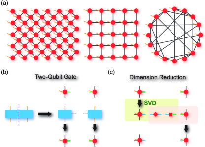
Figure 1: (a) Three examples of graph geometries: the Sycamore processor, a square lattice as well as an arbitrarily connected lattice from left to right. Each red circle stands for one qubit, and the black lines means the connections between the qubits, which also correspond to the auxiliary indexes of the tensor network states. The orange lines represent the physical indexes. (b) Two-qubit gate operation. The left rectangle with four orange lines and a dashed cut in between represents the splitting of a two-qubit gate into two three dimensional tensors as in Eq.(2). The block on the right hand side of the black arrow shows the procedure of the two-qubit gate operation, which corresponds to Eqs.(3, 4). We have used a thicker green line to explicitly indicate that the size of the auxiliary index increases after the two-qubit gate operation. (c) SVD compression of the resulting tensors from two-qubit gate operation corresponding to Eqs.(5, 6).

For a two-qubit gate denoted as $O_{\sigma_{k}\sigma_{l}}^{\sigma_{k}^{\prime}\sigma_{l}^{\prime}}$ acting on the $k$- and $l$-th qubits, we first split it into two three-dimensional tensors using singular value decomposition (SVD) as in Guo et al. (2019)

$$O_{\sigma_{k}\sigma_{l}}^{\sigma_{k}^{\prime}\sigma_{l}^{\prime}}=\sum_{s=1}^{\chi_{o}}P_{\sigma_{k}s}^{\sigma_{k}^{\prime}}Q_{\sigma_{l}s}^{\sigma_{l}^{\prime}},$$ (2)

where the size of the auxiliary index $s$ is equal to the number of non-zero singular values, denoted as $\chi_{o}=\dim(s)$. For a controlled gate $\chi_{o}=2$ while for the iSWAP gate as well as the fSim gate used in Ref. Arute et al. (2019) $\chi_{o}=4$. Assuming $A^{k}$ and $A^{l}$ are connected by two auxiliary indexes $a^{k}_{m}$ and $a^{l}_{n}$, then the two-qubit gate operation on $A^{k}$ and $A^{l}$ can be denoted as

$$A^{\sigma_{k}^{\prime}}_{[a_{1}^{k}\dots a^{k}_{\dim(\mathcal{E}_{k})}]_{m}\mathbf{a}_{m}^{k}}\leftarrow\sum_{\sigma_{k}}P_{\sigma_{k}s}^{\sigma_{k}^{\prime}}A^{\sigma_{k}}_{a_{1}^{k}\dots a^{k}_{\dim(\mathcal{E}_{k})}};$$ (3)

$$A^{\sigma_{l}^{\prime}}_{[a_{1}^{l}\dots a^{l}_{\dim(\mathcal{E}_{l})}]_{n}\mathbf{a}_{n}^{l}}\leftarrow\sum_{\sigma_{l}}Q_{\sigma_{l}s}^{\sigma_{l}^{\prime}}A^{\sigma_{l}}_{a_{1}\dots a_{\dim(\mathcal{E}_{l})}},$$ (4)

where $[a_{1}^{k}\dots a^{k}_{\dim(\mathcal{E}_{k})}]_{m}=a_{1}^{k}\dots a_{m-1}^{k}a_{m+1}^{k}\dots a^{k}_{\dim(\mathcal{E}_{k})}$ and similarly for $[a_{1}^{l}\dots a^{l}_{\dim(\mathcal{E}_{l})}]_{n}$. We have also used $\mathbf{a}_{m}^{k}=a_{m}^{k}s$ and $\mathbf{a}_{n}^{l}=a_{n}^{l}s$, from which we can see clearly that after a two-qubit gate operation, the size of the auxiliary dimensions $a_{m}^{k}$ and $a_{n}^{l}$ are increased by a factor of $\chi_{o}$. The procedure of a two-qubit gate operation is also shown in Fig. 1(b). Single-qubit gates are not considered since they can be absorbed into two-qubit gates using gate fusion.

Compression by SVD. As we have pointed out in the introduction, an important feature of TNS based algorithms is that the resulting tensors after each two-qubit gate operation will be compressed, which can be done as follows. First we perform SVD on one of the resulting tensors in Eqs.(3, 4), say $A^{\sigma_{k}^{\prime}}$, as

$$A^{\sigma_{k}^{\prime}}_{[a_{1}^{k}\dots]_{m}\mathbf{a}_{m}^{k}}=\sum_{s^{\prime}s^{\prime\prime}}U^{\sigma_{k}^{\prime}}_{[a_{1}^{k}\dots]_{m}s^{\prime}}S_{s^{\prime}s^{\prime\prime}}V_{s^{\prime\prime}\mathbf{a}_{m}^{k}},$$ (5)

where only the nonzero singular values of $S$ are kept. Then one absorbs the matrix $V_{s^{\prime}\mathbf{a}_{m}^{k}}^{\prime}=\sum_{s^{\prime\prime}}S_{s^{\prime}s^{\prime\prime}}V_{s^{\prime\prime}\mathbf{a}_{m}^{k}}$ into the other tensor $A^{\sigma_{l}^{\prime}}$ as

$$A^{\sigma_{l}^{\prime}}_{[a_{1}^{l}\dots]_{n}s^{\prime}}\leftarrow\sum_{\mathbf{a}_{m}^{k}}A^{\sigma_{l}^{\prime}}_{[a_{1}^{l}\dots]_{n}\mathbf{a}_{m}^{k}}V_{s^{\prime}\mathbf{a}_{m}^{k}}^{\prime}.$$ (6)

Thus the size of the auxiliary index $a_{m}^{k}$ changes from $\dim(a_{m}^{k})\chi_{o}$ to $\dim(s^{\prime})$, satisfying $\dim(s^{\prime})\leq\dim(a_{m}^{k})\chi_{o}$, and similarly for $a_{n}^{l}$. The SVD compression procedure is shown in Fig. 1(c).

In the follow we identify two situations that we could have $\dim(s^{\prime})<\dim(a_{m}^{k})\chi_{o}$. First, when the $k$-th qubit is applied on by a two-qubit gate $O_{\sigma_{k}\sigma_{l}}^{\sigma_{k}^{\prime}\sigma_{l}^{\prime}}$ with $\chi_{o}=4$ for the first time, we will have from Eq.(5) that

$$\dim(s^{\prime})\leq\min(2\dim([a_{1}^{k}\dots]_{m}),\dim(\mathbf{a}_{m}^{k}))=2.$$ (7)

Namely the size of the corresponding auxiliary index can at most increase to $2$. We note that it is pointed out in Ref. Arute et al. (2019) that the fSim gate in the first two layers can be simplified into a controlled phase gate with $\chi_{o}=2$, since it can be decomposed into a controlled phase gate and an iSWAP gate. In contrast for our method the compression in Eq.(7) naturally results from Eqs.(5, 6) for any two-qubit gate satisfying $\chi_{o}>2$. Till now such compressions are only possible in the first few layers of gate operations. Now recalling that for the task of computing amplitudes, the quantum circuit starts from a separable quantum state corresponding to a bitstring $00\dots 0$ and is finally projected onto another separable quantum state corresponding to a bitstring $s_{1}s_{2}\dots s_{N}$ with $s_{n}=0,1$. To make use of the compression in Eq.(7) also in the last layers of gate operations, we can divide the two-body gates into two groups and perform a two-sided circuit evolution, that is, the first group of gates are applied onto the initial quantum state $|0\rangle^{N}$, while the second group of gates are applied inversely onto target quantum state $|s_{1}s_{2}\dots s_{N}\rangle$, then one obtains one amplitude by computing the overlap between two resulting TNS. This procedure is shown in Fig. 2(a).

In the second case, we consider the DCD pattern as described in Ref. Arute et al. (2019), which means that there are three successive two-qubit gates acting on the qubit pairs $(k,l)$, $(l,r)$ and $(k,l)$. We look at the tensor $A^{k}$ and assume that its auxiliary index $a^{k}_{m}$ is connected to the tensor $A^{l}$. $A^{k}$ is applied on twice, therefore the size of $a^{k}_{m}$ would increase to $\dim(a_{m}^{k})\chi_{o}^{2}$, while the sizes of the rest auxiliary indexes of $A^{k}$ remain unchanged. Moreover, DCD pattern often happens at the boundary, such that $A^{k}$ only has very few auxiliary indexes. As a result it is very likely that $\dim(a_{m}^{k})\chi_{o}^{2}>2\dim([a_{1}^{k}\dots a^{k}_{\dim(\mathcal{E}_{k})}]_{m})$, in which case the size of $a_{m}^{k}$ will get compressed by Eq.(5) and thus grows slower than by a factor of $\chi_{o}^{2}$. The occurrence of this pattern as well as the compression of the resulting tensors are shown in Fig. 2(b). We note that this compression is done automatically by Eqs.(5, 6) without additional manual efforts.

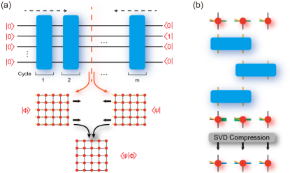
Figure 2: (a) Two-sided circuit evolution. Each blue rectangle represents a group of two-qubit gates (one cycle). The $m$ cycles are further divided into two groups as indicated by the vertical red dashed line in the middle of the circuit. The left cycles are applied onto the initial state $|0\rangle^{N}$ from left to right, while the right cycles are applied inversely onto the target state $|01\dots\rangle$ from right to left. The evolution results in two tensor network states as shown with the two lattices below the circuit. The physical indexes of those two tensor network states are then contracted, which results in the tensor network on the bottom with no open legs. (b) Automatic compression of the result tensors from the DCD pattern by SVD. Here each blue rectangle stands for a two-qubit gate.

Overlap between two tensor network states. As shown in Fig. 2(a), the two-sided circuit evolution will result in two TNS corresponding to two output quantum states $|\phi\rangle$ and $\langle\psi|$ respectively. Writing $|\phi\rangle=\mathcal{F}(A^{\sigma_{1}}_{a_{1}^{1}\dots a^{1}_{\dim(\mathcal{E}_{1})}}\dots A^{\sigma_{N}}_{a_{1}^{N}\dots a^{N}_{\dim(\mathcal{E}_{N})}})$ and $\langle\psi|=\mathcal{F}(B^{\sigma_{1}}_{b_{1}^{1}\dots b^{1}_{\dim(\mathcal{E}_{1})}}\dots B^{\sigma_{N}}_{b_{1}^{N}\dots b^{N}_{\dim(\mathcal{E}_{N})}})$, the overlap of $|\phi\rangle$ and $\langle\psi|$ can be computed by contracting all the physical indexes between them, that is,

$$\langle\psi|\phi\rangle=\mathcal{F}(C_{c_{1}^{1}\dots c^{1}_{\dim(\mathcal{E}_{1})}}\dots C_{c_{1}^{N}\dots c^{N}_{\dim(\mathcal{E}_{N})}}),$$ (8)

where $C_{c_{1}^{l}\dots c^{l}_{\dim(\mathcal{E}_{j})}}=\sum_{\sigma_{l}}A^{\sigma_{l}}_{a_{1}^{l}\dots a^{l}_{\dim(\mathcal{E}_{l})}}B^{\sigma_{l}}_{b_{1}^{l}\dots b^{l}_{\dim(\mathcal{E}_{l})}}$ for $1\leq l\leq N$. Eq.(8) is a tensor network on graph $\mathcal{G}$. Directly contracting this tensor network will generally result in high-dimensional intermediate tensors which have to be stored distributedly, leading to cross-node data communication costs Guo et al. (2019). To overcome this difficulty, one can cut a few legs in Eq.(8) as done in Ref. Villalonga et al. (2019). For example, cutting the auxiliary dimension $c_{m}^{k}$ amounts to splitting the $m$-th leg of the tensor $C^{k}$ into $\dim(c_{m}^{k})$ slices (the same for the tensor which connects to $C^{k}$ via $c_{m}^{k}$), as a result the tensor network in Eq.(8) is split into $\dim(c_{m}^{k})$ sub tensor networks in which the auxiliary index $c_{m}^{k}$ is removed. Each sub tensor network produces a single scalar. Summing over these scalars results in the final amplitude.

In addition, we propose a heuristic algorithm to search for the optimal tensor contraction path. Based on the observation that current NISQ hardwares have a (quasi)-regular two-dimensional geometrical structure, we made three assumptions that an optimal tensor contraction path $\mathcal{P}_{i_{1}\dots i_{N}}$ needs to satisfy: 1) $\mathcal{P}_{i_{1}\dots i_{N}}$ starts from a qubit on the boundary; 2) the rank of the intermediate tensors appear along this path is bounded by a maximum value $\mathcal{M}$; 3) For each $m$, the subgraph formed by the qubits $\{i_{1},\dots,i_{m}\}$ is almost connected. These assumptions allow us to neglect most of the paths. And we are able to come up with an efficient searching algorithm using state compression dynamical programming technique, which is detailed in the supplementary sup .

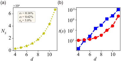
Figure 3: (a) Smallest number of required bitstrings $N_{s}$ as a function of circuit depth $d$ for gate fidelities shown in the text box. (b) Estimated run time $t$ as a function of depth $d$. The blue dashed line with square and the red dashed line with circle are results for the Sch$\ddot{\text{o}}$dinger-Feynman algorithm and our TNS based algorithm respectively.

Verification of RQCs. We demonstrate the efficiency of our algorithm by applying it to simulate RQCs running on a 53-qubit Sycamore processor, and then comparing its performance to the Sch$\ddot{\text{o}}$dinger-Feynman algorithm Markov et al. (2018). Our TNS based algorithm is a single-amplitude algorithm since the complexity of computing $M$ amplitudes is equal to $M$ times the complexity of computing a single amplitude. In contrast, the Sch$\ddot{\text{o}}$dinger-Feynman algorithm is a full-amplitude algorithm since computing a single amplitude is almost as hard as computing a bunch of $M$ amplitudes. Therefore for a fair comparison one needs to specify the smallest number of bitstrings $N_{s}$ required, for example, for the verification task. $N_{s}$ will in general increase as the fidelity $\mathcal{F}$ of the quantum circuit decreases, which can be computed as

$$\mathcal{F}=\prod\limits_{{\rm{g}}={G}}{(1-{e_{\rm{g}}})}\prod\limits_{{\rm{q}}=Q}{(1-{e_{\rm{q}}})}.$$ (9)

Here $G$ denotes the gate set, $e_{g}$ denotes the gate error rate, $Q$ denotes the qubit set and $e_{q}$ denotes readout error rate. The Sycamore processor used in Ref. Arute et al. (2019) has a single qubit error rate of $e_{1}=0.16\%$, two-qubit gate error rate of $e_{2}=0.62\%$, and readout error rate of $e_{q}=3.8\%$. To ensure that $\mathcal{F}$ is larger than $0$ with $3\sigma$, where $\sigma=1/\sqrt{N_{s}}$ denotes the statistical error, $N_{s}$ needs to satisfy $N_{s}\geq(3/F)^{2}$. We plot $N_{s}$ as a function of the circuit depth $d$ in Fig. 3(a).

In Fig. 3(b), we plot the estimated total run time $t$ for both algorithms as a function of $d$, where the blue dashed with square stands for the Sch$\ddot{\text{o}}$dinger-Feynman algorithm while the red dashed line with circle stands for our tensor network based algorithm. For the Sch$\ddot{\text{o}}$dinger-Feynman algorithm, we measure the time $t_{0}$ for a single path and then the total run time $t$ can be computed as $t=t_{0}N_{p}$ where $N_{p}$ is the total number of paths. For the TNS based algorithm, we compute the time $t_{s}$ for a single amplitude and then the total run time $t$ is simply $t=N_{s}t_{s}$. Both simulations are done using a single thread of the Intel-Xeon-Gold-6254 CPU ($3.1$ GHz). We note that our native implementation of the Sch$\ddot{\text{o}}$dinger-Feynman algorithm has a performance similar to the record in Ref. Arute et al. (2019), which is however still $1$ to $2$ orders of magnitudes slower than our TNS based algorithm for depths $6\leq d\leq 11$. Concretely, our TNS based algorithm is about $156$ times faster at $d=9$, and $19$ times faster at $d=11$. This would lead to significant cut down of the verification time. More details about the simulations down with both algorithms are in the supplementary sup .

We show the performance of our TNS based algorithm as the number of qubits $N$ increases in TABLE. 1. We can see that for relatively shallow circuits (especially when $d\leq 8$), our algorithm is much more preferable than the Sch$\ddot{\text{o}}$dinger-Feynman algorithm. For example for $d=6$, the run time with our algorithm increases very little as $N$ increases from $54$ to $72$, while for the Sch$\ddot{\text{o}}$dinger-Feynman algorithm it will be significantly more difficult (at least by a factor of $2^{9}$) since one has to store and manipulate two $36$-qubit sub circuits . Moreover, our algorithm can simulate the $104$-qubit RQC of Sycamore-like structure with up to $8$ depth, which is not possible for the Sch$\ddot{\text{o}}$dinger-Feynman algorithm simply due to the memory limitation (One has to store at least one $52$-qubit quantum state exactly).

Table 1: Run time to compute a single amplitude using TNS based algorithm. RQCs on Sycamore-like structures of sizes $54,60,66,72,104$ and depths from $6$ to $10$ are simulated using a single thread. The run time is shown in seconds. NA means that data is not available.

	6	7	8	9	10
Sycamore-54	24	19	143	1370	7260
Sycamore-60	24	30	337	4145	53007
Sycamore-66	29	82	1525	28968	267802
Sycamore-72	41	465	21669	278679	NA
Sycamore-104	107	15177	458576	NA	NA

In summary, we have presented a tensor network states based algorithm designed to simulate random quantum circuits with arbitrary geometry. We use singular value decomposition together with a two-sided circuit evolution algorithm to compress the size of the resulting tensor network from computing a single amplitude, which is further split into many smaller sub tensor networks using the cut technique. We then propose a heuristic algorithm to find the optimal tensor contraction path. We demonstrate with numerical simulations that our algorithm is of $1$ to $2$ orders of magnitudes faster than the Sch$\ddot{\text{o}}$dinger-Feynman algorithm when simulating random quantum circuits on the $53$-qubit Sycamore processor for depths $6\leq d\leq 11$, and show that for relatively shallow RQCs our algorithm has a much more preferable scaling than the Sch$\ddot{\text{o}}$dinger-Feynman algorithm as the number of qubits increases. Therefore we expect that our algorithm could be the method of choice for the fast verification of NISQ hardwares.