Self-motility of an active particle induced by correlations in the surrounding solution
Abstract
Current models of phoretic transport rely on molecular forces creating a “diffuse” particle–fluid interface. We investigate theoretically an alternative mechanism, in which a diffuse interface emerges solely due to a non-vanishing correlation length of the surrounding solution. This mechanism can drive self-motility of a chemically active particle. Numerical estimates indicate that the velocity can reach micrometers per second. The predicted phenomenology includes a bilinear dependence of the velocity on the activity and a possible double velocity reversal upon varying the correlation length.
Out-of-equilibrium behavior has been a research field of sustained interest, relevant to understanding the emergence of complexity de Groot and Mazur (1984); Sagués et al. (2007); Branscomb et al. (2017); Walker (2017). The last decade witnessed a rapidly growing engagement with self-phoretic, chemically active particles as a new paradigm thereof, which exhibits a wealth of phenomena, such as micro-phase separation Palacci et al. (2013), self-assembly of super-structures Aubret et al. (2018), and self-organized patterns of collective motion Lavergne et al. (2019); Singh et al. (2020). Additionally, phoresis has proven to be an effective, versatile transport mechanism at the microscale Marbach and Bocquet (2019); Battat et al. (2019); Tsuji et al. (2018), leading to a significant resurgence of interest also from a technological perspective.
Following the landmark review by Anderson Anderson (1989), the phenomenon of phoresis of particles suspended in a fluid is characterized by the presence of a driving thermodynamic field and by a transition region (also called “diffuse interface”) around the particle. The forces relevant for the phoretic displacement act within this region: its nonvanishing width gives rise to a response of the fluid medium even though the net sum of the forces and torques vanishes. Thus the particle is transported by the driving field while the system (particle plus fluid) is mechanically isolated, which sets this effect fundamentally apart from that of transport by an external force. The thermodynamic driving field usually comprises an externally imposed gradient in one of the state-parameters (such as composition, temperature, etc.) of the fluid, or of an electric field in the case of a charged particle in an electrolyte. The alternative case, in which the particle itself generates the driving field — a scenario also envisioned by Anderson Anderson (1989) — has recently received much attention under the generic name of “self-phoresis” Golestanian et al. (2005); Ruckner and Kapral (2007); Golestanian et al. (2007); Moran and Posner (2017). Experimentally, self-propelled particles have been realized most often in the form of so-called Janus particles. In a typical scenario, such particles are immersed in a multi-component fluid solution and promote catalytic reactions which vary across their surfaces, leading to self-electrophoresis Paxton et al. (2004); Fournier-Bidoz et al. (2005) or self-chemiophoresis Golestanian et al. (2005); Palacci et al. (2013); Brown and Poon (2014); Simmchen et al. (2016); Singh et al. (2017). Alternatively, the particles behave as heat sources, leading to self-thermophoresis through a single-component fluid Kroy et al. (2016) or self-chemiophoresis via demixing of a critical binary liquid mixture Volpe et al. (2011).
A common ingredient in the models, which have so far addressed phoretic Anderson (1989) and self-phoretic Golestanian et al. (2007); Würger (2015); Samin and van Roij (2015); Kroy et al. (2016); Moran and Posner (2017); Brown et al. (2017); Ibrahim et al. (2017) phenomena, is a direct physical interaction between the particle and the molecules of the surrounding fluid 111The paradigmatic setups one has considered involve either electrostatic forces or dispersion forces between the particle and the components of the fluid solution Moran and Posner (2017).. The corresponding non-vanishing interaction range provides the aforementioned diffuse interfacial region, where the internal forces and torques act and induce motion. Here, we propose an alternative transport mechanism which does not require this direct, extended interaction: instead, the interfacial region is diffuse because the fluid exhibits a non-vanishing correlation length. Although the phenomenology driven by this mechanism could also be called “phoresis” (in accordance with the definition proposed by Anderson Anderson (1989)), we coin the notion of “correlation–induced transport” in order to distinguish it from the usual one, which necessarily invokes a direct, spatially extended interaction.
Here we focus on the example of chemiophoresis, for which physically insightful analytical expressions can be derived, in order to illustrate the correlation–induced transport. However, the conceptual framework discussed below is expected to exhibit a very general applicability for other types of phoresis — albeit significantly more technically involved. For clarity and simplicity, we consider a rigid, spherical particle (radius ), immersed in a solution, i.e., a solvent plus a single solute species (called “the chemical” in the following). The particle is active, i.e., it is a source or sink of the chemical. The two main approximations are a spatially and temporally constant temperature and mass density of the solution, and a slow motion of the particle SM . Consequently, the state of the solution can be characterized de Groot and Mazur (1984) by the instantaneous stationary profiles of, e.g., the mass density of the chemical or, equivalently, of its number density valid for small Péclet numbers, and of the velocity field of the solution valid for small Reynolds and Mach numbers. Thus, is determined by the constraint of mass conservation for the chemical:
| (1) |
Here is the mobility of the chemical within the solution, while is the body force density acting on the chemical and which drives its diffusion. Likewise, follows from the balance between this body force and the fluid stresses, as expressed by the Stokes equation for incompressible flow,
| (2) |
in terms of the stress tensor ( is the viscosity of the solution, the pressure field enforcing incompressibility, and the identity tensor). Complementarily to the slow particle dynamics, one assumes local equilibrium for the chemical Anderson (1989), so that
| (3) |
in terms of its chemical potential . The latter is modelled by means of a free energy functional Anderson et al. (1998) (we take spherical coordinates with the origin at the center of the particle; denotes the volume element):
| (4) |
so that
| (5) |
Here, is a local free energy density, and is a potential energy (which has a non-zero and finite range) generated by the particle 222For an incompressible solution, is actually the difference in interaction of the particle with a molecule of solute and with a molecule of solvent, respectively de Groot and Mazur (1984).. In Eq. (4), the term accounts for the range of the molecular interactions between the dissolved molecules of the chemical 333More precisely, can be directly related to the second moment of the attractive part of the pair potential between the molecules of the chemical.. The relevant control parameters of this model for the chemical are and the temperature (implicit in the definition of ). However, it turns out (see, c.f., Eq. (Self-motility of an active particle induced by correlations in the surrounding solution)) that the results depend only on and the correlation length for a reference density 444The free energy in Eq. (4), with and linearized in , provides the equilibrium correlation function ., without the need to specify the dependence on temperature.
Finally, one has to specify boundary conditions: at infinity, a homogeneous equilibrium state is recovered, i.e., a vanishing velocity of the fluid solution and a constant chemical potential due to a reservoir (thereby also fixing the density at a value such that ):
| (6) |
On the surface of the particle, we impose a no-slip boundary condition in terms of the translational () and angular () velocities of the particle,
| (7) |
the boundary condition for the density, which follows from the surface term of the variation of the free energy functional 555In the limit , this boundary condition becomes actually irrelevant.,
| (8) |
and a prescribed current of the chemical, modelling the activity of the particle as a source of the chemical:
| (9) |
The positive constant represents the production rate of the chemical per area of the particle, and is the dimensionless activity, which can vary along the surface of the particle.
Equations (1–9), together with the condition that the particle does not experience any external force or torque, constitute a complete description for obtaining the velocities and of the particle for a prescribed activity function . If , the equilibrium state is a solution of the equations, which implies and . Thus, particle transport requires the non-equilibrium imbalance introduced by the chemical activity. We address two important aspects for solving this model. First, mechanical isolation of the whole system “particle + solution” holds because, according to Eq. (2), the medium transmitting forces from the particle to infinity is in local mechanical balance SM . Second, according to Eq. (2), the incompressibility constraint implies that the motion is driven by the spatially extended field , which (because of mechanical isolation) is the only source of flow vorticity 666The force can be decomposed into potential (i.e., irrotational) and solenoidal (i.e., divergence-free) components, . The potential component, , can be absorbed by the (auxiliary) hydrodynamic pressure field, , that enforces incompressibility; see also Eqs. (LABEL:eq:Omegacurlf, LABEL:eq:Vcurlf) in Ref. SM .. Combining Eqs. (3) and (5), one obtains
| (10) | |||||
Therefore, the transport, i.e., , requires either an explicit interaction between the particle and the chemical, i.e., , or a deviation of the solution from ideality, i.e., , which is associated with a non-vanishing correlation length in the solution. To the best of our knowledge, all previous studies of phoresis have analyzed and identified the case as the primary origin of particle transport. Here we address the opposite case (, ), for which the model [Eqs. (1–9)] implies that the spatially homogeneous equilibrium state (, ) would not be perturbed by the presence of a passive particle, i.e., . This case isolates the effect of correlations and already provides distinctive observable predictions.
A complete analytical solution for the correlation–induced transport velocity can be obtained if the deviations from homogeneity are small, i.e., for small values (weak activity) of the Damköhler number , where is the inverse thermal energy and is the diffusivity of the chemical: the dimensionless ratio quantifies the activity–induced “chemical crowding” near the particle against the opposing effect of diffusion. In this case, the spatial variation of and (via a possible dependence on the density ) can be neglected. Consequently, the “diffusion problem” for the density profile , posed by Eqs. (1, 3, 5, 6, 8, 9), is decoupled from the velocity field and can be solved first on its own. This can be carried out analytically, after linearizing in the small quantity . Subsequently, one solves the “hydrodynamical problem”, stated by Eqs. (2, 6, 7), with the body force in Eq. (3) determined by the profile obtained in the first step. Conveniently, the Lorentz reciprocal theorem allows one to sidestep the full solution of the “hydrodynamical problem” and to obtain expressions for and directly in terms of . Details of this procedure are collected in the Supplemental Material SM . By expanding the activity in terms of spherical harmonics,
| (11) |
one obtains a compact expression for the correlation–induced transport velocity:
| (12) |
with the velocity scale . In the Supplemental Material we provide 777See Eqs. (LABEL:eq:Gr–LABEL:eq:gp) in Ref. SM . the rather lengthy expressions for the purely geometrical factors , which depend only on the mathematical properties of the spherical harmonics, and for the dimensionless coefficients , which fully incorporate the dependence on the correlation length brought about by the physical model. The superscripts and denote the contributions by the radial and tangential components of the body force , respectively. The angular velocity turns out to vanish identically (see below).
Several general conclusions can be extracted already from this expression. Since Eq. (Self-motility of an active particle induced by correlations in the surrounding solution) is bilinear in the activity, the velocity is invariant under the transformation . This means that the direction of translation is insensitive to whether the particle acts as a source or a sink of the exchanged chemical. As shown by Eq. (10), a nonvanishing velocity requires a deviation from equilibrium (), as well as a deviation from homogeneity (). In the model of correlation–induced transport, both requirements are enforced by the activity, which explains the bilinear dependence. This is at variance with the case of standard phoresis, which gives rise to a velocity linear in the activity SM because usually suffices to bring about a relevant inhomogeneity. Another consequence of the symmetric form of the term in Eq. (10) is the absence of chirality, so that 888See the discussion of Eq. (LABEL:eq:tildeomega2) in Ref. SM .. In the standard model, on the contrary, the relative orientation of and will provide, in general, a preferred direction and sense of rotation, thus inducing a non-vanishing angular velocity.
The geometrical factors and can be expressed in terms of the Wigner 3j symbols SM , which induce “selection rules”: these factors will vanish unless and . Therefore, the sum in Eq. (Self-motility of an active particle induced by correlations in the surrounding solution) explicitly couples only pairs of “neighboring multipoles”. This result captures a major difference as compared to standard phoresis. For instance, an activity pattern lacking a dipole in Eq. (11) generically yields , while the same pattern of activity, together with a spherically symmetric potential , does not yield phoresis in the standard model 999See Ref. Golestanian et al. (2007). There is also the complementary case: a purely dipolar pattern (i.e., the simplest model of a Janus particle with no net production) renders SM , but in the standard model it yields a non-vanishing phoresis even for a spherically symmetric potential..
Another interesting feature of the transport velocity is revealed by considering the limit : the deviations from homogeneity are then localized within a thin layer (of thickness ) at the surface of the particle. In this case, the velocity can be expressed as an integral over the surface of the particle SM :
| (13) |
The integrand can be interpreted as a slip velocity for the “hydrodynamical problem” Anderson (1989), which is proportional to the tangential component of the density gradient,
| (14) |
with a local coefficient of phoretic mobility:
| (15) |
Due to the explicit dependence of on the activity (via ), the present mechanism of self-propulsion cannot be interpreted as “passive” transport in an external (albeit self-induced) gradient, which is another significant deviation from standard phoresis 101010Correlation–induced phoresis is also predicted for a passive particle in an external density gradient, yielding a transport velocity which is at least cubic in this gradient wip . This might explain why it has not received attention, being overshadowed by the mechanism based on an extended interaction.. Finally, we note that if because the tangential gradient vanishes SM . In the opposite limit , the velocity given by Eq. (Self-motility of an active particle induced by correlations in the surrounding solution) approaches a finite value 111111This conclusion is not trivial because the density field does require a finite in order to satisfy the boundary condition at infinity SM ., which depends only on and .
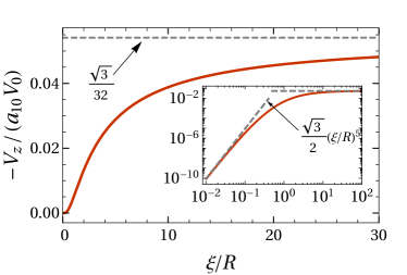
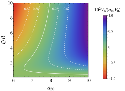
As an illustration SM , we study the simplest activity distribution with polar symmetry by retaining only monopolar and dipolar contributions: , , and in Eq. (11). For this case, Eq. (Self-motility of an active particle induced by correlations in the surrounding solution) renders , , with the function shown in Figure 1. The velocity depends linearly on the dipole strength and vanishes in the spherically symmetric limit . The asymptotic behaviors for or are given by the general results just discussed. If an additional quadrupolar activity contribution is included, Eq. (Self-motility of an active particle induced by correlations in the surrounding solution) gives , where and are monotonic functions of with opposite signs. Strikingly, this implies that the sign of can be altered by merely changing the correlation length (e.g., through temperature), while keeping the particle properties (i.e., the coefficients ) fixed. This rich behavior is illustrated in Fig. 2. For certain values of , such as , one indeed observes a reentrant regime where is negative at very small and very large , but positive in an intermediate range of correlation lengths.
These results allow one to estimate the magnitude of the velocity under realistic conditions. From Fig. 1, upon taking , one obtains in the regime . In order to estimate the velocity scale (see below Eq. (Self-motility of an active particle induced by correlations in the surrounding solution)), we approximate the local free energy of the chemical by the ideal gas expression , so that , and . With the typical values , , (viscosity of water), and (as for, e.g., the Pt catalyzed decomposition of hydrogen peroxide reported in Refs. Paxton et al. (2004); Brown et al. (2017)), one obtains at room temperature. For , the predicted velocity would be easily measurable; actually, the strong dependence on provides a broad range of variation covering the values reported from experiments for distinct types of systems Ebbens et al. (2012); Brown and Poon (2014); Simmchen et al. (2016); Singh et al. (2017); Das et al. (2020).
In summary, we have studied a mechanism of phoresis driven by correlations in the solution. Significant differences with respect to the standard mechanism of phoresis become evident: (i) The correlation–induced self-propulsion is bilinear in the activity, so that for the same activity pattern the two mechanisms predict distinct observable velocities. (ii) There is no self-rotation, regardless of the activity pattern. (iii) The correlation–induced phoresis cannot be understood as “passive” phoresis in an external (albeit self-induced) driving field. Already for simple activity patterns, the self-propulsion velocity exhibits remarkable features, including reentrant changes of sign obtained upon varying the correlation length (see Fig. 2). Numerical estimates for realistic conditions give values comparable to those observed experimentally, which are usually interpreted within the framework of the standard model of phoresis; correlation–induced phoresis provides an additional, plausible mechanism for addressing these observations.
Thus, our formalism opens the door to studying the role which correlations play in phoretic phenomena for a broad class of systems and geometries. In the physically relevant situation in which and , both correlation–induced transport and common phoresis would occur, including a coupling between correlations within the fluid and the inhomogeneities induced by . An extension of our analytical model could address their relative importance wip . In this regard, the present study constitutes, inter alia, an important addition to the theoretical machinery which is relevant for sorting and interpreting recent results pertaining to self-propulsion due to demixing in a binary liquid mixture (its order parameter playing the role of ). For example, this encompasses the numerical analysis in Ref. Samin and van Roij (2015), which incorporates nonlinear couplings (due to a non-vanishing Péclet number) in order to explain the emergence of self-motility, and the experimental observation of velocity reversals for certain self-propelled particles Gomez-Solano et al. (2017) following a change of illumination intensity (which changes the temperature distribution in the fluid and, correspondingly, the correlation length).
To conclude, we have identified and characterized a novel mechanism for self-phoresis of an active particle, which features potentially observable differences in comparison with the mechanism considered so far in the literature, and which can be controlled, e.g., via varying the temperature of the bath.
Acknowledgements.
A.D. acknowledges support by the Spanish Government through Grant FIS2017-87117-P (partially financed by FEDER funds).References
- de Groot and Mazur (1984) S. R. de Groot and P. Mazur, Non-Equilibrium Thermodynamics (Dover, New York, 1984).
- Sagués et al. (2007) F. Sagués, J. M. Sancho, and J. García-Ojalvo, “Spatiotemporal order out of noise,” Rev. Mod. Phys. 79, 829–882 (2007).
- Branscomb et al. (2017) E. Branscomb, T. Biancalani, N. Goldenfeld, and M. Russell, “Escapement mechanisms and the conversion of disequilibria; the engines of creation,” Phys. Rep. 677, 1–60 (2017).
- Walker (2017) S. I. Walker, “Origins of life: a problem for physics, a key issues review,” Rep. Prog. Phys. 80, 092601:1–40 (2017).
- Palacci et al. (2013) J. Palacci, S. Sacanna, A. P. Steinberg, D. J. Pine, and P. M. Chaikin, “Living crystals of light-activated colloidal surfers,” Science 339, 936 – 940 (2013).
- Aubret et al. (2018) A. Aubret, M. Youssef, S. Sacanna, and J. Palacci, “Targeted assembly and synchronization of self-spinning microgears,” Nature Phys. 14, 1114–1118 (2018).
- Lavergne et al. (2019) F. A. Lavergne, H. Wendehenne, T. Bäuerle, and C. Bechinger, “Group formation and cohesion of active particles with visual perception-dependent motility,” Science 364, 70–74 (2019).
- Singh et al. (2020) D. P. Singh, A. Domínguez, U. Choudhury, S. N. Kottapalli, M. N. Popescu, S. Dietrich, and P. Fischer, “Interface-mediated spontaneous symmetry breaking and mutual communication between drops containing chemically active particles,” Nat. Comm. 11, 2210:1–8 (2020).
- Marbach and Bocquet (2019) S. Marbach and L. Bocquet, “Osmosis, from molecular insights to large-scale applications,” Chem. Soc. Rev. 48, 3102 – 3144 (2019).
- Battat et al. (2019) S. Battat, J. T. Ault, S. Shin, S. Khodaparast, and H. A. Stone, “Particle entrainment in dead-end pores by diffusiophoresis,” Soft Matter 15, 3879 – 3885 (2019).
- Tsuji et al. (2018) T. Tsuji, Y. Sasai, and S. Kawano, “Thermophoretic manipulation of micro- and nanoparticle flow through a sudden contraction in a microchannel with near-infrared laser irradiation,” Phys. Rev. App. 10, 044005:1–18 (2018).
- Anderson (1989) J. L. Anderson, “Colloid transport by interfacial forces,” Annu. Rev. Fluid. Mech. 21, 61–99 (1989).
- Golestanian et al. (2005) R. Golestanian, T. B. Liverpool, and A Ajdari, “Propulsion of a molecular machine by asymmetric distribution of reaction products,” Phys. Rev. Lett. 94, 220801:1–4 (2005).
- Ruckner and Kapral (2007) G. Ruckner and R. Kapral, “Chemically powered nanodimers,” Phys. Rev. Lett. 98, 150603:1–4 (2007).
- Golestanian et al. (2007) R. Golestanian, T. B. Liverpool, and A Ajdari, “Designing phoretic micro- and nano-swimmers,” New J. Phys. 9, 126:1–9 (2007).
- Moran and Posner (2017) J. L. Moran and J. D. Posner, “Phoretic self-propulsion,” Annu. Rev. of Fluid Mech. 49, 511 – 540 (2017).
- Paxton et al. (2004) W. F. Paxton, K. C. Kistler, C. C. Olmeda, A. Sen, S. K. St. Angelo, Y. Y. Cao, T. E. Mallouk, P. E. Lammert, and V. H. Crespi, “Catalytic nanomotors: Autonomous movement of striped nanorods,” J. Am. Chem. Soc. 126, 13424–13431 (2004).
- Fournier-Bidoz et al. (2005) S. Fournier-Bidoz, A. C. Arsenault, I. Manners, and G. A. Ozin, “Synthetic self-propelled nanorotors,” Chem. Commun. , 441–443 (2005).
- Brown and Poon (2014) Aidan Brown and Wilson Poon, “Ionic effects in self-propelled pt-coated Janus swimmers,” Soft Matter 10, 4016 (2014).
- Simmchen et al. (2016) J. Simmchen, J. Katuri, W. E. Uspal, M. N. Popescu, M. Tasinkevych, and S. Sánchez, “Topographical pathways guide chemical microswimmers,” Nat. Comm. 7, 10598:1–9 (2016).
- Singh et al. (2017) Dhruv P Singh, Udit Choudhury, Peer Fischer, and Andrew G Mark, “Non-equilibrium assembly of light-activated colloidal mixtures,” Advanced Materials 29, 1701328 (2017).
- Kroy et al. (2016) K. Kroy, D. Chakraborty, and F. Cichos, “Hot microswimmers,” Eur. Phys. J. Spec. Topics 225, 2207 – 2225 (2016).
- Volpe et al. (2011) G. Volpe, I. Buttinoni, D. Vogt, H.-J. Kümmerer, and C. Bechinger, “Microswimmers in patterned environments,” Soft Matter 7, 8810–8815 (2011).
- Würger (2015) A. Würger, “Self-diffusiophoresis of Janus particles in near-critical mixtures,” Phys. Rev. Lett. 115, 188304:1–4 (2015).
- Samin and van Roij (2015) S. Samin and R. van Roij, “Self-propulsion mechanism of active Janus particles in near-critical binary mixtures,” Phys. Rev. Lett. 115, 188305:1–4 (2015).
- Brown et al. (2017) A. T. Brown, W. C. K. Poon, C. Holm, and J. de Graaf, “Ionic screening and dissociation are crucial for understanding chemical self-propulsion in polar solvents,” Soft Matter 13, 1200 – 1222 (2017).
- Ibrahim et al. (2017) Y. Ibrahim, R. Golestanian, and T. B. Liverpool, “Multiple phoretic mechanisms in the self-propulsion of a Pt-insulator Janus swimmer,” J. Fluid Mech. 828, 318 – 352 (2017).
- Note (1) The paradigmatic setups one has considered involve either electrostatic forces or dispersion forces between the particle and the components of the fluid solution Moran and Posner (2017).
- (29) For full details see the Supplemental Material at URL link, which also cites Refs. Happel and Brenner (1965); Abramowitz and Stegun (1972); Gradshteyn and Ryzhik (1994); Lorentz (1896); Kuiken (1996); Teubner (1982); Kim and Karrila (1991); Messiah (1999); Bender and Orszag (1978); Derjaguin et al. (1947).
- Anderson et al. (1998) D. M. Anderson, G. B. McFadden, and A. A. Wheeler, “Diffuse-interface methods in fluid mechanics,” Annu. Rev. Fluid Mech. 30, 139 – 165 (1998).
- Note (2) For an incompressible solution, is actually the difference in interaction of the particle with a molecule of solute and with a molecule of solvent, respectively de Groot and Mazur (1984).
- Note (3) More precisely, can be directly related to the second moment of the attractive part of the pair potential between the molecules of the chemical.
- Note (4) The free energy in Eq. (4), with and linearized in , provides the equilibrium correlation function .
- Note (5) In the limit , this boundary condition becomes actually irrelevant.
- Note (6) The force can be decomposed into potential (i.e., irrotational) and solenoidal (i.e., divergence-free) components, . The potential component, , can be absorbed by the (auxiliary) hydrodynamic pressure field, , that enforces incompressibility; see also Eqs. (LABEL:eq:Omegacurlf, LABEL:eq:Vcurlf) in Ref. SM .
- Note (7) See Eqs. (LABEL:eq:Gr–LABEL:eq:gp) in Ref. SM .
- Note (8) See the discussion of Eq. (LABEL:eq:tildeomega2) in Ref. SM .
- Note (9) See Ref. Golestanian et al. (2007). There is also the complementary case: a purely dipolar pattern (i.e., the simplest model of a Janus particle with no net production) renders SM , but in the standard model it yields a non-vanishing phoresis even for a spherically symmetric potential.
- Note (10) Correlation–induced phoresis is also predicted for a passive particle in an external density gradient, yielding a transport velocity which is at least cubic in this gradient wip . This might explain why it has not received attention, being overshadowed by the mechanism based on an extended interaction.
- Note (11) This conclusion is not trivial because the density field does require a finite in order to satisfy the boundary condition at infinity SM .
- Ebbens et al. (2012) Stephen Ebbens, Mei-Hsien Tu, Jonathan R Howse, and Ramin Golestanian, “Size dependence of the propulsion velocity for catalytic Janus-sphere swimmers,” Physical Review E 85, 020401(R) (2012).
- Das et al. (2020) Sayan Das, Zohreh Jalilvand, Mihail N Popescu, William E Uspal, Siegfried Dietrich, and Ilona Kretzschmar, “Floor- or ceiling-sliding for chemically active, gyrotactic, sedimenting Janus particles,” Langmuir 36, 7133–7147 (2020).
- (43) A. Domínguez et al, in preparation (2020).
- Gomez-Solano et al. (2017) J.R. Gomez-Solano, S. Samin, C. Lozano, P. Ruedas-Batuecas, R. van Roij, and C. Bechinger, “Tuning the motility and directionality of self-propelled colloids,” Sci. Rep. 7, 14891:1–12 (2017).
- Happel and Brenner (1965) J. Happel and H. Brenner, Low Reynolds Number Hydrodynamics (Prentice-Hall, Englewood Cliffs, NJ, 1965).
- Abramowitz and Stegun (1972) M. Abramowitz and I. R. Stegun, (Eds.) Handbook of mathematical functions (Dover, New York, 1972).
- Gradshteyn and Ryzhik (1994) I. S. Gradshteyn and I. M. Ryzhik, Table of Integrals, Series, and Products, 5th ed., edited by Alan Jeffrey (Academic Press, London, 1994).
- Lorentz (1896) H. A. Lorentz, “Eene algemeene stelling omtrent de beweging eener vloeistof met wrijving en eenige daaruit afgeleide gevolgen,” Zittingsverslag van de Koninklijke Akademie van Wetenschappen te Amsterdam 5, 168 – 175 (1896).
- Kuiken (1996) H. K. Kuiken, “H.A. Lorentz: A general theorem on the motion of a fluid with friction and a few results derived from it (translated from Dutch by H.K. Kuiken),” J. Eng. Math. 30, 19 –24 (1996).
- Teubner (1982) M. Teubner, “Motion of charged colloidal particles,” J. Chem. Phys. 76, 5564–5573 (1982).
- Kim and Karrila (1991) S. Kim and S. J. Karrila, Microhydrodynamics: Principles and Selected Applications (Butterworth–Heinemann, New York, 1991).
- Messiah (1999) Albert Messiah, Quantum Mechanics (Dover, New York, 1999).
- Bender and Orszag (1978) C. M. Bender and S. A. Orszag, Advanced Mathematical Methods for Scientists and Engineers (McGraw–Hill, 1978).
- Derjaguin et al. (1947) B. V. Derjaguin, G.P. Sidorenkov, E.A. Zubashchenkov, and E.V. Kiseleva, “Kinetic phenomena in boundary films of liquids,” Kolloidn. Zh. 9, 335–347 (1947).