Level attraction and exceptional points in a resonant spin-orbit torque system

Abstract

Level attraction can appear in driven systems where instead of repulsion two modes coalesce in a region separated by two exceptional points. This behavior was proposed for optomechanical and optomagnonic systems, and recently observed for dissipative cavity magnon-polaritons. We demonstrate that such a regime exists in a spin-orbit torque system where a magnetic oscillator is resonantly coupled to an electron reservoir. An instability mechanism necessary for mode attraction can be provided by applying an electric field. The field excites interband transitions between spin-orbit split bands leading to an instability of the magnetic oscillator. Two exceptional points then appear in the oscillator energy spectrum and the region of instability. We discuss conditions under which this can occur and estimate the electric field strength necessary for reaching the attraction region for a spin-orbit torque oscillator with Rashba coupling. A proposal for experimental detection is made using magnetic susceptibility measurements.

I Introduction

In noncentrosymmetric systems, the spin-orbit interaction provides mechanisms for spin angular momentum transfer and generation of spin-orbit torques [1]. Microscopically, this can be traced back to the spin Hall [2] and inverse spin galvanic effects [3, 4], where an electric field, can generate either a spin current or a spin polarization. In this paper we show how resonant spin-orbit torque devices can reveal aspects common to driven interacting systems such as mode attraction and exceptional points.

Spin-orbit torques play an important role in spintronics [5, 6, 7, 8, 9, 10, 11, 12, 13, 14, 15, 16, 17, 18, 19], with numerous applications including electric control and magnetization switching [20, 21, 22], coherent excitation and amplification of spin waves [23, 24, 25, 26], current-induced collective dynamics of topological spin textures [27, 28, 29, 30, 31], memory and logic devices [32, 33, 34], and neuromorphic computing [35]. Spin-orbit torque oscillators are of particular interest for many applications [36, 37, 38, 39, 40], including damping and antidamping torques [41] and other nontrivial features in high frequency response [42, 43].

Level attraction can occur at mode energy level crossings of an open system. It requires an instability of one of the modes, and in contrast to mode hybridization where two energy levels repel each other, energy levels coalesce for attraction, which in a certain way is reminiscent of mode synchronization [44]. The region of mode coalescence is bounded by two exceptional points where the eigenvectors become parallel in Hilbert space [45, 46]. These points are singularities and have been observed in microwave cavity applications. Their nontrivial topology may have utility in detecting devices [47, 48, 49].

Additionally, mode attraction has been studied in optomechanical circuits [44], cold atoms with negative mass instability [50], and coupled spin-photon systems [51, 52, 53, 54, 55, 56], and has been experimentally demonstrated for dissipative cavity magnon-polaritons [57, 58, 59, 60].

In this paper we show that a driven spin-orbit torque oscillator has a strong interaction regime where ferromagnetic resonance can be locked to interband electron transitions in a material with spin-orbit coupling. The exceptional points that appear can be electrically controlled. The nontrivial topological structure of the parameter space near the exceptional points [46] affects mode selection and is sensitive to damping and coupling strength.

The instability mechanism needed to reach the attractive regime is provided by spin accumulations created by an electric field applied to the electron system in a manner similar to inverse spin galvanic spin-orbit torques [5, 6]. We show that in a driven system spin accumulations modify an effective coupling between the resonances in magnetic and electron subsystems. As a result, the system near the energy level crossing can be described by a non-Hermitian Hamiltonian with a complex interaction constant.

Mode attraction can be experimentally detected by measuring magnetic susceptibility of a spin-orbit torque oscillator in the energy range where the ferromagnetic resonance of the magnetic oscillator is close to that of the electron band gap of the material with spin-orbit interaction. For a spin-orbit torque oscillator with Rashba coupling, we show that if the electric field is above some critical value, behavior of the susceptibility changes drastically in the region where magnetic and electron resonances strongly interact. Similar response has been reported for spin-orbit torque multi-layers in microwave waveguides [42]. We also demonstrate that it is possible to navigate around an exceptional point and explore its topological structure by sweeping strength and direction of the electric field. We estimate the critical field and discuss symmetry conditions required to realize this behavior in a Rashba system.

The paper is organized as follows. In Sec. II, we briefly review mode repulsion and attraction. A model for the spin-orbit torque oscillator is introduced in Sec. III. In Sec. IV, we discuss general properties of the magnetic susceptibility in an open spin-orbit torque system. These results are used in Sec. V to explain the level attraction regime, and are applied to the Rashba spin-orbit torque oscillator in Sec. VI, where we discuss possibilities for experimental detection. Concluding remarks are given in Section VII.

II Level attraction and exceptional points at a level crossing of an open system

We begin with a description of a physical picture at the mode energy level crossing of an open system. Suppose we have a mode described by the ladder operators $a$ and $a^{{\dagger}}$ and the frequency $\Omega$. Its interaction with another mode near the energy level crossing can be described by a linear Hamiltonian

$$H_{\ell}=\hbar\Omega a^{{\dagger}}a+\hbar\Delta c^{{\dagger}}c+\hbar g(c^{{\dagger}}a+a^{{\dagger}}c),$$ (1)

where $c$ and $c^{{\dagger}}$ are the ladder operators for the second mode, $\Delta$ is its frequency, and $g$ describes interaction between two modes. The spectrum of this interacting system is calculated as

$$\omega^{(\pm)}=\frac{\tilde{\Omega}+\tilde{\Delta}}{2}\pm\sqrt{\left(\frac{\tilde{\Omega}-\tilde{\Delta}}{2}\right)^{2}+g^{2}},$$ (2)

where we included phenomenological mode damping parameters $\Gamma$ and $\gamma$ into the complex frequencies $\tilde{\Omega}=\Omega-i\Gamma$ and $\tilde{\Delta}=\Delta-i\gamma$.

For an isolated system in thermodynamic equilibrium, $g$ is a real parameter, which ensures that $H_{\ell}$ is a Hermitian operator, so that Eq. (2) describes usual hybridization between two modes shown in Fig. 1 (a) with a gap proportional to $g^{2}$. As we show later on the example of a spin-orbit torque oscillator, level crossing of an open system can be also effectively described by Eq. (1). However, the interaction parameter $g$ in this case may become complex as result of interaction with an environment.

Let us consider a situation where $g$ is complex. While $\operatorname{Re}(g^{2})$ remains positive, the interation picture at the level crossing remains qualitatively the same as in Fig. 1 (a). This situation however changes drastically if $\operatorname{Re}(g^{2})$ becomes negative. It indicates an instability developing in the coupled system.

A detailed picture depends also on the imaginary part of $g^{2}$. If we can neglect $\operatorname{Im}(g^{2})$, in the region $|\Omega-\Delta|<4|g^{2}|$ the system enters a regime where $\omega^{(+)}$ and $\omega^{(-)}$ coalesce (see Fig. 1 b). Two exceptional points, where the Hamiltonian in Eq. (1) is not diagonalizable, mark the boundaries of this region. To realize this scenario, it is important to tune the dissipation channels so that $\Gamma\approx\gamma$ [44].

The imaginary part of $g^{2}$ modifies this behavior, and attraction may not be fully realized (see Fig. 1 c). Nevertheless, exceptional points still exist, and are determined from the equation $(\tilde{\Omega}-\tilde{\Delta})^{2}=-4g^{2}$, which is satisfied for

$$\frac{1}{2}(\Omega-\Delta)^{2} =|g^{2}|+|\operatorname{Re}(g^{2})|,$$ (3a)

$$\frac{1}{2}(\Gamma-\gamma)^{2} =|g^{2}|-|\operatorname{Re}(g^{2})|.$$ (3b)

The second equation here can be interpreted as a balance of energy dissipation in the system.

In the next sections, we show how this scenario can be realized for a spin-orbit torque oscillator driven by an electric field.

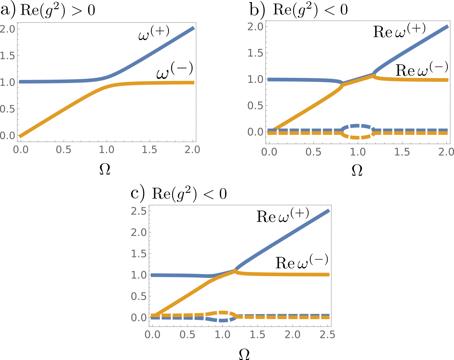
Figure 1: Level repulsion and attraction. (a) Typical hybridization picture between energy levels $\Delta=1$ and $\Omega$ in the case of $g^{2}>0$. (b) Level attraction picture with $\operatorname{Re}(g^{2})<0$ and $\operatorname{Im}(g^{2})=0$ when $\Gamma=\gamma$. The energy modes $\omega^{(\pm)}$ coalesce in the region $(\Omega-\Delta)<4g^{2}$ bounded by two exceptional points. (c) Mode attraction is broken when $\operatorname{Im}(g^{2})\neq 0$. One exceptional point, which satisfies Eqs. (3), is realized. Dashed lines show the imaginary parts of $\omega^{(\pm)}$.

III The model for a spin-orbit torque system

Resonant properties of a spin-orbit torque system can be described by a model [1, 5, 11] where conducting electrons in energy band $\varepsilon_{\bm{p}}$ interact with spin magnetic moment $\bm{S}$ via an $s$-$d$ exchange field $\Delta$ in the presence of a spin-orbit interaction $\bm{l}_{\bm{p}}$

$$H=\sum_{\bm{p}}\varepsilon_{\bm{p}}\psi^{{\dagger}}_{\bm{p}}\psi_{\bm{p}}+\sum_{\bm{p}}\bm{l}_{\bm{p}}\cdot\psi^{{\dagger}}_{\bm{p}}\bm{\sigma}\psi_{\bm{p}}-\Delta\bm{S}\cdot\sum_{\bm{p}}\psi^{{\dagger}}_{\bm{p}}\bm{\sigma}\psi_{\bm{p}},$$ (4)

where $\sigma_{i}$ ($i=x,y,z$) are the Pauli matrices, and $\psi_{\bm{p}}=(\psi_{\bm{p}\uparrow},\psi_{\bm{p}\downarrow})^{T}$, $\psi^{{\dagger}}_{\bm{p}}=(\psi^{{\dagger}}_{\bm{p}\uparrow},\psi^{{\dagger}}_{\bm{p}\downarrow})$, are the electron creation and annihilation operators with momentum $\bm{p}$ and spin $\sigma=(\uparrow,\downarrow)$.

We decompose $\bm{S}$ into a static part $\bm{S}_{0}$ and small dynamic perturbation $\delta\bm{S}$. By choosing $\bm{S}_{0}$ along the $z$ direction ($S_{0}=1$ hereafter), the static part of the Hamiltonian is written in the following form

$$H_{0}=\sum_{\bm{p}}\psi^{{\dagger}}_{\bm{p}}\begin{pmatrix}\varepsilon_{\bm{p}}-\Delta^{\prime}&l_{\bm{p}}^{(-)}\\ l_{\bm{p}}^{(+)}&\varepsilon_{\bm{p}}+\Delta^{\prime}\end{pmatrix}\psi_{\bm{p}},$$ (5)

where $\Delta^{\prime}=\Delta-l^{z}_{\bm{p}}$ and $l_{\bm{p}}^{(\pm)}=l_{\bm{p}}^{x}\pm il_{\bm{p}}^{y}$. The energy spectrum can be found by transforming to the basis where $H_{0}$ is diagonal, $\psi_{\bm{p}}=U_{\bm{p}}c_{\bm{p}}$, with the unitary transformation

$$U_{\bm{p}}=\begin{pmatrix}\dfrac{l_{\bm{p}}^{(-)}}{\Delta_{\bm{p}}}&-\dfrac{l_{\bm{p}}^{(-)}}{\Delta_{\bm{p}}}\\ \dfrac{\Delta_{\bm{p}}+\Delta^{\prime}}{\sqrt{N^{(+)}}}&\dfrac{\Delta_{\bm{p}}-\Delta^{\prime}}{\sqrt{N^{(-)}}}\end{pmatrix},$$ (6)

where $N^{(\pm)}=2\Delta_{\bm{p}}(\Delta_{\bm{p}}\pm\Delta^{\prime})$. The Hamiltonian in the new basis is

$$H_{0}=\sum_{\bm{p}}\left(\varepsilon_{\bm{p}}c^{{\dagger}}_{\bm{p}}c_{\bm{p}}+\Delta_{\bm{p}}c_{\bm{p}}^{{\dagger}}\sigma_{z}c_{\bm{p}}\right),$$ (7)

which has two energy bands split by the energy gap $\Delta_{\bm{p}}=\sqrt{l_{\bm{p}}^{2}-2l_{\bm{p}}^{z}\Delta+\Delta^{2}}$ due the exchange and spin-orbit couplings.

Interaction of the conduction band with the dynamic magnetization in Eq. (4) is given by

$$H_{i}=-\Delta\sum_{\bm{p}}\left(\delta S_{x}\psi^{{\dagger}}_{\bm{p}}\sigma_{x}\psi_{\bm{p}}+\delta S_{y}\psi^{{\dagger}}_{\bm{p}}\sigma_{y}\psi_{\bm{p}}\right).$$ (8)

We use a linearized Holstein-Primakoff representation [61] for the dynamic spin components, $\delta S_{x}=\sqrt{1/2}(a+a^{{\dagger}})$ and $\delta S_{y}=i\sqrt{1/2}(a-a^{{\dagger}})$, where $a$ and $a^{{\dagger}}$ satisfy boson commutation rules. After the unitary transformation in Eq. (6), the interaction part of the Hamiltonian becomes

$$H_{i}=\sum_{\bm{p}}\left(\bm{\lambda}_{\bm{p}}\cdot ac^{{\dagger}}_{\bm{p}}\bm{\sigma}c_{\bm{p}}+\bm{\lambda}_{\bm{p}}^{*}\cdot c^{{\dagger}}_{\bm{p}}\bm{\sigma}c_{\bm{p}}a^{{\dagger}}\right),$$ (9)

where the complex interaction parameter in the transformed frame is given by

$$\bm{\lambda_{p}}=\frac{\Delta}{\sqrt{2}}\frac{l_{\bm{p}}^{(-)}}{l_{\bm{p}}^{\perp}}\left(\frac{\Delta^{\prime}}{\Delta_{\bm{p}}},i,-\frac{l_{\bm{p}}^{\perp}}{\Delta_{\bm{p}}}\right),$$ (10)

where $\bm{l}_{\bm{p}}^{\perp}=(l^{x}_{\bm{p}},l^{y}_{\bm{p}},0)$ and $l_{\bm{p}}^{\perp}=|\bm{l}_{\bm{p}}^{\perp}|$.

Lastly, we include the Hamiltonian for the magnetization precessing with the the Kittel mode frequency $\Omega$ in a uniform magnetic field applied along the $z$ axis, $H_{m}=-\hbar\Omega S_{z}$. Using the representation $S_{z}=1-a^{{\dagger}}a$ [61], the complete Hamiltonian is written in the form of a two-band model interacting with an isolated bosonic mode

$$H=\hbar\Omega a^{{\dagger}}a+\sum_{\bm{p}}\left(\varepsilon_{\bm{p}}c^{{\dagger}}_{\bm{p}}c_{\bm{p}}+\Delta_{\bm{p}}c_{\bm{p}}^{{\dagger}}\sigma_{z}c_{p}\right)\\ +\sum_{\bm{p}}\left(ac_{\bm{p}}^{{\dagger}}(\bm{\lambda}_{\bm{p}}\cdot\bm{\sigma})c_{\bm{p}}+c^{{\dagger}}_{\bm{p}}(\bm{\lambda}_{\bm{p}}^{*}\cdot\bm{\sigma})c_{\bm{p}}a^{{\dagger}}\right),$$ (11)

where $c_{\bm{p}}=(c_{\bm{p}\uparrow},c_{\bm{p}\downarrow})^{T}$, $c^{{\dagger}}_{\bm{p}}=(c^{{\dagger}}_{\bm{p}\uparrow},c^{{\dagger}}_{\bm{p}\downarrow})$, describe destruction and creation of electrons in the upper ($\uparrow$) or lower ($\downarrow$) band. Notice that $\lambda^{z}_{\bm{p}}$ term commutes with $H_{0}$ and couples the boson mode to the difference in band occupation numbers.

IV Susceptibility for a driven spin-orbit torque oscillator

The nature of the dynamic regime of an interacting magnetic oscillator can be examined by looking at the magnetic susceptibility. Here, we derive the susceptibility $\chi(\omega)$ for the oscillator in Eq. (11) in the presence of spin-orbit torques produced by the conduction electrons that are driven externally by applying the field.

The susceptibility $\chi(\omega)$ is defined as the Fourier transform of a retarded Green’s function [62]

$$\chi(\omega)=-i\int_{0}^{\infty}dte^{i\omega t-\epsilon t}\langle[S^{(-)}(t),S^{(+)}(0)]\rangle,$$ (12)

where the circular components of the spin operator are $S^{(\pm)}=S_{x}\pm iS_{y}$. Here $\langle\ldots\rangle$ denotes averaging with respect to the density matrix $\rho=\exp(-H/k_{B}T)/\operatorname{\mathrm{Tr}}\exp(-H/k_{B}T)$ of the system in equilibrium, and $\epsilon\to 0^{+}$.

In terms of the model in Eq. (11), this includes calculating the retarded Green’s function for the boson mode

$$\mathopen{\hbox{${\langle}$}\kern-1.94444pt\leavevmode\hbox{${\langle}$}}a(t),a^{{\dagger}}(t^{\prime})\mathclose{\hbox{${\rangle}$}\kern-1.94444pt\leavevmode\hbox{${\rangle}$}}=-i\theta(t-t^{\prime})\operatorname{\mathrm{Tr}}\left\{[a(t),a^{{\dagger}}(t^{\prime})]\rho\right\},$$ (13)

where the operators are in the Heisenberg picture $a(t)=\exp(iHt/\hbar)a\exp(-iHt/\hbar)$.

We can simplify the model to see clearly the physics essential to our discussion. We drop the momentum index in Eq. (11) and consider a two-level system interacting with a quantum oscillator

$$H=\Omega a^{{\dagger}}a+\frac{\Delta}{2}s^{z}+a(\bm{\lambda}\cdot\bm{s})+(\bm{\lambda}^{*}\bm{s})a^{{\dagger}},$$ (14)

where $\bm{\lambda}$ is a complex interaction parameter, and the electron spin-$\frac{1}{2}$ operators are $s^{\alpha}=c^{{\dagger}}\sigma_{\alpha}c$. We use $\hbar=1$ for convenience and restore it when necessary.

The equation of motion [62] for the bosonic Green’s function is

$$i\frac{\partial}{\partial t}\mathopen{\hbox{${\langle}$}\kern-1.94444pt\leavevmode\hbox{${\langle}$}}a(t),a^{{\dagger}}(t^{\prime})\mathclose{\hbox{${\rangle}$}\kern-1.94444pt\leavevmode\hbox{${\rangle}$}}=\delta(t-t^{\prime})+\Omega\mathopen{\hbox{${\langle}$}\kern-1.94444pt\leavevmode\hbox{${\langle}$}}a(t),a^{{\dagger}}(t^{\prime})\mathclose{\hbox{${\rangle}$}\kern-1.94444pt\leavevmode\hbox{${\rangle}$}}\\ +\bm{\lambda}^{*}\cdot\mathopen{\hbox{${\langle}$}\kern-1.94444pt\leavevmode\hbox{${\langle}$}}\bm{s}(t),a^{{\dagger}}(t^{\prime})\mathclose{\hbox{${\rangle}$}\kern-1.94444pt\leavevmode\hbox{${\rangle}$}},$$ (15)

and is coupled with the equation of motion for the mixed Green’s function:

$$i\frac{\partial}{\partial t}\mathopen{\hbox{${\langle}$}\kern-1.94444pt\leavevmode\hbox{${\langle}$}}\bm{s}(t),a^{{\dagger}}(t^{\prime})\mathclose{\hbox{${\rangle}$}\kern-1.94444pt\leavevmode\hbox{${\rangle}$}}=i\Delta\mathopen{\hbox{${\langle}$}\kern-1.94444pt\leavevmode\hbox{${\langle}$}}\left[\hat{\bm{z}}\times\bm{s}(t)\right],a^{{\dagger}}(t^{\prime})\mathclose{\hbox{${\rangle}$}\kern-1.94444pt\leavevmode\hbox{${\rangle}$}}\\ +2i\mathopen{\hbox{${\langle}$}\kern-1.94444pt\leavevmode\hbox{${\langle}$}}a(t)[\bm{\lambda}\times\bm{s}(t)],a^{{\dagger}}(t^{\prime})\mathclose{\hbox{${\rangle}$}\kern-1.94444pt\leavevmode\hbox{${\rangle}$}}\\ +2i\mathopen{\hbox{${\langle}$}\kern-1.94444pt\leavevmode\hbox{${\langle}$}}\left[\bm{\lambda}^{*}\times\bm{s}(t)\right]a^{{\dagger}}(t),a^{{\dagger}}(t^{\prime})\mathclose{\hbox{${\rangle}$}\kern-1.94444pt\leavevmode\hbox{${\rangle}$}},$$ (16)

where $\hat{\bm{z}}$ is the unit vector along the $z$ axis.

Decoupling is achieved using the approximation, $\mathopen{\hbox{${\langle}$}\kern-1.94444pt\leavevmode\hbox{${\langle}$}}a(t)s^{\gamma}(t),a^{{\dagger}}(t^{\prime})\mathclose{\hbox{${\rangle}$}\kern-1.94444pt\leavevmode\hbox{${\rangle}$}}\approx\langle s^{\gamma}(t)\rangle\mathopen{\hbox{${\langle}$}\kern-1.94444pt\leavevmode\hbox{${\langle}$}}a(t),a^{{\dagger}}(t^{\prime})\mathclose{\hbox{${\rangle}$}\kern-1.94444pt\leavevmode\hbox{${\rangle}$}}$, which treats $\langle s^{\gamma}(t)\rangle$ as an external driving force. This assumption is reasonable if relaxation time of magnetic dynamics is much larger that the electron scattering time. Similar situation occurs for current generated spin transfer torques in magnetic textures [63].

Using the shorthand notation $G(t,t^{\prime})=\mathopen{\hbox{${\langle}$}\kern-1.94444pt\leavevmode\hbox{${\langle}$}}a(t),a^{{\dagger}}(t^{\prime})\mathclose{\hbox{${\rangle}$}\kern-1.94444pt\leavevmode\hbox{${\rangle}$}}$, $\tilde{G}(t,t^{\prime})=\mathopen{\hbox{${\langle}$}\kern-1.94444pt\leavevmode\hbox{${\langle}$}}a^{{\dagger}}(t),a^{{\dagger}}(t^{\prime})\mathclose{\hbox{${\rangle}$}\kern-1.94444pt\leavevmode\hbox{${\rangle}$}}$ and $\bm{F}(t,t^{\prime})=\mathopen{\hbox{${\langle}$}\kern-1.94444pt\leavevmode\hbox{${\langle}$}}\bm{s}(t),a^{{\dagger}}(t^{\prime})\mathclose{\hbox{${\rangle}$}\kern-1.94444pt\leavevmode\hbox{${\rangle}$}}$, we rewrite Eqs. (16) as

$$i\frac{\partial F_{x}}{\partial t} = -i\Delta F_{y}+\mathfrak{T}_{x}G+\mathfrak{T}^{*}_{x}\tilde{G},$$ (17a)

$$i\frac{\partial F_{y}}{\partial t} = i\Delta F_{x}+\mathfrak{T}_{y}G+\mathfrak{T}^{*}_{y}\tilde{G},$$ (17b)

$$i\frac{\partial F_{z}}{\partial t} = \mathfrak{T}_{z}G+\mathfrak{T}^{*}_{z}\tilde{G},$$ (17c)

where we introduce the torque, $\bm{\mathfrak{T}}=2i[\bm{\lambda}\times\langle\bm{s}(t)\rangle]$. This torque is exerted by the quantum oscillator on the electron system. This system of equations should be supplemented by the equation of motion for $\tilde{G}(t,t^{\prime})$. However, the contribution from $\tilde{G}(t,t^{\prime})$ can be neglected, since we are mostly interested in the region close to the resonance $\omega\approx\Omega$ (see Appendix A for details).

In what follows, we consider a stationary regime where the spin accumulations and, therefore, the torque $\mathfrak{T}$ are independent of time. In this situation, $G(t,t^{\prime})$ and $\bm{F}(t,t^{\prime})$ depend on $t-t^{\prime}$ and can be Fourier transformed according to $G(\omega)=\int_{-\infty}^{\infty}dt\exp(i\omega t)G(t)$. The equations of motion (16) and (17) in the frequency domain give

$$G(\omega)=\frac{1}{\omega-\Omega-\Sigma(\omega)}.$$ (18)

where

$$\Sigma(\omega)=\frac{1}{2}\frac{\lambda_{(+)}^{*}\mathfrak{T}_{(-)}}{\omega-\Delta}+\frac{1}{2}\frac{\lambda_{(-)}^{*}\mathfrak{T}_{(+)}}{\omega+\Delta}+\frac{\lambda_{z}^{*}\mathfrak{T}_{z}}{\omega},$$ (19)

with $\lambda_{(\pm)}=\lambda_{x}\pm i\lambda_{y}$ and $\mathfrak{T}_{(\pm)}=\mathfrak{T}_{x}\pm i\mathfrak{T}_{y}$.

The self-energy in Eq. (19) has two different contributions. The first contribution exists for thermodynamic equilibrium where $\langle s^{x}\rangle=\langle s^{y}\rangle=0$. Equilibrium is given by

$$\Sigma_{\mathrm{eq}}(\omega)=\frac{2\langle s^{z}\rangle}{\omega^{2}-\Delta^{2}}\left[i\omega(\bm{\lambda}^{*}\times\bm{\lambda})_{z}-\Delta(|\lambda_{x}|^{2}+|\lambda_{y}|^{2})\right],$$ (20)

where $\langle s^{z}\rangle=f_{\uparrow}-f_{\downarrow}$ with $f_{\sigma}$ being the population of the $\sigma=(\uparrow,\downarrow)$ energy level.

Close to the resonance $\omega\approx\Delta$, we can approximate $\omega+\Delta\approx 2\Delta$, and Eq. (20) can be written in a simplified form

$$\Sigma_{\mathrm{eq}}(\omega)=\frac{K_{\mathrm{eq}}}{\omega-\Delta},$$ (21)

where $K_{\mathrm{eq}}=\langle s^{z}\rangle\left[i(\lambda_{x}^{*}\lambda_{y}-\lambda_{y}^{*}\lambda_{x})-(|\lambda_{x}|^{2}+|\lambda_{y}|^{2})\right]$ is manifestly positive because in equilibrium $f_{\uparrow}<f_{\downarrow}$.

Out of thermodynamic equilibrium, a transverse spin accumulations $\langle s^{x}\rangle$ and $\langle s^{y}\rangle$ can appear. The self-energy then acquires an additional contribution $\Sigma(\omega)=\Sigma_{\mathrm{eq}}(\omega)+\delta\Sigma(\omega)$ from the torques $\mathfrak{T}_{(\pm)}$. In this decoupling scheme, $\delta\Sigma(\omega)$ is the second order term, which mixes $\lambda_{z}$ with interband spin transitions. In the region $\omega\approx\Delta$, this additional contribution can be approximated as

$$\delta\Sigma(\omega)=\frac{\lambda_{z}\lambda_{(+)}^{*}\langle\delta s^{(-)}\rangle}{\omega-\Delta},$$ (22)

where $\langle\delta s^{(-)}\rangle=\langle s^{x}\rangle-i\langle s^{y}\rangle$. We note that in contrast to $\delta\Sigma$, interband interactions $\lambda_{x}$ and $\lambda_{y}$ fully determine coupling to the oscillator mode in $\Sigma_{\mathrm{eq}}$.

According to Eqs. (21) and (22), the magnetic susceptibility that describes interaction between resonances in the electron and magnetic subsystems is written in the following form

$$\chi(\omega)=2\left[\omega-\Omega+i\Gamma-\frac{K}{\omega-\Delta+i\gamma}\right]^{-1},$$ (23)

where $K=K_{\mathrm{eq}}+\delta K$, and $\delta K$ is determined by Eq. (22). Here, we included $\Gamma$ and $\gamma$, which now have a meaning of phenomenological relaxation parameters for the magnetic and electron channels respectively.

Equations (21) and (22) show that in an open system the parameter $K$ that describes interaction between two resonances is generally complex as a result of external driving. Interaction of two modes near the energy level crossing in this situation can be described by a linear non-Hermitian Hamiltonian in Eq. (1) with a complex coupling $g=\sqrt{K}$.

V Mode attraction in a spin-orbit torque system driven by electric field

We apply our general results from Sec. IV to the model of the spin-orbit torque system in Eq. 11. Using Eqs. (21) and (22), and restoring the momentum index, we find the following expression for the self-energy of the magnetic oscillator

$$\Sigma(\omega)=-\frac{1}{2}\sum_{\bm{p}}\frac{\Delta^{2}}{\omega-2\Delta_{\bm{p}}}\left[\left(1+\frac{\Delta^{\prime}}{\Delta_{\bm{p}}}\right)^{2}\langle s^{z}_{\bm{p}}\rangle\right.\\ \left.+\frac{l_{\bm{p}}^{\perp}}{\Delta_{\bm{p}}}\left(1+\frac{\Delta^{\prime}}{\Delta_{\bm{p}}}\right)\langle\delta s^{(-)}_{\bm{p}}\rangle\right],$$ (24)

where $\langle\delta s^{\alpha}_{\bm{p}}\rangle=\langle c_{\bm{p}}^{{\dagger}}\sigma_{\alpha}c_{\bm{p}}\rangle$ for $\alpha=x,y$ can be interpreted as an average rate of interband electron transitions between $\varepsilon_{\bm{p}\sigma}=\varepsilon_{\bm{p}}\pm\Delta_{\bm{p}}$ bands, where upper (lower) sign is for $\sigma=\uparrow$ ($\sigma=\downarrow$), while $\langle s_{\bm{p}}^{z}\rangle=f_{\bm{p}\uparrow}-f_{\bm{p}\downarrow}$ denotes the difference in band occupation numbers with $f_{\bm{p}\sigma}=\{\exp\left[(\varepsilon_{\bm{p}\sigma}-\mu)/k_{B}T\right]+1\}^{-1}$ being the Fermi-Dirac distribution with the temperature $T$ and chemical potential $\mu$.

We note that the self-energy in Eq. (24) has a form of the self-energy of the Fano-Anderson model [64], $\Sigma(\omega)=\sum_{\bm{p}}g^{2}_{\bm{p}}/(\omega-2\Delta_{\bm{p}})$ with complex coupling $g_{\bm{p}}$. General analysis of this model is beyond the scope of this paper and will be studied elsewhere. For the rest of discussion, we use the strong exchange interaction approximation, $\Delta\gg l_{\bm{p}}$ [5]. In this regime, the energy splitting between two bands is independent of the momentum, $\Delta_{\bm{p}}\approx\Delta$, so that the susceptibility of the spin-orbit torque oscillator is given by Eq. (23) with

$$K=-2\Delta^{2}\sum_{\bm{p}}\left(\langle s^{z}_{\bm{p}}\rangle+\frac{l_{\bm{p}}}{2\Delta}\langle\delta s^{(-)}_{\bm{p}}\rangle\right).$$ (25)

In this equation, $\langle\delta s^{(-)}_{\bm{p}}\rangle=\langle\delta s^{x}_{\bm{p}}\rangle-i\langle\delta s^{y}_{\bm{p}}\rangle$ can be interpreted as the transverse electron spin accumulation in the local frame .

Spin accumulations can be induced, for example, via the inverse spin galvanic effect [3, 4]. Since spin-orbit interaction mixes spin and orbital degrees of freedom, a static electric field is able to induce spin accumulations in systems with broken inversion symmetry that, in turn, can exert a torque on a magneic oscillator [1].

We estimate these spin accumulations using a linear response approach in Appendix B. In the limit where the band splitting $\Delta$ is much greater than broadening due to impurity scattering, these spin accumulations are given by

$$\langle\delta s_{\bm{p}}^{x}\rangle = \frac{e(f_{\bm{p}\uparrow}-f_{\bm{p}\downarrow})}{2\Delta^{2}l_{\bm{p}}}\left[\bm{l}_{\bm{p}}\times\frac{\partial\bm{l}_{\bm{p}}}{\partial p_{\alpha}}\right]_{z}E_{\alpha},$$ (26a)

$$\langle\delta s_{\bm{p}}^{y}\rangle = \frac{e(f_{\bm{p}\uparrow}-f_{\bm{p}\downarrow})}{2\Delta^{2}l_{\bm{p}}}\left(\bm{l}_{\bm{p}}\cdot\frac{\partial\bm{l}_{\bm{p}}}{\partial p_{\alpha}}\right)E_{\alpha},$$ (26b)

where $\bm{E}$ is the electric field strength, and $e$ is the electron charge. In the transformed frame, these quantities play different roles: $\langle\delta s_{\bm{p}}^{y}\rangle$ contributes $\operatorname{Im}K$ and is involved mostly into the energy dissipation balance, see Eq. (3b), while $\langle\delta s_{\bm{p}}^{x}\rangle$ can be interpreted as a renormalization of the coupling constant between two resonances. Equations (26a) show that to create $\langle\delta s_{\bm{p}}^{x}\rangle$, the spin-orbit field $\bm{l}_{\bm{p}}$ should have at least two components.

Changing the sign of $\operatorname{Re}K$ drives the system toward instability. Since spin accumulations are proportional to $f_{\bm{p}\uparrow}-f_{\bm{p}\downarrow}$, the main contribution in Eq. (25) comes from the Fermi surface. To reach the instability regime, the following condition should be satisfied on the Fermi surface

$$1+\frac{eE_{\alpha}}{\Delta^{3}}\left[\bm{l}_{\bm{p}}\times\frac{\partial\bm{l}_{\bm{p}}}{\partial p_{\alpha}}\right]_{z}<0.$$ (27)

The $z$ component of the axial vector $\bm{l}_{\bm{p}}\times\partial(\bm{l}_{\bm{p}}/\partial p_{\alpha})E_{\alpha}$ in this expression can be interpreted as an effective field acting on the electron spin that competes with the exchange field $\Delta$ .

In order to reach the mode attraction regime, we need special symmetry conditions. First, since the second term in Eq. (27) is odd in $\bm{p}$, we need the original band to be noncentrosymmetric, $\varepsilon_{\bm{p}}\neq\varepsilon_{-\bm{p}}$, in order to preserve the contributions from Eqs. (26) after the summation over the Brillouin zone. Second, when $\langle\delta s_{\bm{p}}^{y}\rangle\ll\langle\delta s_{\bm{p}}^{x}\rangle$, level attraction can occur, as shown in Fig. 1 (b). We show how this can occur for a spin-orbit torque oscillator with Rashba coupling in the next section.

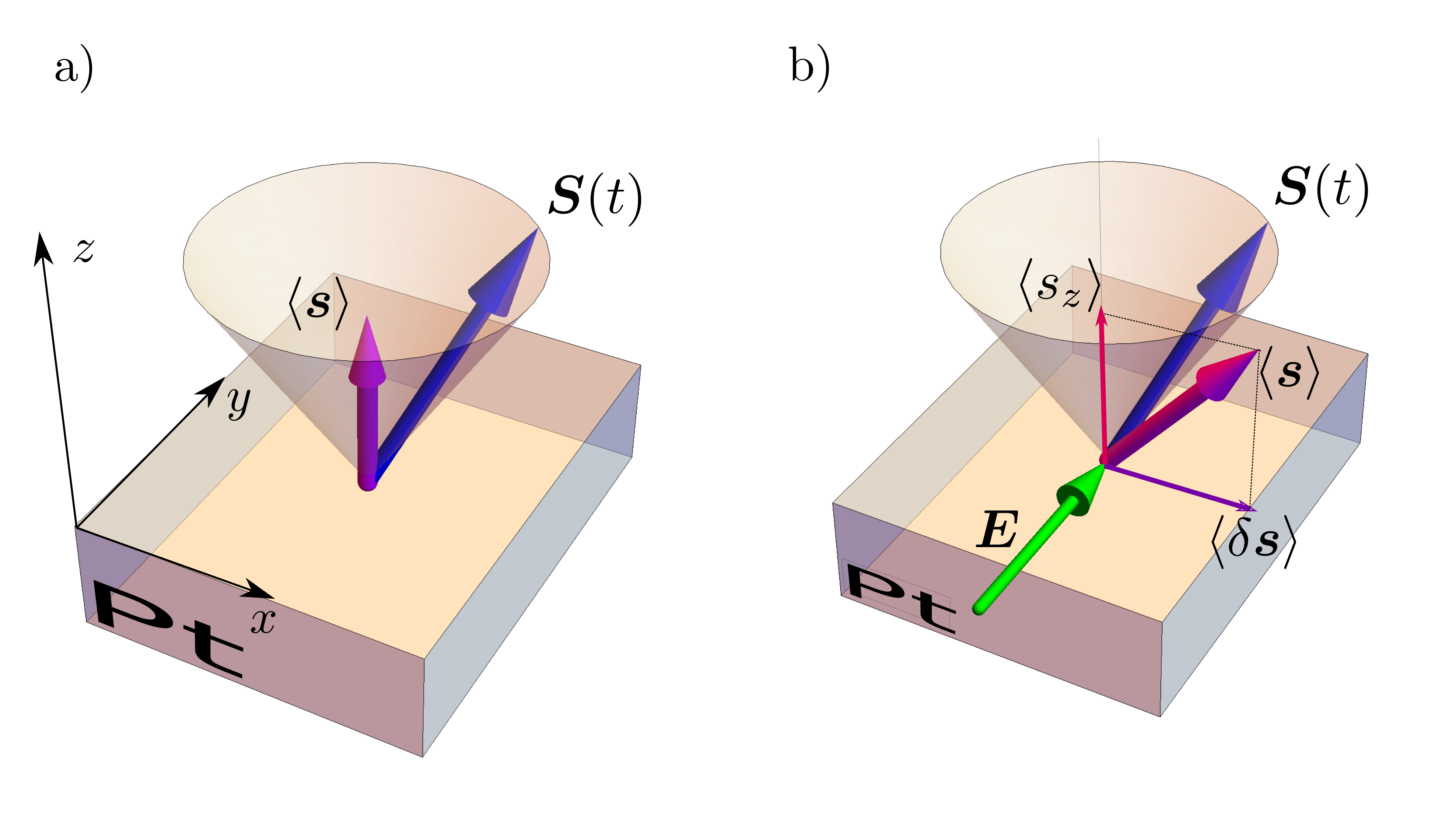
Figure 2: Schematic picture of a magnetic oscillator $\bm{S}(t)$ coupled to the material (Pt) with Rashba spin-orbit interaction $\frac{\alpha}{\hbar}(\bm{p}\times\hat{\bm{z}})\cdot\bm{\sigma}$ via $s$-$d$ exchange coupling. (a) In equilibrium, $\bm{S}(t)$ precesses around the quantization $z$ axis, which coincides with the direction of the magnetization of conduction electrons $\langle\bm{s}\rangle$. (b) Applying electric field $\bm{E}$ in noncentrosymmetric material creates a transverse spin accumulation $\langle\delta\bm{s}\rangle$ that modifies dynamics of the magnetic oscillator.

VI Realization for a spin-orbit torque oscillator with Rashba coupling

A physical system where our approach can be used is the spin-orbit torque oscillator with Rashba type of spin-orbit interaction. In two spatial dimensions, the Rashba model is described by the Hamiltonian in Eq. (4) with

$$\bm{l}_{\bm{p}}=\frac{\alpha}{\hbar}(\bm{p}\times\hat{\bm{z}}),$$ (28)

where $\bm{p}=(p_{x},p_{y},0)$ and $\alpha$ is the Rashba spin-orbit coupling [67]. Schematically, this setup is illustrated in Fig. 2. The spin accumulations in Eqs. (26) are reduced to

$$\langle\delta s_{\bm{p}}^{x}\rangle = \frac{e\alpha}{\hbar}\left(f_{\bm{p}\uparrow}-f_{\bm{p}\downarrow}\right)\frac{\bm{E}\cdot(\hat{\bm{z}}\times\bm{p})}{2p\Delta^{2}},$$ (29a)

$$\langle\delta s_{\bm{p}}^{y}\rangle = \frac{e\alpha}{\hbar}\left(f_{\bm{p}\uparrow}-f_{\bm{p}\downarrow}\right)\frac{(\bm{E}\cdot\bm{p})}{2p\Delta^{2}}.$$ (29b)

We note that for the Rashba model $\langle\delta s_{\bm{p}}^{x}\rangle$ is proportional to $\alpha(\bm{p}\times\bm{E})_{z}$, which may be interpreted as the $z$ component of the relativistic magnetic field in the coordinate frame of the moving electrons. Interestingly, when this field is strong enough to satisfy Eq. (27), system behavior becomes similar the two-oscillator model with negative-energy modes [44].

The electric field in Eqs. (29) couples to different components of the momentum. For example, if we apply the field along the $y$ axis, $\langle\delta s_{\bm{p}}^{y}\rangle$ becomes proportional to $p_{y}$, while $\langle\delta s_{\bm{p}}^{x}\rangle$ is determined by $p_{x}$. This can be used to manipulate relative contributions to real and imaginary parts of $K$ by rotating the system along the $z$ axis.

Suppose that we deal with a noncentrosymmetric band $\varepsilon_{\bm{p}}\neq\varepsilon_{-\bm{p}}$, in a situation where there is a mirror symmetry with respect to $p_{y}\to-p_{y}$. In this case, the contribution from $p_{y}$ vanishes, and the effective interaction between two resonance in Eq. (25) is estimated as follows

$$K=-\Delta^{3}\sum_{\bm{p}}\left(f_{\bm{p}\uparrow}-f_{\bm{p}\downarrow}\right)\left(1-\frac{e\alpha^{2}Ep_{x}\exp(i\beta)}{\hbar\Delta^{3}}\right),$$ (30)

where $\beta$ denote the angle between the electric field and $y$ axis. In a situation where $\Delta$ is much less than the Fermi energy $\varepsilon_{F}$, we can estimate $\operatorname{Re}K\approx g(\varepsilon_{F})S_{0}^{-1}(\Delta^{3}-e\xi\alpha^{2}p_{F}E\hbar^{-1})$, where $g(\varepsilon_{F})$ is the density of states at the Fermi level, $p_{F}$ denotes the Fermi momentum, and $\xi\lesssim 1$ and the dimensionless geometric factor that comes from the integration over the Fermi surface and reflect noncentrosymmetry of the band $\varepsilon_{\bm{p}}$. To reach the attractive regime, we need the electric field strength to be above the critical value, which makes $\operatorname{Re}K=0$ at the threshold. This field is estimated as

$$E_{c}=\frac{\Delta^{3}}{e\alpha^{2}k_{F}},$$ (31)

where $k_{F}$ is the Fermi momentum.

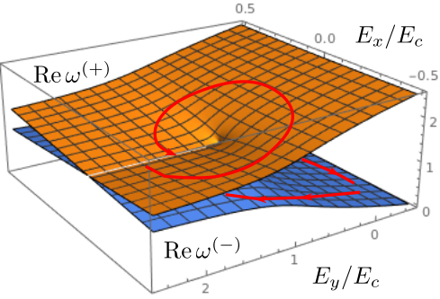
Figure 3: Real parts of $\omega^{(+)}$ and $\omega^{(-)}$ for the spin-orbit torque oscillator with the Rashba spin-orbit interaction on the $(E_{x},E_{y})$ plane. The branch cut, which is determined by Eq. (3b), terminates at the exceptional point given by Eq. (3a). A closed loop around the exceptional point is shown by the red line.

For the electric field applied along the $y$-direction ($\beta=0$), the contribution from $\langle s_{\bm{p}}^{y}\rangle$ vanishes, and $K$ is purely real. In contrast, applying the electric field along the mirror plane ($\beta=\pi/2$) will remove the contribution from $\langle\delta s_{\bm{p}}^{x}\rangle$. Therefore, by changing the direction of the electric field and its strength, we can in principle satisfy both Eqs. (3) and thus reach the exceptional point. We plot the real parts of $\omega^{(\pm)}$ on the $(E_{x},E_{y})$ plane in Fig. 3. This surface has a branch cut determined by Eq. (3b). By manipulating $E_{x}$ and $E_{y}$ it is possible to trace a closed loop around the exceptional point. For example, starting from the lower branch and then going through the branch cut, we would have $\omega^{(-)}\to\omega^{(+)}\to\omega^{(+)}\to\omega^{(-)}$ [45, 46], as shown in Fig. 3.

This opens a possible way for an electric-field switching of the oscillator regime. Suppose that at $E=0$ we have two hybridized modes with the frequencies $\omega^{(\pm)}\approx\Omega\pm\sqrt{(\delta/2)^{2}+K_{\mathrm{eq}}}$ where $\delta=\Omega-\Delta$ is the mode detuning parameter, and $K_{\mathrm{eq}}$ is a positive mode hybridization. Starting for example with the lower mode $\omega^{(-)}$ and slowly varying the electric field above $E_{c}$, we can go trough the branch cut (see Fig. 3), and after that decrease the electric field back to $E=0$. As a result, the systems will oscillate with the frequency $\omega^{(+)}$, which is normally separated from our initial mode $\omega^{(-)}$ by the energy gap of order $\sqrt{K_{\mathrm{eq}}}$.

For experimental observation, we need $\Delta$ withing the same range as the frequency of the ferromagnetic resonance $\Omega$. In typical spin-orbit torque materials [5], $\alpha\approx 10^{-12}$ eV/m, and $k_{F}\approx 10^{9}$ m^-1, so that $\alpha k_{F}/\Delta\lesssim 1$. This allows to estimate the minimal electric field strength as $\Delta k_{F}/e\approx 10^{4}$ V/cm.

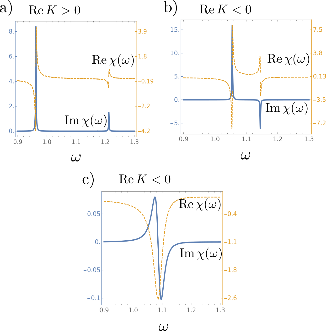
Figure 4: Magnetic susceptibility for the Rashba spin orbit torque oscillator (arbitrary units). Solid (dashed) line shows the imaginary (real) part of $\chi(\omega)$. (a) Two absorption peaks for $E<E_{c}$. (b) Resonance and anti-resonance in the case of $E>E_{c}$ and weak interaction $|\Omega-\Delta|\gtrsim|\operatorname{Re}K|$. (c) Strongly interacting case for $E>E_{c}$ and $|\Omega-\Delta|\lesssim|\operatorname{Re}K|$.

Experimentally, mode attraction can be identified by measuring susceptibility of the magnetic oscillator in the electric field. Below the critical field, one has usual behavior of $\operatorname{Im}\chi(\omega)$ showing two absorption peaks, as schematically demonstrated in Fig. 4 (a). In contrast, when $E>E_{c}$, the second resonance associated with electron transitions changes its sign, see Fig. 4 (b). The behavior of $\operatorname{Im}\chi(\omega)$ becomes particularly interesting in the region $|\Omega-\Delta|\lesssim|\operatorname{Re}K|$ where the two resonances strongly interact. In this situation, $\operatorname{Im}\chi(\omega)$ shows a sign change, while $\operatorname{Re}\chi(\omega)$ has a peak (Fig. 4 c). Interestingly, similar behavior of a response coefficient has been observed for a spin orbit torque system in a microwave waveguide [42].

VII Conclusions

Mode attraction can be observed in a Rashba spin-orbit torque system driven by an electric field. In noncentrosymmertic materials, the electric field couples to orbital motion of conduction electrons and thus creates an effective magnetic field, which renormalizes the interaction between electron and magnetic subsystems. In the case when the field strength is above the critical value $E_{c}$, the interaction between electron and magnetic resonances near the energy level crossing can be effectively described by a non-Hermitian Hamiltonian with a complex coupling constant. The real and imaginary parts of these constant can be separately controlled by different component of the electric field, when special symmetry conditions are met. This allows to realize an exceptional point in the energy spectrum of a driven dissipative spin-orbit torque system, and explore its topological structure by manipulating the electric field. This opens a way for electric-field selection and switching of a magnetic oscillator frequency.

Similar behavior may be expected in spin-transfer torque systems. However, detailed analysis of this topic is beyond the scope of this paper and requires a separate investigation.

Appendix A Equation of motion for $\tilde{G}(t,t^{\prime})$

Equations (15) and (17) should be supplemented by the equation of motion for $\tilde{G}(t,t^{\prime})$:

$$i\frac{\partial\tilde{G}}{\partial t}=-\Omega\tilde{G}-\bm{\lambda}\cdot\bm{F}.$$ (32)

Solving this equation together with Eqs (15) and (17) in the $\omega$-domain gives

$$\left[\omega-\Omega-\Sigma(\omega)\right]G(\omega)-A^{*}(\omega)\tilde{G}(\omega) = 1,$$ (33)

$$\left[\omega+\Omega+\Sigma^{*}(\omega)\right]\tilde{G}(\omega)+A(\omega)G(\omega) = 0,$$ (34)

where we also introduce

$$A(\omega)=\frac{1}{2}\frac{\lambda_{(+)}\mathfrak{T}_{(-)}}{\omega-\Delta}+\frac{1}{2}\frac{\lambda_{(-)}\mathfrak{T}_{(+)}}{\omega+\Delta}+\frac{\lambda_{z}\mathfrak{T}_{z}}{\omega}.$$ (35)

The solution for $G(\omega)$ is as follows

$$G(\omega)=\frac{\omega+\Omega+\Sigma^{*}(\omega)}{(\omega-\Omega-\Sigma(\omega))(\omega+\Omega+\Sigma^{*}(\omega))+|A(\omega)|^{2}},$$ (36)

which near $\omega\approx\Omega$ can be approximated by Eq. (18).

Appendix B Spin accumulations in the linear response regime

We outline calculation of the transverse spin accumulations $\langle\bm{s}^{\alpha}_{\bm{p}}\rangle$ ($\alpha=x,y$). For this purpose, we consider the linear response of the electron system with the Hamiltonian in Eq. (5) to the static electric field $\bm{E}$. In the frame where $H_{0}$ is diagonal, spin accumulations are given by the following Kubo formula [64]

$$\langle s_{\bm{p}}^{\alpha}\rangle=\int_{-\infty}^{0}dte^{st}\int_{0}^{\beta}d\tau\operatorname{\mathrm{Tr}}\left[\rho_{0}J^{\beta}(t-i\tau)s_{\bm{p}}^{\alpha}\right]E_{\beta},$$ (37)

where $\beta=(k_{B}T)^{-1}$, $s\to 0^{+}$, $\bm{J}$ is the electric current operator in the Heisenberg picture, and $\rho_{0}$ denotes density matrix for the noninteracting system.

For the Hamiltonian in Eq. (5), the current operator is given by the expression

$$J_{\alpha}=\sum_{\bm{p}}\frac{\partial\varepsilon_{\bm{p}}}{\partial p_{\alpha}}\psi^{{\dagger}}_{\bm{p}}\psi_{\bm{p}}+\sum_{\bm{p}}\frac{\partial\bm{l}_{\bm{p}}}{\partial p_{\alpha}}\cdot\psi^{{\dagger}}_{\bm{p}}\bm{\sigma}\psi_{\bm{p}},$$ (38)

which contains interband matrix elements proportional to the spin-orbit coupling. In the diagonal frame, the matrix elements of the current can be found using the following transformation rules for the Pauli matrices

$$U^{{\dagger}}\sigma_{x}U = -\frac{l_{\bm{p}}^{x}}{l_{\bm{p}}^{\perp}}\frac{\Delta^{\prime}}{\Delta_{\bm{p}}}\sigma_{x}-\frac{l_{\bm{p}}^{y}}{l_{\bm{p}}^{\perp}}\sigma_{y}+\frac{l_{\bm{p}}^{x}}{\Delta_{\bm{p}}}\sigma_{z},$$ (39)

$$U^{{\dagger}}\sigma_{y}U = -\frac{l_{\bm{p}}^{y}}{l_{\bm{p}}^{\perp}}\frac{\Delta^{\prime}}{\Delta_{\bm{p}}}\sigma_{x}+\frac{l_{\bm{p}}^{x}}{l_{\bm{p}}^{\perp}}\sigma_{y}+\frac{l_{\bm{p}}^{y}}{\Delta_{\bm{p}}}\sigma_{z},$$ (40)

$$U^{{\dagger}}\sigma_{z}U = -\frac{l_{\bm{p}}^{\perp}}{\Delta_{\bm{p}}}\sigma_{x}-\frac{\Delta^{\prime}}{\Delta_{\bm{p}}}\sigma_{z}.$$ (41)

In the transformed frame, only off-diagonal matrix elements of the current operator, $J_{\alpha}=\sum_{\bm{p}}c^{{\dagger}}_{\bm{p}\sigma}(\mathcal{J}^{\alpha}_{\bm{p}})_{\sigma\sigma^{\prime}}c_{\bm{p}\sigma^{\prime}}$, contribute to the transverse spin accumulations in Eq. (37). With the help of Eqs. (39)–(41), the off-diagonal matrix elements of the current are given by

$$\mathcal{J}_{\bm{p}}^{\alpha}=-\frac{\Delta^{\prime}}{\Delta_{\bm{p}}}\frac{1}{l^{\perp}_{\bm{p}}}\left(\bm{l}^{\perp}_{\bm{p}}\cdot\frac{\partial\bm{l}^{\perp}_{\bm{p}}}{\partial p_{\alpha}}\right)\sigma_{x}\\ +\frac{1}{l^{\perp}_{\bm{p}}}\left(\bm{l}^{\perp}_{\bm{p}}\times\frac{\partial\bm{l}^{\perp}_{\bm{p}}}{\partial p_{\alpha}}\right)_{z}\sigma_{y}-\frac{l^{\perp}_{\bm{p}}}{\Delta_{\bm{p}}}\frac{\partial l^{z}_{\bm{p}}}{\partial p_{\alpha}}\sigma_{x}.$$ (42)

After little algebra, we find the following expression for the spin accumulations from Eq. (37)

$$\langle s^{\alpha}_{\bm{p}}\rangle=iE_{\beta}\sum_{\sigma\sigma^{\prime}}\frac{f_{\bm{p}\sigma}-f_{\bm{p}\sigma^{\prime}}}{\varepsilon_{\bm{p}\sigma}-\varepsilon_{\bm{p}\sigma^{\prime}}}\frac{(\mathcal{J}^{\beta}_{\bm{p}})_{\sigma\sigma^{\prime}}(\sigma_{\alpha})_{\sigma^{\prime}\sigma}}{\varepsilon_{\bm{p}\sigma}-\varepsilon_{\bm{p}\sigma^{\prime}}-is}.$$ (43)

Taking $s\to 0$ limit, we find the following expressions for the transverse spin accumulations

$$\langle s_{\bm{p}}^{x}\rangle = -\frac{2(f_{\bm{p}\uparrow}-f_{\bm{p}\downarrow})}{(\varepsilon_{\bm{p}\uparrow}-\varepsilon_{\bm{p}\downarrow})^{2}}\operatorname{Im}(\mathcal{J}^{\alpha}_{\bm{p}})_{\uparrow\downarrow}E_{\alpha},$$ (44)

$$\langle s_{\bm{p}}^{y}\rangle = -\frac{2(f_{\bm{p}\uparrow}-f_{\bm{p}\downarrow})}{(\varepsilon_{\bm{p}\uparrow}-\varepsilon_{\bm{p}\downarrow})^{2}}\operatorname{Re}(\mathcal{J}^{\alpha}_{\bm{p}})_{\uparrow\downarrow}E_{\alpha},$$ (45)

which together with Eq. (42) gives Eqs. (26) in the limit $\Delta_{\bm{p}}\approx\Delta$ and $l^{z}_{\bm{p}}=0$.

References

- Manchon et al. [2019] A. Manchon, J. Železný, I. M. Miron, T. Jungwirth, J. Sinova, A. Thiaville, K. Garello, and P. Gambardella, Current-induced spin-orbit torques in ferromagnetic and antiferromagnetic systems, Rev. Mod. Phys. 91, 035004 (2019).
- Sinova et al. [2015] J. Sinova, S. O. Valenzuela, J. Wunderlich, C. H. Back, and T. Jungwirth, Spin Hall effects, Rev. Mod. Phys. 87, 1213 (2015).
- D’yakonov and Perel’ [1971] M. I. D’yakonov and V. I. Perel’, Possibility of orienting electron spins with current, Sov. Phys. JETP Lett. 13, 467 (1971).
- Edelstein [1990] V. M. Edelstein, Spin polarization of conduction electrons induced by electric current in two-dimensional asymmetric electron systems, Solid State Commun. 73, 233 (1990).
- Manchon and Zhang [2008] A. Manchon and S. Zhang, Theory of nonequilibrium intrinsic spin torque in a single nanomagnet, Phys. Rev. B 78, 212405 (2008).
- Chernyshov et al. [2009] A. Chernyshov, M. Overby, X. Liu, J. K. Furdyna, Y. Lyanda-Geller, and L. P. Rokhinson, Evidence for reversible control of magnetization in a ferromagnetic material by means of spin-orbit magnetic field, Nat. Phys. 5, 656 (2009).
- Manchon and Zhang [2009] A. Manchon and S. Zhang, Theory of spin torque due to spin-orbit coupling, Phys. Rev. B 79, 094422 (2009).
- Matos-Abiague and Rodríguez-Suárez [2009] A. Matos-Abiague and R. L. Rodríguez-Suárez, Spin-orbit coupling mediated spin torque in a single ferromagnetic layer, Phys. Rev. B 80, 094424 (2009).
- Miron et al. [2010] I. M. Miron, G. Gaudin, S. Auffret, B. Rodmacq, A. Schuhl, S. Pizzini, J. Vogel, and P. Gambardella, Current-driven spin torque induced by the rashba effect in a ferromagnetic metal layer, Nat. Mater. 9, 230 (2010).
- Gambardella and Miron [2011] P. Gambardella and I. M. Miron, Current-induced spin-orbit torques, Philos. Trans. Royal Soc. A 369, 3175 (2011).
- Wang and Manchon [2012] X. Wang and A. Manchon, Diffusive spin dynamics in ferromagnetic thin films with a rashba interaction, Phys. Rev. Lett. 108, 117201 (2012).
- Hals and Brataas [2013] K. M. D. Hals and A. Brataas, Phenomenology of current-induced spin-orbit torques, Phys. Rev. B 88, 085423 (2013).
- Hals and Brataas [2015] K. M. D. Hals and A. Brataas, Spin-motive forces and current-induced torques in ferromagnets, Phys. Rev. B 91, 214401 (2015).
- Freimuth et al. [2015] F. Freimuth, S. Blügel, and Y. Mokrousov, Direct and inverse spin-orbit torques, Phys. Rev. B 92, 064415 (2015).
- Sokolewicz et al. [2019] R. Sokolewicz, S. Ghosh, D. Yudin, A. Manchon, and M. Titov, Spin-orbit torques in a rashba honeycomb antiferromagnet, Phys. Rev. B 100, 214403 (2019).
- Haku et al. [2020] S. Haku, A. Ishikawa, A. Musha, H. Nakayama, T. Yamamoto, and K. Ando, Surface rashba-edelstein spin-orbit torque revealed by molecular self-assembly, Phys. Rev. Applied 13, 044069 (2020).
- Hibino et al. [2020] Y. Hibino, K. Yakushiji, A. Fukushima, H. Kubota, and S. Yuasa, Spin-orbit torque generated from perpendicularly magnetized Co/Ni multilayers, Phys. Rev. B 101, 174441 (2020).
- Filianina et al. [2020] M. Filianina, J.-P. Hanke, K. Lee, D.-S. Han, S. Jaiswal, A. Rajan, G. Jakob, Y. Mokrousov, and M. Kläui, Electric-field control of spin-orbit torques in perpendicularly magnetized films, Phys. Rev. Lett. 124, 217701 (2020).
- Saha et al. [2020] S. Saha, P. Flauger, C. Abert, A. Hrabec, Z. Luo, J. Zhou, V. Scagnoli, D. Suess, and L. J. Heyderman, Control of damping in perpendicularly magnetized thin films using spin-orbit torques, Phys. Rev. B 101, 224401 (2020).
- Liu et al. [2012] L. Liu, O. J. Lee, T. J. Gudmundsen, D. C. Ralph, and R. A. Buhrman, Current-induced switching of perpendicularly magnetized magnetic layers using spin torque from the spin Hall effect, Phys. Rev. Lett. 109, 096602 (2012).
- Wadley et al. [2016] P. Wadley, B. Howells, J. Železný, C. Andrews, V. Hills, R. P. Campion, V. Novák, K. Olejník, F. Maccherozzi, S. S. Dhesi, S. Y. Martin, T. Wagner, J. Wunderlich, F. Freimuth, Y. Mokrousov, J. Kuneš, J. S. Chauhan, M. J. Grzybowski, A. W. Rushforth, K. W. Edmonds, B. L. Gallagher, and T. Jungwirth, Electrical switching of an antiferromagnet, Science 351, 587 (2016).
- Shi et al. [2020] J. Shi, V. Lopez-Dominguez, F. Garesci, C. Wang, H. Almasi, M. Grayson, G. Finocchio, and P. K. Amiri, Electrical manipulation of the magnetic order in antiferromagnetic PtMn pillars, Nat. Electron. 3, 92 (2020).
- Gladii et al. [2016] O. Gladii, M. Collet, K. Garcia-Hernandez, C. Cheng, S. Xavier, P. Bortolotti, V. Cros, Y. Henry, J.-V. Kim, A. Anane, and M. Bailleul, Spin wave amplification using the spin Hall effect in permalloy/platinum bilayers, Appl. Phys. Lett. 108, 202407 (2016).
- Collet et al. [2016] M. Collet, X. De Milly, O. d. Kelly, V. V. Naletov, R. Bernard, P. Bortolotti, J. B. Youssef, V. Demidov, S. Demokritov, J. Prieto, et al., Generation of coherent spin-wave modes in yttrium iron garnet microdiscs by spin–orbit torque, Nat. Commun. 7, 1 (2016).
- Demidov et al. [2017] V. Demidov, S. Urazhdin, G. De Loubens, O. Klein, V. Cros, A. Anane, and S. Demokritov, Magnetization oscillations and waves driven by pure spin currents, Phys. Rep. 673, 1 (2017).
- Demidov et al. [2020] V. E. Demidov, S. Urazhdin, A. Anane, V. Cros, and S. O. Demokritov, Spin–orbit-torque magnonics, J. Appl. Phys. 127, 170901 (2020).
- Emori et al. [2013] S. Emori, U. Bauer, S.-M. Ahn, E. Martinez, and G. S. D. Beach, Current-driven dynamics of chiral ferromagnetic domain walls, Nat. Mater. 12, 611 (2013).
- Haazen et al. [2013] P. Haazen, E. Murè, J. Franken, R. Lavrijsen, H. Swagten, and B. Koopmans, Domain wall depinning governed by the spin Hall effect, Nat. Mater. 12, 299 (2013).
- Martin et al. [2020] F. Martin, K. Lee, A. Kronenberg, S. Jaiswal, R. M. Reeve, M. Filianina, S. Ji, M.-H. Jung, G. Jakob, and M. Kläui, Current induced chiral domain wall motion in CuIr/CoFeB/MgO thin films with strong higher order spin–orbit torques, Appl. Phys. Lett. 116, 132410 (2020).
- Sánchez-Tejerina et al. [2020] L. Sánchez-Tejerina, V. Puliafito, P. Khalili Amiri, M. Carpentieri, and G. Finocchio, Dynamics of domain-wall motion driven by spin-orbit torque in antiferromagnets, Phys. Rev. B 101, 014433 (2020).
- Hanke et al. [2020] J.-P. Hanke, F. Freimuth, B. Dupé, J. Sinova, M. Kläui, and Y. Mokrousov, Engineering the dynamics of topological spin textures by anisotropic spin-orbit torques, Phys. Rev. B 101, 014428 (2020).
- Bhowmik et al. [2014] D. Bhowmik, L. You, and S. Salahuddin, Spin hall effect clocking of nanomagnetic logic without a magnetic field, Nat. Nanotechnol. 9, 59 (2014).
- Olejník et al. [2017] K. Olejník, V. Schuler, X. Martí, V. Novák, Z. Kašpar, P. Wadley, R. P. Campion, K. W. Edmonds, B. L. Gallagher, J. Garcés, et al., Antiferromagnetic CuMnAs multi-level memory cell with microelectronic compatibility, Nat. Commun. 8, 1 (2017).
- Luo et al. [2020] Z. Luo, A. Hrabec, T. P. Dao, G. Sala, S. Finizio, J. Feng, S. Mayr, J. Raabe, P. Gambardella, and L. J. Heyderman, Current-driven magnetic domain-wall logic, Nature 579, 214 (2020).
- Torrejon et al. [2017] J. Torrejon, M. Riou, F. A. Araujo, S. Tsunegi, G. Khalsa, D. Querlioz, P. Bortolotti, V. Cros, K. Yakushiji, A. Fukushima, H. Kubota, S. Yuasa, M. D. Stiles, and J. Grollier, Neuromorphic computing with nanoscale spintronic oscillators, Nature 547, 428 (2017).
- Demidov et al. [2012] V. E. Demidov, S. Urazhdin, H. Ulrichs, V. Tiberkevich, A. Slavin, D. Baither, G. Schmitz, and S. O. Demokritov, Magnetic nano-oscillator driven by pure spin current, Nat. Mater. 11, 1028 (2012).
- Duan et al. [2014] Z. Duan, A. Smith, L. Yang, B. Youngblood, J. Lindner, V. E. Demidov, S. O. Demokritov, and I. N. Krivorotov, Nanowire spin torque oscillator driven by spin orbit torques, Nat. Commun. 5, 1 (2014).
- Cheng et al. [2016] R. Cheng, D. Xiao, and A. Brataas, Terahertz antiferromagnetic spin hall nano-oscillator, Phys. Rev. Lett. 116, 207603 (2016).
- Evelt et al. [2018] M. Evelt, C. Safranski, M. Aldosary, V. Demidov, I. Barsukov, A. Nosov, A. Rinkevich, K. Sobotkiewich, X. Li, J. Shi, et al., Spin Hall-induced auto-oscillations in ultrathin YIG grown on Pt, Sci. Rep. 8, 1269 (2018).
- Haidar et al. [2019] M. Haidar, A. A. Awad, M. Dvornik, R. Khymyn, A. Houshang, and J. Åkerman, A single layer spin-orbit torque nano-oscillator, Nat. Commun. 10, 1 (2019).
- Demidov et al. [2011] V. E. Demidov, S. Urazhdin, E. R. J. Edwards, and S. O. Demokritov, Wide-range control of ferromagnetic resonance by spin Hall effect, Appl. Phys. Lett. 99, 172501 (2011).
- Berger et al. [2018a] A. J. Berger, E. R. J. Edwards, H. T. Nembach, A. D. Karenowska, M. Weiler, and T. J. Silva, Inductive detection of fieldlike and dampinglike ac inverse spin-orbit torques in ferromagnet/normal-metal bilayers, Phys. Rev. B 97, 094407 (2018a).
- Berger et al. [2018b] A. J. Berger, E. R. J. Edwards, H. T. Nembach, O. Karis, M. Weiler, and T. J. Silva, Determination of the spin Hall effect and the spin diffusion length of Pt from self-consistent fitting of damping enhancement and inverse spin-orbit torque measurements, Phys. Rev. B 98, 024402 (2018b).
- Bernier et al. [2018] N. R. Bernier, L. D. Tóth, A. K. Feofanov, and T. J. Kippenberg, Level attraction in a microwave optomechanical circuit, Phys. Rev. A 98, 023841 (2018).
- Heiss [2004] W. D. Heiss, Exceptional points of non-Hermitian operators, J. Phys. A 37, 2455 (2004).
- Heiss [2012] W. D. Heiss, The physics of exceptional points, J. Phys. A 45, 444016 (2012).
- Chen et al. [2017] W. Chen, Ş. K. Özdemir, G. Zhao, J. Wiersig, and L. Yang, Exceptional points enhance sensing in an optical microcavity, Nature 548, 192 (2017).
- Hodaei et al. [2017] H. Hodaei, A. U. Hassan, S. Wittek, H. Garcia-Gracia, R. El-Ganainy, D. N. Christodoulides, and M. Khajavikhan, Enhanced sensitivity at higher-order exceptional points, Nature 548, 187 (2017).
- Zhong et al. [2019] Q. Zhong, J. Ren, M. Khajavikhan, D. N. Christodoulides, i. m. c. K. Özdemir, and R. El-Ganainy, Sensing with exceptional surfaces in order to combine sensitivity with robustness, Phys. Rev. Lett. 122, 153902 (2019).
- Kohler et al. [2018] J. Kohler, J. A. Gerber, E. Dowd, and D. M. Stamper-Kurn, Negative-mass instability of the spin and motion of an atomic gas driven by optical cavity backaction, Phys. Rev. Lett. 120, 013601 (2018).
- Grigoryan et al. [2018] V. L. Grigoryan, K. Shen, and K. Xia, Synchronized spin-photon coupling in a microwave cavity, Phys. Rev. B 98, 024406 (2018).
- Proskurin et al. [2019] I. Proskurin, R. Macêdo, and R. L. Stamps, Microscopic origin of level attraction for a coupled magnon-photon system in a microwave cavity, New J. Phys. 21, 095003 (2019).
- Yu et al. [2019] W. Yu, J. Wang, H. Y. Yuan, and J. Xiao, Prediction of attractive level crossing via a dissipative mode, Phys. Rev. Lett. 123, 227201 (2019).
- Grigoryan and Xia [2019] V. L. Grigoryan and K. Xia, Cavity-mediated dissipative spin-spin coupling, Phys. Rev. B 100, 014415 (2019).
- Karg et al. [2020] T. M. Karg, B. Gouraud, C. T. Ngai, G.-L. Schmid, K. Hammerer, and P. Treutlein, Light-mediated strong coupling between a mechanical oscillator and atomic spins 1 meter apart, Science 369, 174 (2020).
- Tserkovnyak [2020] Y. Tserkovnyak, Exceptional points in dissipatively coupled spin dynamics, Phys. Rev. Research 2, 013031 (2020).
- Harder et al. [2018] M. Harder, Y. Yang, B. M. Yao, C. H. Yu, J. W. Rao, Y. S. Gui, R. L. Stamps, and C.-M. Hu, Level attraction due to dissipative magnon-photon coupling, Phys. Rev. Lett. 121, 137203 (2018).
- Yang et al. [2019] Y. Yang, J. Rao, Y. Gui, B. Yao, W. Lu, and C.-M. Hu, Control of the magnon-photon level attraction in a planar cavity, Phys. Rev. Applied 11, 054023 (2019).
- Wang et al. [2019] Y.-P. Wang, J. W. Rao, Y. Yang, P.-C. Xu, Y. S. Gui, B. M. Yao, J. Q. You, and C.-M. Hu, Nonreciprocity and unidirectional invisibility in cavity magnonics, Phys. Rev. Lett. 123, 127202 (2019).
- Rao et al. [2019] J. W. Rao, C. H. Yu, Y. T. Zhao, Y. S. Gui, X. L. Fan, D. S. Xue, and C.-M. Hu, Level attraction and level repulsion of magnon coupled with a cavity anti-resonance, New J. Phys. 21, 065001 (2019).
- Holstein and Primakoff [1940] T. Holstein and H. Primakoff, Field dependence of the intrinsic domain magnetization of a ferromagnet, Phys. Rev. 58, 1098 (1940).
- Tiablikov [2013] S. Tiablikov, Methods in the Quantum Theory of Magnetism (Springer US, 2013).
- Kishine et al. [2010] J.-i. Kishine, A. S. Ovchinnikov, and I. V. Proskurin, Sliding conductivity of a magnetic kink crystal in a chiral helimagnet, Phys. Rev. B 82, 064407 (2010).
- Mahan [2013] G. D. Mahan, Many-particle physics (Springer Science & Business Media, 2013).
- Note [1] Neglecting terms of order means that and , where , see Eqs. (39)–(41). These equations show that and components of the electron spin in the laboratory frame are related to the spin accumulations in Eq. (24) by the rotation.
- Note [2] In other words, the electric-field-induced interband matrix elements of the electron current should be compared to the band gap .
- Bychkov and Rashba [1984] Y. A. Bychkov and E. I. Rashba, Oscillatory effects and the magnetic susceptibility of carriers in inversion layers, J. Phys. C 17, 6039 (1984).