The GALAH survey: effective temperature calibration from the InfraRed Flux Method in the Gaia system

Abstract

In order to accurately determine stellar properties, knowledge of the effective temperature of stars is vital. We implement Gaia and 2MASS photometry in the InfraRed Flux Method and apply it to over 360,000 stars across different evolutionary stages in the GALAH DR3 survey. We derive colour-effective temperature relations that take into account the effect of metallicity and surface gravity over the range $4000\,\rm{K}\lesssim T_{\rm{eff}}\lesssim 8000\,\rm{K}$, from very metal-poor stars to super solar metallicities. The internal uncertainty of these calibrations is of order 40$-$80 K depending on the colour combination used. Comparison against solar-twins, Gaia benchmark stars and the latest interferometric measurements validates the precision and accuracy of these calibrations from F to early M spectral types. We assess the impact of various sources of uncertainties, including the assumed extinction law, and provide guidelines to use our relations. Robust solar colours are also derived.

1 Introduction

The effective temperature ($T_{\rm{eff}}$) is one of the most fundamental stellar parameter, and it affects virtually every stellar property that we determine, be it from spectroscopy, or inferred by comparing against stellar models (e.g., Nissen & Gustafsson, 2018; Choi et al., 2018).

While angular diameters measured from interferometry provide the most direct way to measure effective temperatures of stars (provided bolometric fluxes can also be determined, see e.g., Code et al., 1976), they require a considerable investment of time. Such analysis require a careful assessment of systematic uncertainties, and they are biased towards bright targets, which are often saturated in modern photometric systems and all-sky surveys (e.g., White et al., 2013; Lachaume et al., 2019; Rains et al., 2020). Further, these stars are often the hardest to observe for large-scale spectroscopic surveys.

Among the many indirect methods to determine $T_{\rm{eff}}$ is the InfraRed Flux Method (hereafter IRFM), an almost model independent photometric technique originally devised to obtain angular diameters to a precision of a few per cent, and capable of competing against intensity interferometry in cases where a good flux calibration is achieved (Blackwell & Shallis, 1977; Blackwell et al., 1979, 1980). Over the years, the IRFM has been successfully applied to determine the effective temperatures of stars of different spectral types and metallicities (e.g., Blackwell & Shallis, 1977; Alonso et al., 1996b, 1999; Ramírez & Meléndez, 2005; González Hernández & Bonifacio, 2009; Casagrande et al., 2010).

The version of the IRFM used in this work has been previously validated against solar twins, HST absolute spectrophotometry and interferometric angular diameters (Casagrande et al., 2006, 2010). In particular, dedicated near-infrared photometry has been carried out to derive effective temperatures of interferometric targets with saturated 2MASS magnitudes (Casagrande et al., 2014). Our $T_{\rm{eff}}$ scale is widely used by many studies and surveys, and we now make it available into the Gaia photometric system. To do so, we implement Gaia photometry into the IRFM described in Casagrande et al. (2006, 2010). Also, thanks to Gaia parallaxes it is now possible to derive reliable surface gravities. We provide colour$-T_{\rm{eff}}$ relations which take into account the effect of metallicity and surface gravity by running the IRFM for all stars in the third Data Release (DR3) of the GALAH survey (Buder et al., 2021). This data release also includes stars observed with the same instrument setup, data reduction and analysis pipeline by the K2-HERMES (Wittenmyer et al., 2018; Sharma et al., 2019) and TESS-HERMES (Sharma et al., 2018) surveys.

We describe how Gaia photometry is implemented into our version of the IRFM in Section 2 and present colour$-T_{\rm{eff}}$ relations in Section 3. We benchmark our results against standard stars, assess the typical $T_{\rm{eff}}$ uncertainty of our calibrations and provide guidelines for their use in Section 4. Finally, we comment on the use of different colour indices and draw our conclusions in Section 5.

2 The InfraRed Flux Method using Gaia photometry

The IRFM can be viewed as the most extreme colour technique since it relies on the index defined by the ratio between the bolometric and the infrared monochromatic flux of a star. This ratio can be compared to that obtained using the same quantities defined on a stellar surface element, $\sigma T_{\rm{eff}}^{4}$ and $\mathcal{F}_{\mathrm{IR}}\rm{(model)}$, respectively (see e.g., Alonso et al., 1996a; Casagrande et al., 2006). If stellar and model fluxes are known, it is then possible to solve for $T_{\rm{eff}}$. As we describe later, this step is done iteratively in our version of the IRFM. The crucial advantage of the IRFM over other colour techniques is that, at least for spectral types hotter than early M-type, near-infrared photometry samples the Rayleigh–Jeans tail of stellar spectra, a region largely dominated by the continuum, with a roughly linear dependence on $T_{\rm{eff}}$. The model dependent term $\mathcal{F}_{\mathrm{IR}}\rm{(model)}$ is almost unaffected by metallicity, surface gravity and granulation, as extensively tested in the literature (e.g., Alonso et al., 1996b; Asplund & García Pérez, 2001; Ramírez & Meléndez, 2005; Casagrande et al., 2006; Casagrande, 2009; González Hernández & Bonifacio, 2009).

We use the implementation of the IRFM described in Casagrande et al. (2006, 2010), where for each star we now use Gaia $BP,RP$ and 2MASS $JHK_{s}$ photometry to derive the bolometric flux. The flux outside these bands (i.e., the bolometric correction) is estimated using a theoretical model flux at a given $T_{\rm{eff}},\log(g)$ and [Fe/H]. The infrared monochromatic flux is derived from 2MASS magnitudes only. An iterative procedure in $T_{\rm{eff}}$ is adopted to cope with the mildly model-dependent nature of the bolometric correction and surface infrared monochromatic flux. We interpolate over the Castelli & Kurucz (2003) grid of model fluxes, starting for each star with an initial estimate of its effective temperature and adopting the GALAH DR3 [Fe/H] and $\log(g)$, until convergence in $T_{\rm{eff}}$ is reached within 1K. The convergence is robust regardless of the initial $T_{\rm{eff}}$ estimate. The model dependence is expected to be small, and in Casagrande et al. (2006, 2010) we tested that using the MARCS grid of model fluxes (Gustafsson et al., 2008) affects the resulting $T_{\rm{eff}}$ only by few K for dwarfs and subgiants in the range $\simeq 4500-6500$ K.

For Gaia $BP$ and $RP$ magnitudes we use the Gaia-DR2 formalism described in Casagrande & VandenBerg (2018), which is based on the revised transmission curves and non-revised Vega zero-points provided by Evans et al. (2018). As described in Casagrande & VandenBerg (2018), this choice best mimics the photometric processing done by the Gaia team to reproduce phot_g_mean_mag, phot_bp_mean_mag and phot_rp_mean_mag given in Gaia DR2. In Appendix A we also implement Gaia EDR3 photometry, and provide calibrations for this system. We remark that although Gaia EDR3 is formally an independent photometric systems from Gaia DR2, differences are overall small for the sake of the $T_{\rm{eff}}$ derived from the IRFM (although the calibrations in the two systems should not be used interchangeably, as further discussed in Appendix A). We use $BP$ and $RP$ instead of $G$ magnitudes for a number of reasons: comparison with absolute spectrophotometry indicates that $BP$ and $RP$ are reliable and well standardized in the magnitude range $\simeq$ 5 to 16, which is relevant for our targets. On the contrary, $G$ magnitudes have a magnitude dependent offset, and are affected by uncalibrated CCD saturation for $G\lesssim 6$ (Evans et al., 2018; Casagrande & VandenBerg, 2018; Maíz Apellániz & Weiler, 2018). Further, the $BP$ and $RP$ bandpasses together have the same wavelength coverage as the $G$ bandpass.

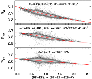
Figure 1: Gaia extinction coefficients as function of intrinsic stellar colours for our sample of stars (colour coded in gray by log-density). Red solid lines show the fits given in each panel. To estimate intrinsic colours needed for the fits, one can iterate starting from $(BP-RP)_{0}\simeq(BP-RP)-E(B-V)$. See Appendix B for a summary of the extinction coefficients for Gaia DR2, EDR3 and 2MASS under different extinction laws.

One of the most critical points when implementing the IRFM is the photometric absolute calibration (i.e., how magnitudes are converted into fluxes), which sets the zero-point of the $T_{\rm{eff}}$ scale. This is particularly important in the infrared, for which we use the same 2MASS prescriptions discussed in Casagrande et al. (2010). To verify that the zero-point of our $T_{\rm{eff}}$ scale is not altered by Gaia magnitudes, we derive $T_{\rm{eff}}$ for all stars in Casagrande et al. (2010) with a counterpart in Gaia (408 targets). Not unexpectedly, we find excellent agreement, with both mean and median $\Delta T_{\rm{eff}}=12\pm 2$ K ($\sigma=41$ K) and no trends as function of stellar parameters. This difference is robust, regardless of whether the stars used are those with the best Gaia quality flags. Although this difference is fully within the 20 K zero-point uncertainty of the reference $T_{\rm{eff}}$ scale of Casagrande et al. (2010), we correct for this small offset to adhere to the parent scale.

We apply the IRFM to over 620,000 spectra in GALAH DR3 for which [Fe/H], $\log(g)$, $BP,RP,J,H,K_{s}$ are available. About 40 percent of the targets have $E(B-V)$ from Green et al. (2019). For the remaining stars, we rescale reddening from Schlegel et al. (1998) with the same procedure described in Casagrande et al. (2019). Effective temperatures from the IRFM along with adopted values of reddening are available as part of GALAH DR3 (Buder et al., 2021, which also includes a comparison against the GALAH spectroscopic $T_{\rm{eff}}$.). To account for the spectral type dependence of extinction coefficients, in the IRFM we adopt the Cardelli et al. (1989)/O’Donnell (1994) extinction law, and for each star compute extinction coefficients with the synthetic spectrum at the $T_{\rm{eff}},\log(g)$ and [Fe/H] used at each iteration.

Figure 1 shows extinction coefficients for the Gaia filters as function of intrinsic (i.e., reddening corrected) stellar colour for our sample of stars. For the 2MASS system there is virtually no dependence on spectral type and the following constant values are found $R_{J}=0.899$, $R_{H}=0.567$ and $R_{Ks}=0.366$. These coefficients are in excellent agreement with those reported in Casagrande & VandenBerg (2014, 2018), obtained using the same extinction law. We discuss in Appendix B the effect of using different extinction laws on the derived colour$-T_{\rm{eff}}$ relations and extinction coefficients.

The use of constant extinction coefficients instead of colour dependent ones affects colour indices, and hence the effective temperatures derived from the relations of Section 3. This can be appreciated from the comparison in Figure 2, where the difference in colour obtained using constant or colour dependent extinction coefficients is amplified at high values of reddening for a given input $T_{\rm{eff}}$ . The fits of Figure 1 should thus be preferred to deredden colour indices involving Gaia bands, especially in regions of high extinction.

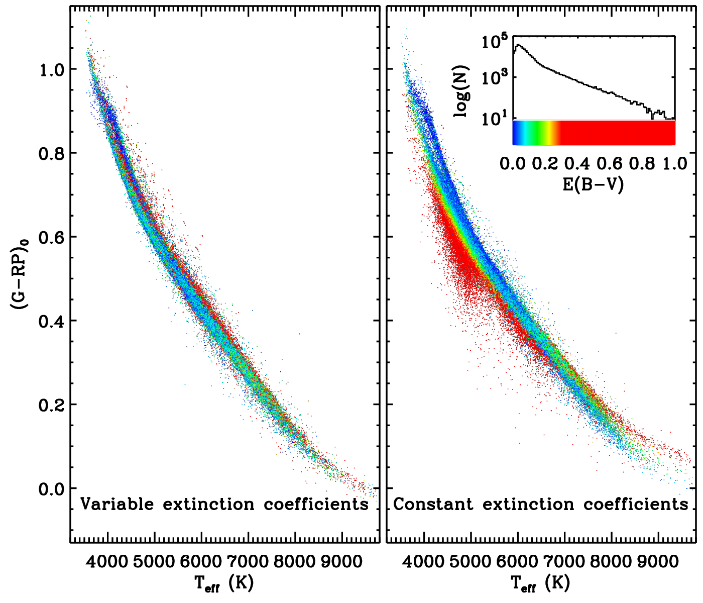
Figure 2: Left panel: colour-$T_{\rm{eff}}$ relation obtained from the IRFM in $(G-RP)_{0}$, where extinction coefficients are computed for each star individually. Right panel: colour-$T_{\rm{eff}}$ relation using the same input effective temperatures, but constant extinction coefficients to deredden the colour index. The importance of using variable extinction coefficients becomes visible for increasing values of reddening. Stars are colour coded by their $E(B-V)$ with the distribution shown in the inset.

3 Colour$-T_{\rm{eff}}$ relations

In order to derive colour-$T_{\rm{eff}}$ relations, we first apply a few quality cuts. We restrict ourselves to stars with the best GALAH DR3 spectroscopic parameters (flag_sp=0), and Gaia photometry $1.0+0.015\,(BP-RP)^{2}<$ phot_bp_rp_excess_factor $<1.3+0.060\,(BP-RP)^{2}$ and phot_proc_mode=0. There is a sharp drop in the number of stars with $G>14$, and this reflects the GALAH selection function. Only 5 percent of stars are fainter than 14, and $0.06$ percent are in the faintest bin $16<G\lesssim 16.5$. For relations involving the $G$ band we also exclude a handful of stars with $G<6$ (Evans et al., 2018; Riello et al., 2018). These requirements yield automatically good 2MASS photometry: median photometric errors in $JHK_{s}$ are $0.024$ mag with $99.9$ percent of the targets having 2MASS quality flag Qflg=’AAA’.

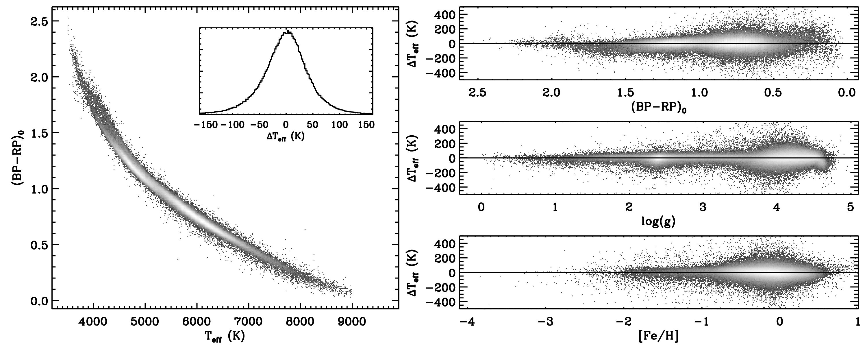
Figure 3: Left panel: log-density plot of the colour-$T_{\rm{eff}}$ relation obtained using all 360,000 GALAH DR3 stars with good photometric and spectroscopic flags as described in the text. For $T_{\rm{eff}}\lesssim 4500$ K the two loci defined by dwarf and giant stars can be noticed. The inset shows the distribution of the $T_{\rm{eff}}$ residuals of our calibration. Right panels: $T_{\rm{eff}}$ residuals plotted as function of colour, surface gravity and metallicity. Plots for the other colour indices are available as supplementary online material.

Depending on the combination of filters, there are over 360,000 stars available for our fits. We use only stars with $E(B-V)<0.1$ to derive our fits, to avoid a strong dependence on the adopted extinction law (Appendix B). Due to the combined effect of the GALAH selection function and target selection effects (most notably stellar evolutionary timescales), the distribution of targets has two main temperature overdensities: one at the main-sequence turn-off and the other at the red-clump phase. If all available stars were used to derive colour$-T_{\rm{eff}}$ relations these two overdensities would dominate the fit. Instead, we sample our stars uniformly in $T_{\rm{eff}}$, randomly selecting 20 stars every 20 K, and repeating this for 10 realizations. The calibration sample for each fit is thus based on roughly 50,000 stars. We repeat the above procedure 10,000 times, and select the fit that returns the lowest standard deviation with respect to the input effective temperatures from the IRFM. We also explored the effect of a uniform gridding in $T_{\rm{eff}}$ and $\log(g)$ but did not find any significant difference with respect to a uniform sampling in $T_{\rm{eff}}$ only.

To derive our relations we started with a polynomial as a function of colour, which is the parameter that has the strongest dependence on $T_{\rm{eff}}$. Depending on the colour index, we found that a third or fifth order polynomial was necessary to describe the curve inflection occurring at low $T_{\rm{eff}}$. We then added the [Fe/H] and $\log(g)$ dependence into the fit. The Gaia broad band filters have a rather mild dependence on metallicity, and the effect of $\log(g)$ is most noticeable below 4500 K, where colour-$T_{\rm{eff}}$ relations for dwarf and giant stars branch off (Figure 3 and 4). We found no need to go higher than first order in [Fe/H] and $\log(g)$, but cross-terms with colour, as well as a term involving colour, $T_{\rm{eff}}$ and $\log(g)$ were found to improve the fit. The adopted functional form is:

$$T_{\rm{eff}}=a_{0}+a_{1}X+a_{2}X^{2}+a_{3}X^{3}+a_{4}X^{5}+a_{5}\log(g)+a_{6}\log(g)\,X+$$

$$a_{7}\log(g)\,X^{2}+a_{8}\log(g)\,X^{3}+a_{9}\log(g)\,X^{5}+a_{10}\textrm{[Fe/H]}+$$

$$a_{11}\textrm{[Fe/H]}\,X+a_{12}\textrm{[Fe/H]}\,X^{2}+a_{13}\textrm{[Fe/H]}\,X^{3}+a_{14}\textrm{[Fe/H]}\log(g)\,X$$ (1)

where $X$ is the colour index corrected for reddening, and not all terms were found to be significant for all colour indices. The coefficients of Eq. 1 are given in Table 1. Our relations and associated standard deviations are derived over the range $3600\,\rm{K}\lesssim T_{\rm{eff}}\lesssim 9000$ K, although as we discuss in the next Section, they are validated by independent measurements over a smaller range of effective temperatures. Polynomial fits are also typically less robust towards the edges of a colour index. In Table 2 we recommend conservative colour ranges, which effectively limit the applicability of our relations between 4000 K and 8000 K for most filter combinations.

Table 2: Recommended colour range for the validity of our calibrations.

colour	dwarfs	giants
$(BP-RP)_{0}$	$[\phantom{+}0.20,\phantom{+}2.00]$	$[\phantom{+}0.20,\phantom{+}2.55]$
$(G-BP)_{0}$	$[-1.00,-0.15]$	$[-1.40,-0.15]$
$(G-RP)_{0}$	$[\phantom{+}0.15,\phantom{+}0.85]$	$[\phantom{+}0.15,\phantom{+}1.15]$
$(BP-J)_{0}$	$[\phantom{+}0.25,\phantom{+}3.00]$	$[\phantom{+}0.90,\phantom{+}4.20]$
$(BP-H)_{0}$	$[\phantom{+}0.40,\phantom{+}4.00]$	$[\phantom{+}0.40,\phantom{+}4.90]$
$(BP-K_{s})_{0}$	$[\phantom{+}0.30,\phantom{+}4.20]$	$[\phantom{+}0.30,\phantom{+}5.30]$
$(RP-J)_{0}$	$[\phantom{+}0.20,\phantom{+}1.05]$	$[\phantom{+}0.60,\phantom{+}1.55]$
$(RP-H)_{0}$	$[\phantom{+}0.20,\phantom{+}1.60]$	$[\phantom{+}0.20,\phantom{+}2.45]$
$(RP-K_{s})_{0}$	$[\phantom{+}0.20,\phantom{+}1.85]$	$[\phantom{+}0.20,\phantom{+}2.70]$
$(G-J)_{0}$	$[\phantom{+}0.15,\phantom{+}2.10]$	$[\phantom{+}1.00,\phantom{+}2.80]$
$(G-H)_{0}$	$[\phantom{+}0.25,\phantom{+}2.60]$	$[\phantom{+}0.25,\phantom{+}3.70]$
$(G-K_{s})_{0}$	$[\phantom{+}0.20,\phantom{+}2.80]$	$[\phantom{+}0.20,\phantom{+}3.90]$

Dwarfs and giants are separated as per Figure 4a.

Figure 3 shows the colour-$T_{\rm{eff}}$ relation for $(BP-RP)_{0}$, along with the residuals of the fit as function of colour, gravity and metallicity. Although Eq. (1) virtually allows for any combination of input parameters, it should be recalled that stars distribute across the HR diagram as permitted by stellar evolutionary theory. Figure 4a illustrates the range of stars used to build our colour calibrations, where cool stars are found both at low and high surface gravities, whilst the hottest stars have $\log(g)\sim 4$. Fig 4b and 4c show the dependence on $\log(g)$ and [Fe/H] for some of our colour-$T_{\rm{eff}}$ calibrations. In addition, to allow direct comparison, we also plot predictions from synthetic stellar fluxes computed with the bolometric-corrections code (Casagrande & VandenBerg, 2014, 2018). The purpose of this comparison is not to validate empirical nor theoretical relations, but to show that our functional form well captures the expected change of colours with $T_{\rm{eff}}$, $\log(g)$ and [Fe/H]. Some of the discrepancies between empirical and theoretical predictions at the coolest $T_{\rm{eff}}$ are likely due to inadequacies of synthetic fluxes as discussed in the literature (see e.g., Casagrande & VandenBerg, 2014; Böcek Topcu et al., 2020).

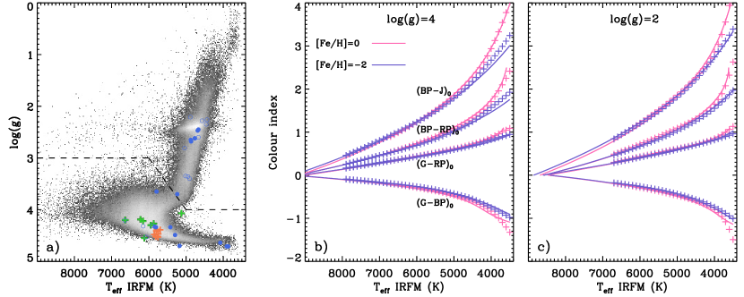
Figure 4: Panel a): Kiel diagram of the GALAH DR3 sample used to derive the colour-$T_{\rm{eff}}$ relations presented in this work. The dashed line marks the separation between dwarf and giant stars discussed in Section 4. Coloured crosses and circles are the stars used in Fig 6 to test the $T_{\rm{eff}}$ scale. Panel b) and c): some of the colour-$T_{\rm{eff}}$ relations (solid lines) of Table 1 for fixed values of $\log(g)=4$ and $\log(g)=2$, and $\textrm{[Fe/H]}=0$ and $\textrm{[Fe/H]}=-2$, as labelled. Plotted for comparison are synthetic colour-$T_{\rm{eff}}$ computed for the same values of gravity and metallicity (cross symbols). Note that the maximum $T_{\rm{eff}}$ available for synthetic colours varies with the adopted $\log(g)$.

4 Validation and uncertainties

We validate our colour-$T_{\rm{eff}}$ relations using three different test populations and approaches, focusing on Solar twins, Gaia Benchmark Stars (GBS), and interferometric measurements. The stars used for this purpose are some of the brightest and best observed in the sky, with careful determinations of their stellar parameters. In all instances, we apply the same requirements on phot_bp_rp_excess_factor and phot_proc_mode discussed in Section 3 to select the best photometry. We also exclude stars with $G<6$ and $BP$ and $RP<5$ due to uncalibrated systematics at bright magnitudes. We only use 2MASS photometry with Qflg=’A’ in a given band.

The sample of solar twins is the same that was used by Casagrande et al. (2010) to set the zero-point of their $T_{\rm{eff}}$ scale. These twins are all nearby, unaffected by reddening, and with good Gaia and 2MASS photometry. Accurate and precise spectroscopic $T_{\rm{eff}}$, $\log(g)$ and [Fe/H] are available from differential analysis of high-resolution, high S/N spectra with respect to a solar reference spectrum, using excitation and ionization balance of iron lines (Meléndez et al., 2006, 2009). In particular, the identification of the best twins is based on the measured relative difference in equivalent widths and equivalent widths vs. excitation potential relations with respect to the observed solar reference spectrum, and thus entirely model independent. In Table 3 we report the mean difference between the effective temperatures we derive in a given colour index, and the spectroscopic ones. Our $T_{\rm{eff}}$ are typically within few degrees of the spectroscopic ones. Further, regardless of the spectroscopic effective temperatures, the mean and median $T_{\rm{eff}}$ for our sample of solar twins in any colour index is always within few tens of K of the solar $T_{\rm{eff}}$. The fact that our colour-$T_{\rm{eff}}$ relations are well calibrated around the solar value is not unexpected, but confirms that we have achieved our goal of tying the current $T_{\rm{eff}}$ scale to that of Casagrande et al. (2010). To further test our scale, we use a large sample of more than 80 solar twins from Nissen (2015) and Spina et al. (2018). Also these twins have highly accurate and precise stellar parameters due to differential spectroscopic analysis. This means that in the comparison we are essentially dominated by photometric errors and intrinsic uncertainty in our colour-$T_{\rm{eff}}$ relations. The comparison in Figure 5 shows that the standard deviations for each colour index are consistent with the values reported in Table 1, although the latter are derived over a much larger range of stellar parameters. For solar type stars $(BP-RP)_{0}$, $(G-BP)_{0}$ and $(G-RP)_{0}$ are the colours with the highest precision, whilst the use of $RP$ photometry with 2MASS is the least informative, as it carries a typical uncertainty of order $100$ K. The standard error of the mean shows that individual colours can have systematic offsets of a few tens of K at most: although calibrations are built onto a set of input values, small local deviations are inherent to polynomial functional forms (see e.g., Ramírez & Meléndez, 2005). When deriving $T_{\rm{eff}}$ from colour relations, users should be mindful of the trade-off between choosing the colour index(es) with the highest precision versus using as many indices as possible to average down systematic errors (often at the cost of precision). If one were to use the mean $T_{\rm{eff}}$ from all indices, the mean difference with respect to the spectroscopic measurements in Figure 5 would be $4\pm 5$ K with a standard deviation $\sigma=48$ K.

For the GBS we use $T_{\rm{eff}},\log(g)$ and [Fe/H] from the latest version of the catalog (Jofré et al., 2018). The number of stars with good photometry varies depending on the filter used, with many of the GBS often having unreliable or saturated Gaia and/or 2MASS magnitudes. All GBS in our sample are closer than $\simeq 130$ pc, justifying the adoption of zero reddening. Again, we find overall excellent agreement between the $T_{\rm{eff}}$ we predict from colours, and those given in the GBS catalog.

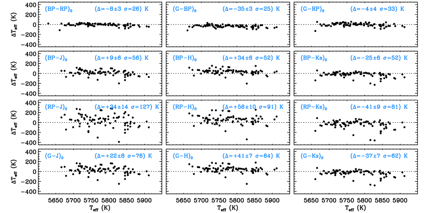
Figure 5: Comparison between the effective temperatures obtained from our calibrations and those derived by Nissen (2015) and Spina et al. (2018) from differential spectroscopic analysis of solar twins (x-axes). All targets are closer than 100pc and unaffected by reddening. In each panel we report the colour index used, the mean difference $\Delta(\rm{ours}-\rm{spectroscopy})$ $\pm$ standard error of the mean, and standard deviation ($\sigma$). Median and mean differences agree to within a few K.

Finally, we assemble a list of interferometric measurements from the recent literature: Bigot et al. (2011), Boyajian et al. (2012a, b), Huber et al. (2012), Maestro et al. (2013), White et al. (2013, 2018), Gallenne et al. (2018), Baines et al. (2018), Rains et al. (2020) and Karovicova et al. (2020). For all these stars, we adopt reddening, $\log(g)$ and [Fe/H] reported in the above papers. This list encompasses over 200 targets, although most of them are very bright, hence with unreliable Gaia and/or 2MASS magnitudes, reducing the sample usable for our comparison to at most thirty-three targets, depending on the colour index. For M dwarfs we only retain stars with $(BP-RP)_{0}\leq 2$ since this is roughly the reddest colour of dwarfs in GALAH DR3. Note that giant stars go to redder colours (up to $2.5$, cf. Figure 3), although interferometric $T_{\rm{eff}}$ of giants are available only for warmer temperatures. For the comparison in Table 3 we further require interferometric $T_{\rm{eff}}$ to be better than 1 percent, which is the target accuracy at which we aim in testing. Allowing for larger uncertainties results in an increase of scatter in the comparison, with a trend whereby interferometric $T_{\rm{eff}}$ are systematically cooler for those stars with the largest uncertainties. This is indicative that systematic errors tend to over-resolve angular diameters, hence under-predict effective temperatures (see discussion in Casagrande et al., 2014). Also, interferometric targets with the largest $T_{\rm{eff}}$ uncertainties are often affected by relatively high values of reddening, which adds to the error budget.

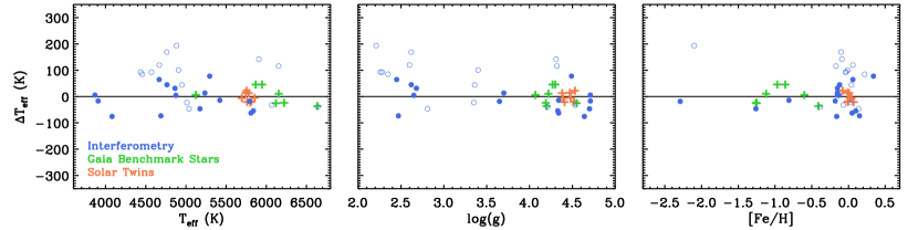
Figure 6: Comparison between $T_{\rm{eff}}$ derived using our $(BP-RP)_{0}$ relation and those available (ours$-$literature) for solar twins (orange), Gaia Benchmark Stars (blue) and interferometry (green). Filled and open circles indicate interferometric $T_{\rm{eff}}$ better than 1 and 2 percent, respectively.

Overall, it is clear from Table 3 that our relations are able to predict $T_{\rm{eff}}$ values in very good agreement with those reported in the literature for various benchmark samples. Depending on the colour index, mean differences are typically of order few tens of K. Occasional larger differences are still within the scatter of the relations, or are likely the result of small number statistics. When we restrict our analysis to the $(BP-RP)_{0}$ colour index, which has the largest number of stars available for comparison, the mean agreement is always within a few K regardless of the sample used (Figure 6).

Finally, we compare our relations against those of Mucciarelli & Bellazzini (2020), which are the only ones also available for dwarf and giant stars in the Gaia DR2 system. The colour-$T_{\rm{eff}}$ relations of Mucciarelli & Bellazzini (2020) are built using several hundred stars with $T_{\rm{eff}}$ derived from the IRFM work of González Hernández & Bonifacio (2009). For dwarf stars, the $T_{\rm{eff}}$ scale of González Hernández & Bonifacio (2009) agrees well with that of Casagrande et al. (2010, which underpins our study), with a nearly constant offset of $30-40$ K (our scale being hotter) due to the different photometric absolute calibrations adopted. The same offset is thus expected for Mucciarelli & Bellazzini (2020). This is explored in Figure 7, which shows the difference between the effective temperatures obtained using our relations against those of Mucciarelli & Bellazzini (2020) for colour indices in common. The first thing to notice is that the difference is not a constant offset, but varies as function of $T_{\rm{eff}}$, evolutionary status (dwarfs or giants) and colour index. To ensure this trend does not stem from the functional form of our polynomials, we have highlighted with filled circles stars for which our colour relations reproduce input $T_{\rm{eff}}$ from our IRFM to within 10 K. If one were to take the mean offset, it would typically be around few tens of K, with a maximum of order 50 K for $(G-RP)_{0}$ and $(G-BP)_{0}$, our scale being hotter. Overall, for most stars and colour indices, $T_{\rm{eff}}$ from our relations agree with those from Mucciarelli & Bellazzini (2020) to within $\sim 100$ K, which is the uncertainty expected when combining the precision (standard deviation) reported for both calibrations. Indices with short colour baseline like $(G-RP)_{0}$ or $(G-BP)_{0}$ display stronger systematic trends, in particular giants in $(G-BP)_{0}$. Larger deviations are also seen around and above 7000 K for dwarf stars, likely due to the paucity of hot stars available to Mucciarelli & Bellazzini (2020) to constrain well their calibration at high temperatures. Part of the trends might also arise from the fact than many of the calibrating giants in Mucciarelli & Bellazzini (2020) have $G<6$, a regime where Gaia DR2 photometry is affected by uncalibrated systematics. For our relations, we have also corrected the standardisation of Gaia DR2 $G$ magnitudes following Maíz Apellániz & Weiler (2018). Mucciarelli et al. (2021) provide updated relations using Gaia EDR3 photometry. As discussed in Appendix A, there are only minor differences between Figure 7 and 11 for $(BP-RP)_{0}$, $(BP-K_{s})_{0}$, $(RP-K_{s})_{0}$. This is not surprising, given the overall agreement of the colour-$T_{\rm{eff}}$ relations for Gaia DR2 and EDR3. However, indices involving $G$ magnitudes display reduced trends, which in part might arise from the better standardization of $G$ band photometry in EDR3.

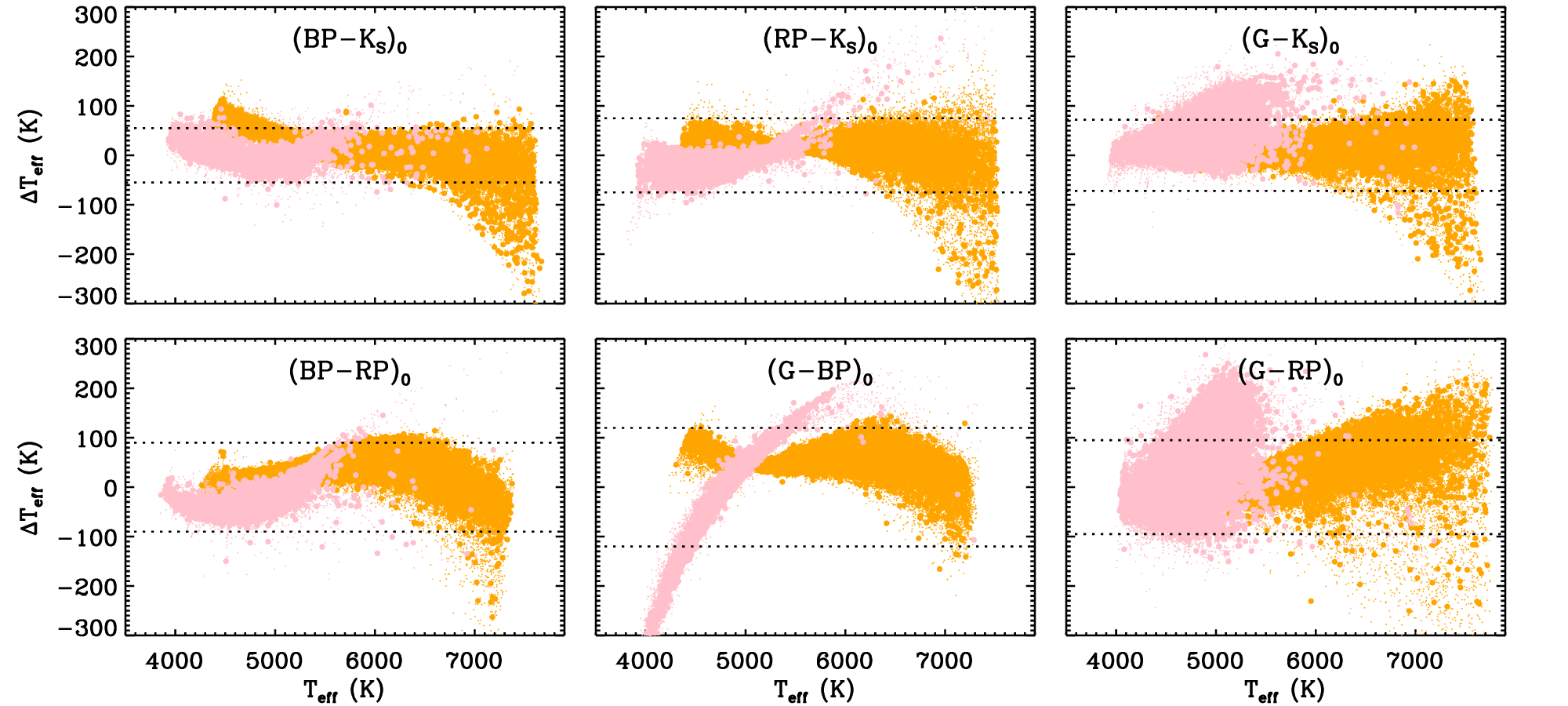
Figure 7: Comparison between $T_{\rm{eff}}$ derived using our relations and those of Mucciarelli & Bellazzini (2020, MB20) in the sense (ours$-$MB20). The relations of MB20 do not account for $\log(g)$, but are provided separately for dwarf (orange) and giant (pink) stars. Here, we use the separation (dwarfs vs. giants) defined by the dashed line of Figure 4 and apply the relations within their colour range. The same input [Fe/H] and dereddened photometry are used for both us and MB20. Filled circles are stars for which $T_{\rm{eff}}$ from our relations are within $10$ K of the IRFM, to ensure differences are not stemming from the functional form of our polynomials. Dotted lines are the squared root of the squared sum of the typical uncertainty quoted for each colour-$T_{\rm{eff}}$ relation.

From a user point of view, it is important to have realistic estimates of the precision at which $T_{\rm{eff}}$ can be estimated from our relations. In Table 1, we report two values for the standard deviation of our colour-$T_{\rm{eff}}$ relations. The first value is the precision of the fits. The second provides a more realistic assessment of the uncertainties encountered when applying our relations, and is obtained by randomly perturbing the input [Fe/H] and $\log(g)$ with a Gaussian distribution of width $0.2$ and $0.5$ dex, respectively. The effect of a systematic shift of the GALAH $\log(g)$ and [Fe/H] scale by $\pm 0.2$ and $\pm 0.1$ dex respectively is typically also of a few tens of K at most. It should be kept in mind that uncertainties in the input stellar parameters will propagate differently with different colours, the effect being strongest for the coolest stars. Users of our calibrations are encouraged to assess their uncertainties on a case-by-case basis, by propagating the errors in their input parameters through Eq. 1. Further, an extra uncertainty of 20 K should still be added to account for the zero-point uncertainty of our $T_{\rm{eff}}$ scale (from Casagrande et al. 2010, see discussion in Section 2). We provide the code colte to derive $T_{\rm{eff}}$ from our colour relations, taking into account the applicability ranges of Table 2, and with the option to derive realistic uncertainties through a MonteCarlo for each colour index. Other notable options include the choice of different extinction laws, and Gaia DR2 or EDR3 photometry.

Although our calibrations take into account the effect of surface gravity, there might be instances where the input $\log(g)$ is not known, besides a rough “dwarf” vs “giant” classification. To assess this impact, we classify stars as dwarfs (giants) if their gravities are higher (lower) than the dashed line of Figure 4a. We then adopt a constant $\log(g)=4$ for dwarfs and $\log(g)=2$ for giants. The effect of such an assumption on the derived $T_{\rm{eff}}$ is typically small, as can be seen in Figure 8. The largest differences occur for stars in the upper giant branch, where assuming a constant $\log(g)=2$ becomes inappropriate for $\log(g)\lesssim 1-1.5$. This effect can be quite strong for certain colour indices. In this case, one might use the fact that there is a strong correlation between the intrinsic colour and the surface gravity of stars along the RGB for a better assignment of $\log(g)$.

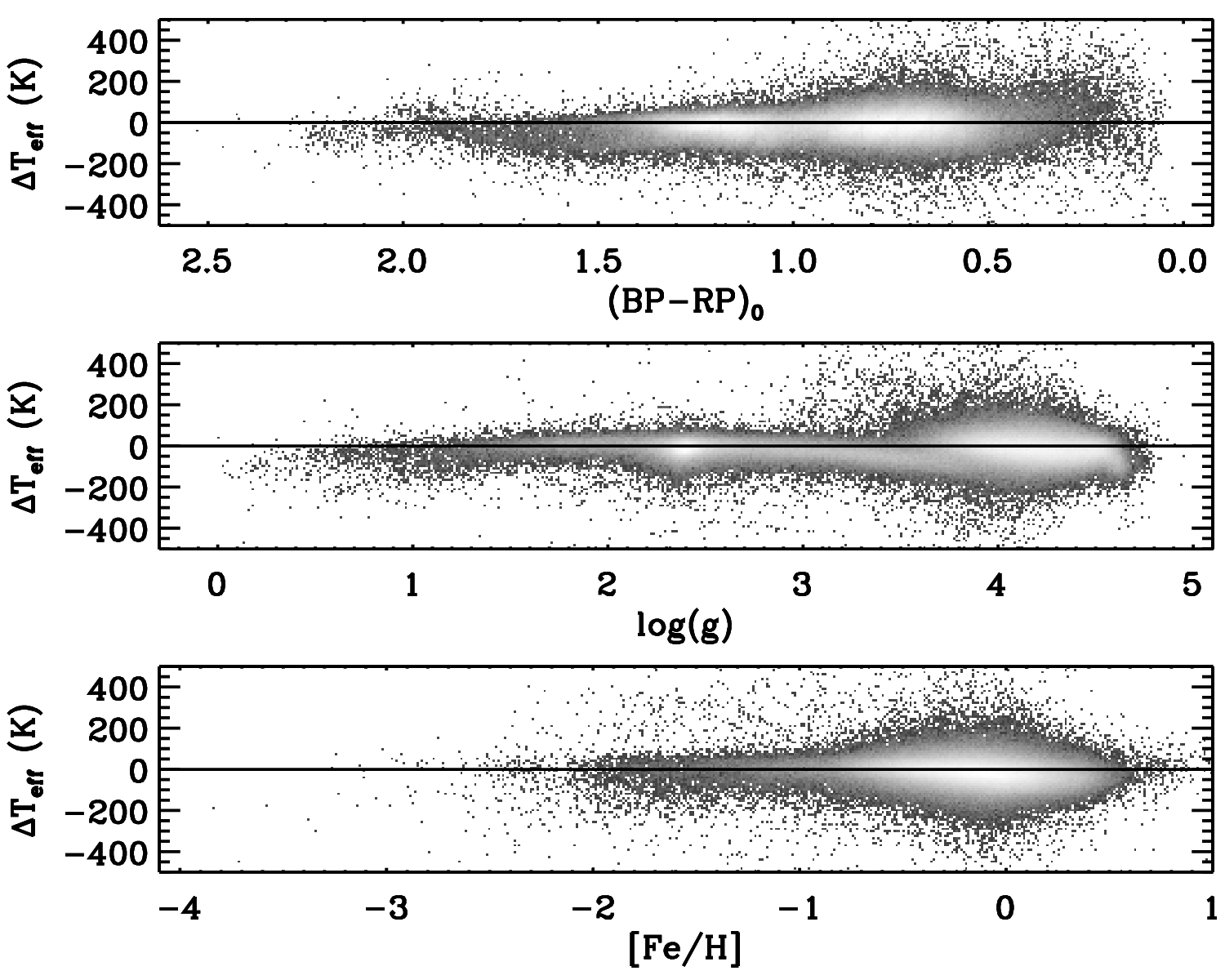
Figure 8: $T_{\rm{eff}}$ residual for the $(BP-RP)_{0}$ calibration when stars are assigned a fixed $\log(g)=2$ or $4$ based on their classification as giants or dwarfs as per Figure 4. Plots for the other colour indices are available as supplementary online material.

Table 3: Mean difference and standard deviation between the effective temperatures derived from our calibrations, and those from the literature used for validation (ours$-$literature). $N$ is the number of stars available in each colour index.

colour	Solar Twins		GBS		Interferometry†
	$\langle\Delta T_{\rm{eff}}\rangle$	N	$\langle\Delta T_{\rm{eff}}\rangle$	N	$\langle\Delta T_{\rm{eff}}\rangle$	N
$(BP-RP)_{0}$	$-3\pm 17$	8	$3\pm 34$	7	$-8\pm 49$	15
$(G-BP)_{0}$	$-30\pm 16$	8	$-19\pm 42$	5	$-10\pm 68$	7
$(G-RP)_{0}$	$0\pm 22$	8	$10\pm 31$	5	$-12\pm 55$	7
$(BP-J)_{0}$	$-6\pm 23$	8	$10\pm 55$	5	$9\pm 48$	3
$(BP-H)_{0}$	$10\pm 13$	8	$49\pm 48$	5	$95\pm 8$	2
$(BP-K_{s})_{0}$	$-14\pm 21$	8	$-16\pm 32$	6	$-30\pm 60$	6
$(RP-J)_{0}$	$-13\pm 69$	8	$2\pm 108$	5	$-42\pm 112$	3
$(RP-H)_{0}$	$-2\pm 36$	8	$25\pm 74$	5	$68\pm 14$	2
$(RP-K_{s})_{0}$	$-28\pm 37$	8	$-52\pm 40$	6	$-51\pm 59$	6
$(G-J)_{0}$	$-2\pm 36$	8	$-4\pm 72$	5	$-16\pm 49$	3
$(G-H)_{0}$	$5\pm 20$	8	$18\pm 59$	5	$60\pm 50$	2
$(G-K_{s})_{0}$	$-27\pm 26$	8	$-52\pm 40$	5	$-54\pm 74$	5

^†Only interferometric $T_{\rm{eff}}$ better than 1 percent are used.

5 Conclusions

In this paper we have implemented the Gaia DR2 and EDR3 photometric system in the IRFM and applied to over 360,000 stars with good spectroscopic and photometric flags to derive $T_{\rm{eff}}$ for stars across different evolutionary phases. In the literature, colour-$T_{\rm{eff}}$ relations for late type-stars are typically given separately for dwarfs and giants. The advent of Gaia parallaxes allows us to use robust surface gravities together with [Fe/H] from the GALAH DR3 survey to provide colour-$T_{\rm{eff}}$ relations that take into account the effect of these two parameters. Our calibrations are built and tested using the largest high-resolution stellar spectroscopic survey to date and cover a wide range of stellar colours and parameters: $0\lesssim\log(g)\lesssim 4.8$ and $-3\lesssim\textrm{[Fe/H]}\lesssim 0.6$. When using our relations, users should refer to Figures 3 and 4 to have a sense for the parameter space covered, and for the performances of different colour indices. Users should always be mindful of the trade-off between choosing the colour index(es) with the highest precision versus using as many indices as possible to average down systematic errors, often at the cost of precision. $(BP-K_{s})_{0}$ and $(G-K_{s})_{0}$ are the indices which are best calibrated against $T_{\rm{eff}}$ across the parameter space, whereas indices leveranging on $RP$ are the least performing ones. In particular, $(RP-J)_{0}$ has a very short colour baseline and the largest scatter, and other colour indices should be used instead, if possible. Moving to indices built only with Gaia filters, $(BP-RP)_{0}$ is the best choice, although $(G-BP)_{0}$ and $(G-RP)_{0}$ are also informative. For solar twins, all three indices return $T_{\rm{eff}}$ with remarkably small scatter with respect to the highly precise ones derived from differential spectroscopic analyses. Robust solar colours have also been derived (Appendix C). For most colour indices, our calibrations have a typical 1 sigma uncertainty of $40-80$ K for the colour intervals of Table 2, which cover the region between 4000 K and 8000 K. For $4000\,\rm{K}\lesssim T_{\rm{eff}}\lesssim 6700$ K our calibrations are also validated against solar twins, Gaia Benchmark Stars and interferometry.

Data availability

The data underlying this article were accessed from the GALAH survey DR3 which can be queried using TAP at https://datacentral.org.au/vo/tap. The derived data generated in this research will be shared on reasonable request to the corresponding author.

Table 1: Coefficients of the $T_{\rm{eff}}$ calibration of Eq. 1 suitable for Gaia DR2 photometry. See Appendix A for Gaia EDR3 photometry.

colour	$a_{0}$	$a_{1}$	$a_{2}$	$a_{3}$	$a_{4}$	$a_{5}$	$a_{6}$	$a_{7}$	$a_{8}$	$a_{9}$	$a_{10}$	$a_{11}$	$a_{12}$	$a_{13}$	$a_{14}$	$\sigma(T_{\rm{eff}})$ (K)
$(BP-RP)_{0}$	$7928$	$-3663.1140$	$803.3017$	$-9.3727$	$-$	$325.1324$	$-500.1160$	$279.4832$	$-53.5062$	$-$	$-2.4205$	$-128.0354$	$49.4933$	$5.9146$	$41.3650$	$54-66$
$(G-BP)_{0}$	$7555$	$5803.7715$	$-$	$-2441.7124$	$437.7314$	$455.0997$	$2243.1333$	$3669.4924$	$1872.7035$	$-$	$19.1085$	$75.2198$	$-$	$-$	$-83.9777$	$75-93$
$(G-RP)_{0}$	$7971$	$-5737.5049$	$-$	$1619.9946$	$-203.8234$	$255.7408$	$-492.8268$	$160.1957$	$103.1114$	$-$	$-64.3289$	$34.3339$	$-$	$-$	$54.7224$	$56-64$
$(BP-J)_{0}$	$8218$	$-2526.8430$	$458.1827$	$-28.4540$	$-$	$234.0113$	$-205.3084$	$63.4781$	$-7.2083$	$-$	$-85.7048$	$-50.1557$	$32.3428$	$-2.3553$	$20.0671$	$44-49$
$(BP-H)_{0}$	$8462$	$-2570.3684$	$537.5968$	$-44.3644$	$-$	$189.1198$	$-106.7584$	$31.1720$	$-4.9137$	$-$	$-9.2587$	$-189.8600$	$75.8619$	$-6.8592$	$16.7226$	$33-42$
$(BP-K_{s})_{0}$	$8404$	$-2265.1355$	$403.4693$	$-27.9056$	$-$	$193.5820$	$-145.3724$	$47.7998$	$-6.4572$	$-$	$-34.5438$	$-130.2559$	$52.6470$	$-4.4777$	$15.8249$	$24-32$
$(RP-J)_{0}$	$9074$	$-7670.6606$	$3164.0525$	$-$	$-126.1476$	$-$	$-7.3816$	$-12.5168$	$-$	$-2.0452$	$-$	$76.1144$	$-$	$-$	$-45.8056$	$90-95$
$(RP-H)_{0}$	$8924$	$-4779.3394$	$1319.8989$	$-$	$-16.6676$	$-$	$-23.6583$	$22.4243$	$-$	$-4.3066$	$-$	$35.0102$	$-$	$-$	$-28.7228$	$52-62$
$(RP-K_{s})_{0}$	$8940$	$-4450.6138$	$1138.6816$	$-$	$-10.5749$	$-$	$-42.3037$	$33.3365$	$-$	$-3.2535$	$-$	$41.0402$	$-$	$-$	$-21.9922$	$43-48$
$(G-J)_{0}$	$8370$	$-3559.7710$	$895.8869$	$-86.7011$	$-$	$180.7568$	$-164.9264$	$24.4263$	$4.2318$	$-$	$-127.9640$	$72.1449$	$-$	$-$	$13.7683$	$54-57$
$(G-H)_{0}$	$8186$	$-2536.7671$	$503.2762$	$-42.7871$	$-$	$230.4871$	$-254.5291$	$104.6258$	$-17.4859$	$-$	$-122.0732$	$45.0572$	$-$	$-$	$6.9992$	$37-41$
$(G-K_{s})_{0}$	$8103$	$-1857.7194$	$-$	$73.1834$	$-1.7576$	$236.0335$	$-345.9070$	$170.4915$	$-28.8549$	$-$	$-131.4548$	$49.6232$	$-$	$-$	$10.0777$	$27-32$

$G$ magnitudes have been corrected following Maíz Apellániz & Weiler (2018): $G+0.0271\,(6-G)$ for $G\leq 6$, $G-0.0032\,(G-6)$ for $6<G<16$ and $G-0.032$ for $G\geq 16$. These corrections should be applied before using our relations with $G$ magnitudes: the effect on indices with short colour baseline such as $(G-BP)_{0}$ and $(G-RP)_{0}$ is noticeable, and up to $100-200$ K for hot stars in particular. See Table 3 for extinction coefficients suitable for Gaia DR2 and 2MASS. Users should also be wary of applying colour-$T_{\rm{eff}}$ relations to stars with $G<6$ and $BP$ and $RP$ brighter than $\sim 5$ due to the saturation of bright magnitudes in Gaia. For the standard deviation of the calibration $\sigma(T_{\rm{eff}})$, we provide two estimates, both obtained using all available $\sim 360,000$ stars, instead of the $\sim 50,000$ used to derive fits. The first one is the precision of the fits, whereas for the second one input [Fe/H] and $\log(g)$ are perturbed with a Gaussian random noise of $0.2$ and $0.5$ dex, respectively. Note that an extra uncertainty of about 20 K on the zero-point of our effective temperature scale should still be added.

Appendix A Colour-$T_{\rm{eff}}$ relations using Gaia EDR3 photometry

The IRFM and colour-$T_{\rm{eff}}$ relations described in the paper are based on Gaia DR2 photometry. Here we discuss the implementation of Gaia EDR3 photometry into the IRFM and provide colour-$T_{\rm{eff}}$ relations for this system.

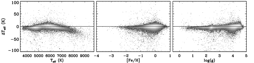
Figure 9: Log-density plot of the difference in effective temperatures derived by the IRFM when implementing Gaia EDR3 photometry instead of DR2 in the optical (EDR3 minus DR2). Approximately 355,000 stars with good GALAH spectroscopic, and photometric flags in both EDR3 and DR2 are shown here. For 96 percent of the stars the difference is always within $\pm 10$ K.

Gaia EDR3 photometry defines an independent photometric system from Gaia DR2, with significant improvements in the processing of the data and photometric calibration (see Riello et al., 2021, for an in depth discussion). These improvements affect not only the published EDR3 magnitudes (and fluxes), but also the filter transmission curves and zero-points defining the system. Here, we implement EDR3 passbands and zero-points, along with EDR3 $BP$ and $RP$ photometry into the IRFM. As described in Section 2, 2MASS $JHK_{s}$ are used in the infrared. Also in this instance we do not use the redundant information from EDR3 $G$ magnitudes in the IRFM, although we do provide calibrations involving this band. $BP$, $RP$ and $G$ magnitudes for bright sources have been corrected for saturation effects following Riello et al. (2021). $G$ magnitude correction for bright blue sources is not applied since none of our target is bluer than $BP-RP\sim 0$, but we correct $G$ magnitudes for sources with 2 or 6-parameter astrometric solutions.

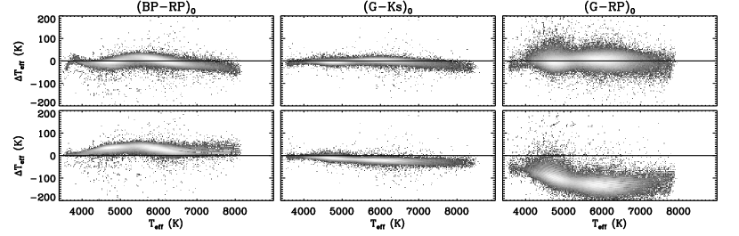
Figure 10: Top panels: log-density plots of the effective temperature difference between the Gaia EDR3 and DR2 calibration when photometry from the corresponding release is used. Bottom panels: effective temperature difference between using both EDR3 and DR2 photometry into the EDR3 calibration. The offset in $(G-RP)_{0}$ largely originates from the correction applied to DR2 $G$ magnitudes (see discussion in the text). In all instances, calibrations have been applied within the validity ranges of Table 2.

As in Section 2, we derive $T_{\rm{eff}}$ for all stars in Casagrande et al. (2010) with a counterpart in EDR3 (now 410 targets), obtaining a mean and median $\Delta T_{\rm{eff}}=17\pm 2$ K ($\sigma=41$ K). The mean $T_{\rm{eff}}$ difference of implementing Gaia EDR3 instead of DR2 photometry is a mere 5K with a slight trend as function of $T_{\rm{eff}}$. The latter is more clearly visible when comparing effective temperatures obtained from the IRFM for the entire GALAH sample (Figure 9). For 96 (99) percent of stars the difference is always within $\pm 10$ K ($\pm 20$ K), well within the zero-point uncertainty of our scale, and no noticeable trends with surface gravity and metallicity. Above 7500 K however there is the tendency for EDR3 to return effective temperatures which are systematically cooler by some tens of K.

Table 2 provides colour-$T_{\rm{eff}}$ coefficients derived in a similar fashion to Table 1, but using instead EDR3 photometry. We select good photometry by requesting phot_proc_mode=0 and $BP$ and $RP$ corrected excess factor $-0.08<C^{\star}<0.2$ (Riello et al., 2021). This last requirement is similar to $0.001+0.039\,(BP-RP)<\log_{10}({\tt phot\_bp\_rp\_excess\_factor})<0.12+0.039\,(BP-RP)$ used by Gaia Collaboration et al. (2021) to select good photometry. Note that extinction coefficients for Gaia EDR3 filters are also updated from Figure 1, and provided in Table 3.

It is important to note that although the calibration for Gaia DR2 and EDR3 are overall similar, photometry from one system should never be used with the calibration of the other. The danger of doing this is shown for a few selected colour combinations in Figure 10. On the top panels, when photometry from a data release is used with its colour-$T_{\rm{eff}}$ relation, the agreement between effective temperatures is consistent to what expected from Figure 9 (as calibrations in different indices have their own intrinsic scatter). However, if -say- photometry from DR2 is used onto the calibration for EDR3 (equivalent of plotting the difference of the relations at same colour), systematic offsets will appear. This is particularly relevant for indices involving $G$ magnitudes, which for Gaia DR2 have been corrected following Maíz Apellániz & Weiler (2018). Although this correction is magnitude dependent, over the range of our stars it amounts to few hundredths of a magnitude. This difference does not significantly impact $T_{\rm{eff}}$ in colours with long baseline, see e.g., $(G-K_{s})_{0}$ in the bottom mid panel of Figure 10. However, for indices like $(G-BP)_{0}$ or $(G-RP)_{0}$, effective temperatures can be off by as much as $100-200$ K (bottom right panel of Figure 10).

Although $G$ magnitudes for sources with 2 or 6-parameter astrometric solutions still need minor corrections in EDR3, zero-point shifts to improve standardisation are not necessary anymore (cf. Casagrande & VandenBerg, 2018; Maíz Apellániz & Weiler, 2018, for Gaia DR2). Similarly, many of the bright objects used by Mucciarelli et al. (2021) to define their relations have much improved $G$ band photometry in EDR3. This likely explains the reduced trends when comparing our EDR3 calibrations against those of Mucciarelli et al. (2021) for indices involving $G$ band (see Figure 11 and discussion in Section 4).

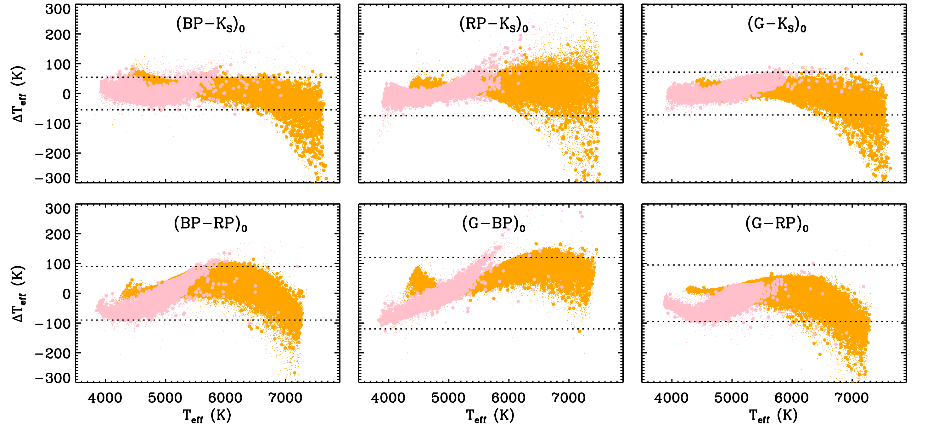
Figure 11: Same as Figure 7, but comparing our Gaia EDR3 relations against those of Mucciarelli et al. (2021).

Table 2: Coefficients of the $T_{\rm{eff}}$ calibration of Eq. 1 suitable for Gaia EDR3 photometry.

colour	$a_{0}$	$a_{1}$	$a_{2}$	$a_{3}$	$a_{4}$	$a_{5}$	$a_{6}$	$a_{7}$	$a_{8}$	$a_{9}$	$a_{10}$	$a_{11}$	$a_{12}$	$a_{13}$	$a_{14}$	$\sigma(T_{\rm{eff}})$ (K)
$(BP-RP)_{0}$	$7981$	$-4138.3457$	$1264.9366$	$-130.4388$	$-$	$285.8393$	$-324.2196$	$106.8511$	$-4.9825$	$-$	$4.5138$	$-203.7774$	$126.6981$	$-14.7442$	$40.7376$	$55-64$
$(G-BP)_{0}$	$7346$	$5810.6636$	$-$	$-2880.3823$	$669.3810$	$415.3961$	$2084.4883$	$3509.2200$	$1849.0223$	$-$	$-49.0748$	$6.8032$	$-$	$-$	$-100.3419$	$76-88$
$(G-RP)_{0}$	$8027$	$-5796.4277$	$-$	$1747.7036$	$-308.7685$	$248.1828$	$-323.9569$	$-120.2658$	$225.9584$	$-$	$-35.8856$	$-16.5715$	$-$	$-$	$48.5619$	$53-61$
$(BP-J)_{0}$	$8172$	$-2508.6436$	$442.6771$	$-25.3120$	$-$	$251.5862$	$-240.7094$	$86.0579$	$-11.2705$	$-$	$-45.9166$	$-137.4645$	$75.3191$	$-8.7175$	$21.5739$	$44-49$
$(BP-H)_{0}$	$8159$	$-2146.1221$	$368.1630$	$-24.4624$	$-$	$231.8680$	$-170.8788$	$52.9164$	$-6.8455$	$-$	$-45.5554$	$-142.9127$	$55.2465$	$-4.1694$	$17.6593$	$32-40$
$(BP-K_{s})_{0}$	$8266$	$-2124.5574$	$355.5051$	$-23.1719$	$-$	$209.9927$	$-161.4505$	$50.5904$	$-6.3337$	$-$	$-27.2653$	$-160.3595$	$67.9016$	$-6.5232$	$16.5137$	$24-33$
$(RP-J)_{0}$	$9047$	$-7392.3789$	$2841.5464$	$-$	$-85.7060$	$-$	$-88.8397$	$80.2959$	$-$	$-15.3872$	$-$	$54.6816$	$-$	$-$	$-32.9499$	$91-93$
$(RP-H)_{0}$	$8871$	$-4702.5469$	$1282.3384$	$-$	$-15.8164$	$-$	$-30.1373$	$27.9228$	$-$	$-4.8012$	$-$	$25.1870$	$-$	$-$	$-22.3020$	$52-59$
$(RP-K_{s})_{0}$	$8911$	$-4305.9927$	$1051.8759$	$-$	$-8.6045$	$-$	$-76.7984$	$55.5861$	$-$	$-3.9681$	$-$	$35.4718$	$-$	$-$	$-16.4448$	$43-46$
$(G-J)_{0}$	$8142$	$-3003.2988$	$499.1325$	$-4.8473$	$-$	$244.5030$	$-303.1783$	$125.8628$	$-18.2917$	$-$	$-125.8444$	$59.5183$	$-$	$-$	$16.8172$	$53-56$
$(G-H)_{0}$	$8134$	$-2573.4998$	$554.7657$	$-54.0710$	$-$	$229.2455$	$-206.8658$	$68.6489$	$-10.5528$	$-$	$-124.5804$	$41.9630$	$-$	$-$	$7.9258$	$36-41$
$(G-K_{s})_{0}$	$8032$	$-1815.3523$	$-$	$70.7201$	$-1.7309$	$252.9647$	$-342.0817$	$161.3031$	$-26.7714$	$-$	$-120.1133$	$42.6723$	$-$	$-$	$10.0433$	$27-31$

Refer to Table 1 for a description of the columns. The same colour limits given in Table 2 apply here. Before using these relations, $G,BP$ and $RP$ magnitudes for bright sources needs to be corrected for saturation. For sources with 2 or 6-parameter astrometric solutions $G$ magnitudes must also be corrected (Riello et al., 2021). See Table 3 for extinction coefficients suitable for Gaia EDR3 and 2MASS.

Appendix B The dependence of colour-$T_{\rm{eff}}$ relations on the adopted extinction law

The relations of Table 1 and 2 have been derived adopting the Cardelli et al. (1989)/O’Donnell (1994) extinction law (hereafer COD) for consistency with our earlier work on the IRFM (Casagrande et al., 2010). Here, we investigate the effect of using a different extinction law, namely that of Fitzpatrick (1999), renormalized as per Schlafly & Finkbeiner (2011, hereafter referred to as FSF). Changing law affects the amount of extinction inferred in each photometric band for a given input $E(B-V)$. In other words, different extinction coefficients will be derived. This is due to the fact that extinction laws have different normalizations and shapes. Because of the normalization, extinction coefficients will be higher or lower by a similar percent. Because of the shape, certain photometric bands will be affected more than others in relative terms. Changes in normalization and shape of extinction laws can also be due to variations in $R_{V}$ (i.e. the ratio of total to selective extinction in $V$ band, used to build a one-parameter family of curves). In this work, however, we adopt the “standard” $R_{V}=3.1$ which applies to the diffuse interstellar medium for most line of sights in the Galaxy.

Depending on the extinction law, different unreddened colours will be obtained for the same input reddening, thus affecting photometric effective temperatures. The extinction coefficients derived with FSF are roughly 15 to 25 percent lower than with COD, implying that $T_{\rm{eff}}$ of stars affected by reddening will be cooler assuming the former extinction law (Table 3). This is shown in the left panel of Figure 12, which compares $T_{\rm{eff}}$ derived using the COD or the FSF law into the IRFM. For the highest reddening values in our sample the difference in temperature can reach up to $\sim$10 percent, which corresponds to several hundreads of K for hot stars. Fortunately, the effect on the colour-$T_{\rm{eff}}$ relations is much smaller. For low reddening values (central panel of Figure 12), bluer or redder stellar colours map into hotter or cooler effective temperature, roughly moving on the same colour-$T_{\rm{eff}}$ relation, regardless of the underlying extinction law. Thus, even if our relations have been derived using the COD law, a change of extinction coefficients suffices to derive effective temperatures under different extinction curves. This has been verified by using the coefficients in Table 3 with the calibrations of Table 1 and 2: within the precision allowed by our colour-$T_{\rm{eff}}$ relations, we are able to recover $T_{\rm{eff}}$ when the COD or FSD law is implemented in the IRFM directly.

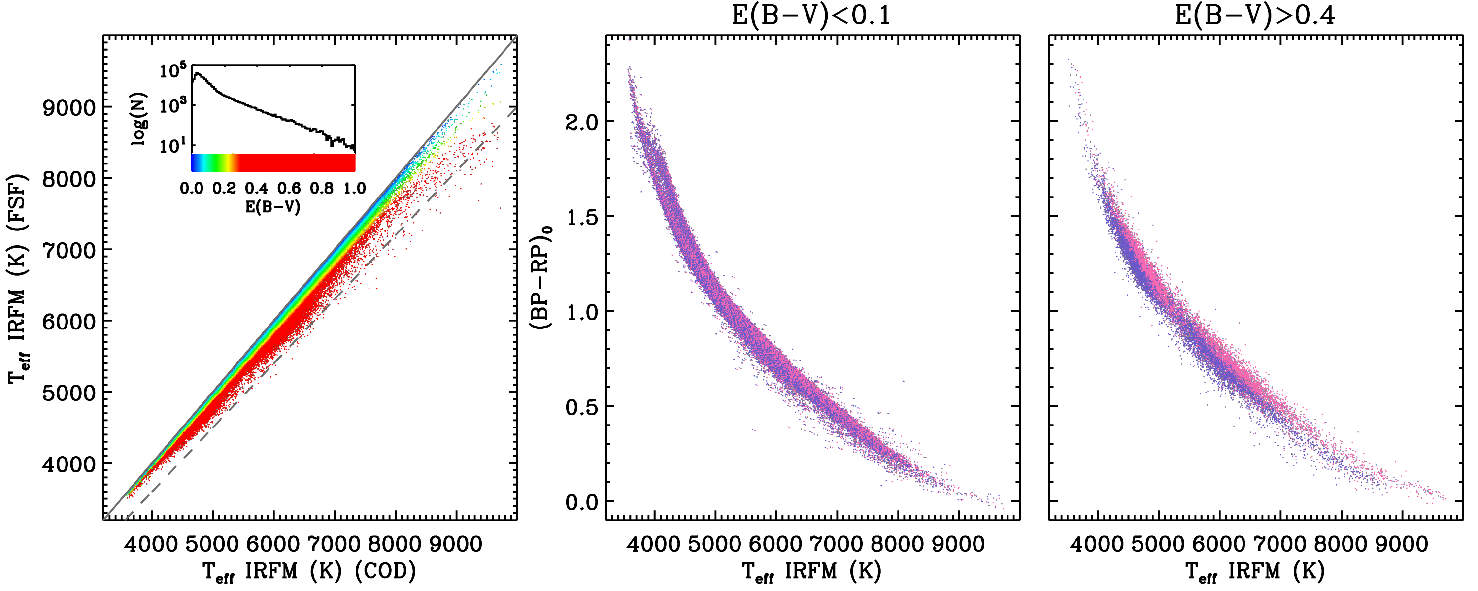
Figure 12: Left panel: comparison between $T_{\rm{eff}}$ obtained implementing the COD or the FSF extinction law in the IRFM. Stars are colour-coded by their $E(B-V)$ with the distribution shown in the inset. Continuous grey line is the one-to-one relation, whereas the dashed line marks a 10 percent decrease in $T_{\rm{eff}}$. Central panel: colour-$T_{\rm{eff}}$ derived using the COD (pink) and the FSF (purple) extinction laws when reddening is below $0.1$. Right panel: same as central panel, but when reddening is above $0.4$.

Table 3: Colour dependent extinction coefficients $R_{\zeta}=b_{0}+b_{1}(BP-RP)_{0}+b_{2}(BP-RP)_{0}^{2}+b_{3}(BP-RP)_{0}^{3}$ for Gaia and 2MASS photometry assuming different laws. To estimate intrinsic colours needed for the fits, one can iterate starting with the assumption $(BP-RP)_{0}\simeq(BP-RP)-E(B-V)$.

	COD extinction law								FSF extinction law
	Gaia DR2				Gaia EDR3				Gaia DR2				Gaia EDR3
	$b_{0}$	$b_{1}$	$b_{2}$	$b_{3}$	$b_{0}$	$b_{1}$	$b_{2}$	$b_{3}$	$b_{0}$	$b_{1}$	$b_{2}$	$b_{3}$	$b_{0}$	$b_{1}$	$b_{2}$	$b_{3}$
$R_{G}$	$3.068$	$-0.504$	$0.053$	$-$	$3.071$	$-0.511$	$0.058$	$-$	$2.608$	$-0.468$	$0.048$	$-$	$2.609$	$-0.475$	$0.053$	$-$
$R_{BP}$	$3.533$	$-0.114$	$-0.219$	$0.070$	$3.526$	$-0.168$	$-0.170$	$0.060$	$3.007$	$-0.099$	$-0.212$	$0.069$	$2.998$	$-0.140$	$-0.175$	$0.062$
$R_{RP}$	$2.078$	$-0.073$	$-$	$-$	$2.062$	$-0.072$	$-$	$-$	$1.702$	$-0.060$	$-$	$-$	$1.689$	$-0.059$	$-$	$-$
$R_{J}$	$0.899$	$-$	$-$	$-$	$0.899$	$-$	$-$	$-$	$0.719$	$-$	$-$	$-$	$0.719$	$-$	$-$	$-$
$R_{H}$	$0.567$	$-$	$-$	$-$	$0.567$	$-$	$-$	$-$	$0.455$	$-$	$-$	$-$	$0.455$	$-$	$-$	$-$
$R_{K_{s}}$	$0.366$	$-$	$-$	$-$	$0.366$	$-$	$-$	$-$	$0.306$	$-$	$-$	$-$	$0.306$	$-$	$-$	$-$

See discussion in Appendix B for the definition of COD and FSF extinction laws.

Appendix C Solar colours

By fixing the solar surface gravity, metallicity and effective temperature, Eq. 1 can be solved to derive the colours of the Sun. Here we adopt $\log(g)_{\odot}=4.44$ and $T_{\rm{eff},\odot}=5777$ K, where the latter value is kept for consistency with our previous sets of solar colours (Casagrande et al., 2010, 2012) We verified however that if we were to adopt the effective temperature recommended by the IAU 2015 Resolution B3 (5772 K, Prša et al., 2016) the derived colours would change at most by $0.004$ mag, which is considerably less than our uncertainties (where a lower $T_{\rm{eff},\odot}$ implies redder solar colours).

In Table 4 we report the colours derived from Table 1 and 2 for the Gaia DR2 and EDR3 system, respectively. The precision $\sigma(T_{\rm{eff}})$ quoted for our colour-$T_{\rm{eff}}$ relations is used to perturb $T_{\rm{eff},\odot}$, and to derive uncertainties for the colours of the Sun. The 20 K uncertainty on the zero-point of our effective temperature scale is not included, and it would typically imply a systematic shift to our colours of order 0.01 mag, depending on the index.

For comparison we also derive solar colours using four high fidelity, flux calibrated spectra (from Rieke et al. 2008, the CALSPEC solar reference spectrum sun_reference_stis_002, and the solar irradiance spectra of Thuillier et al. 2004 and Meftah et al. 2018). The zero-points and transmission curves used to compute colours from these spectra are the same we have adopted in the IRFM for the Gaia DR2, EDR3 and 2MASS system. The agreement between the colours derived from these four spectra is usually very good, the standard deviation being always below $0.008$ mag for all indices, except for those involving the $H$ and $K_{s}$ band (where the standard deviation increases to $0.02-0.04$ mag).

Figure 13 shows that our inferred solar colours are in overall excellent agreement with those obtained from solar reference spectra and solar twins. We use the same solar twins of Table 3, which have an average spectroscopic $T_{\rm{eff}}$ centred within couple of K from our adopted solar value (depending whether the sample from DR2 -which comprises 8 stars- or EDR3 -10 stars- is used). For the Gaia DR2 system, colours map the effective temperature differences already discussed for Table 3. It can be appreciated how well the colours of the Sun from different dataset agree, the difference being $\lesssim 0.02$ mag for virtually all bands. In the EDR3 system, the agreement is particularly remarkable for the pure Gaia colours $(BP-RP)_{0}$, $(G-BP)_{0}$ and $(G-RP)_{0}$, where our temperature scale, solar twins and solar spectra all agree to better than $0.006$ mag. This is likely indicative of how well EDR3 zero-points and transmission curves are characterized, and how robustly solar colours can now be derived for the Gaia system.

Table 4: Solar colours.

colour	Gaia DR2 - 2MASS	Gaia EDR3 - 2MASS
$(BP-RP)_{0}$	$0.823\pm 0.018$	$0.815\pm 0.018$
$(G-BP)_{0}$	$-0.354\pm 0.012$	$-0.322\pm 0.011$
$(G-RP)_{0}$	$0.465\pm 0.009$	$0.489\pm 0.009$
$(BP-J)_{0}$	$1.372\pm 0.025$	$1.350\pm 0.025$
$(BP-H)_{0}$	$1.683\pm 0.025$	$1.660\pm 0.024$
$(BP-K_{s})_{0}$	$1.731\pm 0.019$	$1.712\pm 0.018$
$(RP-J)_{0}$	$0.549\pm 0.021$	$0.538\pm 0.021$
$(RP-H)_{0}$	$0.852\pm 0.020$	$0.843\pm 0.020$
$(RP-K_{s})_{0}$	$0.907\pm 0.018$	$0.895\pm 0.018$
$(G-J)_{0}$	$1.016\pm 0.022$	$1.030\pm 0.022$
$(G-H)_{0}$	$1.321\pm 0.021$	$1.338\pm 0.021$
$(G-K_{s})_{0}$	$1.368\pm 0.016$	$1.383\pm 0.016$

For the Gaia DR2 system, the values provided here supersede those in Casagrande & VandenBerg (2018). The solar absolute magnitude of the averaged flux calibrated spectra is $M_{G,\rm{DR2}}=4.675\pm 0.006$ and $M_{G,\rm{EDR3}}=4.665\pm 0.006$.

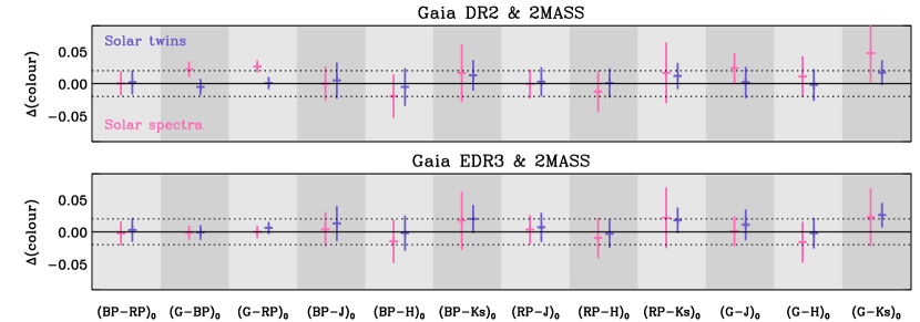
Figure 13: Difference between the colours of the Sun listed in Table 4 and those derived by averaging the colours of four absolutely calibrated solar reference spectra (pink). Error bars are the squared root of the squared sum of the uncertainties reported in Table 4 and of the standard deviation of the colours derived from our four reference spectra. Also shown is the difference between our colours and those inferred from solar twins (blue). Again, error bars are the squared root of the squared sum of the uncertainties in the two dataset. Dotted lines mark $\pm 0.02$ mag to give a better sense of the typical agreement across different colour indices.

 

¹Research School of Astronomy and Astrophysics, The Australian National University, Canberra, ACT 2611, Australia
²ARC Centre of Excellence for All Sky Astrophysics in 3 Dimensions (ASTRO 3D), Australia
³Centre for Astrophysics and Supercomputing, Swinburne University of Technology, Melbourne, VIC 3122, Australia
⁴Centre for Astrophysics, University of Southern Queensland, Toowoomba, QLD 4350, Australia
⁵Max Planck Institute for Astrophysics, Karl-Schwarzschild-Str. 1, D-85748 Garching, Germany
⁶Sydney Institute for Astronomy, School of Physics, A28, The University of Sydney, NSW 2006, Australia
⁷School of Physics, UNSW, Sydney, NSW 2052, Australia
⁸Institute for Advanced Study, Princeton, NJ 08540, USA
⁹Department of Astrophysical Sciences, Princeton University, Princeton, NJ 08544, USA
¹⁰Observatories of the Carnegie Institution of Washington, 813 Santa Barbara Street, Pasadena, CA 91101, USA
¹¹Monash Centre for Astrophysics, Monash University, Australia
¹²School of Physics and Astronomy, Monash University, Australia
¹³Australian Astronomical Optics, Faculty of Science and Engineering, Macquarie University, Macquarie Park, NSW 2113, Australia
¹⁴Macquarie University Research Centre for Astronomy, Astrophysics & Astrophotonics, Sydney, NSW 2109, Australia
¹⁵Istituto Nazionale di Astrofisica, Osservatorio Astronomico di Padova, vicolo dell’Osservatorio 5, 35122, Padova, Italy
¹⁶Faculty of Mathematics and Physics, University of Ljubljana, Jadranska 19, 1000 Ljubljana, Slovenia
¹⁷Department of Astronomy, Stockholm University, AlbaNova University Centre, SE-106 91 Stockholm, Sweden
¹⁸Department of Physics and Astronomy, Macquarie University, Sydney, NSW 2109, Australia

References

- Alonso et al. (1996a) Alonso A., Arribas S., Martinez-Roger C., 1996a, A&AS, 117, 227
- Alonso et al. (1996b) Alonso A., Arribas S., Martinez-Roger C., 1996b, A&A, 313, 873
- Alonso et al. (1999) Alonso A., Arribas S., Martínez-Roger C., 1999, A&AS, 140, 261
- Asplund & García Pérez (2001) Asplund M., García Pérez A. E., 2001, A&A, 372, 601
- Baines et al. (2018) Baines E. K., Armstrong J. T., Schmitt H. R., Zavala R. T., Benson J. A., Hutter D. J., Tycner C., van Belle G. T., 2018, AJ, 155, 30
- Bigot et al. (2011) Bigot L. et al., 2011, A&A, 534, L3
- Blackwell & Shallis (1977) Blackwell D. E., Shallis M. J., 1977, MNRAS, 180, 177
- Blackwell et al. (1979) Blackwell D. E., Shallis M. J., Selby M. J., 1979, MNRAS, 188, 847
- Blackwell et al. (1980) Blackwell D. E., Petford A. D., Shallis M. J., 1980, A&A, 82, 249
- Blackwell et al. (1991) Blackwell D. E., Lynas-Gray A. E., Petford A. D., 1991, A&A, 245, 567
- Böcek Topcu et al. (2020) Böcek Topcu G. et al., 2020, MNRAS, 491, 544
- Boyajian et al. (2012a) Boyajian T. S. et al., 2012a, ApJ, 746, 101
- Boyajian et al. (2012b) Boyajian T. S. et al., 2012b, ApJ, 757, 112
- Buder et al. (2021) Buder S. et al., 2021, MNRAS
- Cardelli et al. (1989) Cardelli J. A., Clayton G. C., Mathis J. S., 1989, ApJ, 345, 245
- Casagrande (2009) Casagrande L., 2009, Mem. Soc. Astron. Italiana, 80, 727
- Casagrande & VandenBerg (2014) Casagrande L., VandenBerg D. A., 2014, MNRAS, 444, 392
- Casagrande & VandenBerg (2018) Casagrande L., VandenBerg D. A., 2018, MNRAS, 479, L102
- Casagrande et al. (2006) Casagrande L., Portinari L., Flynn C., 2006, MNRAS, 373, 13
- Casagrande et al. (2010) Casagrande L., Ramírez I., Meléndez J., Bessell M., Asplund M., 2010, A&A, 512, A54
- Casagrande et al. (2012) Casagrande L., Ramírez I., Meléndez J., Asplund M., 2012, ApJ, 761, 16
- Casagrande et al. (2019) Casagrande L., Wolf C., Mackey A. D., Nordland er T., Yong D., Bessell M., 2019, MNRAS, 482, 2770
- Casagrande et al. (2014) Casagrande L. et al., 2014, MNRAS, 439, 2060
- Castelli & Kurucz (2003) Castelli F., Kurucz R. L., 2003, in N. Piskunov, W.W. Weiss, D.F. Gray, eds, Modelling of Stellar Atmospheres. IAU Symposium, Vol. 210, p. A20
- Choi et al. (2018) Choi J., Dotter A., Conroy C., Ting Y. S., 2018, ApJ, 860, 131
- Code et al. (1976) Code A. D., Bless R. C., Davis J., Brown R. H., 1976, ApJ, 203, 417
- Evans et al. (2018) Evans D. W. et al., 2018, A&A, 616, A4
- Fitzpatrick (1999) Fitzpatrick E. L., 1999, PASP, 111, 63
- Gaia Collaboration et al. (2021) Gaia Collaboration et al., 2021, A&A, 649, A8
- Gallenne et al. (2018) Gallenne A. et al., 2018, A&A, 616, A68
- González Hernández & Bonifacio (2009) González Hernández J. I., Bonifacio P., 2009, A&A, 497, 497
- Green et al. (2019) Green G. M., Schlafly E., Zucker C., Speagle J. S., Finkbeiner D., 2019, ApJ, 887, 93
- Gustafsson et al. (2008) Gustafsson B., Edvardsson B., Eriksson K., Jørgensen U. G., Nordlund Å., Plez B., 2008, A&A, 486, 951
- Huber et al. (2012) Huber D. et al., 2012, ApJ, 760, 32
- Jofré et al. (2018) Jofré P., Heiter U., Tucci Maia M., Soubiran C., Worley C. C., Hawkins K., Blanco-Cuaresma S., Rodrigo C., 2018, Research Notes of the American Astronomical Society, 2, 152
- Karovicova et al. (2020) Karovicova I., White T. R., Nordlander T., Casagrand e L., Ireland M., Huber D., Jofré P., 2020, A&A, 640, A25
- Lachaume et al. (2019) Lachaume R., Rabus M., Jordán A., Brahm R., Boyajian T., von Braun K., Berger J. P., 2019, MNRAS, 484, 2656
- Maestro et al. (2013) Maestro V. et al., 2013, MNRAS, 434, 1321
- Maíz Apellániz & Weiler (2018) Maíz Apellániz J., Weiler M., 2018, A&A, 619, A180
- Meftah et al. (2018) Meftah M. et al., 2018, A&A, 611, A1
- Meléndez et al. (2006) Meléndez J., Dodds-Eden K., Robles J. A., 2006, ApJ, 641, L133
- Meléndez et al. (2009) Meléndez J., Asplund M., Gustafsson B., Yong D., 2009, ApJ, 704, L66
- Mucciarelli & Bellazzini (2020) Mucciarelli A., Bellazzini M., 2020, Research Notes of the American Astronomical Society, 4, 52
- Mucciarelli et al. (2021) Mucciarelli A., Bellazzini M., Massari D., 2021, arXiv e-prints, arXiv:2106.03882
- Nissen (2015) Nissen P. E., 2015, A&A, 579, A52
- Nissen & Gustafsson (2018) Nissen P. E., Gustafsson B., 2018, A&A Rev., 26, 6
- O’Donnell (1994) O’Donnell J. E., 1994, ApJ, 422, 158
- Prša et al. (2016) Prša A. et al., 2016, AJ, 152, 41
- Rains et al. (2020) Rains A. D., Ireland M. J., White T. R., Casagrande L., Karovicova I., 2020, MNRAS, 493, 2377
- Ramírez & Meléndez (2005) Ramírez I., Meléndez J., 2005, ApJ, 626, 465
- Rieke et al. (2008) Rieke G. H. et al., 2008, AJ, 135, 2245
- Riello et al. (2018) Riello M. et al., 2018, A&A, 616, A3
- Riello et al. (2021) Riello M. et al., 2021, A&A, 649, A3
- Schlafly & Finkbeiner (2011) Schlafly E. F., Finkbeiner D. P., 2011, ApJ, 737, 103
- Schlegel et al. (1998) Schlegel D. J., Finkbeiner D. P., Davis M., 1998, ApJ, 500, 525
- Sharma et al. (2018) Sharma S. et al., 2018, MNRAS, 473, 2004
- Sharma et al. (2019) Sharma S. et al., 2019, MNRAS, 490, 5335
- Spina et al. (2018) Spina L. et al., 2018, MNRAS, 474, 2580
- Thuillier et al. (2004) Thuillier G., Floyd L., Woods T. N., Cebula R., Hilsenrath E., Hersé M., Labs D., 2004, Advances in Space Research, 34, 256
- White et al. (2013) White T. R. et al., 2013, MNRAS, 433, 1262
- White et al. (2018) White T. R. et al., 2018, MNRAS, 477, 4403
- Wittenmyer et al. (2018) Wittenmyer R. A. et al., 2018, AJ, 155, 84