YITP-20-143 IPMU20-0113

Chern-Simons Gravity Dual of BCFT

Tadashi Takayanagi^a,b,c and Takahiro Uetoko^a

^aCenter for Gravitational Physics, Yukawa Institute for Theoretical Physics,

Kyoto University, Kyoto 606-8502, Japan

^bInamori Research Institute for Science, Kyoto 600-8411, Japan

^cKavli Institute for the Physics and Mathematics of the Universe (WPI),

University of Tokyo, Chiba 277-8582, Japan

In this paper we provide a Chern-Simons gravity dual of a two dimensional conformal field theory on a manifold with boundaries, so called boundary conformal field theory (BCFT). We determine the correct boundary action on the end of the world brane in the Chern-Simons gauge theory. This reproduces known results of the AdS/BCFT for the Einstein gravity. We also give a prescription of calculating holographic entanglement entropy by employing Wilson lines which extend from the AdS boundary to the end of the world brane. We also discuss a higher spin extension of our formulation.

1 Introduction

The AdS/CFT correspondence [1] has enabled us to connect the dynamics of a $d$ dimensional conformal field theory (CFT) to that of gravity on a $d+1$ dimensional Anti de-Sitter space (AdS) in a surprising way. We can extend the AdS/CFT to the case where a CFT is defined on a manifold with boundaries, called BCFT (boundary conformal field theory) [2], by imposing a Neumann boundary condition on a surface in the bulk (called the end of the world brane) [3, 4, 5]. This formulation has been called the AdS/BCFT construction and has had many applications such as renormalization group flow [6, 7, 8, 9], condensed matter models [10, 11], non-equilibrium physics including quantum entanglement [12, 13, 14, 15, 16, 17, 18], and computational complexity [19, 20, 21]. Refer also to [22, 23] for string theory embeddings of gravity duals of BCFTs and to [24, 25, 26, 27] for implications to novel string theory backgrounds.

In the holographic entanglement entropy [28, 29, 30] for AdS/BCFT, the minimal surface, whose area computes the holographic entanglement entropy, can terminate on the end of the world brane [4, 5]. This leads to the structure so called the Island [31, 32, 33], which has been successfully applied to studies of black hole information [34, 35, 36, 37, 38]. Moreover, limits of AdS/BCFT lead to a series of codimension two holography [37, 39, 40] (see also [41]).

For $d=2$ dimensional BCFTs, a wide variety of AdS/BCFT setups can be studied analytically, while in higher dimensions, analytical examples are highly limited [42, 43]. It is natural to expect that this special feature of $d=2$ stems from the mathematically beautiful fact that we can formulate three dimensional gravity in terms of SL$(2,R)$ Chern-Simons gauge theory [44, 45]. This Chern-Simons formulation has an important advantage that we can generalize the Einstein gravity to higher spin gravity by replacing the gauge group with SL$(n,R)$ [46, 47, 48], which is a door to studying quantum gravity.

Motivated by this, we present a formulation of AdS/BCFT in the Chern-Simons gauge theory description of three dimensional gravity in this paper. For this we will introduce the end of the world-brane in the SL$(2,R)$ Chern-Simons theory and identity its action with correct boundary terms which reproduce the expected results of AdS/BCFT. Next we will consider the holographic entanglement entropy, which provides us with a useful probe of bulk geometry, expressed in terms of quantum information of the dual CFT. In the Chern-Simons description of gravity, including higher spin gravity, the holographic entanglement entropy is remarkably calculated as an expectation value of a certain Wilson loop [49, 50]. See also e.g. [51, 52, 53, 54, 55, 56, 57] for later progresses and [58, 59, 60, 61, 62, 63] for related works including quantum corrections. For higher spin black hole entropy refer to e.g. [64, 65, 66, 67, 68]. We will extend this calculation of holographic entanglement entropy in Chern-Simons gravity to the case where we have the end of the world brane in the three dimensional bulk. We will find that we can view the end of the world brane can be regarded as a sort of ”D-brane” in Chern-Simons gauge theory.

This paper is organized as follows. In section two we briefly review the AdS/BCFT construction and its holographic entanglement entropy for the Einstein gravity. In section three, we present Chern-Simons gravity formulation of AdS/BCFT. In section four, we give the prescription of calculating holographic entanglement entropy in Chern-Simons gravity in the presence of the end of the world-brane. In section five, we summarize our conclusions and discuss future problems. In appendix A, we present our convention of Lie algebras. In appendix B, we present the details of rewriting the Einstein gravity in terms of Chern-Simons gauge theory. In appendix C, we give a brief summary of the geodesic length in AdS₃ for a convenience.

2 A Brief Review of AdS/BCFT

In this section we would like to give a brief summary of a bottom up construction of gravity duals for CFTs on manifolds with boundaries, called the AdS/BCFT [4, 5]. We focus on the $d=2$ case where BCFT is a two dimensional CFT with a boundary and its gravity dual is three dimensional. We can generalize our construction here to a case with multiple boundaries in straightforward way and we will omit this extension below.

2.1 Construction of AdS/BCFT

Consider a BCFT on a two dimensional manifold $M$ with a boundary $\partial M$. The AdS/BCFT argues that its gravity dual is given by a gravity on a three dimensional space $N$ which satisfies

$$\partial N=M\cup Q,\ \ \ s.t.\ \ \ \partial Q=\partial M.$$ (2.1)

Refer to Fig.1 for an illustration. The manifold $M$ coincides with the asymptotically AdS boundary of $N$. The surface $Q$, which surrounds the gravity dual is called the end of the world brane and is a bulk extension of the boundary $\partial M$. The metric on $N$ and the shape of $Q$ are determined by the equation of motions derived from the bulk gravity action

$$I_{\mbox{gravity}}=I_{EH}+I_{GH},$$ (2.2)

where $I_{EH}$ is the Einstein-Hilbert action

$$I_{EH}=\frac{1}{16\pi G_{N}}\int_{N}\sqrt{-g}(R-2\Lambda)~{},$$ (2.3)

and $I_{GH}$ is the Gibbons-Hawking term with the boundary cosmological constant term:

$$I_{GH}=\frac{1}{8\pi G_{N}}\int_{\partial N}\sqrt{-h}(K-T)~{}.$$ (2.4)

Here $g_{\mu\nu}$ and $h_{ij}$ is the metric of $N$ and $Q$. The tensor $K_{ij}$ is the extrinsic curvature of $Q$ and $K=h^{ij}K_{ij}$ is its trace. The extrinsic curvature is defined by the projection on $Q$ of the covariant derivative of the out-going unit vector $n$, normal to the surface $Q$. The constant $T$ can be interpreted as the tension of the brane $Q$.

By varying $I_{EH}$ with respect to the bulk metric $g$, we obtain the Einstein equation as usual. Moreover, by taking the boundary variation with respect to the boundary metric $h$, we obtain

$$\delta(I_{EH}+I_{GH})=\frac{1}{16\pi G}\int_{\partial N}\sqrt{-h}(K_{ij}-(K-T)h_{ij})\delta h^{ij}~{}.$$ (2.5)

By setting this to be vanishing, we obtain a boundary condition which is either the Dirichlet boundary condition

$$\delta h^{ij}=0,$$ (2.6)

or the Neumann one

$$K_{ij}-(K-T)h_{ij}=0~{}.$$ (2.7)

For the AdS boundary $M$, we impose the Dirichlet boundary condition (2.6) as usual. On the other hand, we impose the Neumann boundary condition (2.7) for the boundary $Q$, i.e. the end of the world brane. In this way, the bulk metric $g$ and the profile of the surface $Q$ is determined by solving the bulk Einstein equation together with the mentioned boundary conditions on $M$ and $Q$. This is a short summary of AdS/BCFT construction.

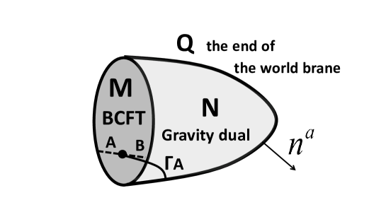
Figure 1: A sketch of AdS/BCFT. We have in mind a $d=2$ example. A BCFT is defined on the manifold $M$ and its gravity dual is given by the region $N$. The boundary of $M$ is extended into the bulk as the surface $Q$, called the end of the world brane. The dotted line represents a time slice on the boundary $M$, which is divided into two subregions $A$ and $B$. The entanglement entropy $S_{A}$ in the BCFT can be holographically computed as the geodesic length of $\Gamma_{A}$ which starts from the boundary $\partial A$ and ends on a point on the surface $Q$, where we minimize the geodesic length by changing the location of the point on $Q$.

2.2 Holographic Entanglement Entropy in AdS/BCFT

The entanglement entropy $S_{A}$ for a subsystem $A$ is defined from a pure quantum state $|\Psi\rangle$ is defined by

$$S_{A}=-\mbox{Tr}[\rho_{A}\log\rho_{A}].$$ (2.8)

We introduced $\rho_{A}$, called the reduced density matrix

$$\rho_{A}=\mbox{Tr}_{B}[|\Psi\rangle\langle\Psi|],$$ (2.9)

where $B$ is the complement of $A$. We can define the entanglement entropy in a BCFT as is so in standard field theories by taking a specific time slice and dividing the time slice into two parts $A$ and $B$. For example, consider a BCFT on a semi-infinite line (times a time direction) which ends on a boundary. If we choose the subsystem $A$ to be a length $l$ interval which extends from the boundary, then the entanglement entropy $S_{A}$ is known to be given by the following formula [69]:

$$S_{A}=\frac{c}{6}\log\frac{l}{\epsilon}+S_{bdy},$$ (2.10)

where $c$ is the central charge of the two dimensional CFT and $\epsilon$ is the UV cut off (i.e. the lattice spacing). The constant term $S_{bdy}$ coincides with an important quantity called the boundary entropy [70], which measures the amount of the degrees of freedom of the boundary.

The holographic dual of the entanglement entropy $S_{A}$ [28, 29, 30] in the AdS/BCFT construction is computed from the following formula [4, 5]:

$$S_{A}=\mbox{Min}\ \mbox{Ext}\left[\frac{\mbox{Area}(\Gamma_{A})}{4G_{N}}\right],\ \ s.t.\ \ \partial\Gamma_{A}=\partial A\cup\partial\Sigma,\ \ \ \Sigma\in Q.$$ (2.11)

where Min and Ext mean that we first extremize the area of $\Gamma_{A}$ and after that we pick up the minimal one among discrete candidates of extremal surface. The crucially new aspect peculiar to the AdS/BCFT, is that the extremal surface $\Gamma_{A}$ can end on the surface $Q$. The region on $Q$ which is surround by $\Gamma_{A}$ is written as $\Sigma$ in (2.11), which is recently called an Island [31, 32, 33]. In our $d=2$ case, $\Gamma_{A}$ is a geodesic which connects $\partial A$ and $Q$, where $\partial\Sigma$ degenerates into a point on $Q$ as depicted in Fig.1. Therefore to calculate the holographic entanglement entropy we need to extremize with respect to the location of a point on $Q$ on which the geodesic $\Gamma_{A}$ ends. This prescription successfully reproduces the expression (2.10) [4, 5] and we will reproduce this in our Chern-Simons gravity formalism later in this paper.

3 Chern-Simons Gravity and Boundary Condition

In this section, we describe a three dimensional Einstein gravity on a manifold with boundaries in terms of Chern-Simons (CS) gravity and determine the boundary condition. We assume a negative cosmological constant. In terms of the CS valuables with $G=SL(2,R)\times SL(2,R)$ we can rewrite $I_{EH}$ (2.3) as [44, 45]

$$I_{EH}=\frac{k}{4\pi}\int_{N}\text{Tr}\left[A\wedge dA+\frac{2}{3}A^{3}\right]-\frac{k}{4\pi}\int_{N}\text{Tr}\left[\bar{A}\wedge d\bar{A}+\frac{2}{3}\bar{A}^{3}\right]+\frac{k}{4\pi}\int_{\partial{N}}\text{Tr}\left[A\wedge\bar{A}\right],$$ (3.1)

where $A$ and $\bar{A}$ can be decomposed into two pairs of connections as

$$A=A^{a}J_{a}=\left(\omega^{a}+e^{a}\right)J_{a},\quad\bar{A}=\bar{A}^{a}J_{a}=\left(\omega^{a}-e^{a}\right)J_{a}.$$ (3.2)

Here $J_{a}\in sl(2,R)$ are explicitly given by

$$J_{1}=\left(\begin{array}[]{cc}0&0\\ -1&0\\ \end{array}\right),\quad J_{0}=\left(\begin{array}[]{cc}1/2&0\\ 0&-1/2\\ \end{array}\right),\quad J_{-1}=\left(\begin{array}[]{cc}0&1\\ 0&0\\ \end{array}\right),$$ (3.9)

and we also define

$$J_{\rho}=J_{0},\ \ \ J_{t}=\frac{J_{1}+J_{-1}}{2},\ \ \ J_{\phi}=\frac{J_{1}-J_{-1}}{2},$$ (3.10)

which obeys

$$[J_{\rho},J_{t}]=-J_{\phi},\ \ \ [J_{t},J_{\phi}]=-J_{\rho},\ \ \ [J_{\phi},J_{\rho}]=J_{t}.$$ (3.11)

We write the three dimensional coordinate $x^{\mu}$ as $(x^{0},x^{1},x^{2})=(t,\phi,\rho)$. Note that $k$ is the CS level with $k=\frac{1}{4G_{N}}$, see also details of this formulation in appendix B.

3.1 Adding Boundary Term

The correct CS gravity action with a boundary $Q$ is given by

$$I_{tot}^{CS}=I_{EH}+I_{GH}$$ (3.12)

with (2.3) and (2.4). $I_{GH}$ is rewritten as

$$I_{GH}=-\frac{k}{2\pi}\int_{Q}P_{ab}e^{a}\wedge\omega^{b}-\frac{k}{2\pi}\int_{Q}\epsilon_{abc}e^{a}\wedge n^{b}dn^{c}-\frac{kT}{4\pi}\int_{Q}\epsilon_{abc}n^{a}e^{b}\wedge e^{c}~{},$$ (3.14)

where $\epsilon_{abc}$ is the epsilon tensor such that $\epsilon_{t\phi\rho}=1$ and $n^{a}$ is a vector with a unit norm $n^{a}n_{a}=1$. $P_{ab}$ is the projector on $Q$ defined as $P_{ab}=\eta_{ab}-n_{a}n_{b}$ with $\eta_{ab}=2\text{Tr}[J_{a}J_{b}]$. Also we simplified $\int_{Q}d\rho\wedge dt$ as $\int_{Q}$. Note here that, at first, we treat $n^{a}$ as a unit vector field on $Q$ and it is regarded as a dynamical field. After we impose the boundary condition we will find that $n^{a}$ is a normal vector of the surface $Q$.

With (3.1) and (3.14), we find the total variation

$$\begin{aligned} \delta I^{CS}_{tot}&=-\frac{k}{2\pi}\int_{Q}\delta e^{a}\wedge(P_{ab}\omega^{b}+\epsilon_{abc}n^{b}dn^{c}-T\epsilon_{abc}n^{b}e^{c})+\frac{k}{2\pi}\int_{Q}n_{a}n_{b}e^{a}\wedge\delta\omega^{b}\\ &\qquad+\frac{k}{4\pi}\int_{Q}\delta n^{a}\left[4\epsilon_{abc}e^{b}dn^{c}+4n_{b}e^{b}\wedge\omega_{a}-T\epsilon_{abc}e^{b}\wedge e^{c}\right],\end{aligned}$$ (3.15)

where we use the relation

$$\epsilon_{abc}n^{b}(de^{c})=(n_{b}e^{b})\wedge\omega^{a}-e^{a}\wedge(n_{b}\omega^{b})$$ (3.16)

with the equation of motion

$$de^{a}-\epsilon^{a}_{bc}\omega^{b}\wedge e^{c}=0.$$ (3.17)

This leads to the following (Neumann) boundary conditions on $Q$:

$$P_{ab}\omega^{b}+\epsilon_{abc}n^{b}dn^{c}-T\epsilon_{abc}n^{b}e^{c}=0~{},$$ (3.18)

$$n_{a}e^{a}=0~{},$$ (3.19)

$$P_{a^{\prime}a}(4\epsilon^{a}_{bc}e^{b}dn^{c}+4n_{b}e^{b}\wedge\omega^{a}-T\epsilon^{a}_{bc}e^{b}\wedge e^{c})=0~{}.$$ (3.20)

The second condition (3.19) says that $n^{a}$ is a normal vector on $Q$ i.e. if we define the normal unit vector on $Q$ by $N_{\mu}$, then the vector $n^{a}$ is defined by

$$n^{a}=e^{a}_{\mu}N^{\mu}.$$ (3.21)

Note also that we acted $P_{a^{\prime}a}$ in the third condition (3.20) to project to the direction orthogonal to $n^{a}$. This is simply because the variation $\delta n^{a}$ is restricted to $n_{a}\delta n^{a}=0$ because $n^{a}n_{a}=1$. The third condition (3.20) is trivially satisfied if we assume (3.19) and remember that $n_{a}dn^{a}=0$. Therefore once we choose $n^{a}$ to be the normal vector on $Q$, we have only to solve the first equation (3.18), which is equivalent to (2.7) as we show in appendix B.

3.2 Gauge Invariance

Let us consider the gauge transformation

$$\delta A=d\chi+[A,\chi],\ \ \ \ \delta\bar{A}=d\bar{\chi}+[\bar{A},\bar{\chi}].$$ (3.22)

If write $\chi=\alpha+\beta$ and $\bar{\chi}=\alpha-\beta$, then the gauge transformation looks like

$$\delta e=d\beta+[\omega,\beta]+[e,\alpha],$$

$$\delta\omega=d\alpha+[\omega,\alpha]+[e,\beta].$$ (3.23)

First consider the variation of Einstein-Hilbert action $I_{EH}$ i.e, (3.1), which looks like

$$\delta I_{EH}=\frac{k}{4\pi}\int_{Q}(\bar{\chi}-\chi)\wedge[dA+d\bar{A}+A\wedge\bar{A}+\bar{A}\wedge A].$$ (3.24)

Therefore we find that this is vanishing if we impose the boundary condition

$$(\chi-\bar{\chi})|_{Q}=0.$$ (3.25)

Thus the part $\alpha$ of the gauge transformation is still active at the boundary.

The remaining term of $I_{GH}$ (3.14) is

$$I_{GH}=-\frac{k}{2\pi}\int_{Q}\epsilon_{abc}e^{a}\wedge n^{b}(dn^{c}+\epsilon^{c}_{pq}\omega^{p}n^{q})-\frac{kT}{4\pi}\int\epsilon_{abc}n^{a}e^{b}\wedge e^{c}.$$ (3.26)

It is clear that this term is invariant under the $\alpha$ gauge transformation (i.e. the local $SL(2,R)$ transformation), which looks like

$$\delta e=[e,\alpha],\ \ \ \delta n=[n,\alpha],\ \ \ \delta\omega=d\alpha+[\omega,\alpha].$$ (3.27)

Indeed, because $[J_{a},J_{b}]=-\epsilon^{c}_{ab}J_{c}$, we find the $\alpha$ gauge transformation leads to

$$\delta(dn-[\omega,n])=[dn-[\omega,n],\alpha].$$ (3.28)

Thus we can regard $dn-[\omega,n]=Dn^{a}J_{a}$ as the covariant derivative [71] where

$$Dn^{a}=dn^{a}+\epsilon^{a}_{pq}\omega^{p}n^{q},$$ (3.29)

which behaves like a vector under the local $SL(2,R)$ transformation in the same way as $e^{a}$ and $n^{a}$.

3.3 Solutions to Boundary Condition

In this paper, we focus on examples constructed from the Poincare AdS₃

$$ds^{2}=e^{2\rho}(-dt^{2}+d\phi^{2})+d\rho^{2}.$$ (3.30)

We write the gauge fields

$$A=e^{\rho}J_{1}dx^{+}+J_{0}d\rho,\quad\bar{A}=-e^{\rho}J_{-1}dx^{-}-J_{0}d\rho,$$ (3.31)

where $x^{\pm}=t\pm\phi$. The connections are

$$\begin{aligned} e&=e^{a}J_{a}=e^{\rho}J_{\rho}+e^{t}J_{t}+e^{\phi}J_{\phi},\\ \omega&=\omega^{a}J_{a}=\omega^{\rho}J_{\rho}+\omega^{t}J_{t}+\omega^{\phi}J_{\phi}\end{aligned}$$ (3.32)

with

$$\begin{aligned} &e^{\rho}=d\rho,\quad e^{t}=e^{\rho}dt,\quad e^{\phi}=e^{\rho}d\phi,\\ &\omega^{\rho}=0,\quad\omega^{t}=e^{\rho}d\phi,\quad\omega^{\phi}=e^{\rho}dt.\end{aligned}$$ (3.33)

Let us consider the boundary surface $Q$ defined by

$$\phi=g(\rho).$$ (3.34)

The normal vector reads

$$n^{\rho}=-\frac{g^{\prime}(\rho)}{\sqrt{g^{\prime}(\rho)^{2}+e^{-2\rho}}},\ \ \ n^{t}=0,\ \ \ n^{\phi}=\frac{e^{-\rho}}{\sqrt{g^{\prime}(\rho)^{2}+e^{-2\rho}}}.$$ (3.35)

Then the boundary condition (3.18) with the ansatz (3.34) gives explicitly the equation for $a=t$, $a=\phi$ and $a=\rho$ as follows:

$$a=t:\ \ \ g^{\prime 3}+2g^{\prime}e^{-2\rho}+g^{\prime\prime}e^{-2\rho}+T(e^{-2\rho}+g^{\prime 2})^{3/2}=0,$$

$$a=\phi:\ \ \ g^{\prime}+T\sqrt{g^{\prime 2}+e^{-2\rho}}=0,$$

$$a=\rho:\ \ \ g^{\prime}+T\sqrt{g^{\prime 2}+e^{-2\rho}}=0.$$ (3.36)

These are simply solved as

$$\phi=g(\rho)=\frac{T}{\sqrt{1-T^{2}}}e^{-\rho}+\mbox{const.}$$ (3.37)

which reproduces the known profile of boundary surface $Q$ in AdS/BCFT [4, 5].

3.4 Comment on Higher Spin Generalization

It is intriguing to extend the above construction to the Chern-Simons description of higher spin gravity, whose CFT duals have been known [72, 73, 74] for a while. We can construct a boundary action on $Q$ in higher spin gravity by replacing the SL($2,R$) indices $a,b,c\cdot\cdot\cdot$ in $I_{GH}$ (3.14), in addition to $I_{EH}$ (3.1), with those for SL($n,R$) with $n=3,4,5,\cdot\cdot\cdot$, maintaining the higher spin gauge invariance (refer to appendix A.2 for SL($3,R)$).

It is straightforward to find solutions which can also be embedded in SL($2,R$) theory like (3.37), by solving the boundary conditions derived from this SL($n,R$) boundary action. However, it turns difficult to find genuine new solutions, which cannot be embedded in SL($2,R$) theory. We believe this is because we did not take into account higher spin charges in the boundary action. We expect we can construct non-trivial solutions peculiar to higher spin gravity if we further add new terms to (3.14) which will make solutions with higher spin charge consistent. This may be regarded as a generalization of the tension term in (3.14) for the SL($2,R$) theory. We would like to leave this as an important future problem.

4 HEE in AdS/BCFT from Wilson Lines

In this section, we extend the calculations of holographic entanglement entropy in higher spin gravity, using Wilson lines pioneered in [49, 50] to our AdS/BCFT setups. The basic idea is that a Wilson line describes a propagation of a massive particle. In AdS/CFT, such a massive particle is dual to a primary operator in a CFT. If we consider a twist operator which appears in the replica computation of entanglement entropy, as a primary operator, then we can read off the holographic entanglement entropy from the expectation value of Wilson line in the higher spin gravity. In our AdS/BCFT, we need to carefully treat the presence of the end of the world brane $Q$, on which the Wilson line ends. We will start our argument with the CS gravity with the gauge group SL($2,R$) and finally we extend it to higher spin gravity with the group SL($3,R$). For explicit calculations in this section, we choose the Poincare AdS₃ (3.30) as a basic example of background. However, it should be straightforward to analyze more general examples in our framework.

Let us first introduce the Wilson line operator [49, 50, 75]

$$W_{R}(C)=\langle U_{f}|P\exp\bigg{(}\int_{C}A\bigg{)}P\exp\bigg{(}\int_{C}\bar{A}\bigg{)}|U_{i}\rangle,$$ (4.1)

where $R$ is a representation of the gauge group $G$, and $C$ is an open path from an initial state $|U_{i}\rangle$ to a final state $|U_{f}\rangle$. Also $P$ means the path ordering. According to [49], the evaluation of Wilson line for a curve $C$ is also given by

$$W_{R}(C)=\int[DU][DP]e^{-I(U,P)_{C}}~{},$$ (4.2)

where $U(s)$ is the world line field on $s\in[s_{i},s_{f}]$ and $P$ is a canonical momentum conjugate to $U$. Here $I(U,P)_{C}$ is the auxiliary system which lives on the Wilson line, and the path integral corresponds to the trace over $R$ in (4.1). In the saddle point approximation, this path integral gives the bulk geodesic length $D_{i,f}$ from $|U_{i}\rangle$ to $|U_{f}\rangle$ as

$$\log W_{R}(C)\propto D_{i,f}.$$ (4.3)

The Wilson line (4.2) depends on only the end point of path $C$ and the representation $R$. Indeed the former gives the length, while the latter contains the character of a massive particle like mass and spin. Thus the bulk conical singularity by the backreaction of Wilson lines is controlled by $R$. The highest weight of $R$ is labeled by the quadratic Casimir $c_{2}$ and indeed we may evaluate the entanglement entropy as

$$S_{EE} =-\log\left(W_{R}(C)\right)=\sqrt{2c_{2}}D_{i,f}$$ (4.4)

with fixing $\sqrt{2c_{2}}\rightarrow c/6$.

4.1 Geodesics between Bulk Two Points

Firstly we give a simple example in Poincare AdS with no additional boundary $Q$. In the case of $G=SL(2,R)\times SL(2,R)$, the evaluation of Wilson line for a curve $C$ is given by the action [49]:

$$I(U,P)_{C}=\int_{C}ds\left(\text{Tr}[PU^{-1}D_{s}U]+\lambda(s)(\text{Tr}[P^{2}]-c_{2})\right),$$ (4.5)

where $U$ and $P$ live in the group manifold $SL(2,R)$ and the Lie algebra $sl(2,R)$, and $D_{s}U=dU/ds+A_{s}U-U\bar{A}_{s}$ with $A_{s}\equiv A_{\mu}dx^{\mu}/ds$. Since the equation of motion for this action leads to

$$U^{-1}D_{s}U+2\lambda P=0,\quad\frac{dP}{ds}=0,\quad\text{Tr}[P^{2}]=c_{2},$$ (4.6)

the on-shell action is evaluated as

$$I(U,P)_{C}|_{on-shell}=-2c_{2}\int_{C}ds\lambda(s).$$ (4.7)

In the paper [49], using this action, it was shown that the Wilson line which connects two points on the AdS boundary $\rho=\rho_{\infty}\to\infty$, correctly reproduces the geodesic length when we impose the Dirichlet boundary condition at the end points. Therefore the holographic entanglement entropy can be computed via a Wilson line. Below in this subsection, as a first step, we will generalize this calculation to the case where the end points of Wilson line are both situated at the bulk AdS.

To begin with, let us consider possibilities of boundary conditions we can impose at the end points of Wilson line. If the curve has an end point, we need to impose

$$\delta I(U,P)_{C}=[PU^{-1}\delta U]=0,$$ (4.8)

at the end point in order to make the variation of the total action $\delta I(U,P)_{C}$ vanishes. This leads to either the Dirichlet boundary condition $\delta U=0$ or the Neumann boundary condition $P=0$.

For the Poincare solution of the Chern–Simons gravity we can write it in the following pure gauge form (3.31):

$$A=LdL^{-1},\quad\bar{A}=R^{-1}dR,$$ (4.9)

where $L$ and $R$ are given by

$$L=P\exp\left(-\int_{(0,0,0)}^{(t,\phi,\rho)}A\right),\quad R=P\exp\left(-\int^{(0,0,0)}_{(t,\phi,\rho)}\bar{A}\right).$$ (4.10)

Let us start with the trivial solution

$$U_{0}(s)=u_{0}e^{-2\alpha(s)P_{0}},$$ (4.11)

where $\lambda=d\alpha/ds$, and indeed the actual solution and momentum are found by the gauge transformation as

$$\begin{aligned} U(s)&=L(s)\cdot U_{0}\cdot R(s),\quad P(s)=R(s)^{-1}\cdot P_{0}\cdot R(s).\end{aligned}$$ (4.12)

Eliminating $u_{0}$ for $U(s_{i})$ and $U(s_{f})$, we obtain

$$\begin{aligned} e^{-2(\alpha(s_{f})-\alpha(s_{i}))P_{0}}=(R(s_{i})U^{-1}(s_{i})L(s_{i}))(R(s_{f})U^{-1}(s_{f})L(s_{f}))^{-1}.\end{aligned}$$ (4.13)

We now impose the Dirichlet boundary condition $\delta U=0$ at both end points. In particular, we choose

$$U(s_{i})=U(s_{f})=1,$$ (4.14)

at both end points. Then we find (refer to (A.12))

$$\begin{aligned} &e^{-2(\alpha(s_{f})-\alpha(s_{i}))P_{0}}\\ &\quad=(R(s_{i})L(s_{i}))(R(s_{f})L(s_{f}))^{-1}\\ &\quad=\left(\begin{array}[]{cc}e^{\rho_{f}-\rho_{i}}+x_{i}^{-}(x_{f}^{+}-x_{i}^{+})e^{\rho_{i}+\rho_{f}}&x_{f}^{-}e^{\rho_{f}-\rho_{i}}-x_{i}^{-}e^{\rho_{i}-\rho_{f}}+x_{i}^{-}x_{f}^{-}(x_{f}^{+}-x_{i}^{+})e^{\rho_{i}+\rho_{f}}\\ (x_{i}^{+}-x_{f}^{+})e^{\rho_{i}+\rho_{f}}&e^{\rho_{i}-\rho_{f}}+x_{f}^{-}(x_{i}^{+}-x_{f}^{+})e^{\rho_{i}+\rho_{f}}\\ \end{array}\right)\end{aligned}$$ (4.15)

with the useful relation

$$\begin{aligned} &e^{\alpha J_{\pm 1}}={\bf 1}+\alpha J_{\pm 1},\\ &e^{\rho J_{0}}=\cosh\frac{\rho}{2}\cdot{\bf 1}+2\sinh\frac{\rho}{2}\cdot J_{0}.\end{aligned}$$ (4.16)

By taking the trace, the LHS of (4.15) becomes

$$\text{Tr}\big{[}e^{-2(\alpha(s_{f})-\alpha(s_{i}))P_{0}}\big{]}=2\cosh\big{(}-\sqrt{2c_{2}}(\alpha(s_{f})-\alpha(s_{i}))\big{)}$$ (4.17)

and the RHS is

$$2\cosh(\rho_{f}-\rho_{i})-(x_{f}^{+}-x_{i}^{+})(x_{f}^{-}-x_{i}^{-})e^{\rho_{i}+\rho_{f}}=\frac{z_{i}^{2}+z_{f}^{2}-(x_{f}^{+}-x_{i}^{+})(x_{f}^{-}-x_{i}^{-})}{z_{i}z_{f}}$$ (4.18)

with $z=e^{-\rho}$. Thus we obtain

$$\cosh\big{(}-\sqrt{2c_{2}}(\alpha(s_{f})-\alpha(s_{i}))\big{)}=\frac{z_{i}^{2}+z_{f}^{2}-(x_{f}^{+}-x_{i}^{+})(x_{f}^{-}-x_{i}^{-})}{2z_{i}z_{f}}.$$ (4.19)

This manifestly shows that the value of $\sqrt{2c_{2}}|\alpha(s_{f})-\alpha(s_{i})|$ coincides with the geodesic length (refer also to the appendix C for a brief summary of geodesic length in AdS₃).

If we choose $s_{i}$ and $s_{f}$ to be at the AdS boundary such that $\rho_{i}=\rho_{f}=\rho_{\infty}\to\infty$, we can evaluate the entanglement entropy in AdS₃ such as

$$S_{EE}=I(U,P)_{C}|_{on-shell}=\frac{c}{3}\log\left(\frac{\sqrt{(\Delta\phi)^{2}-(\Delta t)^{2}}}{\epsilon}\right)$$ (4.20)

where we set $\sqrt{2c_{2}}=c/6$, $\epsilon=e^{-\rho_{\infty}}$, $\Delta t=t_{f}-t_{i}$, and $\Delta\phi=\phi_{f}-\phi_{i}$.

4.2 Holographic Entanglement Entropy in AdS/BCFT from Chern-Simons Gravity

Now we would like to get back to our original problem. We would like to formulate the calculation of holographic entanglement entropy in the presence of the boundary surface $Q$ within our CS gravity formalism. The AdS/BCFT prescription argues that the holographic entanglement entropy when the subsystem A is a half line, is computed from the length of the geodesic which connects a boundary point and a point on $Q$ as we reviewed in section 2.2. Even for generic choices of subsystem $A$ in two dimensional BCFTs, the holographic entanglement entropy is basically given by combining the result in this half line case and the result for a connected geodesic (4.20).

We express the initial point at $s_{i}=s_{0}$ and the final point at $s_{f}=s_{1}$ in AdS₃ (3.30) by the coordinates $(t_{0},\rho_{0},\phi_{0})$ and $(t_{1},\rho_{1},\phi_{1})$, respectively. We take $(t_{0},\rho_{0},\phi_{0})$ to be at the AdS boundary i.e. $\rho_{0}\to\infty$ and take $(t_{1},\rho_{1},\phi_{1})$ to be on the surface $Q$ i.e. $\phi_{1}=\frac{T}{\sqrt{1-T^{2}}}e^{-\rho_{1}}$ in (3.37). Refer to Fig. 2 for a sketch.

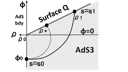
Figure 2: A sketch of a Wilson line which computes the entanglement entropy in AdS/BCFT. The colored region is the physical spacetime for the AdS/BCFT. The dotted curve describes the minimal length one. We omit the time direction. In CS gravity description, for any choices of a point $Q$ the Wilson line takes the same expectation value once we impose our Neumann-Dirichlet boundary condition.

Remember that we can write $U(s)$ as follows

$$U(s)=P\exp\left(-\int^{(t(s),\rho(s),\phi(s))}_{(0,0,0)}A_{\mu}dx^{\mu}\right)\cdot u_{0}e^{-2\alpha(s)P_{0}}\cdot P\exp\left(-\int^{(0,0,0)}_{(t(s),\rho(s),\phi(s))}\bar{A}_{\mu}dx^{\mu}\right),$$

(4.21)

and this allows us to write the variation of the end point $(t(s),\rho(s),\phi(s))$ as

$$\delta U=-(A_{\mu}U-U\bar{A}_{\mu})dx^{\mu}.$$ (4.22)

Let us first count the number of integration constants in the solution (4.21) for the interval $s_{0}\leq s\leq s_{1}$, which should all be fixed after imposing a complete set of boundary conditions. There are totally six integration constants i.e. the $SL(2,R)$ matrix $u_{0}$ (three degrees of freedom) and the traceless matrix $P_{0}$ with the constraint $\mbox{Tr}[P^{2}]=c_{2}$ (two degrees of freedom), and finally the value of $\alpha(s_{1})$. Note that we simply set

$$\alpha(s_{0})=0,$$ (4.23)

because this can be absorbed into $u_{0}$.

First we impose the Dirichlet boundary condition

$$U(s_{0})=1,$$ (4.24)

as we did before for the end points on the AdS boundary. Together with (4.23), this boundary condition (4.24) fixes

$$u_{0}=e^{J_{1}x^{+}_{0}}e^{2J_{0}\rho_{0}}e^{J_{-1}x^{-}_{0}},$$ (4.25)

via the relation (4.21). This determines three out of six constants.

We argue the remaining three boundary conditions are given by a mixed Dirichlet-Neumann boundary condition at $s=s_{1}$, whose detail will be described as follows. First, let us introduce the parameters of SL(2,R) manifold $(\hat{t},\hat{\rho},\hat{\phi})$ and write the constant matrix part of $U(s)$:

$$u_{0}e^{-\alpha(s_{1})P_{0}}\equiv e^{J_{1}\hat{x}^{+}}e^{2J_{0}\hat{\rho}}e^{J_{-1}\hat{x}_{-}}.$$ (4.26)

In other words, we can parameterize the matrix $U(s_{1})$ we are interested in as follows

$$U(s_{1})=e^{-J_{0}\rho_{1}}e^{-J_{1}x^{+}_{1}}\cdot e^{J_{1}\hat{x}^{+}}e^{2J_{0}\hat{\rho}}e^{J_{-1}\hat{x}^{-}}\cdot e^{-J_{-1}x^{-}_{1}}e^{-J_{0}\rho_{1}}.$$ (4.27)

For each value of $(t_{1},\rho_{1},\phi_{1})$, our Dirichlet boundary condition is to require that the point $(\hat{t},\hat{\rho},\hat{\phi})$ is included in the surface $Q$ given by (3.37) i.e.

$$\hat{\phi}=\frac{T}{\sqrt{1-T^{2}}}e^{-\hat{\rho}}.$$ (4.28)

Let us define the codimension one subspace $\Sigma(Q)$ of SL($2,R$) as (refer to Fig.3)

$$\Sigma(Q)=\{e^{J_{1}\hat{x}^{+}}e^{2J_{0}\hat{\rho}}e^{J_{-1}\hat{x}_{-}}\in\mbox{SL($2,R$)}\ |\ (\hat{t},\hat{\rho},\hat{\phi})\in Q\}.$$ (4.29)

This is a group counterpart of the surface $Q$ in the AdS/BCFT. Then our Dirichlet boundary condition is equivalently written as

$$e^{J_{1}x^{+}_{1}}e^{J_{0}\rho_{1}}\cdot U(s_{1})\cdot e^{J_{0}\rho_{1}}e^{J_{-1}x^{-}_{1}}=e^{J_{1}\hat{x}^{+}}e^{2J_{0}\hat{\rho}}e^{J_{-1}\hat{x}_{-}}\in\Sigma(Q).$$ (4.30)

This is a natural condition by considering the behavior of Wilson lines when we embed the boundary surface $Q$ in the target space namely AdS₃=SL($2,R$).

Next we impose the Neumann condition in the direction parallel to the “D-brane” $\Sigma(Q)$. This can be done by remembering that the variation of $\mbox{Tr}[PU^{-1}\delta U]$ should vanish (4.8), where the variation $\delta U$ is given by the variation of (4.27) by shifting the values of $(\hat{t},\hat{\rho},\hat{\phi})$ with the constraint (4.28) satisfied. This is equivalent to the variation in (4.22) along the surface Q. Thus the Neumann boundary condition is found as

$$v^{\mu}\mbox{Tr}[P(U^{-1}A_{\mu}U-\bar{A}_{\mu})]\bigr{|}_{Q}=0,$$ (4.31)

where $v$ is a vector parallel to the surface $Q$ and thus (4.31) is decomposed into two equations on $Q$ defined by the coordinate $(t_{1},\rho_{1},\phi_{1}=\frac{T}{\sqrt{1-T^{2}}}e^{-\rho_{1}})$:

$$\mbox{Tr}[P(U^{-1}A_{t}U-\bar{A}_{t})]=0,$$ (4.32)

$$\mbox{Tr}[P(U^{-1}A_{\rho}U-\bar{A}_{\rho})]-\frac{T}{\sqrt{1-T^{2}}}e^{-\rho_{1}}\cdot\mbox{Tr}[P(U^{-1}A_{\phi}U-\bar{A}_{\phi})]=0.$$ (4.33)

These conditions guarantee that the on-shell action (i.e. the expectation value of Wilson line) is independent from the values of the end point $(t_{1},\rho_{1})$ on $Q$. Indeed these conditions can be obtained from (4.21) by taking variation of $(x^{+}(s_{1}),x^{-}(s_{1}),\rho(s_{1}))$ along the surface $Q$, with $\alpha(s_{1})$ and $P_{0}$ kept fixed.

Now we are in a position to solve the above two Neumann boundary conditions (4.32), (4.33) and one Dirichlet boundary condition (4.30), which totally provide three constraints we wanted. The two Neumann equations (4.32) and (4.33) fix $P_{0}$ as follows

$$P_{0}=\sqrt{\frac{c_{2}}{2}}\frac{1}{\sqrt{e^{-2\rho_{0}}+\phi_{0}^{2}}}\left(\begin{array}[]{cc}-t_{0}&e^{-2\rho_{0}}+\phi_{0}^{2}-t_{0}^{2}\\ 1&t_{0}\\ \end{array}\right),$$ (4.36)

where this is independent of $t_{1}$ and $\rho_{1}$.

Finally we would like to solve the Dirichlet boundary condition, which should fix $\alpha(s_{1})$. Before that let us note that interestingly, we can show by using (4.25) and (4.36) that (4.26) is equivalent to

$$\hat{t}=t_{0},\ \ \ \ \phi_{0}^{2}+e^{-2\rho_{0}}=\hat{\phi}^{2}+e^{-2\hat{\rho}},$$ (4.37)

which shows that $(\hat{t},\hat{\rho},\hat{\phi})$ is on the geodesic which connects two boundary points $(t_{0},\rho_{0},\phi_{0})$ and $(t_{0},\rho_{0},-\phi_{0})$. Then, our Dirichlet boundary condition, which requires that the point $(\hat{t},\hat{\rho},\hat{\phi})$ is on the surface $Q$ i.e. $\hat{\phi}=\frac{T}{\sqrt{1-T^{2}}}e^{-\hat{\rho}}$, fixes the value of $(\hat{t},\hat{\rho},\hat{\phi})$ to be $(t_{*},\rho_{*},\phi_{*})$ given by

$$t_{*}=t_{0},\ \ \ \ \ e^{-\rho_{*}}=\sqrt{(1-T^{2})(e^{-2\rho_{0}}+\phi_{0}^{2})},\ \ \ \ \ \phi_{*}=T\sqrt{e^{-2\rho_{0}}+\phi_{0}^{2}}.$$ (4.38)

This point $(t_{*},\rho_{*},\phi_{*})$ actually coincides with the special point on $Q$ which has the minimal distance to the boundary point $(t_{0},\rho_{0},\phi_{0})$ among all points on $Q$ on the time slice $t=t_{0}$ (refer to Fig.2). This is the essential reason why this prescription of calculation the holographic entanglement entropy via the Wilson line, matches with the standard one in Einstein gravity reviewed in section 2.2.

After imposing all these conditions, the matrix $U(s_{1})$ is completely fixed as follows:

$$U(s_{1})=e^{-J_{0}\rho_{1}}e^{-J_{1}x^{+}_{1}}\cdot e^{J_{1}x^{+}_{*}}e^{2J_{0}\rho_{*}}e^{J_{-1}x^{-}_{*}}\cdot e^{-J_{-1}x^{-}_{1}}e^{-J_{0}\rho_{1}}.$$ (4.39)

It is important to notice that when $(t_{1},\rho_{1},\phi_{1})=(t_{*},\rho_{*},\phi_{*})$, we find $U(s_{1})=1$. This corresponds to the point on the surface $Q$ which minimize the length of the geodesic.

At the same time, the equation (4.26) fixes the value of $\alpha(s_{1})$ to be

$$e^{\sqrt{2c_{2}}\alpha(s_{1})}=(\sqrt{1+\phi_{0}^{2}e^{2\rho_{0}}}-\phi_{0}e^{\rho_{0}})\cdot\sqrt{\frac{1+T}{1-T}},$$ (4.40)

which leads to the correct geodesic length and the HEE in the limit $\rho_{0}\to\infty$ (assume $\phi_{0}<0$):

$$S_{A}=\frac{c}{6}\log\left(2|\phi_{0}|e^{\rho_{0}}\right)+\frac{c}{6}\log\sqrt{\frac{1+T}{1-T}}.$$ (4.41)

This perfectly reproduces the known expression (2.10) by setting $\epsilon=e^{-\rho_{0}}$. The boundary entropy is given by

$$S_{bdy}=\frac{c}{6}\log\sqrt{\frac{1+T}{1-T}},$$ (4.42)

which agrees with the result in [4, 5].

In this way, we obtain the correct prescription of holographic entanglement entropy for AdS/BCFT via Wilson lines in the CS gravity, such that the results agree with the earlier prescription [4, 5] in Einstein gravity. In the usual AdS/BCFT for Einstein gravity, it is given by the length of geodesic which departs from the AdS boundary and ends on the surface $Q$ and we minimize the length by changing the location of endpoint on $Q$. In our new calculation in CS gravity, we consider a trajectory of $U(s)$ from the boundary point $s=s_{0}$ to the surface $\Sigma_{Q}$ in the SL(2,R) group manifold. Note that the result does not depend on the end point of the Wilson line, as opposed to the standard holographic entanglement entropy for Einstein gravity. In our CS calculation, the end of the world brane $Q$ looks like a ”D-brane” for a particle moving in the SL($2,R$) group manifold as in Fig.3.

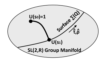
Figure 3: A sketch of computation of holographic entanglement entropy from the view point of SL(2,R) group manifold. A trajectory of $U(s)$ in the SL(2,R) group manifold is depicted as a thick curve with dots at its ends. We impose the initial condition $U(s_{0})=1$ and the Dirichlet-Neumann boundary condition such that $U(s_{1})$ is on $\Sigma_{Q}$, which is a codimension one subspace of SL(2,R).

4.3 Comments on Extension to Higher Spin Gravity

It is intriguing to extend the above prescription of computing holographic entanglement entropy to that for higher spin gravity. In the case of $G=SL(3,R)\times SL(3,R)$, the evaluation of Wilson line is also given by the action [49]

$$I(U,P)_{C}=\int_{C}ds\left(\text{Tr}[PU^{-1}D_{s}U]+\lambda_{2}(s)(\text{Tr}[P^{2}]-c_{2})+\lambda_{3}(s)(\text{Tr}[P^{3}]-c_{3})\right),$$ (4.43)

where we define $\text{Tr}[P^{2}]\equiv P^{a}P^{b}\delta_{ab}$ and $\text{Tr}[P^{3}]\equiv P^{a}P^{b}P^{c}t_{abc}$, see appendix A.2 for details. To evaluate (4.43), we use the equation of motion

$$D_{s}P=0,\quad U^{-1}D_{s}U+2\lambda_{2}(s)P+3\lambda_{3}(s)P\times P=0,\quad\text{Tr}[P^{2}]=c_{2},\quad\text{Tr}[P^{3}]=c_{3}$$ (4.44)

with the definition

$$P\times P=t_{abc}T^{a}P^{b}P^{c}.$$ (4.45)

The on-sell action becomes

$$\begin{aligned} I(U,P)_{C}|_{on-shell}&=-\int_{C}ds(2c_{2}\lambda_{2}(s)+3c_{3}\lambda_{3}(s)).\end{aligned}$$ (4.46)

Note here that we demand $c_{3}=0$ for the purpose of computing entanglement entropy. If we consider the case of $c_{3}\neq 0$, we should give the different interpretation for expectation value of Wilson lines instead of the entanglement entropy in the dual CFTs.

We also start with the trivial solution

$$U_{0}=u_{0}e^{-2\alpha_{2}(s)P_{0}-3\alpha_{3}(s)(P_{0}\times P_{0})}.$$ (4.47)

As in section 4.1, we find that the evaluated on-shell action is given by

$$\begin{aligned} I(U,P)_{C}|_{on-shell}&=-2c_{2}\Delta\alpha_{2}-3c_{3}\Delta\alpha_{3},\end{aligned}$$ (4.48)

and obtain the relation

$$\begin{aligned} e^{-2\Delta\alpha_{2}P_{0}-3\Delta\alpha_{3}(P_{0}\times P_{0})}&=(R(s_{i})U^{-1}(s_{i})L(s_{i}))(R(s_{f})U^{-1}(s_{f})L(s_{f}))^{-1},\end{aligned}$$ (4.49)

with $\Delta\alpha_{N}=\alpha_{N}(s_{f})-\alpha_{N}(s_{i})$. Using the above two equations, we find

$$\begin{aligned} S_{EE}=I(U,P)_{C}|_{on-shell}=\text{Tr}\left[P_{0}\log\Big{(}(R(s_{i})U^{-1}(s_{i})L(s_{i}))(R(s_{f})U^{-1}(s_{f})L(s_{f}))^{-1}\Big{)}\right],\end{aligned}$$ (4.50)

which is the general expression for $G=SL(N,R)\times SL(N,R)$ since this is independent of $G$, see also [75].

Let us next consider the case with the boundary surface $Q$. According to the section 4.2, the boundary condition for $U(s)$ is given by (using (4.39))

$$U(s_{0})=1,\quad U(s_{1})=e^{-J_{0}\rho_{1}}e^{-J_{1}x^{+}_{1}}\cdot e^{J_{1}x^{+}_{*}}e^{2J_{0}\rho_{*}}e^{J_{-1}x^{-}_{*}}\cdot e^{-J_{-1}x^{-}_{1}}e^{-J_{0}\rho_{1}},$$ (4.51)

where $(\rho_{*},x^{\pm}_{*})$ are given by the same values (4.38). Note that this again follows from the Dirichlet-Neumann boundary condition (4.30), which is embedded into SL($2,R$) in an obvious way. Thus we obtain the following result for AdS/BCFT in higher spin gravity:

$$\begin{aligned} S_{EE}=\text{Tr}\left[P_{0}\log\Big{(}(R(s_{0})L(s_{0}))(R(s_{*})L(s_{*}))^{-1}\Big{)}\right]\end{aligned}$$ (4.52)

which reproduce the proper geodesic length and reduces to (4.41) for $N=2$.

Since the precise boundary action in CS formalism is not available at present, we do not know what profiles of the end of the world brane are allowed in the presence of higher spin fields. Therefore the above analysis is limited to the case where we can embed the solution to the subgroup SL($2,R$). Nevertheless, we may expect to obtain the boundary condition we need to impose for Wilson lines by a straightforward generalization of the “D-brane condition” (4.30) from SL($2,R$) to SL($n,R$). We would like to leave a full analysis of holographic entanglement entropy for higher spin gravity for an important future problem.

5 Conclusion and Discussion

In this paper, we presented a formulation of three dimensional AdS/BCFT in terms of Chern-Simons (CS) gravity. In the first half part, we gave the correct boundary action of CS gravity which precisely reproduces the AdS/BCFT in Einstein gravity. For this we introduce a dynamical vector on the end of the world brane $Q$ and impose boundary conditions by varying the total action including the boundary terms. In the later half part, we presented the prescription of computing the holographic entanglement entropy in our CS gauge theoretic description of AdS/BCFT. By employing the Wilson line calculations, the holographic entanglement entropy $S_{A}$ for a subsystem $A$ can be obtained from a Wilson line which connects the AdS boundary point and a point on the end of the world brane $Q$. The former coincides with the point $\partial A$ as usual and the latter can be an arbitrary point on $Q$. The most non-trivial ingredient is the boundary condition at the point on $Q$ for the Wilson line calculation. We argue that this boundary condition is given by a mixed Neumann-Dirichlet boundary condition, where the end of the world brane $Q$ looks like a “D-brane” in the SL($2,R$) group manifold, if we think the Wilson line is analogous to an open string. We also confirmed that our prescription in CS gravity correctly reproduces the know result in BCFTs. Moreover, we gave an extension of our prescription of holographic entanglement entropy to that for higher spin gravity in a simple example.

We expect our results in this paper provide an important first step when we try to fully generalize the AdS/BCFT in higher spin gravity, where the boundary surface $Q$ can have higher spin charges. For example, our boundary action (3.14) and our Neumann-Dirichlet boundary condition: (4.32), (4.33) and (4.30), at a point on $Q$ for the Wilson line computation, have a straightforward generalization from the SL($2,R$) to SL($n,R$) group. Even though we might expect some additional ingredients, these will provide useful clues to formulate the AdS/BCFT for higher spin gravity. A non-trivial test of correctness of holographic entanglement entropy in higher spin gravity will be the strong subadditivity (SSA). This is because in the Wilson line formalism, the derivation of SSA looks difficult as there is no minimization procedure involved, while in the standard holographic entanglement entropy, the proof of SSA follows directly from the minimal surface property [76, 77]. We would like to come back to these important problems in our future publication.

Acknowledgements

We would like to thank Yasuaki Hikida for various discussions. TT is supported by the Simons Foundation through the “It from Qubit” collaboration. TT is supported by Inamori Research Institute for Science and World Premier International Research Center Initiative (WPI Initiative) from the Japan Ministry of Education, Culture, Sports, Science and Technology (MEXT). TT is supported by JSPS Grant-in-Aid for Scientific Research (A) No. 16H02182 and by JSPS Grant-in-Aid for Challenging Research (Exploratory) 18K18766. TU is supported by the Grant-in-Aid for JSPS Research Fellow, No.19J11212.

Appendix A Lie Algebra

A.1 $sl(2)$ Conventions

We denote the generators of $sl(2,R)$ as $J_{a}$, which satisfy

$$[J_{a},J_{b}]=\epsilon_{abc}J^{c}.$$ (A.1)

In the case of the fundamental representation of $sl(2)$, the generators are written as

$$J_{1}=\left(\begin{array}[]{cc}0&0\\ -1&0\\ \end{array}\right),\quad J_{0}=\left(\begin{array}[]{cc}1/2&0\\ 0&-1/2\\ \end{array}\right),\quad J_{-1}=\left(\begin{array}[]{cc}0&1\\ 0&0\\ \end{array}\right).$$ (A.8)

The metric is defined as

$$\eta_{ab}=2\text{Tr}[J_{a}J_{b}].$$ (A.9)

In our calculations of this paper, the following identity is useful:

$$e^{J_{-1}\alpha}e^{-2\rho J_{0}}e^{-J_{1}\beta}e^{2\eta J_{0}}e^{-J_{-1}\gamma}=\left(\begin{array}[]{cc}e^{\eta-\rho}+e^{\eta+\rho}\alpha\beta&e^{-\eta+\rho}\alpha-e^{\eta-\rho}\gamma-e^{\eta+\rho}\alpha\beta\gamma\\ e^{\eta+\rho}\beta&e^{-\eta+\rho}-e^{\eta+\rho}\beta\gamma\\ \end{array}\right).$$ (A.12)

A.2 $sl(3)$ Conventions

We also denote the generators of $sl(3)$ as $T_{a}=\{L_{i},W_{m}\}$ with $i=-1,0,1$ and $m=-2,\dots,2$, which satisfies

$$\begin{aligned} &[L_{i},L_{j}]=(i-j)L_{i+j},\\ &[L_{i},W_{m}]=(2i-m)W_{i+m},\\ &[W_{m},W_{n}]=-\frac{1}{3}(m-n)(2m^{2}+2n^{2}-mn-8).\end{aligned}$$ (A.13)

In the case of fundamental representation of $sl(3)$, the generators are written as

$$\begin{aligned} L_{1}&=\left(\begin{array}[]{ccc}0&0&0\\ 1&0&0\\ 0&1&0\\ \end{array}\right),\quad L_{0}=\left(\begin{array}[]{ccc}1&0&0\\ 0&0&0\\ 0&0&-1\\ \end{array}\right),\quad L_{-1}=\left(\begin{array}[]{ccc}0&-2&0\\ 0&0&-2\\ 0&0&0\\ \end{array}\right),\\ W_{2}&=\left(\begin{array}[]{ccc}0&0&0\\ 0&0&0\\ 2&0&0\\ \end{array}\right),\quad W_{1}=\left(\begin{array}[]{ccc}0&0&0\\ 1&0&0\\ 0&-1&0\\ \end{array}\right),\quad W_{0}=\frac{2}{3}\left(\begin{array}[]{ccc}1&0&0\\ 0&-2&0\\ 0&0&1\\ \end{array}\right),\\ W_{-1}&=\left(\begin{array}[]{ccc}0&-2&0\\ 0&0&2\\ 0&0&0\\ \end{array}\right),\quad W_{-2}=\left(\begin{array}[]{ccc}0&0&8\\ 0&0&0\\ 0&0&0\\ \end{array}\right).\end{aligned}$$ (A.14)

The symmetric tensors are defined as

$$\delta_{ab}=\frac{1}{2}\text{Tr}[T_{a}T_{b}],\quad h_{abc}=\text{Tr}[T_{(a}T_{b}T_{c)}].$$ (A.15)

Appendix B Chern–Simons Formulation of Einstein Gravity

As (2.3) and (2.4), the three dimensional gravity on $\mathcal{M}$ is written by the metric formulation:

$$\begin{aligned} I_{tot}&=I_{EH}+I_{GH},\\ &=\frac{1}{16\pi G}\int_{\mathcal{M}}d^{3}x\sqrt{-g}(R-2\Lambda)+\frac{1}{8\pi G}\int_{\partial\mathcal{M}}d^{2}x\sqrt{-g}K.\end{aligned}$$ (B.1)

Here the Gibbons–Hawking term $I_{GH}$ needs to be added in order to make the variation principle sensible since the variation of $I_{EH}$ contains $\delta\partial_{\rho}g_{ij}$ and this term spoils a variational principle on $\partial\mathcal{M}$. Thus we find

$$\delta I_{tot}=\frac{1}{16\pi G}\int_{M}\sqrt{-g}(K_{ij}-Kg_{ij})\delta g^{ij},$$ (B.2)

and it leads to the two types of conditions

$$\begin{aligned} &\mbox{Dirichlet}:~{}\delta g^{ij}=0,\\ &\mbox{Neumann}:~{}K_{ij}-Kg_{ij}=0.\end{aligned}$$ (B.3)

Note here that we chose the following coordinate system

$$ds^{2}=g_{\mu\nu}dx^{\mu}dx^{\nu}=d\rho^{2}+g_{ij}dx^{i}dx^{j}.$$ (B.4)

B.1 Vielbein Formalism

We may translate from the metric formalism to the vielbein formalism with the basic variables, which consists of vielbeins $e^{a}_{\mu}$ and spin connections $\omega^{a}_{\mu b}$. The metric $g_{\mu\nu}$ is written in terms of vielbeins as

$$g_{\mu\nu}=e^{a}_{\mu}e^{b}_{\nu}\eta_{ab},$$ (B.5)

and covariant derivative of $V^{a}=V^{\mu}e^{a}_{\mu}$ and $V^{a}_{b}=V^{\mu}_{\nu}e^{a}_{\mu}e^{\nu}_{b}$ would be

$$\begin{aligned} &\nabla_{\mu}V^{a}=\partial_{\mu}V^{a}+\omega^{a}_{\mu b}V^{b},\\ &\nabla_{\mu}V^{a}_{b}=\partial_{\mu}V^{a}_{b}+\omega^{a}_{\mu c}V^{c}_{b}-\omega^{c}_{\mu b}V^{a}_{c}.\end{aligned}$$ (B.6)

Then, the Riemann tensor can be written in terms of the spin connections as

$$R=d\omega+\omega\wedge\omega,$$ (B.7)

or alternatively $R^{a}_{\mu\nu b}=\partial_{\mu}\omega^{a}_{\nu b}-\partial_{\nu}\omega^{a}_{\mu b}+[\omega_{\mu},\omega_{\nu}]^{a}_{b}$.

With above setups, the Einstein-Hilbert action is written as

$$\begin{aligned} I_{EH}&=\frac{1}{16\pi G}\int_{\mathcal{M}}\epsilon_{abc}e^{a}\wedge\left(R^{bc}-\frac{\Lambda}{3}e^{b}\wedge e^{c}\right)\\ &=\frac{1}{16\pi G}\int_{\mathcal{M}}\left[e^{a}\wedge\left(2d\omega_{a}+\epsilon_{abc}\omega^{b}\wedge\omega^{c}\right)-\frac{\Lambda}{3}\epsilon_{abc}e^{a}\wedge e^{b}\wedge e^{c}\right],\end{aligned}$$ (B.8)

where we use the relation

$$d^{3}x =\frac{1}{3!}\epsilon_{\mu\nu\sigma}dx^{\mu}\wedge dx^{\nu}\wedge dx^{\sigma},$$ (B.9)

$$\sqrt{-g} =|e|=-\frac{1}{3!}\epsilon_{abc}\epsilon^{\mu\nu\sigma}e^{a}_{\mu}e^{b}_{\nu}e^{c}_{\sigma},$$ (B.10)

$$R^{ab} =d\omega^{ab}+\omega^{a}_{c}\wedge\omega^{cb},$$ (B.11)

$$\omega^{a} =\frac{1}{2}\epsilon^{abc}\omega_{bc}.$$ (B.12)

The the Gibbons–Hawking term is also rewritten

$$\begin{aligned} I_{GH}=-\frac{1}{8\pi G}\int_{\partial\mathcal{M}}P_{ab}e^{a}\wedge\omega^{b}-\frac{1}{8\pi G}\int_{\partial\mathcal{M}}\epsilon_{abc}e^{a}\wedge n^{b}dn^{c}.\end{aligned}$$ (B.13)

Here we use the following relations

$$K =e^{i}_{a}(\partial_{i}n^{a}+\epsilon^{a}_{~{}cb}\omega_{i}^{c}n^{b}),$$ (B.14)

$$d^{2}x =\frac{1}{2}\epsilon_{ij}dx^{i}\wedge dx^{j},$$ (B.15)

$$\sqrt{-g} =\frac{1}{2}\epsilon_{abc}\epsilon^{ij}e^{a}_{i}e^{b}_{j}n^{c},$$ (B.16)

and find

$$\begin{aligned} d^{2}x\sqrt{-g}K=-\epsilon_{abc}e^{a}\wedge\left(n^{b}\epsilon^{c}_{~{}de}\omega^{d}n^{e}+n^{b}dn^{c}\right).\end{aligned}$$ (B.17)

Thus the variation of $I_{tot}$ leads to the condition (3.18), (3.19) and (3.20) with $T=0$.

B.2 Chern–Simons Formalism

The Chern–Simons action with the boundary given in (3.1) and (3.14) is obtained from (B.8) as

$$\begin{aligned} I_{EH}=&\frac{k}{4\pi}\int_{\mathcal{M}}\text{Tr}\left[A\wedge dA+\frac{2}{3}A\wedge A\wedge A\right]-\frac{k}{4\pi}\int_{\mathcal{M}}\text{Tr}\left[\bar{A}\wedge d\bar{A}+\frac{2}{3}\bar{A}\wedge\bar{A}\wedge\bar{A}\right]\\ &\qquad+\frac{k}{4\pi}\int_{\partial\mathcal{M}}\text{Tr}\left[A\wedge\bar{A}\right]\end{aligned}$$ (B.18)

with $k=1/(4G)$, $A=A^{a}J_{a}$ and

$$\text{Tr}\left[J_{a}J_{b}\right]=\frac{1}{2}\delta_{ab},\quad\text{Tr}\left[J_{a}J_{b}J_{c}\right]=\frac{1}{4}\epsilon_{abc}.$$ (B.19)

Here we use the relation

$$A^{a}\wedge dA_{a}-\bar{A}^{a}\wedge d\bar{A}_{a}=\frac{2}{\ell}\left(\omega^{a}\wedge de_{a}+e^{a}\wedge d\omega_{a}\right)$$ (B.20)

$$d(A^{a}\wedge\bar{A}_{a})=dA^{a}\wedge\bar{A}_{a}-A^{a}\wedge d\bar{A}_{a}=\frac{2}{\ell}\left(-\omega^{a}\wedge de_{a}+e^{a}\wedge d\omega_{a}\right).$$ (B.21)

Thus the first term of (B.8) is

$$e^{a}\wedge d\omega_{a}=\frac{1}{4}\left(A^{a}\wedge dA_{a}-\bar{A}^{a}\wedge d\bar{A}_{a}+d(A^{a}\wedge\bar{A}_{a})\right),$$ (B.22)

and the second and third ones are

$$\epsilon_{abc}e^{a}\wedge\left(\omega^{b}\wedge\omega^{c}+\frac{1}{3}e^{b}\wedge e^{c}\right)=\frac{\epsilon_{abc}}{6}\left(A^{a}\wedge A^{b}\wedge A^{c}-\bar{A}^{a}\wedge\bar{A}^{b}\wedge\bar{A}^{c}\right).$$ (B.23)

The Gibbons–Hawking term is also rewritten

$$\begin{aligned} I_{GH}=-\frac{k}{2\pi}\int_{\partial\mathcal{M}}\text{Tr}\left[A\wedge\bar{A}\right]+\frac{1}{8\pi G}\int_{\partial\mathcal{M}}e^{a}\wedge n^{b}\left(n_{a}\omega_{b}-\epsilon_{abc}dn^{c}\right),\end{aligned}$$ (B.24)

where we use the relation

$$\begin{aligned} P_{ab}e^{a}\wedge\omega^{b}=e^{a}\wedge\omega_{a}-e^{a}n_{a}\wedge\omega_{b}n^{b}.\end{aligned}$$ (B.25)

Thus the variation of $I_{tot}$ leads to the condition

$$\begin{aligned} &\mbox{Dirichlet}:~{}\delta(A^{a}-\bar{A}^{a})=0,\end{aligned}$$ (B.26)

and (3.18) with $T=0$.

Appendix C Geodesic Length

Consider the metric of global AdS₃

$$ds^{2}=-\cosh^{2}\rho d\tau^{2}+d\rho^{2}+\sinh^{2}\rho d\theta^{2},$$ (C.1)

and Poincare AdS₃:

$$ds^{2}=\frac{dz^{2}-dt^{2}+d\phi^{2}}{z^{2}}.$$ (C.2)

The geodesic length $D$ between two bulk points $(\rho_{1},\tau_{1},\theta_{1})$ and $(\rho_{2},\tau_{2},\theta_{2})$ in the global AdS₃ is given by

$$\cosh D=\cosh\rho_{1}\cosh\rho_{2}\cos(\tau_{1}-\tau_{2})-\sinh\rho_{1}\sinh\rho_{2}\cos(\theta_{1}-\theta_{2}).$$ (C.3)

In the same way the geodesic distance $D=\cosh\sigma$ between two bulk points $(z_{1},\phi_{1},t_{1})$ and $(z_{2},\phi_{2},t_{2})$ in the Poincare AdS₃ is found as

$$\cosh D=\frac{z_{1}^{2}+z_{2}^{2}+(\phi_{1}-\phi_{2})^{2}-(t_{1}-t_{2})^{2}}{2z_{1}z_{2}}.$$ (C.4)

References

- [1] J. M. Maldacena, The Large N limit of superconformal field theories and supergravity, Int. J. Theor. Phys. 38 (1999) 1113 [hep-th/9711200].
- [2] J. L. Cardy, Boundary conformal field theory, hep-th/0411189.
- [3] A. Karch and L. Randall, Open and closed string interpretation of SUSY CFT’s on branes with boundaries, JHEP 06 (2001) 063 [hep-th/0105132].
- [4] T. Takayanagi, Holographic Dual of BCFT, Phys. Rev. Lett. 107 (2011) 101602 [1105.5165].
- [5] M. Fujita, T. Takayanagi and E. Tonni, Aspects of AdS/Bcft, JHEP 11 (2011) 043 [1108.5152].
- [6] M. Gutperle and J. Samani, Holographic RG-flows and Boundary CFTs, Phys. Rev. D 86 (2012) 106007 [1207.7325].
- [7] J. Estes, K. Jensen, A. O’Bannon, E. Tsatis and T. Wrase, On Holographic Defect Entropy, JHEP 05 (2014) 084 [1403.6475].
- [8] N. Kobayashi, T. Nishioka, Y. Sato and K. Watanabe, Towards a -theorem in defect CFT, JHEP 01 (2019) 039 [1810.06995].
- [9] Y. Sato, Boundary entropy under ambient RG flow in the AdS/BCFT model, Phys. Rev. D 101 (2020) 126004 [2004.04929].
- [10] M. Fujita, M. Kaminski and A. Karch, SL(2,Z) Action on AdS/BCFT and Hall Conductivities, JHEP 07 (2012) 150 [1204.0012].
- [11] J. Erdmenger, M. Flory, C. Hoyos, M.-N. Newrzella, A. O’Bannon and J. Wu, Holographic impurities and Kondo effect, Fortsch. Phys. 64 (2016) 322 [1511.09362].
- [12] T. Ugajin, Two dimensional quantum quenches and holography, 1311.2562.
- [13] D. Seminara, J. Sisti and E. Tonni, Corner contributions to holographic entanglement entropy in AdS4/BCFT3, JHEP 11 (2017) 076 [1708.05080].
- [14] D. Seminara, J. Sisti and E. Tonni, Holographic entanglement entropy in AdS4/BCFT3 and the Willmore functional, JHEP 08 (2018) 164 [1805.11551].
- [15] Y. Hikida, Y. Kusuki and T. Takayanagi, Eigenstate thermalization hypothesis and modular invariance of two-dimensional conformal field theories, Phys. Rev. D 98 (2018) 026003 [1804.09658].
- [16] T. Shimaji, T. Takayanagi and Z. Wei, Holographic Quantum Circuits from Splitting/Joining Local Quenches, JHEP 03 (2019) 165 [1812.01176].
- [17] P. Caputa, T. Numasawa, T. Shimaji, T. Takayanagi and Z. Wei, Double Local Quenches in 2D CFTs and Gravitational Force, JHEP 09 (2019) 018 [1905.08265].
- [18] M. Mezei and J. Virrueta, Exploring the Membrane Theory of Entanglement Dynamics, JHEP 02 (2020) 013 [1912.11024].
- [19] S. Chapman, D. Ge and G. Policastro, Holographic Complexity for Defects Distinguishes Action from Volume, JHEP 05 (2019) 049 [1811.12549].
- [20] Y. Sato and K. Watanabe, Does Boundary Distinguish Complexities?, JHEP 11 (2019) 132 [1908.11094].
- [21] P. Braccia, A. L. Cotrone and E. Tonni, Complexity in the presence of a boundary, JHEP 02 (2020) 051 [1910.03489].
- [22] M. Chiodaroli, E. D’Hoker, Y. Guo and M. Gutperle, Exact half-BPS string-junction solutions in six-dimensional supergravity, JHEP 12 (2011) 086 [1107.1722].
- [23] M. Chiodaroli, E. D’Hoker and M. Gutperle, Holographic duals of Boundary CFTs, JHEP 07 (2012) 177 [1205.5303].
- [24] A. Karch and L. Randall, Geometries with mismatched branes, JHEP 09 (2020) 166 [2006.10061].
- [25] C. Bachas, S. Chapman, D. Ge and G. Policastro, Energy Reflection and Transmission at 2D Holographic Interfaces, 2006.11333.
- [26] P. Simidzija and M. Van Raamsdonk, Holo-ween, 6, 2020, 2006.13943.
- [27] H. Ooguri and T. Takayanagi, Cobordism Conjecture in AdS, 2006.13953.
- [28] S. Ryu and T. Takayanagi, Holographic derivation of entanglement entropy from AdS/CFT, Phys. Rev. Lett. 96 (2006) 181602 [hep-th/0603001].
- [29] S. Ryu and T. Takayanagi, Aspects of Holographic Entanglement Entropy, JHEP 08 (2006) 045 [hep-th/0605073].
- [30] V. E. Hubeny, M. Rangamani and T. Takayanagi, A Covariant holographic entanglement entropy proposal, JHEP 07 (2007) 062 [0705.0016].
- [31] G. Penington, Entanglement Wedge Reconstruction and the Information Paradox, JHEP 09 (2020) 002 [1905.08255].
- [32] A. Almheiri, N. Engelhardt, D. Marolf and H. Maxfield, The entropy of bulk quantum fields and the entanglement wedge of an evaporating black hole, JHEP 12 (2019) 063 [1905.08762].
- [33] A. Almheiri, R. Mahajan, J. Maldacena and Y. Zhao, The Page curve of Hawking radiation from semiclassical geometry, JHEP 03 (2020) 149 [1908.10996].
- [34] M. Rozali, J. Sully, M. Van Raamsdonk, C. Waddell and D. Wakeham, Information radiation in BCFT models of black holes, JHEP 05 (2020) 004 [1910.12836].
- [35] A. Almheiri, R. Mahajan and J. E. Santos, Entanglement islands in higher dimensions, SciPost Phys. 9 (2020) 001 [1911.09666].
- [36] H. Z. Chen, R. C. Myers, D. Neuenfeld, I. A. Reyes and J. Sandor, Quantum Extremal Islands Made Easy, Part I: Entanglement on the Brane, 2006.04851.
- [37] R. Bousso and E. Wildenhain, Gravity/ensemble duality, Phys. Rev. D 102 (2020) 066005 [2006.16289].
- [38] H. Geng and A. Karch, Massive islands, JHEP 09 (2020) 121 [2006.02438].
- [39] I. Akal, Y. Kusuki, T. Takayanagi and Z. Wei, Codimension two holography for wedges, 2007.06800.
- [40] R.-X. Miao, An Exact Construction of Codimension two Holography, 2009.06263.
- [41] T. Takayanagi and K. Tamaoka, Gravity Edges Modes and Hayward Term, JHEP 02 (2020) 167 [1912.01636].
- [42] M. Nozaki, T. Takayanagi and T. Ugajin, Central Charges for BCFTs and Holography, JHEP 06 (2012) 066 [1205.1573].
- [43] C.-S. Chu, R.-X. Miao and W.-Z. Guo, On New Proposal for Holographic BCFT, JHEP 04 (2017) 089 [1701.07202].
- [44] A. Achucarro and P. Townsend, A Chern-Simons Action for Three-Dimensional anti-De Sitter Supergravity Theories, Phys. Lett. B 180 (1986) 89.
- [45] E. Witten, (2+1)-Dimensional Gravity as an Exactly Soluble System, Nucl. Phys. B311 (1988) 46.
- [46] M. Blencowe, A Consistent Interacting Massless Higher Spin Field Theory in = (2+1), Class. Quant. Grav. 6 (1989) 443.
- [47] A. Campoleoni, S. Fredenhagen, S. Pfenninger and S. Theisen, Asymptotic Symmetries of Three-Dimensional Gravity Coupled to Higher-Spin Fields, JHEP 11 (2010) 007 [1008.4744].
- [48] M. Henneaux and S.-J. Rey, Nonlinear as Asymptotic Symmetry of Three-Dimensional Higher Spin Anti-de Sitter Gravity, JHEP 12 (2010) 007 [1008.4579].
- [49] M. Ammon, A. Castro and N. Iqbal, Wilson Lines and Entanglement Entropy in Higher Spin Gravity, JHEP 10 (2013) 110 [1306.4338].
- [50] J. de Boer and J. I. Jottar, Entanglement Entropy and Higher Spin Holography in AdS3, JHEP 04 (2014) 089 [1306.4347].
- [51] S. Datta, J. R. David, M. Ferlaino and S. P. Kumar, Higher spin entanglement entropy from CFT, JHEP 06 (2014) 096 [1402.0007].
- [52] A. Bagchi, R. Basu, D. Grumiller and M. Riegler, Entanglement entropy in Galilean conformal field theories and flat holography, Phys. Rev. Lett. 114 (2015) 111602 [1410.4089].
- [53] J. de Boer, A. Castro, E. Hijano, J. I. Jottar and P. Kraus, Higher spin entanglement and conformal blocks, JHEP 07 (2015) 168 [1412.7520].
- [54] A. Castro, D. M. Hofman and N. Iqbal, Entanglement Entropy in Warped Conformal Field Theories, JHEP 02 (2016) 033 [1511.00707].
- [55] B. Chen and J.-q. Wu, Higher spin entanglement entropy at finite temperature with chemical potential, JHEP 07 (2016) 049 [1604.03644].
- [56] H. Jiang, W. Song and Q. Wen, Entanglement Entropy in Flat Holography, JHEP 07 (2017) 142 [1706.07552].
- [57] X. Huang, C.-T. Ma and H. Shu, Quantum correction of the Wilson line and entanglement entropy in the pure AdS3 Einstein gravity theory, Phys. Lett. B 806 (2020) 135515 [1911.03841].
- [58] A. L. Fitzpatrick, J. Kaplan, D. Li and J. Wang, Exact Virasoro Blocks from Wilson Lines and Background-Independent Operators, JHEP 07 (2017) 092 [1612.06385].
- [59] M. Besken, A. Hegde and P. Kraus, Anomalous dimensions from quantum Wilson lines, 1702.06640.
- [60] Y. Hikida and T. Uetoko, Correlators in higher-spin AdS3 holography from Wilson lines with loop corrections, PTEP 2017 (2017) 113B03 [1708.08657].
- [61] Y. Hikida and T. Uetoko, Conformal blocks from Wilson lines with loop corrections, Phys. Rev. D 97 (2018) 086014 [1801.08549].
- [62] Y. Hikida and T. Uetoko, Superconformal blocks from Wilson lines with loop corrections, JHEP 08 (2018) 101 [1806.05836].
- [63] M. Beşken, E. D’Hoker, A. Hegde and P. Kraus, Renormalization of gravitational Wilson lines, JHEP 06 (2019) 020 [1810.00766].
- [64] M. Gutperle and P. Kraus, Higher Spin Black Holes, JHEP 05 (2011) 022 [1103.4304].
- [65] A. Perez, D. Tempo and R. Troncoso, Higher spin gravity in 3D: Black holes, global charges and thermodynamics, Phys. Lett. B 726 (2013) 444 [1207.2844].
- [66] A. Campoleoni, S. Fredenhagen, S. Pfenninger and S. Theisen, Towards metric-like higher-spin gauge theories in three dimensions, J. Phys. A 46 (2013) 214017 [1208.1851].
- [67] J. de Boer and J. I. Jottar, Thermodynamics of higher spin black holes in , JHEP 01 (2014) 023 [1302.0816].
- [68] P. Kraus and T. Ugajin, An Entropy Formula for Higher Spin Black Holes via Conical Singularities, JHEP 05 (2013) 160 [1302.1583].
- [69] P. Calabrese and J. L. Cardy, Entanglement entropy and quantum field theory, J. Stat. Mech. 0406 (2004) P06002 [hep-th/0405152].
- [70] I. Affleck and A. W. Ludwig, Universal noninteger ’ground state degeneracy’ in critical quantum systems, Phys. Rev. Lett. 67 (1991) 161.
- [71] A. Corichi and I. Rubalcava-García, Energy in first order 2+1 gravity, Phys. Rev. D 92 (2015) 044040 [1503.03030].
- [72] M. R. Gaberdiel and R. Gopakumar, An Dual for Minimal Model CFTs, Phys. Rev. D83 (2011) 066007 [1011.2986].
- [73] M. R. Gaberdiel and R. Gopakumar, Triality in Minimal Model Holography, JHEP 07 (2012) 127 [1205.2472].
- [74] M. R. Gaberdiel and R. Gopakumar, Minimal Model Holography, J. Phys. A46 (2013) 214002 [1207.6697].
- [75] A. Castro and E. Llabrés, Unravelling Holographic Entanglement Entropy in Higher Spin Theories, JHEP 03 (2015) 124 [1410.2870].
- [76] M. Headrick and T. Takayanagi, A Holographic proof of the strong subadditivity of entanglement entropy, Phys. Rev. D 76 (2007) 106013 [0704.3719].
- [77] A. C. Wall, Maximin Surfaces, and the Strong Subadditivity of the Covariant Holographic Entanglement Entropy, Class. Quant. Grav. 31 (2014) 225007 [1211.3494].