Trading off 1-norm and sparsity against rank for
linear models using mathematical optimization:
1-norm minimizing partially reflexive ah-symmetric
generalized inverses

Abstract

The M-P (Moore-Penrose) pseudoinverse has as a key application the computation of least-squares solutions of inconsistent systems of linear equations. Irrespective of whether a given input matrix is sparse, its M-P pseudoinverse can be dense, potentially leading to high computational burden, especially when we are dealing with high-dimensional matrices. The M-P pseudoinverse is uniquely characterized by four properties, but only two of them need to be satisfied for the computation of least-squares solutions. Fampa and Lee (2018) and Xu, Fampa, Lee, and Ponte (2019) propose local-search procedures to construct sparse block-structured generalized inverses that satisfy the two key M-P properties, plus one more (the so-called reflexive property). That additional M-P property is equivalent to imposing a minimum-rank condition on the generalized inverse. (Vector) 1-norm minimization is used to induce sparsity and, importantly, to keep the magnitudes of entries under control for the generalized-inverses constructed. Here, we investigate the trade-off between low 1-norm and low rank for generalized inverses that can be used in the computation of least-squares solutions. We propose several algorithmic approaches that start from a $1$-norm minimizing generalized inverse that satisfies the two key M-P properties, and gradually decrease its rank, by iteratively imposing the reflexive property. The algorithms iterate until the generalized inverse has the least possible rank. During the iterations, we produce intermediate solutions, trading off low 1-norm (and typically high sparsity) against low rank.

1 Introduction

The well-known M-P (Moore-Penrose) pseudoinverse is used in several linear-algebra applications, as for example, to compute least-squares solutions of inconsistent systems of linear equations. If $A=U\Sigma V^{\top}$ is the real singular value decomposition of $A\in\mathbb{R}^{m\times n}$ (see [6], for example), then the M-P pseudoinverse of $A$ can be defined as $A^{\dagger}:=V\Sigma^{\dagger}U^{\top}\in\mathbb{R}^{n\times m}$, where the diagonal matrix $\Sigma^{\dagger}$ has the shape of the transpose of the diagonal matrix $\Sigma$, and is derived from $\Sigma$ by taking reciprocals of the non-zero (diagonal) elements of $\Sigma$ (i.e., the non-zero singular values of $A$).

The following theorem gives a fundamental characterization of the M-P pseudoinverse. [[8]] For $A\in\mathbb{R}^{m\times n}$, the M-P pseudoinverse $A^{\dagger}$ is the unique $H\in\mathbb{R}^{n\times m}$ satisfying:

$$AHA=A$$ (P1)

$$HAH=H$$ (P2)

$$(AH)^{\top}=AH$$ (P3)

$$(HA)^{\top}=HA$$ (P4)

The first three M-P properties are particularly important for our purposes.

P1: Following [10], we say that a generalized inverse of $A$ is any $H$ satisfying P1. Note that without P1, even the all-zero matrix (which carries no information about $A$) satisfies the other M-P properties.

P2: A generalized inverse is reflexive if it satisfies P2. Theorem 3.14 in [10] states that: ($i$) if $H$ is a generalized inverse of $A$, then $\mathrm{rank}(H)\geq\mathrm{rank}(A)$, and ($ii$) a generalized inverse $H$ of $A$ is reflexive if and only if $\mathrm{rank}(H)=\mathrm{rank}(A)$. Therefore, enforcing P2 gives us the lowest possible rank of a generalized inverse of $A$.

P3: Following [11], we say that $H$ is ah-symmetric if it satisfies P3. That is, ah-symmetric means that $AH$ is symmetric. If $H$ is an ah-symmetric generalized inverse (i.e., $H$ satisfies P1 and P3), then $\hat{x}:=Hb$ solves the least-squares problem $\min\{\|Ax-b\|_{2}:\leavevmode\nobreak\ x\in\mathbb{R}^{n}\}$. So, not all of the M-P properties are required for a generalized inverse to solve this key problem. Especially important in our context, we have that by imposing property P3 on the generalized inverse when solving linear systems, we guarantee least-square solutions. If additionally, P2 is imposed, we have the advantage of working with generalized inverses of minimum rank. Low rank is a desirable property for an ah-symmetric generalized inverse $H$, in the context of the least-squares application, as it corresponds to a type of “explainability” for the associated linear model $\hat{x}:=Hb$.

Even if a given input matrix $A$ is sparse, its M-P pseudoinverse can be dense, leading to a high computational burden, especially in applications with high-dimensional matrices. In [3, 11, 4], we propose and experiment with local-search procedures to construct (“block-structured”) reflexive generalized inverses having low 1-norm; effectively imposing minimum rank as a hard constraint. The use of the 1-norm as a surrogate for sparsity is commonly applied across a wide variety of applications (see, for example, [2]) and is important in our context, so that we can construct ah-symmetric generalized inverses using tractable optimization problems. Furthermore, in our context, use of the 1-norm has the very important advantage of keeping the magnitude of the entries of the constructed generalized inverse under control — this is extremely important for numerical stability in its applications.

A 1-norm minimizing generalized inverse will not generally have minimum rank. A minimum-rank generalized inverse (i.e., a reflexive generalized inverse) will not generally have minimum 1-norm. So we seek generalized inverses that balance these two objectives. In what follows, we investigate algorithmic options and outcomes associated with partially relaxing the reflexive property P2, trading off 1-norm against satisfaction of P2, and in effect also trading off sparsity against rank.

To obtain a $1$-norm minimizing ah-symmetric generalized inverse $H$ of a given matrix $A$, we consider the optimization problem

$$\min\{\|H\|_{1}\,:\,\ref{property1},\ref{property3}\},$$ (1)

where we write $\|H\|_{1}$ to mean $\|\mathrm{vec}(H)\|_{1}$, i.e., we use vector-norm notation on matrices.

To obtain an ah-symmetric generalized inverse with small $1$-norm, but also with guaranteed least rank, we should add P2 to the constraints in (1), resulting in

$$\min\{\|H\|_{1}\,:\,\ref{property1},\ref{property2},\ref{property3}\}.$$ (2)

The solution of (2) is a $1$-norm minimizing ah-symmetric reflexive generalized inverse of $A$. Clearly the price we pay for having the least rank condition on $H$, is a possible increase in its $1$-norm, and we investigate through different approaches, how both measures, the $1$-norm and the rank of $H$, vary as we iteratively add the individual constraints that model P2 to problem (1).

We propose algorithmic procedures that compute ah-symmetric generalized inverses of varied ranks and norms for a given $m\times n$ matrix $A$ of rank $r(A)<\min\{m,n\}$. The ah-symmetric generalized inverses constructed vary in a range that goes from matrices with minimum 1-norm to matrices with higher 1-norm and rank $r(A)$, i.e., the minimum possible rank. Through numerical experiments, we investigate if with the procedures proposed, we can see a gradual decrease in the rank as the norm increases. Intermediate solutions obtained by these algorithms can realize a good trade-off between low 1-norm and low rank in applications of the generalized inverses.

Concerning notation, in what follows, we use $J$ for an all-ones matrix, $r(A)$ for the rank of a matrix $A$, and $\langle X,Y\rangle=\mathrm{trace}(X^{\top}Y):=\sum_{ij}x_{ij}y_{ij}$ for the matrix dot product.

We note that in order to formulate (2) as a linear-programming (LP) problem, we linearize P2 using the following result.

Proposition 1.

(see, for example, [5, Proposition 4.3]) If $H$ satisfies P1 and P3, then $AH=AA^{\dagger}$.

Therefore, if $H$ satisfies P1 and P3, then P2 can be reformulated as the linear equation

$$HAA^{\dagger}=H.$$ (3)

Considering (3), we formulate (2) as the linear program

$$\begin{array}[]{lll}(P_{123})\ z_{P_{123}}:=&\min&\left\langle J,Z\right\rangle\leavevmode\nobreak\ ,\\ &\mbox{s.t.:}&Z-H\geq 0\leavevmode\nobreak\ ,\\ &&Z+H\geq 0\leavevmode\nobreak\ ,\\ &&AHA=A\leavevmode\nobreak\ ,\\ &&(AH)^{\top}=(AH)\leavevmode\nobreak\ ,\\ &&HAA^{\dagger}=H\leavevmode\nobreak\ .\end{array}$$

We investigate the trade-off between $1$-norm minimization and low rank of $H$, by iteratively imposing P2 to problem (1). We initially omit all constraints that model P2 in $P_{123}$, i.e., we solve the linear program

$$\begin{array}[]{lll}(P_{13})\ z_{P_{13}}:=&\min&\left\langle J,Z\right\rangle\leavevmode\nobreak\ ,\\ &\mbox{s.t.:}&Z-H\geq 0\leavevmode\nobreak\ ,\\ &&Z+H\geq 0\leavevmode\nobreak\ ,\\ &&AHA=A\leavevmode\nobreak\ ,\\ &&(AH)^{\top}=(AH)\leavevmode\nobreak\ .\end{array}$$

Then, in different ways, we will gradually impose the ($mn$ individual) constraints (3).

In §2, we detailed describe our algorithmic approaches. In §3, we discuss our numerical results, and in §4 we present our conclusions.

2 Algorithmic approaches

In this section, we investigate different algorithmic approaches to gradually impose the satisfaction of P2 on the solution of $P_{13}$. The purpose of our algorithms is to construct a set of diverse ah-symmetric generalized inverses, trading off low 1-norm against low rank. We aim for a sequence of intermediate ah-symmetric generalized inverses, constructed by our algorithms, trending toward lower rank at the expense of increasing 1-norm. We propose five approaches and compare their ability to construct good solutions, where we obtain a gradual decrease in the rank as the 1-norm iteratively increases.

The first four proposed algorithms use an interesting feature that is specific to our problem, of constructing ah-symmetric generalized inverses: the equivalence between satisfaction of P2 and the least-rank condition. While P2 is a nonlinear equation in $H$ (hence beyond the realm of linear programming), Proposition 1 allows us to investigate the trade-off between 1-norm and rank by gradually imposing the linear equations (3) on the linear program $P_{13}$. We propose standard mathematical-programming approaches to gradually enforce these equations, namely, a cutting-plane method, an augmented Lagrangian method, and two penalty methods, where we penalize the 1-norm and the Frobenius norm of the violation, given by the matrix $HAA^{\dagger}-H$, of the equations (3). The parameters adopted in these algorithms define both their initial solutions and how fast they converge to the ultimate solutions. When tuning these parameters, our objective is not to have a fast convergence. On the contrary, we aim to construct a nice set of ah-symmetric generalized inverses approximating the Pareto frontier corresponding to our two minimization objectives, 1-norm and rank. We design our algorithms to construct a minimum 1-norm ah-symmetric generalized inverse of a given matrix $A$ at their first iteration, and we want them to slowly converge to a minimum 1-norm ah-symmetric reflexive generalized inverse (which is necessarily a minimum 1-norm ah-symmetric generalized inverse having minimum rank). Along the way, by gradually imposing P2, we aim to get a sequence of ah-symmetric generalized inverses of decreasing rank, with each having low 1-norm relative to other ah-symmetric generalized inverses of its rank.

If not considering the particularity of our problem, given by the equivalence between P2 and the least-rank condition, a standard approach to balance objectives of having low 1-norm and low rank when constructing a matrix, is to solve a convex optimization problem where the nuclear norm is employed as a surrogate for the rank of the matrix, and then the objective is a weighted combination of 1-norm and nuclear norm. This problem can be recast as a semidefinite programming (SDP) problem and has been widely investigated in the literature (see [1, 9, 7], for example). We also apply this general approach to iteratively construct ah-symmetric generalized inverses. However, compared to the four approaches discussed above, this method has the disadvantage of requiring the solution of an SDP problem at each iteration, which generally does not scale well. Furthermore, using the nuclear norm as a surrogate for rank, we lose a nice feature of our other approaches; while the nuclear-norm approach will converge to an ah-symmetric generalized inverse that is reflexive, we lose the guarantee that it has minimum 1-norm among all such ah-symmetric reflexive generalized inverses.

2.1 Cutting-plane method for P2

We propose a cutting-plane method, where a linear program is solved at each iteration. We initially solve problem $P_{13}$, not imposing P2. Then, we consider the $nm$ equations (3), i.e., $H_{i\cdot}A(A^{\dagger})_{\cdot j}=H_{ij}$, lexically ordered by their indices $(j,i)$, with $i=1,\ldots,n$ and $j=1,\ldots,m$. At each iteration of the cutting-plane method, we add the first $t$ equations that are violated by the current solution, to $P_{13}$. We consider that equation $(j,i)$ is violated, if $|(HAA^{\dagger}-H)_{ij}|>10^{-6}$. Aiming at a slow convergence of the algorithm, and therefore at a diverse set of constructed matrices $H$, we limit $t$ to 1% of the total number of constraints.

2.2 Augmented Lagrangian method: dualizing P2

Here, we initially consider a Lagrangian method, where we dualize the constraints (3). We solve the Lagrangian-dual problem

$$\begin{array}[]{ll}\max_{\Lambda}\min_{H,Z}&\left\langle J,Z\right\rangle+\left\langle\Lambda,HAA^{\dagger}-H\right\rangle\leavevmode\nobreak\ ,\\ \mbox{s.t.:}&Z-H\geq 0\leavevmode\nobreak\ ,\\ &Z+H\geq 0\leavevmode\nobreak\ ,\\ &AHA=A\leavevmode\nobreak\ ,\\ &(AH)^{\top}=(AH)\leavevmode\nobreak\ ,\end{array}$$ (4)

with a subgradient optimization algorithm. At each iteration, we solve the inner problem in (4) fixing the Lagrangian multiplier $\Lambda\in\mathbb{R}^{n\times m}$ at a value $\Lambda_{k}$ and obtain its solution $(H^{k},Z^{k})$. We calculate the subgradient $G_{k}:=H^{k}AA^{\dagger}-H^{k}$ and update the Lagrangian multiplier according to $\Lambda_{k+1}:=\Lambda_{k}+\gamma_{k}G_{k}$. The step size $\gamma_{k}$ is $(z_{P_{123}}-z_{k})/\|H^{k}AA^{\dagger}-H^{k}\|_{F}$, where $z_{k}$ is the current value of the Lagrangian function, i.e., of the objective function in (4).

We note that although we have a theoretical guarantee of convergence of the subgradient algorithm to the optimal value of $P_{123}$ when applying the Lagrangian method, there is no guarantee that a feasible solution for $P_{123}$ is obtained. We actually noticed in preliminary numerical experiments that the rank of $H$ did not converge to the rank of $A$, i.e., P2 was not satisfied by the solution obtained when the algorithm converged. To overcome this drawback, we have considered the augmented Lagrangian method, adding the convex quadratic term $\frac{\mu_{k}}{2}\|HAA^{\dagger}-H\|_{F}$ to the objective function of the Lagrangian subproblem. At iteration $k$ of the algorithm, we solve the convex quadratic problem

$$\begin{array}[]{ll}\min_{H,Z}&\left\langle J,Z\right\rangle+\left\langle\Lambda_{k},HAA^{\dagger}-H\right\rangle+\frac{\mu_{k}}{2}\|HAA^{\dagger}-H\|_{F}\leavevmode\nobreak\ ,\\ \mbox{s.t.:}&Z-H\geq 0\leavevmode\nobreak\ ,\\ &Z+H\geq 0\leavevmode\nobreak\ ,\\ &AHA=A\leavevmode\nobreak\ ,\\ &(AH)^{\top}=(AH)\leavevmode\nobreak\ ,\end{array}$$

for fixed $\mu_{k}$ and $\Lambda_{k}$, obtaining its optimal solution $(H_{k},Z_{k})$. After solving the problem, we update the penalty parameter according to: $\mu_{k+1}=1.30\mu_{k}$ and then we update the dual variable according to $\Lambda_{k+1}:=\Lambda_{i}+\mu_{k+1}(H_{k}AA^{\dagger}-H_{k})$. We initialize the algorithm with $\Lambda_{0}:=0$ and $\mu_{0}:=0.1$.

2.3 Penalty method: Frobenius norm of P2 violation

Now we consider penalty methods, penalizing the Frobenius norm of $HAA^{\dagger}-H$. At iteration $k$ of the algorithm, we solve the convex quadratic problem

$$\begin{array}[]{ll}\min_{H,Z}&\left\langle J,Z\right\rangle+\mu_{k}\|HAA^{\dagger}-H\|_{F}\leavevmode\nobreak\ ,\\ \mbox{s.t.:}&Z-H\geq 0\leavevmode\nobreak\ ,\\ &Z+H\geq 0\leavevmode\nobreak\ ,\\ &AHA=A\leavevmode\nobreak\ ,\\ &(AH)^{\top}=(AH)\leavevmode\nobreak\ ,\end{array}$$

for fixed $\mu_{k}$. After solving the problem, we update the penalty parameter according to: $\mu_{k+1}:=1.30\mu_{k}$. We initialize the algorithm with $\mu_{0}:=0.1$.

2.4 Penalty method: 1-norm of P2 violation

We also experimented penalizing the $1$-norm of $HAA^{\dagger}-H$. Besides the modification on the norm with respect to the penalty method described in the previous subsection, in this algorithm, we have tuned the parameters to $\mu_{0}:=0.01$ and $\mu_{k+1}:=1.15\mu_{k}$. We note that the use of the $1$-norm instead of the Frobenius norm leads to the solution of a linear program at each iteration, instead of a convex quadratic program.

2.5 Nuclear-norm method

An standard approach to obtain a balance between the two goals of constructing a sparse matrix and a low-rank matrix, is to minimize a weighted sum of its 0-norm and rank. In our context this would lead to the following problem

$$\min\{\|H\|_{0}+\mu\cdot r(H)\,:\,\ref{property1},\ref{property3}\},$$ (5)

where $\mu$ corresponds to the weight given to the rank of $H$ ($r(H)$) in the minimization. To address a convex optimization problem, it is usual then to employ the 1-norm as a surrogate for the 0-norm, as we have done with the previous approaches proposed, and the nuclear norm as a surrogate for the rank as well. Applying this method to our problem, we solve at iteration $k$ of our last proposed algorithm, the following problem

$$\min\{\|H\|_{1}+\mu_{k}\|H\|_{*}\,:\,\ref{property1},\ref{property3}\},$$ (6)

where $\mu_{k}$ is a fixed real penalty parameter and $\|H\|_{*}:=\sum_{k}\sigma_{k}(H)$ (the nuclear norm), where $\sigma(H):=(\sigma_{1}(H),...,\sigma_{n}(H))$ is the vector of singular values of $H$. It is convenient and usual to assume that the singular values are ordered so that $\sigma_{1}(H)\geq\ldots\geq\sigma_{n}(H)$. After solving the problem, we update the penalty parameter according to $\mu_{k+1}:=1.20\mu_{k}$. We initialize the algorithm with $\mu_{0}:=0.05$.

Problem (6) can be recast as an SDP problem. Using the facts that the nuclear norm is dual to the spectral norm and that the spectral norm admits a simple semidefinite characterization, minimizing $\|H\|_{*}$ can be formulated as

$$\min_{W_{1},W_{2}}\left\{\frac{1}{2}(\mbox{trace}(W_{1})+\mbox{trace}(W_{2}))\,:\,\left(\begin{array}[]{cc}W_{1}&H\\ H^{T}&W_{2}\end{array}\right)\succeq 0\right\}.$$

Therefore, at each iteration $k$ of our algorithm, we solve the SDP problem

$$\begin{array}[]{l}\displaystyle\min_{H,Z,W_{1},W_{2}}\left\langle J,Z\right\rangle+\mu_{k}\left(\frac{1}{2}(\mbox{trace}(W_{1})+\mbox{trace}(W_{2}))\right)\\ \mbox{subject to:}\\ \left(\begin{array}[]{cc}W_{1}&H\\ H^{T}&W_{2}\end{array}\right)\succeq 0,\;-Z\leq H\leq Z,\;AHA=A,\;(AH)^{\top}=(AH),\end{array}$$ (7)

where the matrix variables $W_{1}$ and $W_{2}$ are of order $n\times n$ and $m\times m$, respectively.

3 Numerical results

To analyze the results of the procedures proposed, we randomly generated 20 dense square matrices of size $50\times 50$ and rank $r=25$. We used the Matlab function sprand, which generates a random $m\times n$ dimensional matrix $A$ with singular values given by a nonnegative input vector $rc$. We selected the $r$ nonzeros of $rc$ as the decreasing vector $M\times(\rho^{1},\rho^{2},\ldots,\rho^{r})$, where $M=2$, and $\rho=(1/M)^{(2/(r+1))}$. We implemented our algorithms in Python (Spyder 3.3.6), and ran the experiments on a 16-core machine (running Windows Server 2016 Standard): two Intel Xeon CPU E5-2667 v4 processors running at 3.20GHz, with 8 cores each, and 128 GB of memory. We solve all the optimization problems involved in our experiments with Gurobi v.9, except problem (7), which we solve with Mosek.

In our numerical analysis, when we refer to the rank and $0$-norm of a generalized inverse computed by our algorithms, we mean, respectively, the number of singular values greater than $10^{-5}$ and the number of elements of the matrix with absolute values greater than $10^{-6}$. When we refer to the number of constraints in (3) that are satisfied by a given matrix $H$, we mean the number of elements of the matrix $HAA^{\dagger}-H$ with absolute value less than $10^{-6}$. We denote optimal solutions of $P_{13}$ and $P_{123}$, respectively by $H_{13}$ and $H_{123}$. Most of the results presented in this section are average results over our 20 test-instances.

In Table 1, we analyze the solutions which the methods proposed in the previous section converge to, and compare them to the M-P pseudoinverse $A^{\dagger}$, to $H_{13}$, and to $H_{123}$. The stopping criterion for all of our algorithms is the same. They stop when for the constructed matrix $H$, we have $|(HAA^{\dagger}-H)_{ij}|\leq 10^{-6}$, for $i=1,\ldots,n$ and $j=1,\ldots,m$. We present in the table, the average number of iterations executed by the algorithms, and the average 1-norm, 0-norm and rank of the solutions obtained. We note that all constraints in (3) are satisfied by the solutions of the methods proposed, and therefore they all have the minimum rank $r=25$.

	It	$\|H\|_{1}$	$\|H\|_{0}$	$r(H)$
$A^{\dagger}$	-	157.2	2384.0	25
$H_{13}$	-	131.7	1218.6	43.8
$H_{123}$	-	137.9	1581.6	25
Cutting-plane	45.7	137.5	1596.6	25
Aug. Lagrangian	46.4	137.5	1597.0	25
Pen. 1-norm	33.8	137.5	1596.7	25
Pen. Frobenius	60.8	137.5	1597.4	25
Nuclear-Norm	23.4	142.4	1897.7	25

Table 1: Comparison of solutions of the methods proposed with $A^{\dagger}$, $H_{13}$, and $H_{123}$

From the results in Table 1, we note that the M-P pseudoinverse has significantly greater 1-norm and density (0-norm) than $H_{123}$, which indicates a significant advantage of using our minimum 1-norm ah-symmetric reflexive generalized inverse in numerical applications. In fact, the M-P pseudoinverse has about 95% nonzero elements, on average, while $H_{123}$ has only about 63%. Comparing $H_{13}$ to $H_{123}$, we see that when imposing the reflexive property P2 on the ah-symmetric generalized inverse, we obtain an average decrease of 43% in the rank of the matrix at the expense of increasing the 1-norm and the 0-norm by approximately 4.5% and 30%, respectively. In summary, if we insist on minimum rank then we would use $H_{123}$. But we can gain alternatively use $H_{13}$, gaining considerable decreases in 1-norm and density, but with much greater rank. The space between these extreme alternatives is what we aim to explore. We also observe from the results that, except for the Nuclear-norm method, the solutions $H$ obtained by all the methods have, on average, the same 1-norms and only slightly different 0-norms. The 1-norms are slightly less than the 1-norm of $H_{123}$, because equations (3) are only satisfied up to a tolerance. The 0-norms are only slightly greater than the 0-norm of $H_{123}$. The Nuclear-norm method gains full rank only at the expense of barely weighting the 1-norm.

In the next experiment, we analyze intermediate solutions obtained by the methods with the purpose of seeing their ability to construct solutions with different 1-norms and ranks as P2 is gradually imposed. Our goal now, is to analyze the trade-off between the 1-norms and 0-norms of the intermediate solutions and their ranks.

In Table 2, we present statistics for the first iteration of each method in which the rank of the computed generalized inverse $H$ has sufficiently decreased, more specifically, for the first iteration where the rank of $H$ satisfies

$$r(H)\leq(1-\alpha)\cdot r(H_{13})+\alpha\cdot r(H_{123}),$$ (8)

for $\alpha=0.00,0.25,0.50,0.75,1.00$. We tabulate the average percentage increase in the 1-norm and 0-norm of $H$ compared to the initial matrix $H_{13}$, i.e.,

$$\widehat{\|H\|}_{i}:=\frac{\|H\|_{i}-\|H_{13}\|_{i}}{\|H_{13}\|_{i}}\times 100,$$

for $i=0,1$. For each $\alpha$, we also present $r(H)$, given by (8), the average percentage of constraints in (3) that are satisfied by the intermediate solution $H$ (‘P2’) and the average iteration in which it is computed (‘It’).

		Cutting-plane				Aug. Lagrangian
$\alpha$	$r(H)$	$\widehat{\|H\|}_{1}$	$\widehat{\|H\|}_{0}$	P2	It	$\widehat{\|H\|}_{1}$	$\widehat{\|H\|}_{0}$	P2	It
0.00	43.8	0.0	0.0	14.8	0	0.0	0.0	14.9	0
0.25	39.1	2.5	15.1	36.2	18	4.3	29.0	50.2	31
0.50	34.4	3.4	21.5	46.4	27	4.3	29.4	69.1	33
0.75	29.7	4.1	28.1	59.6	36	4.3	29.8	87.5	36
1.00	25.0	4.3	31.0	100.0	51	4.3	30.2	100.0	51

		Pen. 1-norm				Pen. Frobenius				Nuclear-Norm
$\alpha$	$r(H)$	$\widehat{\|H\|}_{1}$	$\widehat{\|H\|}_{0}$	P2	It	$\widehat{\|H\|}_{1}$	$\widehat{\|H\|}_{0}$	P2	It	$\widehat{\|H\|}_{1}$	$\widehat{\|H\|}_{0}$	P2	It
0.00	43.8	0.0	0.0	15.4	0	0.0	0.0	14.9	0	0.0	0.0	14.7	0
0.25	39.1	4.3	29.6	68.4	29	4.3	30.4	50.5	50	3.1	24.6	12.7	17
0.50	34.4	4.3	29.9	84.5	30	4.3	30.3	71.3	53	4.8	34.7	12.1	19
0.75	29.7	4.3	30.0	92.4	31	4.3	30.3	85.7	55	6.5	45.3	11.5	21
1.00	25.0	4.3	30.1	100.0	35	4.3	30.2	100.0	61	8.1	53.7	100.0	24

Table 2: Trade-off between norms and rank for ah-symmetric generalized inverses

From the results in Table 2, we observe that

• the Cutting-plane method presents the best trade-off between norms and rank of $H$. Approximately 35% of the iterations are executed before the algorithm finds the first matrix $H$ with rank satisfying (8) for $\alpha=0.25$, but matrices with different norms are computed for each $\alpha=0.0,0.25,0.50,0.75$. Both 1-norm and 0-norm increase as $\alpha$ gradually increase in this interval;

• the methods Augmented Lagrangian, Penalized 1-norm, and Penalized Frobenius have similar behavior. For the values of $\alpha$ considered in Table 2, they only start to decrease the rank of $H$ when the 1-norm reaches its maximum value. Therefore, for the values of $\alpha$ considered in this experiment, the solutions generated by these methods do not show the desired trade-off between 1-norm and rank;

• on average, the 1-norm and the 0-norm of the final solutions of all methods, except Nuclear-norm, are, respectively, 4% and 30% greater than the norms of the initial matrix $H_{13}$. We can see that the 0-norm increases as the 1-norm increases, demonstrating that the 1-norm works as a good surrogate for the 0-norm in this experiment;

• all methods, except Nuclear-norm, converge to matrices $H$ with similar norms that satisfy all the constraints in (3);

• Nuclear-norm converges to worse solutions than the other methods proposed. The solutions have greater norms on average. Unlike we do in the other methods, we do not enforce the constraints (3) in this one. Therefore, the number of constraints in (3) that are satisfied, is very small during the execution of the method, it increases very fast only in the last iterations, when the rank of $H$ reaches its lowest value. We see that the algorithm converges to a solution $H$ of least rank, but with $1$-norm greater than $\|H_{123}\|_{1}$, which is due to the fact that (7) is not a relaxation for $P_{123}$, in contrast to the problems solved by the other methods. Although we can observe a gradual increase in the norms for this method, because of the higher norms, it is not a good option to generate intermediate ah-symmetric generalized inverses.

In conclusion, from the results in Table 2, we see that among the first four methods, which converge to matrices of similar norms, Cutting-plane is the only one that shows a gradual increase in the norms for the values of $\alpha$ selected. The others only start to decrease the rank of $H$ after its 1-norm reaches its greatest value. Nuclear-norm also shows a gradual increase in the norm, however, it converges to solutions of higher norms (on average). Therefore, our experiment points to Cutting-plane as the most suitable among the proposed methods to trade-off 1-norm against rank for ah-symmetric generalized inverses.

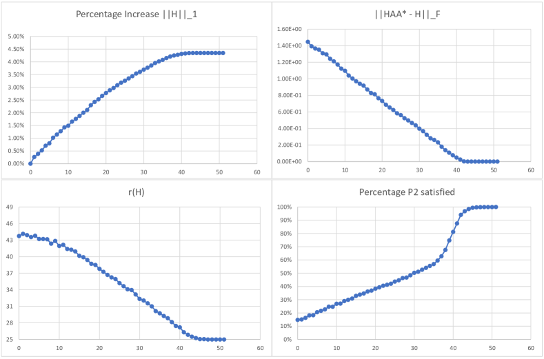
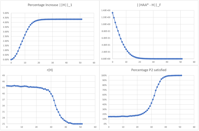
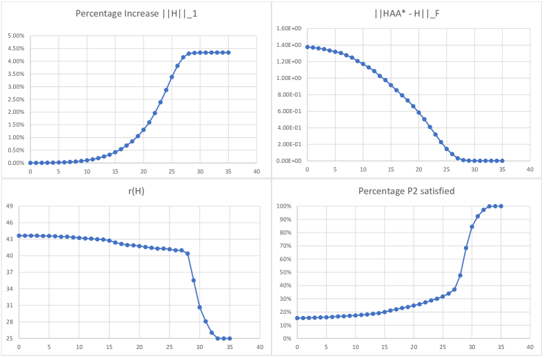
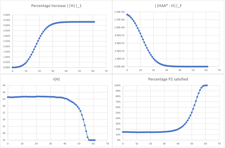
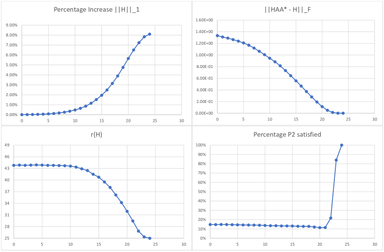
In Figures 3 to 7, we present plots to better show the behavior of the methods proposed as they iterate. The plots depict average values for $\widehat{\|H\|}_{1}$, $\|HAA^{\dagger}-H\|_{F}$, $r(H)$, and the percentage of the constraints in (3) that are satisfied.

Comparing the plots for the Cutting-plane method, in Figure 3, with the plots for Augmented Lagrangian, Penalized 1-norm and Penalized Frobenius, in Figures 4, 5, 6, we can more clearly observe that during the execution of Cutting-plane the rank starts to decrease when the 1-norm is still increasing and the percentage of constraints in (3) that are satisfied also increases faster from the beginning. The behavior of the solutions of the three other methods is very similar. Nevertheless, Penalized 1-norm shows a slightly better trade-off than the other two. We can observe a small decrease in the rank before the 1-norm achieves its optimal value. In Figure 7, we see that Nuclear-norm converges in fewer iterations than the other methods, but in terms of computational effort, it is the most expensive method, owing to the need to solve SDP problems. As guaranteed by the theory, all of the constraints (3) are satisfied when the rank is minimum, but only a few of them are satisfied until the last iterations. Despite this fact, the curves show the desired decrease in the rank as the 1-norm increases. However, as observed in Table 2 the 1-norm increases significantly more for this method than for the others. We have an increase of 8.1% in the 1-norm, while for the others it is only 4.3%.

Figure 3: Cutting-plane method

Figure 4: Augmented Lagrangian method

Figure 5: Penalized 1-norm method

Figure 6: Penalized Frobenius method

Figure 7: Nuclear-norm method

As Cutting-plane presented the best trade-off between the rank and the 1-norm of the solutions in the experiments discussed above, we further investigated if other ways of selecting the violated constraints to add to the problem at each iteration could improve even more the results. The best results were obtained when the violated constraints were selected randomly. So, in the following, we include in our analysis, a variation of Cutting-plane called Cutting-plane Random. Recall that for the original Cutting-plane, we consider the $nm$ equations (3), i.e., $H_{i\cdot}A(A^{\dagger})_{\cdot j}=H_{ij}$, lexically ordered by their indices $(j,i)$, with $i=1,\ldots,n$ and $j=1,\ldots,m$. At each iteration of Cutting-plane, we add the first $t$ equations that are violated by the current solution, to $P_{13}$. Alternatively, in Cutting-plane Random, we randomly reorder the indices $j$ or the indices $i$ before executing it. We execute the method twenty times, in the first ten, we randomly reorder $j$ and in the last ten, besides randomly reordering $i$, we search considering the lexical order of $(i,j)$. The solution of minimum 1-norm, for each rank found in the solutions is then presented. We will compare in the following Cutting-plane (CP), Cutting-plane Random (CP.Rand), Penalized 1-norm, and Nuclear-norm. The two other methods, Augmented Lagrangian and Penalized Frobenius, are not considered in the following because their behavior is very similar to Penalized 1-norm, only a bit worse.

	$\|H\|_{1}$				$\|H\|_{0}$
$r(H)$	Nuclear-norm	Pen.1-norm	CP	CP.Rand	Nuclear-norm	Pen.1-norm	CP	CP.Rand
48	(1, 0)	(1, 0)	(1, 1)	(1, 1)	(1, 0)	(1, 0)	(1, 1)	(1, 1)
47	(3, 0)	(3, 0)	(3, 2)	(3, 3)	(3, 0)	(3, 0)	(3, 2)	(3, 3)
46	(5, 1)	(5, 0)	(5, 2)	(5, 4)	(5, 0)	(5, 0)	(5, 3)	(5, 4)
45	(7, 0)	(5, 1)	(8, 3)	(8, 7)	(7, 0)	(5, 0)	(8, 4)	(8, 7)
44	(11, 0)	(9, 2)	(11, 3)	(11, 9)	(11, 0)	(9, 0)	(11, 5)	(11, 10)
43	(13, 0)	(8, 2)	(15, 6)	(15, 12)	(13, 0)	(8, 0)	(15, 8)	(15, 13)
42	(14, 1)	(11, 1)	(16, 3)	(16, 12)	(14, 0)	(11, 0)	(16, 7)	(16, 12)
41	(15, 0)	(12, 2)	(19, 5)	(19, 15)	(15, 0)	(12, 0)	(19, 7)	(19, 15)
40	(13, 1)	(9, 3)	(19, 3)	(19, 12)	(13, 1)	(9, 1)	(19, 8)	(19, 11)
39	(7, 0)	(8, 0)	(19, 5)	(19, 14)	(7, 0)	(8, 0)	(19, 8)	(19, 12)
38	(8, 0)	(3, 0)	(18, 2)	(19, 17)	(8, 0)	(3, 0)	(18, 4)	(19, 15)
37	(13, 0)	(4, 0)	(20, 5)	(20, 16)	(13, 0)	(4, 0)	(20, 9)	(20, 13)
36	(8, 0)	(5, 0)	(20, 3)	(20, 17)	(8, 0)	(5, 0)	(20, 7)	(20, 13)
35	(10, 0)	(5, 0)	(20, 1)	(20, 19)	(10, 0)	(5, 0)	(20, 7)	(20, 13)
34	(11, 0)	(4, 1)	(20, 1)	(20, 18)	(11, 0)	(4, 0)	(20, 7)	(20, 13)
33	(9, 0)	(5, 1)	(20, 1)	(20, 18)	(9, 0)	(5, 0)	(20, 8)	(20, 13)
32	(8, 0)	(6, 1)	(20, 1)	(20, 18)	(8, 0)	(6, 1)	(20, 8)	(20, 12)
31	(9, 0)	(5, 0)	(20, 1)	(20, 19)	(9, 0)	(5, 0)	(20, 8)	(20, 12)
30	(7, 0)	(5, 0)	(20, 1)	(20, 19)	(7, 0)	(5, 0)	(20, 5)	(20, 16)
29	(9, 0)	(8, 0)	(19, 4)	(20, 16)	(9, 0)	(8, 0)	(19, 11)	(20, 10)
28	(4, 0)	(12, 0)	(20, 3)	(20, 17)	(4, 0)	(12, 0)	(20, 5)	(20, 17)
27	(12, 0)	(6, 0)	(20, 2)	(20, 18)	(12, 0)	(6, 1)	(20, 6)	(20, 14)
26	(12, 0)	(12, 0)	(20, 3)	(20, 18)	(12, 0)	(12, 0)	(20, 6)	(20, 15)
25	(20, 0)	(20, 2)	(20, 6)	(20, 18)	(20, 0)	(20, 19)	(20, 17)	(20, 14)

Table 8: Number of instances where the methods find (at least one solution, the solution of minimum norm)

In Table 8, each row corresponds to the rank of at least one solution generated by the four methods when applied to our twenty instances. For each method, we show results concerning the 1-norm and the 0-norm of the solutions obtained. Each ordered pair presented in the table, contains the number of instances where the methods find at least one solution for the corresponding rank, and the number of instances where the method finds the least 1-norm (up to a tolerance of $10^{-4}$), for that rank, among all of the algorithms. A method for which the first coordinate is large indicates the ability of that method to generate a diverse set of solutions (i.e., with a variety of ranks), when trading-off rank against 1-norm. The second coordinate indicates when a method obtain the best solution among all for that rank, hence giving a nondominated solution, in the Pareto sense, considering the points $(\|H\|,r(H))$. From the results in Table 8, we observe:

• On average, the number of solutions of each rank is much smaller for Penalized 1-norm. Both Cutting-plane and Cutting-plane Random generates the same or nearly that same number of solutions of each rank, which are on average, much greater than the numbers for the other two methods.

• Nuclear-norm only obtains solutions of minimum 1-norm for three ranks, and for only one instance for each rank.

• Cutting-plane Random obtains the solution of minimum 1-norm in the vast majority of the cases, showing much superior results. The second best method is Cutting-plane.

• The results for the 0-norm are very similar to the results for the 1-norm, when analyzing Nuclear-norm and Penalized 1-norm, but when observing the the cutting-plane methods, we can see that the results are more balanced when comparing the 0-norms.

	$\|H\|_{1}$				$\|H\|_{0}$
Inst.	Nuclear-norm	Pen.1-norm	CP	CP.Rand	Nuclear-norm	Pen.1-norm	CP	CP.Rand
1	0	0	8	16	0	1	14	10
2	0	0	5	15	0	1	7	11
3	0	0	3	21	0	1	6	14
4	0	4	2	17	0	2	5	14
5	0	0	1	16	0	1	9	9
6	0	1	4	12	0	1	6	9
7	0	0	2	19	0	1	4	14
8	1	0	9	7	1	1	5	8
9	0	1	1	17	0	1	5	14
10	1	1	2	16	0	1	8	10
11	0	2	3	15	0	1	6	15
12	0	0	1	20	0	1	11	15
13	0	3	2	18	0	1	8	9
14	0	0	1	18	0	1	6	14
15	0	3	1	10	0	2	4	7
16	0	0	6	16	0	1	7	17
17	1	0	7	17	0	1	14	10
18	0	0	3	21	0	1	8	15
19	0	1	1	22	0	0	8	13
20	0	0	3	19	0	1	4	18

Table 9: Number of solutions nondominated by other methods

Table 9 presents results of the same experiments (as presented in Table 8), but now the rows indicate “instance” rather than “rank”, and we tabulate the number of nondominated solutions generated by instance, in the Pareto sense, considering the points $(\|H\|,r(H))$. We can clearly see that Cutting-plane Random is the best, with Cutting-plane also quite good. Penalized 1-norm generates a few points that are nondominated, and Nuclear norm rarely does.

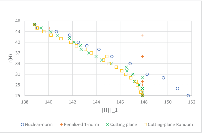
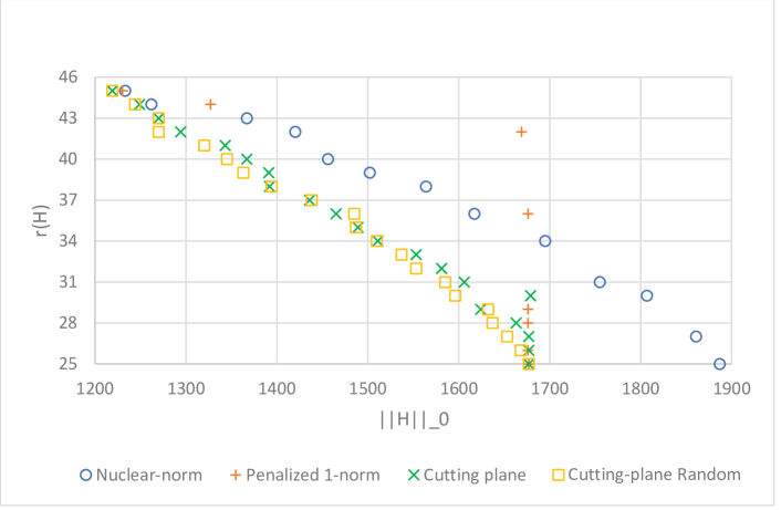
The plots in Figure 10 show the typical iterates generated by the four methods on one of our twenty random instances. These plots expand on the experiments summarized in “Row 16” of Table 9. We can see that Cutting-plane Random gives the best approximation of the Pareto curves, trading off 1/0-norms against rank. Nuclear-norm performs quite poorly at generating $H$ with low 1/0-norms for most ranks; it is particularly bad at the lower ranks. Even though Penalized 1-norm is overall quite poor, it can generate $H$ with decent 1/0-norms at very low and very high ranks. Overall the Cutting-plane methods are the clear winners, with Cutting-plane Random offering some improvement over Cutting-plane.

Figure 10: Pareto-curve approximations for an instance: four algorithms

4 Conclusion

There is a trade-off between 1-norm and sparsity against low-rank in the computation of ah-symmetric generalized inverses. These matrices can be applied in the solution of least-square problems, where low 1-norm, sparsity, and low-rank are all desirable features in their numerical applications. In this work, we propose algorithmic approaches to numerically analyze this trade-off, using the fact that a generalized inverse has minimum rank if and only if it satisfies the reflexive property. The algorithms start with a minimum 1-norm ah-symmetric generalized inverse and iteratively impose the reflexive property, gradually increasing 1-norm and decreasing rank, until the minimum rank is obtained. The intermediate solutions from these algorithms can represent the best trade-off between 1-norm and sparsity against rank in numerical applications. Among the different strategies proposed to gradually impose the reflexive property, the best trade-off between norms and rank is obtained by a cutting-plane method that solves linear-programming problems at each iteration, applying a linear re-formulation of the reflexive property, obtained when combining it with the other properties of ah-symmetric generalized inverses.