Scaling study of diffusion in dynamic crowded spaces

Abstract

We study Brownian motion in a space with a high density of moving obstacles in 1, 2 and 3 dimensions. Our tracers diffuse anomalously over many decades in time, before reaching a diffusive steady state with an effective diffusion constant $D_{\text{eff}}$ that depends on the obstacle density and diffusivity. The scaling of $D_{\text{eff}}$, above and below a critical regime at the percolation point for void space, is characterized by two critical exponents: the conductivity $\mu$, also found in models with frozen obstacles, and $\psi$, which quantifies the effect of obstacle diffusivity.

Introduction.

Brownian motion in disordered media has long been the focus of much theoretical and experimental work Havlin and Ben-Avraham (1987); Ben-Avraham and Havlin (2000). A particularly important application has more recently emerged, thanks to the ever increasing quality of microscopy techniques: that of transport inside the cell (see, e.g., Schwille et al. (1999); Smith et al. (1999); Dayel et al. (1999); Seisenberger et al. (2001) for some pioneering studies or Novak et al. (2009); Saxton (2012); Höfling and Franosch (2013); Mogre et al. (2020) for more recent overviews). Indeed, it is now possible to track the movement of single particles inside living cells, of sizes ranging from small proteins to viruses, RNA molecules or ribosomes. One generally considers the mean square displacement $\langle\Delta r^{2}(t)\rangle$ (MSD, the average of the squared distance traveled by the particle) and tries to fit it to a law of the form $\langle\Delta r^{2}(t)\rangle\propto t^{\alpha}$. Some experiments in prokaryotic cytoplasms Bakshi et al. (2011); Coquel et al. (2013) have found evidence for this behavior with $\alpha=1$, characteristic of the classical Brownian (or diffusive) motion Berg (1983). Many other works, however, have found signals of subdiffusive (i.e., $\alpha<1$) transport Golding and Cox (2006); Weber et al. (2010). In eukaryotic cells, where the environment is considerably more complex, heterogeneous and crowded, the range of observed behavior is even wider Bronstein et al. (2009); Jeon et al. (2011); Tabei et al. (2013).

On the theoretical front, a celebrated framework to generate anomalous diffusion is the continuum-percolation or “Swiss-cheese” model Halperin et al. (1985). In it, a large number of interpenetrating obstacles, usually spherical in shape, are randomly distributed throughout the system (see Figure 1). The behavior of tracer particles is controlled by the obstacle density. For low concentration, the long-time behavior is diffusive. When the percolation threshold Stauffer and Aharony (1994); Bollobás and Riordan (2006) is reached, however, the system undergoes a localization transition Saxton (1994); Höfling et al. (2006); Kammerer et al. (2008); Bauer et al. (2010); Spanner et al. (2011). The Swiss-cheese model is successful in generating (transient) anomalous diffusion in a crowded environment. From the point of view of cellular transport, however, it falls short in one important respect: it does not consider a dynamic medium, while cells are constantly rearranging themselves. This shortcoming has recently been addressed by considering Brownian obstacles Tremmel et al. (2003); Berry and Chaté (2014); Polanowski and Sikorski (2016); Nandigrami et al. (2017). In this case, the localization transition disappears and normal diffusion is reached at any obstacle density for long times. Most works, however, have concentrated on the transient subdiffusive regime rather than on the diffusive steady state.

Here we study Brownian motion in such a dynamic, crowded space and characterize how the long-time diffusive regime depends on obstacle density and mobility. Using extensive numerical simulations, we compute an effective diffusion constant $D_{\text{eff}}$ for a wide range of obstacle concentrations and diffusivities in one, two and three spatial dimensions. Even though, in accordance with previous work Tremmel et al. (2003); Berry and Chaté (2014), no localization transition is observed, we find that the percolation point still holds a special importance to define a critical scaling. In particular, the value of $D_{\text{eff}}$ is controlled by two critical exponents: the conductivity $\mu$ Adler (1985), which quantifies the approach to the critical density, and an exponent $\psi$, giving the scaling with the obstacle diffusivity.

Model and parameters.

In our model, which we implement in continuous spaces in spatial dimension $d=1,2$ and $3$, a volumeless particle takes a discrete-time random walk and encounters obstacles that block its path. The obstacles are uniformly-placed possibly-overlapping $d$-balls, an arrangement that in two dimensions has been called the Swiss-cheese model Halperin et al. (1985), see Fig. 1.

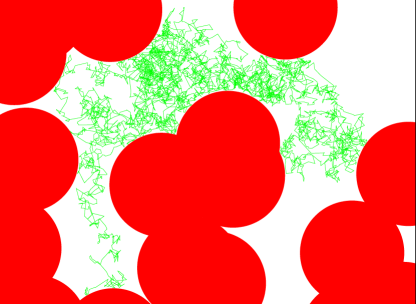
Figure 1: A particle traces a discrete-time random walk in two dimensions in green, blocked by frozen obstacles. At each time interval it draws a proposal for its new location from a centered Gaussian distribution. If offered a new position inside a red obstacle, the particle stays put for that timestep and attempts a new move at the following timestep. This arrangement of overlapping circular obstacles is commonly referred to as the Swiss-cheese model Halperin et al. (1985) in the case of immobile obstacles. Here, we consider the obstacles to be also Brownian particles, diffusing independently from one another.

At each timestep, our tracer particle takes a step in a random direction (chosen isotropically) of length extracted from a Gaussian distribution with standard deviation $\sigma_{\textnormal{p}}$. We set $\sigma_{\textnormal{p}}=1$ to define the unit length in the system. We are interested in unveiling the universal scaling properties of the long-time behavior of the tracers, so we do not need to model the interactions with the obstacles in microscopic detail. We simply have the particle stop if its proposed new location would be inside one of the obstacles. To avoid situations where the particle can jump over obstacles, we fix their radius as $R=10\gg\sigma_{\textnormal{p}}$.

The obstacles themselves also move, ignoring interactions and always drawing their discrete steps from a Gaussian distribution with standard deviation $\sigma_{\textnormal{obs}}\leq\sigma_{\textnormal{p}}$. To deal with situations where the void pocket inhabited by a particle becomes entirely squeezed, obstacles can “step on” particles, in which case the particle stops all motion until the obstacle moves off of it.

We are interested in how well the particle can explore the empty space, as measured by the mean square displacement (MSD) after $t$ timesteps,

$$\langle\Delta r^{2}(t)\rangle=\langle[\boldsymbol{r}(t+t_{0})-\boldsymbol{r}(t_{0})]^{2}\rangle.$$ (1)

As discussed in the introduction, when the MSD grows linearly with time, we say the motion is diffusive and characterize by a diffusion constant $D$, defined through the equation $\langle\Delta r^{2}(t)\rangle=2dDt$, where $d$ is the spatial dimension.

The first control parameter in this model is the dimensionless obstacle density, $\hat{n}=nR^{d}$, where $n$ is the number density of obstacle centers. In previous works in which the obstacles are frozen, at low obstacle densities the MSD is governed by three different behaviors at varying time scales Höfling et al. (2006); Bauer et al. (2010). These time scales have also been observed empirically in biological systems Saxton (2007).

In these cases, at microscopic time scales, particles do not encounter obstacles and diffuse freely. This gives us another characteristic parameter: the short-term diffusivity of the tracers, $D_{\text{p}}={\sigma_{\textnormal{p}}^{2}}/{2d}$. If there were no obstacles at all, we would recover $\langle\Delta r^{2}(t)\rangle=2dD_{\text{p}}t$.

At intermediate time scales, the system experiences subdiffusive motion, meaning $\langle\Delta r^{2}(t)\rangle\sim t^{\alpha},\alpha<1$. Finally, for long times the central limit theorem causes the MSD to revert to linear growth, $\langle\Delta r^{2}(t)\rangle\sim 2dD_{\text{eff}}t$ with $D_{\text{eff}}\ll D_{\text{p}}$ Höfling and Franosch (2013).

In frozen models, this third window of diffusive motion recedes as $\hat{n}$ approaches a critical value, $\hat{n}_{\text{c}}$, at which point it entirely disappears. This localization transition takes place at the percolation point $\hat{n}_{\text{c}}$ of the obstacles, when an infinite cluster partitions space into finite, disconnected pockets Stauffer and Aharony (1994); Bollobás and Riordan (2006). The critical scaling of $D_{\text{eff}}$ is controlled by a conductivity exponent $\mu$ Adler (1985); Grassberger (1999); Höfling et al. (2006)

$$D_{\text{eff}}\propto(\hat{n}_{\text{c}}-\hat{n})^{\mu},$$ (2)

with $D_{\textnormal{eff}}=0$ in the supercritical regime $\hat{n}\geq\hat{n}_{\text{c}}$. For $d=2$ and $3$, the critical density has been calculated to be $\hat{n}_{\text{c}}=0.359$ Quintanilla and Ziff (2007); Mertens and Moore (2012) and $0.839$ Yi and Esmail (2012), respectively. We also see that $\hat{n}_{\text{c}}=0$ trivially in $d=1$, because localization occurs once a single frozen obstacle appears.

In our model with moving obstacles, as has been observed Tremmel et al. (2003); Berry and Chaté (2014), particles never become localized because the obstacles themselves will eventually move out of the way. We expect, thus, to observe these three time windows at all obstacle densities, matching the biological observations. As we shall demonstrate, however, $\hat{n}_{\text{c}}$ still carries a special significance, so we continue to refer to $\hat{n}<\hat{n}_{\text{c}}$ ($\hat{n}>\hat{n}_{\text{c}}$) as the subcritical (supercritical) regime.

The second control parameter is the diffusivity of the obstacles, $D_{\text{obs}}$. This will generally be much lower than $D_{\text{p}}$  (otherwise, with our rules, the tracers’ movement would become enslaved to the obstacles). To optimize our simulations, we only move the obstacles every 10 time steps, giving us $D_{\textnormal{obs}}={\sigma_{\textnormal{obs}}^{2}}/{20d}$. As $D_{\text{obs}}\to 0$ we recover the frozen models .

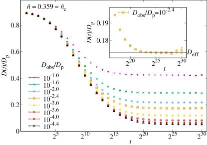
Figure 2: Time-dependent diffusion coefficient $D(t)$, eq. (3), in $d=2$ at approximately critical obstacle density for various obstacle diffusivities. Diffusivities are shown in units of the characteristic particle diffusivity $D_{\text{p}}$. In this representation, diffusive motion is characterized by a constant $D(t)$. Such a regime is always reached for long times in our model, no matter the obstacle density, defining an effective diffusion constant $D_{\text{eff}}$. The inset shows a closeup of the approach to this steady-state behavior for $D_{\text{obs}}/D_{\text{p}}=10^{-2.4}$. All curves in this plot are averaged over $24$ independent simulations, each with $360$ tracer particles.

Results in $d=2$.

We use a simulation box of linear size $L=1000$ with periodic boundary conditions. Given the annealed nature of our disorder, this is more than enough to avoid finite-size effects (see Appendix A). Since we are interested in the asymptotic behavior, we need to follow our tracers for a very long time in order to obtain good statistics. We use $1.2\times 10^{9}$ time steps. The MSD for each tracer is calculated according to eq. (1), for values of $t$ chosen as powers of 2 and letting $t_{0}$ range over multiples of $10^{6}$. Thus we averaged the distance traveled by a single particle across a shifting time window, with each $10^{6}$ steps as a different starting time. We gave the system a $10^{7}$ timestep “burn-in” period, in which data was not collected to allow the system to converge to its stationary distribution. We further improved our estimate of $\langle\Delta r^{2}(t)\rangle$ by launching 360 independent tracers in a single simulation, and ran 24 separate simulations for each pair of $\sigma_{\textnormal{obs}},\hat{n}$ values, so that the configuration and motion of obstacles can vary from system to system.

We describe the motion of the particle over time with a time-dependent diffusion coefficient,

$$D(t)=\frac{\langle\Delta r^{2}(t)\rangle}{2dt\phi}\ .$$ (3)

This definition is similar to that of Bauer et al. (2010), with one key difference: because some particles are trapped under obstacles at any given moment and therefore not moving, time must be rescaled by the proportion of particles that are free, or $\phi=\text{e}^{-\pi\hat{n}}$ in $d=2$ from the Poisson result . A similar argument was made in Novak et al. (2011a); *Novak2011b. This allows us to recover $D(t)\approx D_{\text{p}}$ for very small $t$, and also allows our results to approach the proper values in the limit of $D_{\text{obs}}\to 0$. Figure 2 displays the evolution of $D(t)$ over time for simulations at $\hat{n}\approx\hat{n}_{\text{c}}$ (similar plots in the sub- and supercritical regime are included in Appendix B). We are interested in the asymptotic value $D_{\text{eff}}=\lim_{t\to\infty}D(t)$, which, as discussed above, can be reached for any $\hat{n}$.

We estimate $D_{\text{eff}}$ by fitting $\langle\Delta r^{2}(t)\rangle$ to a constant for $t\geq 2^{29}$. Error bars are computed with a bootstrap method Young (2012). The resulting values are plotted in Figure 3. For $\hat{n}<\hat{n}_{\text{c}}=0.359$, as $D_{\text{obs}}\to 0$, $D_{\text{eff}}$ must eventually plateau at the values found by the frozen-obstacle models. On the other hand, for $\hat{n}\geq\hat{n}_{\text{c}}$, $\lim_{D_{\text{obs}}\to 0}D_{\text{eff}}=0$. As a consequence, in our log-log scale, curves for $\hat{n}<\hat{n}_{\text{c}}$ are concave and those for $\hat{n}>\hat{n}_{\text{c}}$ are convex. Remarkably, at precisely $\hat{n}_{\text{c}}$, $D_{\text{eff}}$ follows a power law

$$D_{\text{eff}}\propto D_{\text{obs}}^{\psi},\qquad\hat{n}=\hat{n}_{\text{c}}.$$ (4)

A fit to eq. (4) (see inset to Figure 4) yields $\psi=0.274(2)$ with and excellent goodness-of-fit value of $\chi^{2}/\textnormal{d.o.f.}=6.42/6$ [d.o.f. = degrees of freedom].

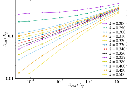
Figure 3: Effective diffusion coefficient against the diffusion coefficient of the obstacles for many obstacle densities in $d=2$. The percolation density is $\hat{n}_{\text{c}}\approx 0.359$.

Combining eq. (4) with eq. (2), we can formulate the following ansatz for the critical scaling in our model:

$$D_{\text{eff}}/D_{\text{p}} \simeq|\epsilon|^{\mu}\ g_{\pm}\bigl{[}(D_{\text{obs}}/D_{\text{p}})\ |\epsilon|^{-\mu/\psi}\bigr{]},$$ (5)

where $\epsilon=(\hat{n}-\hat{n}_{\text{c}})/{\hat{n}_{\text{c}}}$ and $g_{\pm}(x)$ are the scaling functions that describe the behavior in the sub- and supercritical regimes. Asymptotically, we expect $g_{\pm}(x)\sim x^{\psi}$ as $x\to\infty$, and $g_{-}(x)\sim\textnormal{const.}$ as $x\to 0$. Thus, in the subcritical regime, we recover eq. (2) as in studies with frozen obstacles. Using $\mu=1.3100(11)$ Grassberger (1999) and our previously computed $\psi$, eq. (5) collapses all our data without any adjustable parameters, see Figure 4.

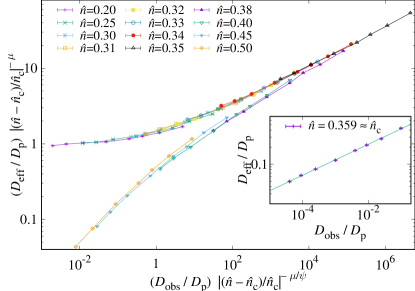
Figure 4: Scaling behavior in $d=2$ of $D_{\text{eff}}$ around the critical point, $\hat{n}_{\text{c}}\approx 0.359$, according to eq. (5). We take our value of the conductivity exponent, $\mu=1.31$, from Grassberger (1999). The dynamic exponent $\psi$ is computed with a critical fit to $D_{\text{eff}}\propto D_{\text{obs}}^{\psi}$ at $\hat{n}=\hat{n}_{\text{c}}$ (inset), yielding $\psi=0.274(2)$ with $\chi^{2}/\textnormal{d.o.f.}=6.42/6$. Using these exponents, the data collapse in the main panel, with separate branches for the supercritical and subcritical regimes, is achieved without adjustable parameters.

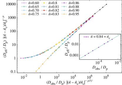
Figure 5: As in Figure 4, but in $d=3$. Now $\hat{n}_{\text{c}}\approx 0.84$ and $\mu\approx 2.88$ Machta and Moore (1985); Höfling et al. (2006). Our critical fit results in $\psi=0.520(3)$, with $\chi^{2}/\text{d.o.f.}=7.87/5$.

Results in $d=3$.

We ran analogous simulations in $d=3$. To keep the wall-clock of our runs under control, we reduced the simulation box to $L=200$, and launched 320 tracers in each system. To avoid finite-size effects we further slowed the obstacles by only moving them once every 100 steps. See Appendix 3 for an analog to Figure 3 in $d=3$. We follow the same procedure as in $d=2$ to compute $\psi=0.520(3)$.

One difference between $d=2$ and $d=3$ is that in the latter universality breaks down between lattice and continuum percolation models, so $\mu\neq\mu_{\textnormal{lat}}$ Halperin et al. (1985). There is, hence, some disagreement on the value of $\mu$ in $d=3$. Following the analysis in Machta and Moore (1985); Höfling et al. (2006) we have used $\mu=2.88$, which produces an excellent collapse of our data (see Figure 5).

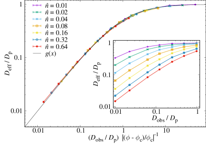
Figure 6: Effective diffusion constant in $d=1$. We plot our $D_{\text{eff}}$ rescaled according to eq. (6). Notice that now all densities $\hat{n}>0$ are supercritical. The inset shows the unscaled data.

Results in $d=1$.

The one-dimensional case has considerable theoretical interest. Now points become localized as soon as a single obstacle appears, so $\hat{n}_{\text{c}}=0$ and there is no subcritical regime. For our non-frozen model, particles are not localized because they can follow the obstacles as they move, or let an obstacle pass over them. We see, therefore, that $\psi=0$ trivially, because the particles can only diffuse when obstacles clear the way, so $D_{\text{eff}}$ is enslaved to $D_{\text{obs}}$.

In order to understand the scaling of $D_{\text{eff}}$ in $d=1$, we begin by considering several limits. First, when $\hat{n}\to 0$, $D_{\text{eff}}\to D_{\text{p}}$. Second, when $D_{\text{obs}}\to 0$ we approach the frozen limit with $D_{\text{eff}}=0$. Finally, $\lim_{\hat{n}\to\infty}D_{\text{eff}}=D_{\text{obs}}$. The latter is because, for dense enough obstacles, the tracer’s motion is entirely governed by how quickly the obstacles let it through. With these in mind, and remembering that $\phi=\text{e}^{-2\hat{n}}$, we propose the following ansatz: $D_{\text{eff}}={D_{\text{obs}}D_{\text{p}}}/[{D_{\text{p}}(1-\phi)+D_{\text{obs}}}]$. This is equivalent to using a different separation parameter than was used in $d=2$ and $d=3$, namely $\epsilon_{\phi}=(\phi-\phi_{\text{c}})/\phi_{\text{c}}=\phi-1$, and writing

$$D_{\text{eff}}/D_{\text{p}}=g\bigl{[}(D_{\text{obs}}/D_{\text{p}})\ |\epsilon_{\phi}|^{-1}\bigr{]},\qquad g(x)=\frac{x}{1+x}.$$ (6)

Figure 6 shows that eq. (6) is an excellent match to our data in a very wide range of $\phi$.

Conclusions.

We have performed a comprehensive investigation of diffusion in the void space of a dynamic version of the Swiss-cheese model in dimensions one through three. We have characterized the critical point governing the anomalous diffusion using two exponents, one of which is the traditional conductivity exponent $\mu$ and the other of which we call $\psi$. The latter exponent describes scaling of the effective diffusivity at precisely the critical obstacle density. For dimensions one through three we find $\psi=0$, $\psi=0.274(2)$ and $\psi=0.520(3)$, respectively.

Together, $\mu$ and $\psi$ can be used to encode the quantitative behavior of the system for a wide range of obstacle densities and diffusivities. This scaling is expected to be universal and covers several orders of magnitude in the mobility of the obstacles, so it should be directly relevant to the interpretation of cellular transport and other experiments on crowded spaces.

Appendix A Finite-Size Effects

Our model does not suffer from strong finite-size effects, probably thanks to the annealed nature of the disorder. Therefore, our simulations for $L=1000$ should be representative of the large-$L$ limit. We have, nevertheless, explicitly checked against finite-size effects by repeating our $\hat{n}=\hat{n}_{\text{c}}$ simulations for a smaller system size ($L=500$) and verifying that we get the same $D(t)$ curve as in Figure 2. This is shown in Figure 8. For all $D_{\text{obs}}$ the resulting $D_{\text{eff}}$ is the same in the $L=500$ system, but the data is noisier. Moreover, ultimately the strongest proof for the absence of finite-size effects is the fact that the power-law fits in Figures 4 and 5 satisfy a $\chi^{2}$ test.

Appendix B Time evolution in the sub- and supercritical regimes

Figure 2 shows $D(t)$ for many obstacle diffusivities at $\hat{n}\approx\hat{n}_{\text{c}}$. In Figures 8 and 10 we reproduce the same plot for a subcritical density ($\hat{n}=0.2$) and a supercritical one ($\hat{n}=0.4$). The resulting plots are qualitatively the same as Figure 2. Notice in particular that, even in the supercritical case, above the percolation point, the diffusive regime is eventually reached.

Appendix C Unscaled $D_{\text{eff}}$ in $d=3$

The time-dependent diffusion coefficient $D(t)$ and the effective diffusivity $D_{\text{eff}}$ have qualitatively the same behavior in $d=3$ as in $d=2$, but $D_{\text{eff}}$ is governed by different scaling exponents, as shown in Figure 5. In Figure 10 we plot the unscaled $D_{\text{eff}}$ for all our $d=3$ simulations.

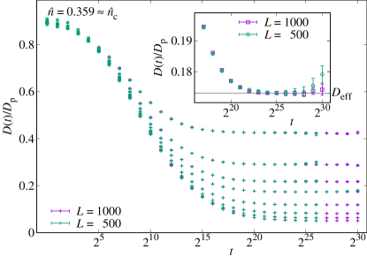
Figure 7: Same as Figure 2, but adding data for a smaller system size ($L=500$). Since the curves for $L=1000$ and $L=500$ are identical for the whole $t$ range, we have only plotted most of the small simulations up to $t=2^{26}$ for visualization purposes. The exception is $D_{\text{obs}}/D_{\text{p}}=10^{-2.4}$, enlarged in the inset. The $L=500$ curve are noisier for long $t$ where there are few $t_{0}$ to compute the MSD.

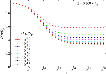
Figure 8: Same as Figure 2, but for a subcritical obstacle concentration ($\hat{n}=0.2$).

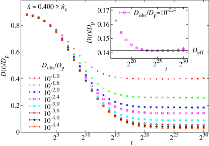
Figure 9: Same as Figure 2, but for a supercritical obstacle concentration ($\hat{n}=0.4$). The inset shows that the long-time diffusive regime [constant $D(t)$] is clearly reached.

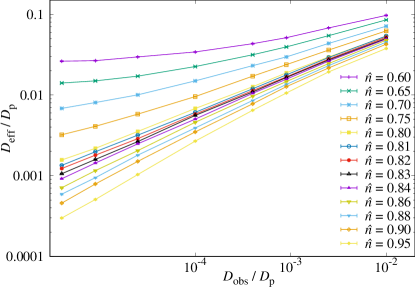
Figure 10: Effective diffusion coefficient against the diffusion coefficient of the obstacles for many obstacle densities in $d=3$. The percolation density is $\hat{n}_{\text{c}}\approx 0.839$.

References

- Havlin and Ben-Avraham (1987) S. Havlin and D. Ben-Avraham, “Diffusion in disordered media,” Adv. Phys. 36, 695 (1987).
- Ben-Avraham and Havlin (2000) D. Ben-Avraham and S. Havlin, Diffusion and Reactions in Fractals and Disordered Systems (Cambridge University Press, Cambridge, 2000).
- Schwille et al. (1999) P. Schwille, J. Korlach, and W. W. Webb, “Fluorescence correlation spectroscopy with single-molecule sensitivity on cell and model membranes,” Cytometry 36, 176 (1999).
- Smith et al. (1999) P. R. Smith, I. E. G. Morrison, K. M. Wilson, N. Fernández, and R. J. Cherry, “Anomalous diffusion of major histocompatibility complex class I molecules on HeLa cells determined by single particle tracking,” Biophys. J. 76, 3331 (1999).
- Dayel et al. (1999) M. J. Dayel, E. F. Y. Hom, and A. S. Verkman, “Diffusion of green fluorescent protein in the aqueous-phase lumen of endoplasmic reticulum,” Biophys. J. 76, 2843 (1999).
- Seisenberger et al. (2001) G. Seisenberger, M. U. Ried, T. Endreß, H. Büning, M. Hallek, and C. Bräuchle, “Real-time single-molecule imaging of the infection pathway of an adeno-associated virus,” Science 294, 1929 (2001).
- Novak et al. (2009) I. L. Novak, P. Kraikivski, and B. M. Slepchenko, “Diffusion in cytoplasm: Effects of excluded volume due to internal membranes and cytoskeletal structures,” Biophys. J. 97, 758 (2009).
- Saxton (2012) M. J. Saxton, “Wanted: A positive control for anomalous subdiffusion,” Biophys. J. 103, 2411 (2012).
- Höfling and Franosch (2013) F. Höfling and T. Franosch, “Anomalous transport in the crowded world of biological cells,” Rep. Prog. Phys. 76, 046602 (2013).
- Mogre et al. (2020) S. S. Mogre, A. I. Brown, and E. F. Koslover, “Getting around the cell: physical transport in the intracellular world,” Phys. Biol. 17, 061003 (2020).
- Bakshi et al. (2011) S. Bakshi, B. P. Bratton, and J. C. Weisshaar, “Subdiffraction-limit study of Kaede diffusion and spatial distribution in live escherichia coli,” Biophys. J. 101, 2535 (2011).
- Coquel et al. (2013) A.-S. Coquel, J.-P. Jacob, M. Primet, A. Demarez, M. Dimiccoli, T. Julou, L. Moisan, A. B. Lindner, and H. Berry, “Localization of protein aggregation in escherichia coli is governed by diffusion and nucleoid macromolecular crowding effect,” PLoS Comput. Biol. 9, 1 (2013).
- Berg (1983) H. C. Berg, Random Walks in Biology (Princeton University Press, Princeton, 1983).
- Golding and Cox (2006) I. Golding and E. C. Cox, “Physical nature of bacterial cytoplasm,” Phys. Rev. Lett. 96, 098102 (2006).
- Weber et al. (2010) S. C. Weber, A. J. Spakowitz, and J. A. Theriot, “Bacterial chromosomal loci move subdiffusively through a viscoelastic cytoplasm,” Phys. Rev. Lett. 104, 238102 (2010).
- Bronstein et al. (2009) I. Bronstein, Y. Israel, E. Kepten, S. Mai, Y. Shav-Tal, E. Barkai, and Y. Garini, “Transient anomalous diffusion of telomeres in the nucleus of mammalian cells,” Phys. Rev. Lett. 103, 018102 (2009).
- Jeon et al. (2011) J.-H. Jeon, V. Tejedor, S. Burov, E. Barkai, C. Selhuber-Unkel, K. Berg-Sørensen, L. Oddershede, and R. Metzler, “In vivo anomalous diffusion and weak ergodicity breaking of lipid granules,” Phys. Rev. Lett. 106, 048103 (2011).
- Tabei et al. (2013) S. M. A. Tabei, S. Burov, H. Y. Kim, A. Kuznetsov, T. Huynh, J. Jureller, L. H. Philipson, A. R. Dinner, and N. F. Scherer, “Intracellular transport of insulin granules is a subordinated random walk,” Proc. Natl. Acad. Sci. USA 110, 4911 (2013).
- Halperin et al. (1985) B. I. Halperin, S. Feng, and P. N. Sen, “Differences between lattice and continuum percolation transport exponents,” Phys. Rev. Lett. 54, 2391 (1985).
- Stauffer and Aharony (1994) D. Stauffer and A. Aharony, Introduction to percolation theory, 2nd ed. (Taylor & Francis, 1994).
- Bollobás and Riordan (2006) B. Bollobás and O. Riordan, Percolation (Cambridge University Press, Cambridge, 2006).
- Saxton (1994) M. J. Saxton, “Anomalous diffusion due to obstacles: a Monte Carlo study,” Biophys. J. 66, 394 (1994).
- Höfling et al. (2006) F. Höfling, T. Franosch, and E. Frey, “Localization transition of the three-dimensional Lorentz model and continuum percolation,” Phys. Rev. Lett. 96, 165901 (2006).
- Kammerer et al. (2008) A. Kammerer, F. Höfling, and T. Franosch, “Cluster-resolved dynamic scaling theory and universal corrections for transport on percolating systems,” Europhys. Lett. 84, 66002 (2008).
- Bauer et al. (2010) T. Bauer, F. Höfling, T. Munk, E. Frey, and T. Franosch, “The localization transition of the two-dimensional Lorentz model,” Eur. Phys. J. Special Topics 189, 103 (2010).
- Spanner et al. (2011) M. Spanner, F. Höfling, G. E. Schröder-Turk, K. Mecke, and T. Franosch, “Anomalous transport of a tracer on percolating clusters,” J. Phys.: Condens. Matter 23, 234120 (2011).
- Tremmel et al. (2003) I. G. Tremmel, H. Kirchhoff, and G. D. Farquhar, “Dependence of plastoquinol diffusion on the shape, size, and density of integral thylakoid proteins,” Biochim. Biophys. Acta 1607, 97 (2003).
- Berry and Chaté (2014) H. Berry and H. Chaté, “Anomalous diffusion due to hindering by mobile obstacles undergoing Brownian motion or Orstein-Ulhenbeck processes,” Phys. Rev. E 89, 022708 (2014).
- Polanowski and Sikorski (2016) P. Polanowski and A. Sikorski, “Simulation of molecular transport in systems containing mobile obstacles,” J. Phys. Chem. B 120, 7529 (2016).
- Nandigrami et al. (2017) P. Nandigrami, B. Grove, A. Konya, and R. L. B. Selinger, “Gradient-driven diffusion and pattern formation in crowded mixtures,” Phys. Rev. E 95, 022107 (2017).
- Adler (1985) J. Adler, “Conductivity exponents from the analysis of series expansions for random resistor networks,” J. Phys. A: Math. Gen. 18, 307 (1985).
- Saxton (2007) M. J. Saxton, “A biological interpretation of transient anomalous subdiffusion. i. qualitative model,” Biophys. J. 92, 1178 (2007).
- Grassberger (1999) P. Grassberger, “Conductivity exponent and backbone dimension in 2-d percolation,” Physica A 262, 251 (1999).
- Quintanilla and Ziff (2007) J. A. Quintanilla and R. M. Ziff, “Asymmetry in the percolation thresholds of fully penetrable disks with two different radii,” Phys. Rev. E 76, 051115 (2007).
- Mertens and Moore (2012) S. Mertens and C. Moore, “Continuum percolation thresholds in two dimensions,” Phys. Rev. E 86, 061109 (2012).
- Yi and Esmail (2012) Y. B. Yi and K. Esmail, “Computational measurement of void percolation thresholds of oblate particles and thin plate composites,” J. Appl. Phys. 111, 124903 (2012).
- Note (1) We have checked this explicitly by computing fits to (2\@@italiccorr) and checking that our is compatible with the values in the literature.
- Note (2) Equivalently, in and in , reflecting the equations for the volumes of 1-balls and 3-balls respectively.
- Novak et al. (2011a) I. L. Novak, F. Gao, P. Kraikivski, and B. M. Slepchenko, “Diffusion amid random overlapping obstacles: Similarities, invariants, approximations,” J. Chem. Phys. 134, 154104 (2011a).
- Novak et al. (2011b) I. L. Novak, F. Gao, P. Kraikivski, and B. M. Slepchenko, “Erratum: Diffusion amid random overlapping obstacles: Similarities, invariants, approximations,” J. Chem. Phys. 135, 039901 (2011b).
- Young (2012) A. P. Young, “Everything you wanted to know about data analysis and fitting but were afraid to ask,” (2012), arXiv:1210.3781 .
- Machta and Moore (1985) J. Machta and S. M. Moore, “Diffusion and long-time tails in the overlapping Lorentz gas,” Physical Review A 32, 3164 (1985).