Temporal boundaries in electromagnetic materials

Abstract

Temporally modulated optical media are important in both abstract and applied applications, such as spacetime transformation optics, relativistic laser-plasma interactions, and dynamic metamaterials. Here we investigate the behaviour of temporal boundaries, and show that traditional approaches that assume constant dielectric properties, with loss incorporated as an imaginary part, necessarily lead to unphysical solutions. Further, although physically reasonable predictions can be recovered with a narrowband approximation, we show that appropriate models should use materials with a temporal response and dispersive behaviour.

I Introduction

Mobile technologies are considered the biggest technology platform in history, with transformative advances occurring across all society. These are having a profound impact in diverse areas including health care, education, and industry [1]. Key to developing mobile technologies is the ability to predict electromagnetic (EM) wave propagation though systems with differing permittivities, and in particular predicting losses. In both physics [2] and engineering [3], EM loss is often expressed using the electric loss tangent (“$\tan\delta$”), the ratio of the imaginary to the real part of the permittivity. This constant permittivity model is widely used in condensed matter physics [2], and is critical to the design of technologies diverse as mobile phones, imaging systems, consumer electronics, radar, accelerators, sensors, and even microwave therapy [4]. In such situations, microscopic models involving e.g. atomic structure or quantum mechanical effects typically provide no significant advantage.

As new materials are developed for use in novel devices, it becomes vital that EM loss and propagation are correctly predicted. A very exciting new concept is time dependent media, where abrupt changes in permittivity can create a temporal boundary. Boundaries play a key role in many physical models; they provide initial and final states in dynamical systems, constrain analytic solutions in confined systems, and represent transitions between different modes of operation. These concepts date back to the 1950s, when Morgenthaler [5] showed that a temporal change of the permittivity produces both forward and backward propagating waves; a result echoed in directional formulations for wave propagation [6, 7, 8, 9, 10]. Temporal boundaries [5, 11, 12, 13] act as time-reversing mirrors in acoustics [14]; in EM an instantaneous time mirror with a sign-change in permittivity has been predicted [15] to cause field amplification. Other examples include dynamically configurable systems [16, 17], spacetime transformation devices [18, 19, 20, 21], time crystals [22, 23, 24], “field patterns” [25], and in laser driven plasma where relativistic changes can lead to a spatial and temporally varying permittivity.

Here we prove that modelling loss using a constant complex permittivity and permeability [26, 27, 15, 28] is physically incompatible with a temporal boundary. Such models can lead to unphysical post-boundary solutions that grow exponentially, despite being applied to passive and lossy materials; or fields may become complex-valued despite being real-valued before. This important point, which provides an unambiguous warning to non-specialists, is not addressed in other recent work on temporal boundaries, which focus on either reflection and refraction inside a medium with parabolic dispersion [29], appropriately generalised Kramers Kronig relations [30], or the complicated effects resulting from a Lorentzian response model [31]. Our dynamic material model, in contrast to more complicated ones [30, 31] is explicitly designed to provide a minimal example with simple behaviour which clearly reveals the basic physical principles relating to the treatment of temporal boundaries: the necessity of considering the dynamics of the bound current, the requirement for material-property boundary conditions, and the resulting secondary implications for frequency-domain properties such as the dispersion relations.

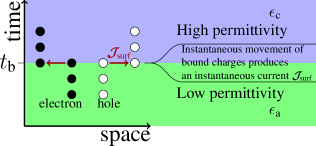
Figure 1: A temporal boundary or transition based on fundamental TBCs. Here, a sudden increase of permittivity at $t={{{{t_{{\textup{b}}}}}}}$, represented as the movement of bound charges, necessarily generates a microscopic “time-surface” current ${\boldsymbol{\mathcal{J}}_{\!\!\textup{surf}}}$.

In this article the term “boundary” refers to an interface between two regions with different constitutive relations (CRs). In electromagnetism CRs are most simply given by a permittivity $\epsilon$ and permeability $\mu$, although more complicated CRs are also allowed. In contrast to spatial boundary conditions that describe an interface between two static media, here we consider a temporal boundary at ${t_{{\textup{b}}}}$, where the medium has one set of CR properties before the transition ($t<{t_{{\textup{b}}}}$), and different CRs afterwards ($t>{t_{{\textup{b}}}}$). In our idealised transition, the CR for the entire region changes instantly; although gradual transitions are also possible [32, 33]. The unphysical consequences arise irrespective of which of the two possible types of temporal boundary condition (TBC) we consider. The first “natural” TBC [34] is derived from Maxwell’s equations on the assumption that all the currents are finite, which leads to the continuity of ${\boldsymbol{D}}$ and ${\boldsymbol{B}}$. The second “fundamental” TBC treats only ${\boldsymbol{E}}$ and ${\boldsymbol{B}}$ as physical EM fields, with ${\boldsymbol{D}}$ and ${\boldsymbol{H}}$ as derived fields acting as a gauge for the current [35, 36, 37]; here ${\boldsymbol{E}}$ and ${\boldsymbol{B}}$ are also continuous, but a temporal-surface dipole current appears at the transition, as shown in Fig. 1.

After demonstrating and defining the problem, we present two methods for obtaining physically meaningful solutions. The first applies the constant complex CR model whilst using a narrow band approximation (NBA). This leads to a solution based on complex conjugate pairs of frequencies and refractive indices. Although partially successful, it merely hides the fact that to model lossy media correctly when there is a temporal boundary, one requires a time-dependent material response, and therefore dispersive CR, where $\epsilon$ and/or $\mu$ depend on frequency. Besides, just as a dynamic medium model requires its own fields to represent its state, in the frequency domain we see that a dispersive medium generates one or more additional modes; and this necessary information cannot be included in the standard constant complex CR model. Thus in either time or frequency, additional boundary conditions (ABCs) must be specified.

Note that proofs and additional discussion are presented in the Supplementary Material following the References.

II Linear Media

In linear media any EM field can be represented in the Fourier domain by a sum or integral of terms of the form $\exp({-i\omega t+i{\boldsymbol{k}}\cdot{\boldsymbol{x}}})$, where $\omega\in{\mathbb{C}}$ is a complex frequency, and ${\boldsymbol{k}}\in{\mathbb{C}}^{3}$ a complex wavevector. Since the source free Maxwell’s equations (5) are linear, with ${\boldsymbol{J}}_{\!\textup{total}}=0$ and $\rho=0$, it is sufficient to consider just a single mode

$$E_{x}(t,z)=E_{0}\exp({-i\omega t+ikz})\quad\textup{where}\quad k\,,\omega\in{\mathbb{C}},$$ (1)

with ${\boldsymbol{k}}$ oriented along the $z$-axis (along $\hat{\boldsymbol{z}}$), and ${\boldsymbol{E}}$ along $\hat{\boldsymbol{x}}$.

Now consider a temporally dispersive medium where the CRs specify permittivity ${\widetilde{\epsilon}}(-\omega)$ and permeability $\mu_{{\scalebox{0.6}{0}}}$, and where the “$-\omega$” is a consequence of choosing $e^{-i\omega t}$ in (1). If $\omega$ and ${\widetilde{\epsilon}}(-\omega)$ are both real then ${\widetilde{\epsilon}}(-\omega)$ can be replaced with ${\widetilde{\epsilon}}(\omega)$; but this is not allowed in our following calculations, because extra care must be taken when using complex permittivity to model damping. From Maxwell (5) we obtain a dispersion relation, and define the refractive index[38, 39, 40]. These are

$$k^{2}-\omega^{2}\ \mu_{{\scalebox{0.6}{0}}}\,{\widetilde{\epsilon}}(-\omega) =0,$$ (2)

$${\tilde{{n}}}(-\omega)^{2} ={c_{{\scalebox{0.6}{0}}}^{2}}\,\mu_{{\scalebox{0.6}{0}}}\,{\widetilde{\epsilon}}(-\omega),$$ (3)

where ${c_{{\scalebox{0.6}{0}}}}=(\epsilon_{{\scalebox{0.6}{0}}}\mu_{{\scalebox{0.6}{0}}})^{-1/2}$ is the vacuum speed of light.

We now ask whether these CRs correspond to a passive lossy medium, i.e. one dampened with no external energy added. Given that both $\omega$ and $k$ can be either real or complex, there are two possibilities that are straightforward to consider. These fit into the temporally propagated and spatially propagated viewpoints respectively [41], and are:

First, if $\omega$ is real and positive, we require that plane waves are spatially evanescent in the propagation direction, which implies ${\textup{Im}}\big{(}{\widetilde{\epsilon}}(-\omega)\big{)}>0$.

Second, if $k$ is real, then we need ${\textup{Im}}(\omega)<0$ to damp the field, leading to the requirement that when $\omega^{2}{\widetilde{\epsilon}}(-\omega)$ is real and positive, then ${\textup{Im}}(\omega)<0$.

How the fields represented by these modes, change as they cross a temporal boundary will depend on how the change in CRs is specified, and on the chosen TBCs.

III Temporal Boundary Conditions

Different types of electromagnetic TBC can be identified, depending on the material response [11, 12, 42]; here we summarise focussing on how bound currents represent the material response. First, as depicted in Fig. 1, we could identify the sudden change in the CRs at $t={t_{{\textup{b}}}}$ as leading to an instantaneous temporal-surface dipole current (${\boldsymbol{\mathcal{J}}_{\!\!\textup{surf}}}$). The total current, ${\boldsymbol{J}}_{\!\textup{total}}$, in the medium is

$${\boldsymbol{J}}_{\!\textup{total}} ={\boldsymbol{J}}_{\!\textup{reg}}-\delta(t-{{t_{{\textup{b}}}}})\,{\boldsymbol{\mathcal{J}}_{\!\!\textup{surf}}},$$ (4)

where ${\boldsymbol{J}}_{\!\textup{reg}}$ is the usual finite current in Maxwell’s equations:

$$\begin{gathered}\nabla\cdot{\boldsymbol{B}}=0\,,\quad\nabla\cdot{\boldsymbol{D}}=\rho\\ \nabla\times{\boldsymbol{E}}+\partial_{t}{{\boldsymbol{B}}}=0\quad\textup{and}\quad\nabla\times{\boldsymbol{H}}-\partial_{t}{{\boldsymbol{D}}}={\boldsymbol{J}}_{\!\textup{total}}.\end{gathered}$$ (5)

Since the fields ${\boldsymbol{E}},{\boldsymbol{B}},{\boldsymbol{D}},{\boldsymbol{H}}$ may be discontinuous we write

$${\boldsymbol{D}}(t,{\boldsymbol{x}}) =\theta({{t_{{\textup{b}}}}}-t)\,{\boldsymbol{D}}_{\textup{a}}(t,{\boldsymbol{x}})+\theta(t-{{t_{{\textup{b}}}}})\,{\boldsymbol{D}}_{\textup{c}}(t,{\boldsymbol{x}})$$ (6)

where ${\boldsymbol{D}}_{\textup{a}}$ and ${\boldsymbol{D}}_{\textup{c}}$ are the ${\boldsymbol{D}}$ before and after the transition and $\theta$ is the Heaviside function. Using (4) and (6) in the Maxwell-Ampère equation, we have

$${\boldsymbol{J}}_{\!\textup{total}} ={\boldsymbol{J}}_{\!\textup{reg}}-\delta(t-{{t_{{\textup{b}}}}}){\boldsymbol{\mathcal{J}}_{\!\!\textup{surf}}}=\nabla\times{\boldsymbol{H}}-\partial_{t}{{\boldsymbol{D}}}$$

$$=\theta({{t_{{\textup{b}}}}}-t)\nabla\times{\boldsymbol{H}}_{{\textup{a}}}(t,{\boldsymbol{x}})+\theta(t-{{t_{{\textup{b}}}}})\nabla\times{\boldsymbol{H}}_{{\textup{c}}}(t,{\boldsymbol{x}})$$

$$\qquad-\theta({{t_{{\textup{b}}}}}-t)\partial_{t}{\boldsymbol{D}}_{{\textup{a}}}(t,{\boldsymbol{x}})-\theta(t-{{t_{{\textup{b}}}}})\partial_{t}{\boldsymbol{D}}_{{\textup{c}}}(t,{\boldsymbol{x}})$$

$$\qquad-\delta(t-{{t_{{\textup{b}}}}})\big{\{}{\boldsymbol{D}}_{{\textup{c}}}(t,{\boldsymbol{x}})-{\boldsymbol{D}}_{{\textup{a}}}(t,{\boldsymbol{x}})\big{\}}.$$

This approach can also be used for ${\boldsymbol{B}}$ in the Maxwell-Faraday equation to derive a similar result. The TBC are

$$[{\boldsymbol{D}}]={\boldsymbol{\mathcal{J}}_{\!\!\textup{surf}}}\qquad\textup{and}\qquad[{\boldsymbol{B}}]=0,$$ (7)

where $[{\boldsymbol{D}}]={\boldsymbol{D}}_{{\textup{c}}}({t_{{\textup{b}}}},{\boldsymbol{x}})-{\boldsymbol{D}}_{{\textup{a}}}({t_{{\textup{b}}}},{\boldsymbol{x}})$, etc. One option [5, 15] is to set ${\boldsymbol{\mathcal{J}}_{\!\!\textup{surf}}}=0$, to obtain the natural TBC, i.e.

$$[{\boldsymbol{D}}]=0\qquad\textup{and}\qquad[{\boldsymbol{B}}]=0.$$ (8)

Alternatively, if treating ${\boldsymbol{E}}$ and ${\boldsymbol{B}}$ as the only physical fields, we get the fundamental TBC, i.e.

$$[{\boldsymbol{E}}]=0\qquad\textup{and}\qquad[{\boldsymbol{B}}]=0,$$ (9)

which rely on (7) to calculate the conserved temporal-surface current ${\boldsymbol{\mathcal{J}}_{\!\!\textup{surf}}}$. This is an analogous approach to that describing the surface current around a permanent magnet [35].

IV Constant Complex CR gives Unphysical Results

Even a time boundary between a vacuum with $\epsilon=\epsilon_{{\scalebox{0.6}{0}}}$ and a lossy medium with $\epsilon={\epsilon_{{\textup{c}}}}$, where ${\epsilon_{{\textup{c}}}}$ is a non real constant with ${\textup{Im}}({\epsilon_{{\textup{c}}}})<0$ and ${\textup{Re}}({\epsilon_{{\textup{c}}}})>0$, results in a failure. For simplicity, we set ${t_{{\textup{b}}}}=0$, so that ${\boldsymbol{D}}(t,{\boldsymbol{x}})=\epsilon_{\scalebox{0.6}{0}}\,{\boldsymbol{E}}(t,{\boldsymbol{x}})$ for $t<0$, and ${\boldsymbol{D}}(t,{\boldsymbol{x}})={\epsilon_{{\textup{c}}}}\,{\boldsymbol{E}}(t,{\boldsymbol{x}})$ for $t>0$; and then choose a field polarization so that ${\boldsymbol{E}}=E_{x}(t,z)\hat{\boldsymbol{x}}$, and ${\boldsymbol{B}}=B_{y}(t,z)\hat{\boldsymbol{y}}$.

Pre-boundary ($t<{0}$), we start with a single real mode

$$E_{x}(t,z) =E_{{\scalebox{0.6}{0}}}\cos({\omega_{{\textup{a}}}t-k_{{\textup{a}}}z}),$$ (10)

with $E_{{\scalebox{0.6}{0}}}\in{\mathbb{R}}$ and $B_{y}(t,z)=E_{x}/{c_{{\scalebox{0.6}{0}}}}$. Here $\omega_{{\textup{a}}},k_{{\textup{a}}}$ are both real and positive and satisfy the vacuum dispersion relation ${c_{{\scalebox{0.6}{0}}}^{2}}k_{{\textup{a}}}^{2}=\omega_{{\textup{a}}}^{2}$. Since the post-boundary lossy material, with $\omega_{{\textup{c}}}$ and $k_{{\textup{c}}}$, must have ${\textup{Im}}({\epsilon_{{\textup{c}}}})>0$, the $t>{0}$ general solution is

$$E_{x}(t,z) =\left({g^{-}_{+}}\,e^{-i\omega_{{\textup{c}}}t+ik_{{\textup{c}}}z}+{g^{-}_{-}}\,e^{-i\omega_{{\textup{c}}}t-ik_{{\textup{c}}}z}\right.$$ (11)

$$\qquad+\left.{g^{+}_{-}}\,e^{i\omega_{{\textup{c}}}t-ik_{{\textup{c}}}z}+{g^{+}_{+}}\,e^{i\omega_{{\textup{c}}}t+ik_{{\textup{c}}}z}\right),$$

$$B_{y}(t,z) =\frac{{k_{{\textup{c}}}}}{{\omega_{{\textup{c}}}}}\left({g^{-}_{+}}\,e^{-i\omega_{{\textup{c}}}t+ik_{{\textup{c}}}z}-{g^{-}_{-}}\,e^{-i\omega_{{\textup{c}}}t-ik_{{\textup{c}}}z}\right.$$

$$\quad\qquad+\left.{g^{+}_{-}}\,e^{i\omega_{{\textup{c}}}t-ik_{{\textup{c}}}z}-{g^{+}_{+}}\,e^{i\omega_{{\textup{c}}}t+ik_{{\textup{c}}}z}\right),$$

with the dispersion relation

$${k_{{\textup{c}}}}{c_{{\scalebox{0.6}{0}}}}={n_{{\textup{c}}}}{\omega_{{\textup{c}}}}\qquad\textup{where}\qquad n_{{\textup{c}}}=c_{{\scalebox{0.6}{0}}}({\epsilon_{{\textup{c}}}}\mu_{{\scalebox{0.6}{0}}})^{1/2}.$$ (12)

The choice of root for ${n_{{\textup{c}}}}$ is unimportant, as both roots are included in (11). The first root ${\textup{Re}}(n_{{\textup{c}}})>0$, since ${\textup{Im}}({\epsilon_{{\textup{c}}}})>0$, requires ${\textup{Im}}(n_{{\textup{c}}})>0$; and the second root ${\textup{Re}}(n_{{\textup{c}}})<0$ with ${\textup{Im}}(n_{{\textup{c}}})<0$. Applying the fundamental TBC (9), just before the time boundary, we have

$$E_{x}(0^{-},z) =\tfrac{1}{2}{E_{{\scalebox{0.6}{0}}}}\left(e^{i{k_{{\textup{a}}}}z}+e^{-i{k_{{\textup{a}}}}z}\right),$$ (13)

and $B_{y}(0^{-},z)=({k_{{\textup{a}}}}/{\omega_{{\textup{a}}}})E_{x}$. Just after the time boundary

$$E_{x}(0^{+},z) =({g^{+}_{-}}+{g^{-}_{-}})\,e^{-i{k_{{\textup{c}}}}z}+({g^{+}_{+}}+{g^{-}_{+}})\,e^{i{k_{{\textup{c}}}}z},$$ (14)

$$B_{y}(0^{+},z) =\frac{{k_{{\textup{c}}}}}{{\omega_{{\textup{c}}}}}\!\left[({g^{+}_{-}}{-}{g^{-}_{-}})\,e^{-i{k_{{\textup{c}}}}z}+({g^{-}_{+}}{-}{g^{+}_{+}})\,e^{i{k_{{\textup{c}}}}z}\right]\!.$$

Note that except for different constants, the result is the same as would be obtained using the natural TBC (8).

From (13) and (14) we see that ${k_{{\textup{c}}}}={k_{{\textup{a}}}}$ or ${k_{{\textup{c}}}}=-{k_{{\textup{a}}}}$ must hold and $\omega_{{\textup{c}}}=n_{{\textup{a}}}\,\omega_{{\textup{a}}}/n_{{\textup{c}}}$. Because we can choose ${k_{{\textup{c}}}}={k_{{\textup{a}}}}$ without affecting the analysis, we can now rearrange the four unknowns to get

$${g^{+}_{-}}{=}{g^{-}_{+}}{=}\tfrac{1}{4}{E_{{\scalebox{0.6}{0}}}}(1{+}n_{{\textup{c}}})\quad\textup{and}\quad{g^{-}_{-}}{=}{g^{+}_{+}}{=}\tfrac{1}{4}{E_{{\scalebox{0.6}{0}}}}\left(1{-}{n_{{\textup{c}}}}\right).$$ (15)

In general, for $t>{0}$ all the $g^{\pm}_{\pm}$ coefficients of $E_{x}(t,z)$ are non zero. Let $c_{{\textup{c}}}={c}_{\textup{R}}+i{c}_{\textup{I}}={c_{{\scalebox{0.6}{0}}}}/{n_{{\textup{c}}}}$ then ${c}_{\textup{R}}>0$ and ${c}_{\textup{I}}<0$, and expand (11) to yield

$$E_{x}(t,z) ={g^{-}_{+}}\,e^{i{k_{{\textup{c}}}}(-{c}_{\textup{R}}t+z)}e^{{k_{{\textup{c}}}}{c}_{\textup{I}}t}+{g^{-}_{-}}\,e^{i{k_{{\textup{c}}}}(-{c}_{\textup{R}}t-z)}e^{{k_{{\textup{c}}}}{c}_{\textup{I}}t}$$ (16)

$$~{}~{}~{}+{g^{+}_{-}}\,e^{i{k_{{\textup{c}}}}({c}_{\textup{R}}t-z)}e^{-{k_{{\textup{c}}}}{c}_{\textup{I}}t}+{g^{+}_{+}}\,e^{i{k_{{\textup{c}}}}({c}_{\textup{R}}t+z)}e^{-{k_{{\textup{c}}}}{c}_{\textup{I}}t}.$$

Now we have ${k_{{\textup{c}}}}={k_{{\textup{a}}}}>0$ and ${c}_{\textup{I}}<0$, so $E$ increases exponentially with time despite this being a lossy medium. Clearly this is physically invalid, so the constant complex CR model has failed. This has a crucial significance for any technology relying on temporal boundaries. For example, consider an EM wave propagating in an engineered material based on acrylonitrile butadiene styrene (ABS) whose permittivity is changed at time $t_{0}$ from that of ABS ($\epsilon=2.55+i0.007$) to $\epsilon=2+i0.008$; according to a constant complex permittivity model the amplitude of the EM wave is predicted to amplify exponentially, even though the material stays lossy. Further, substituting (15) into (16) we observe that in general $E_{x}(t,z)$ is complex valued, despite the TBC (9) and the initial field (10) being real-valued. This is because the wave equation for the medium when $t>0$, from (5) and ${\boldsymbol{J}}_{\!\textup{total}}=0$, is

$$\nabla^{2}{\boldsymbol{E}}-{\epsilon_{{\textup{c}}}}\ddot{\boldsymbol{E}}=0,$$ (17)

i.e. not a real equation in real unknowns; a point whose significance might be missed if expecting to take the real part.

V Using a Narrowband Approximation

Using a narrowband approximation we can recover the correct physical behaviour, although when solving the dispersion (2) one needs to be careful about the square root. We choose $\omega,k$ in (1) to satisfy the dispersion relation

$$k\,{c_{{\scalebox{0.6}{0}}}}-{\tilde{{n}}}(-\omega)\,\omega=0,$$ (18)

and consider all relevant frequencies. With an over-bar denoting complex conjugates, the associated solutions are created by substituting $\omega\to\pm{\omega}$, $\omega\to\pm{\overline{\omega}}$, $k\to\pm k$, and $k\to\pm{\overline{k}}$. Then, combining (2) and (3) gives $c_{\scalebox{0.6}{0}}^{2}k^{2}-\omega^{2}{\tilde{{n}}}(-\omega)^{2}=0$. The eight roots of this and its complex conjugate are given by

$$E_{x}= \exp({-i\omega t\pm ikz}) \text{\!\!satisfies \ }{{\tilde{{n}}}(-\omega)\,\omega=\pm{c_{{\scalebox{0.6}{0}}}}k},$$ (19)

$$E_{x}= \exp({i\omega t\mp ikz}) \text{\!\!satisfies \ }{{\tilde{{n}}}(\omega)\,\omega=\pm{c_{{\scalebox{0.6}{0}}}}k},$$ (20)

$$E_{x}= \exp({-i{\overline{\omega}}t\pm i{\overline{k}}z}) \text{\!\!satisfies \ }{{\overline{{\tilde{{n}}}(\omega)}}\,{\overline{\omega}}=\pm{c_{{\scalebox{0.6}{0}}}}{\overline{k}}},$$ (21)

$$E_{x}= \exp({i{\overline{\omega}}t\mp i{\overline{k}}z}) \text{\!\!satisfies \ }{{\tilde{{n}}}({{\overline{\omega}}})\,{\overline{\omega}}=\pm{c_{{\scalebox{0.6}{0}}}}{\overline{k}}},$$ (22)

(see Supplementary Material) which uses ${{\tilde{{n}}}({-{\overline{\omega}}})}={\overline{{\tilde{{n}}}({\omega})}}$, a consequence of the reality condition on ${\tilde{{n}}}$.

Now, if we apply the NBA, we know that all the fields are concentrated about two modes, i.e. at $\omega\approx\omega_{{\scalebox{0.6}{0}}}$ and $\omega\approx{\overline{\omega}}_{{\scalebox{0.6}{0}}}$. Let ${N}={\tilde{{n}}}(-\omega_{{\scalebox{0.6}{0}}})$, so that for $\omega\approx\omega_{{\scalebox{0.6}{0}}}$ we have ${\tilde{{n}}}(-\omega)\approx{N}$. Similarly, we also have ${\overline{{N}}}={\tilde{{n}}}({\overline{\omega}}_{{\scalebox{0.6}{0}}})$.

To obtain a real $E_{x}(t,z)$ we need to add the complex conjugate. As ${\textup{Im}}(\omega_{{\scalebox{0.6}{0}}})={\textup{Im}}(-{\overline{\omega}}_{{\scalebox{0.6}{0}}})$ we construct the total field from (19) and (22) above to give

$$E_{x}(t,z) ={g^{-}_{+}}\,e^{-i\omega t+ikz}+{g^{-}_{-}}\,e^{-i\omega t-ikz}$$

$$\quad+{g^{+}_{-}}\,e^{i{\overline{\omega}}t-i{\overline{k}}z}+{g^{+}_{+}}\,e^{i{\overline{\omega}}t+i{\overline{k}}z}.$$ (23)

We are now in a position to reconsider our time boundary system in the context of dispersive media. Before the time boundary $t<{t_{{\textup{b}}}}=0$ we have the vacuum. Assuming a narrowband initial pulse enveloping the single mode (10), where $\omega_{{\textup{a}}}={c_{{\scalebox{0.6}{0}}}}k_{{\textup{a}}}\in{\mathbb{R}}$, and $k_{{\textup{a}}}>0$. Whichever TBC we assume we obtain $k_{{\textup{c}}}=\pm k_{{\textup{a}}}$. Again the choice of root is unimportant, therefore we set $k_{{\textup{c}}}=k_{{\textup{a}}}$, so that $k_{{\textup{c}}}>0$. After the time boundary, we have dispersion relations given by (19)–(22). In order to obtain the physical solutions consistent with $k_{{\textup{c}}}>0$ we choose ${\textup{Re}}(N)>0$, ${\textup{Im}}(N)>0$ and the modes given by (19) and (22). For convenience we define a wave speed ${C}={C}_{\textup{R}}+i{C}_{\textup{I}}={c_{{\scalebox{0.6}{0}}}}/{N}$, where ${C}_{\textup{R}},{C}_{\textup{I}}\in{\mathbb{R}}$, ${C}_{\textup{R}}>0$ and ${C}_{\textup{I}}<0$. From (23) we have,

$$E_{x}(t,z){=}E_{{\scalebox{0.6}{0}}}\,e^{k{C}_{\textup{I}}t}\Big{(}\frac{{N}{+}1}{{N}{+}{\overline{{N}}}}\,e^{-ik({C}_{\textup{R}}t-z)}+\frac{{\overline{{N}}}{+}1}{{N}{+}{\overline{{N}}}}\,e^{-ik({C}_{\textup{R}}t+z)}\Big{)}$$ (24)

where $k=k_{{\textup{c}}}>0$ (see Supplementary Material), and the EM field remains real and damped. However, we no longer have a single differential equation (17), as we now need two (${N}$, ${\overline{{N}}}$):

$$\begin{cases}\nabla^{2}{\boldsymbol{E}}-{{N}}^{2}\ddot{{\boldsymbol{E}}}=0&\text{ for frequencies $\omega\approx\omega_{{\scalebox{0.6}{0}}}$ in ${\boldsymbol{E}}$ },\\ \nabla^{2}{\boldsymbol{E}}-{{\overline{{N}}}}^{2}\ddot{{\boldsymbol{E}}}=0&\text{ for frequencies $\omega\approx{\overline{\omega_{{\scalebox{0.6}{0}}}}}$ in ${\boldsymbol{E}}$ }.\end{cases}$$ (25)

So by using the NBA with dispersion, we can match the TBC, and obtain a physical, dampened, real-valued solution for the electric field; but the two post-boundary refractive indices required suggest that more appropriate models are necessary.

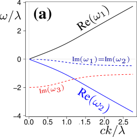
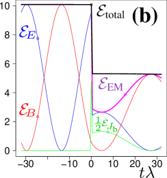
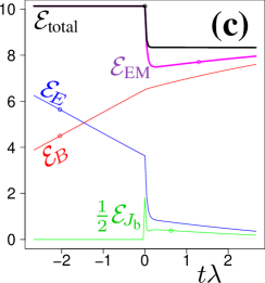
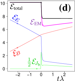
Figure 2: (a) The dispersion relation (28) for the simple material response model of (26), where $\chi_{{\scalebox{0.6}{0}}}=\epsilon_{{\scalebox{0.6}{0}}}\lambda$ and real $k$. The two propagating solutions $\omega_{1}$, $\omega_{2}\in{\mathbb{C}}$ have the same small damping, while the third $\omega_{3}\in\imath{\mathbb{R}}$ is pure loss. In (b,c,d) we see what happens as the system crosses a time boundary at $t=0$ between vacuum $\chi_{{\scalebox{0.6}{0}}}=0$ and $\chi_{{\scalebox{0.6}{0}}}=\epsilon_{{\scalebox{0.6}{0}}}\lambda$; where (c,d) show a narrower range of $t$ around $t=0$. The different initial conditions used in (b,c,d) demonstrate the timing-sensitive behaviour caused by the boundary. These graphs compare the energies in the three fields ${{\cal E}}_{\!E}=\epsilon_{{\scalebox{0.6}{0}}}E^{2}$, ${{\cal E}}_{\!B}=B^{2}/\mu_{{\scalebox{0.6}{0}}}$ and ${{\cal E}}_{\!J_{\text{b}}}=J_{\text{b}}^{2}/(\chi_{0}\lambda)$; but we show $\tfrac{1}{2}{{\cal E}}_{\!J_{\text{b}}}$ to increase visibility. Total energy is conserved for $t<0$; but just after the time boundary, ${{\cal E}}_{\!E}$ (and hence ${{\cal E}}_{\text{EM}}$) rapidly reduce as excitation is transferred to $J_{\text{b}}$, where it is strongly damped. The energy lost though $J_{\text{b}}$ depends on how strongly it is driven by $E$ until the new dynamic near-equilibrium is reached. Direct damping from the lossy $\omega_{3}$ solution is shown by the rapid and significant decay of ${{\cal E}}_{\!J_{\text{b}}}$ just after the transition.

VI Dynamic Material Models

It is not possible to both implement a physically consistent time boundary with a constant complex ${\epsilon_{{\textup{c}}}}$, and escape the requirement for the NBA in (25). This means we must instead use an explicitly causal [43] dynamic response model for the medium, thus providing fully dispersive CR. Since a response model adds extra field(s) to describe the material response, the coupled EM-material system will both have more than two modes and need ABCs. Essentially, defining a material response model immediately creates a demand for ABCs – they are simply the boundary conditions on the auxilliary fields (such as polarization ${\boldsymbol{P}}$ or bound current ${\boldsymbol{J}}_{\textup{b}}$) that one has decided to use.

A minimal but sufficient material response can be given by

$${\boldsymbol{D}}=\epsilon_{{\scalebox{0.6}{0}}}{\boldsymbol{E}}+{\boldsymbol{P}}\quad\textup{where}\quad\dot{{\boldsymbol{P}}}=-\lambda{\boldsymbol{P}}+\chi_{{\scalebox{0.6}{0}}}{\boldsymbol{E}},$$ (26)

so that in the steady state ${\boldsymbol{P}}=\chi_{{\scalebox{0.6}{0}}}\lambda^{-1}{\boldsymbol{E}}$. In this model, as long as the loss $\lambda$ is large compared to the field frequency, with the desired change in permittivity $\Delta\epsilon=\chi_{{\scalebox{0.6}{0}}}/\lambda$ held fixed, it indeed responds as if it were a medium of complex constant CR. This model also requires a boundary condition for the dielectric polarization ${\boldsymbol{P}}$ field, namely $[{\boldsymbol{P}}]=0$.

However, it is significant that the polarization field (26) is in fact derived from a bound current ${\boldsymbol{J}}_{\textup{b}}=\dot{\boldsymbol{P}}=-\lambda{\boldsymbol{P}}+\chi_{{\scalebox{0.6}{0}}}{\boldsymbol{E}}$. This ${\boldsymbol{J}}_{\textup{b}}$ is driven by, and hence indirectly applies loss to the field ${\boldsymbol{E}}$; and our simulation results shown in figure 2 use this ${\boldsymbol{J}}_{\textup{b}}$ approach. Used after the time boundary ($t>{{t_{{\textup{b}}}}}$), this medium has a dispersive behaviour given by

$${\widetilde{\epsilon}}(-\omega) =\epsilon_{{\scalebox{0.6}{0}}}+\frac{\chi_{{\scalebox{0.6}{0}}}}{\lambda-i\omega},$$ (27)

where $\chi_{{\scalebox{0.6}{0}}}>0$ and $\lambda>0$; and the steady state is reached when $\omega/\lambda\rightarrow 0$. The resulting cubic dispersion relation is

$$\epsilon_{{\scalebox{0.6}{0}}}\mu_{{\scalebox{0.6}{0}}}\left(\lambda-i\omega\right)\omega^{2}+\mu_{{\scalebox{0.6}{0}}}\chi_{{\scalebox{0.6}{0}}}\omega^{2}-k^{2}\left(\lambda-i\omega\right)=0.$$ (28)

This equation in $\omega$ and fixed $k^{2}$ produces three solutions as opposed to the two given in (11) or (24). Since (28) has real coefficients when written as a polynomial in $(i\omega)$, and as a cubic has at most two non-real roots for $i\omega$, the three solutions consist of a complex conjugate pair and a real valued one. The pair correspond to counter propagating waves (modes) with the same damping, with the other solution (mode) being non-propagating and purely damped (see figure 2(a)).

At a time boundary where $k\in{\mathbb{R}}$ and $k>0$, we have three outgoing modes, requiring three boundary conditions. Two TBC are given by either the natural (8) or fundamental (9) TBC (7); the ABC of course is just the $[{\boldsymbol{P}}]=0$ evident from the dynamic model (26). This ABC is analogous to the Pekar ABC [44], which are required when an EM wave passes into a spatially dispersive medium [45, 46].

Simulation results are shown in figure 2(b,c,d), demonstrating the system behaviour as it passes the boundary. Despite the excellent match to a medium with constant complex CR before and sufficiently far after the boundary transition, it does not exhibit the unphysical behaviour of prescribed constant complex CRs. Instead, just after $t=t_{b}=0$ in figures 2(c,d) we can see a rapid rebalancing as ${\boldsymbol{E}}$ and ${\boldsymbol{J}}_{\textup{b}}$ (i.e. $\dot{{\boldsymbol{P}}}$) adjust to the recently changed $\chi_{{\scalebox{0.6}{0}}}$.

Note also the overshoot in ${\cal E}_{J}$ just after the boundary, which can be attributed to the dampened $\omega_{3}$. These occur on a timescale set by $\lambda$, and incur an ${\boldsymbol{E}}$ dependent energy loss. From a dynamic perspective, system appears to have two loss processes, although both are in fact different manifestations of the same $\lambda$ loss term. In a steady-state medium, i.e. away from the boundary, the losses are gradual and proportional to $\omega/\lambda$. This counter-intuitive dependence on the $1/\lambda$ is because the loss depends on the mismatch between the ideal ${\boldsymbol{J}}_{\textup{b}}$ (or polarization ${\boldsymbol{P}}$) and the actual value; but for larger $\lambda$ values, the mismatch becomes smaller. In contrast, as the system transitions across the time boundary, the sudden change in $\chi_{{\scalebox{0.6}{0}}}$ means that the ${\boldsymbol{E}}$-dependent mismatch can suddenly become very large, and this causes equally large and rapid losses as ${\boldsymbol{J}}_{\textup{b}}$ (or ${\boldsymbol{P}}$) re-synchronise to the electric field ${\boldsymbol{E}}$. However, note that in the special case where ${\boldsymbol{E}}$ is zero at the boundary, the mismatch remains small and no significant rapid loss takes place.

A key further point of interest is whether there are any side-effects if the model parameters $\lambda$ and $\chi_{{\scalebox{0.6}{0}}}$ change with time. On the basis of (26) this does not appear to be the case, since the only time derivative term is that on the LHS, applied to ${\boldsymbol{P}}$. However, to check this properly we need to reformulate the model so that it is explicitly based on bound currents, which are the true microscopic physical property. Taking the time derivative of (26) and rearranging (see Appendix E) leads to the model equation

$$\dot{{\boldsymbol{K}}} =-\lambda\left[{\boldsymbol{K}}+\chi_{{\scalebox{0.6}{0}}}{\boldsymbol{E}}\right]~{}+~{}\frac{\dot{\lambda}}{\lambda}{\boldsymbol{K}},$$ (29)

where ${\boldsymbol{K}}={\boldsymbol{J}}_{\textup{b}}-\chi_{{\scalebox{0.6}{0}}}{\boldsymbol{E}}$ is an offset for the bound current ${\boldsymbol{J}}_{\textup{b}}$. This construction has ensured that there is only one time derivative applied to one field quantity (i.e. ${\boldsymbol{K}}$), so that it retains an unambiguously causal form [43]; it is in fact this equation we integrate, along with Maxwell’s equations, to get the results shown in Fig. 1(b-d) We can see from the equation that the value of ${\boldsymbol{K}}$ is going to be continually trying to catch up to the present value (albeit scaled) of ${\boldsymbol{E}}$, on a timescale set by $\lambda$. Since the introduction of ${\boldsymbol{K}}$ removes any dependence on the time derivative of $\chi_{{\scalebox{0.6}{0}}}$, a temporal boundary in the $\chi_{{\scalebox{0.6}{0}}}$ value is implemented simply by changing the parameter $\chi_{{\scalebox{0.6}{0}}}$ as we integrate step by step. However, extra care need to be taken if $\lambda$ changes at a temporal boundary; since its time derivative $\dot{\lambda}$ also appears. This would either be specified as part of the simulation environment defining $\chi_{{\scalebox{0.6}{0}}}$, $\lambda$, $\dot{\lambda}$; or we might add an auxilliary equation for $\lambda$ if it had its own temporal dynamics.

This model (i.e. (26), or (29)), being defined by a temporal differential equation, is necessarily explicitly causal [43]. It works as intended, i.e. to create a near-constant permittivity, when (i) the desired positive permittivity shift $\chi_{{\scalebox{0.6}{0}}}>0$, and when (ii) $\chi_{{\scalebox{0.6}{0}}}/\lambda\epsilon_{{\scalebox{0.6}{0}}}\lessapprox 3$. In this regime the polarization (or microscopic polarization current) adiabatically follows the phase of electric field, and so accurately models the desired effective permittivity; indeed the effective loss at low frequencies is proportional to $\omega/\lambda$, i.e. increasing the polarization current loss $\lambda$ actually reduces the effective damping in the CW limit. However, if the first condition does not hold, a positive polarization can have a negative energy; thus the amplitudes of ${\boldsymbol{E}}$ and ${\boldsymbol{P}}$ can increase without limit whilst still conserving energy. Alternatively, if the parameters change so that the second condition starts to fail, the three modes – two electromagnetic and one polarization – become ever more strongly coupled and eventually exhibit a complicated dynamics (and dispersion) not relevant to our presentation here.

VII Beyond the minimal dynamic model

The minimal model used above performs well, and has the considerable advantage of having a simple behaviour, thus clarifying the general principles for handling time boundaries. However, it is not typical of the material models used in practical situations which are often based on Drude or Lorentz oscillators that consider the polarization ${\boldsymbol{P}}$. Consequently, we now consider a more general situation by using the result that any causal response can be expressed as a sum of Lorentz responses [47]. Working in the time domain, we have ${\boldsymbol{D}}=\epsilon_{{\scalebox{0.6}{0}}}{\boldsymbol{E}}+\sum_{{s}}{\boldsymbol{P}}_{s}$. With ${s}_{\max}$ being the number of oscillators, we have then ${s}_{\max}$ second order equations:

$$\ddot{{\boldsymbol{P}}}_{s}+\left(\lambda_{s}{{\boldsymbol{P}}}_{s}\right)\dot{\,}+\alpha_{s}{\boldsymbol{P}}_{s}=\chi_{s}{\boldsymbol{E}}.$$ (30)

Here $\chi_{s}$ is the coupling, $\lambda_{s}$ is the damping, and $\alpha_{s}$ the natural frequency of the oscillator. Note that the time derivative in the second LH term acts on the product $\lambda_{s}{{\boldsymbol{P}}}_{s}$, not just on ${{\boldsymbol{P}}}_{s}$. Since the Lorentian oscillators follow second order dynamical equations, they will therefore each require two extra boundary conditions, for a total of $2{s}_{\max}$ ABCs. The natural ABCs for the ${s}$-th oscillator are

$$[{\boldsymbol{P}}_{s}]=0\qquad\textup{and}\qquad[2\dot{{\boldsymbol{P}}}_{s}+\lambda_{s}\,{\boldsymbol{P}}_{s}]=0.$$ (31)

To see this we substitute ${\boldsymbol{P}}(t,{\boldsymbol{x}})=\theta({{t_{{\textup{b}}}}}-t)\,{\boldsymbol{P}}_{s}^{\textup{a}}(t,{\boldsymbol{x}})+\theta(t-{{t_{{\textup{b}}}}})\,{\boldsymbol{P}}_{s}^{\textup{c}}(t,{\boldsymbol{x}})$ and likewise for $\lambda_{s}$, $\alpha_{s}$ and $\chi_{s}$, into (30) and assume (30) holds on both sides of the boundary. This gives

$$\delta^{\prime}({{t_{{\textup{b}}}}}-t)\,\big{(}{\boldsymbol{P}}_{s}^{\textup{c}}-{\boldsymbol{P}}_{s}^{\textup{a}}\big{)}+2\,\delta({{t_{{\textup{b}}}}}-t)\,\big{(}\dot{{\boldsymbol{P}}}_{s}^{\textup{c}}-\dot{{\boldsymbol{P}}}_{s}^{\textup{a}}\big{)}\qquad$$

$$+\delta({{t_{{\textup{b}}}}}-t)\,\big{(}\lambda_{s}^{\textup{c}}{{\boldsymbol{P}}}_{s}^{\textup{c}}-\lambda_{s}^{\textup{a}}{{\boldsymbol{P}}}_{s}^{\textup{a}}\big{)} =0.$$

The coefficients of $\delta^{\prime}({{t_{{\textup{b}}}}}-t)$ and $\delta({{t_{{\textup{b}}}}}-t)$ must both be zero. This gives (31). Observe that if $[\lambda_{s}]=0$ then (31) reduces to $[{\boldsymbol{P}}_{s}]=0$ and $[\dot{{\boldsymbol{P}}}_{s}]=0$. This result explains why in (30) that $\lambda_{s}$ is inside the time derivative in the second LH term. If it had been outside the derivative, then if $[{\boldsymbol{P}}_{s}]\neq 0$, the alternative $\lambda_{s}({{\boldsymbol{P}}}_{s})\dot{}$ would contain the product $\delta(t-{{t_{{\textup{b}}}}})\theta(t-{{t_{{\textup{b}}}}})$, which is not defined mathematically. An alternative method for setting out these ABCs would be to factorise (30) into two first order pieces; and it is also possible to follow either type of analysis for a bound current ${\boldsymbol{J}}_{\textup{b}}$ [48].

We can also calculate the number of ABCs required in the frequency domain, using the case of no boundary, or when the system is very far from the boundary. Here the parameters $\chi_{s}$, $\lambda_{s}$ can be treated as constants, where so that (30) gives us the dispersion

$${\widetilde{\epsilon}}(-\omega)=\epsilon_{{\scalebox{0.6}{0}}}+\sum_{{s}=1}^{{s}_{\max}}\frac{\chi_{s}}{-\omega^{2}-\imath\lambda_{s}\omega+\alpha_{s}^{2}}.$$ (32)

Expanding out the dispersion relation resulting from (2) then leads to a polynomial in $\omega$ of degree $(2{s}_{\max}+2)$, and hence $(2{s}_{\max}+2)$ modes. Matching these modes across a boundary between different materials will then require $(2{s}_{\max}+2)$ boundary conditions, $2{s}_{\max}$ of which are ABCs.

VIII Conclusion

We have shown that even simple time boundaries in optics cannot be described by the standard “constant complex permittivity” model. Only with a dynamic or dispersive model of the propagation medium can physical results be predicted. This conclusion is supported by NBA calculations and time domain simulations, and is easily generalized to other wave systems. It has significant implications for the design and modelling of both experiments and applications of future technologies based on temporal boundary phenomena. Our conclusion may be particularly relevant to the propagation of relativistically intense electromagnetic waves in plasma, the propagation of relativistic plasma waves in laser wakefield accelerators in the bubble regime, and for relativistic ionisation fronts and relativistically induced transparency in laser-solid interactions.

It is arguably unsurprising that a good model of a time boundary requires a model that can admit non-trivial time dependence, i.e. either a time domain response model or a frequency domain dispersion. Time boundaries are a temporal, dynamic phenomena, and need to be treated as such.

Appendix A In Linear Media – spatial evanescence

Lemma 1.

Given that for $\omega\in{\mathbb{R}}$, $\omega>0$ plane waves are spatially evanescent in the propagation direction then ${\textup{Im}}\big{(}{\widetilde{\epsilon}}(-\omega)\big{)}>0$.

Proof.

Given (1) with $\omega>0$. For ${\textup{Re}}(k)>0$ then the direction of propagation is positive $z$. If the plane waves are evanescent for positive $z$ then ${\textup{Re}}(ikz)<0$ hence ${\textup{Im}}(k)>0$. This implies $k$ lies in the top right quadrant of ${\mathbb{C}}$. Hence ${\textup{Im}}(k^{2})>0$.

Likewise for ${\textup{Re}}(k)<0$ then the direction of propagation is negative $z$. If the plane waves are evanescent for negative $z$ then ${\textup{Re}}(ikz)<0$ hence ${\textup{Im}}(k)<0$. This implies $k$ lies in the bottom left quadrant of ${\mathbb{C}}$. Hence ${\textup{Im}}(k^{2})>0$.

In both cases ${\textup{Im}}(k^{2})>0$ and since $\omega^{2}>0$ then (2) implies ${\textup{Im}}\big{(}{\widetilde{\epsilon}}(-\omega)\big{)}>0$. ∎

Appendix B In Linear Media – a note on negative refractive index

From (3), ${\textup{Im}}\left({\widetilde{\epsilon}}(-\omega)\right)>0$ implies that ${\tilde{{n}}}(-\omega)$ is either (a) in the top right quadrant of the complex plane ${\left\{{\textup{Re}}({\tilde{{n}}})>0\text{~{}and~{}}{\textup{Im}}({\tilde{{n}}})>0\right\}}$, or (b) in the bottom left quadrant ${\left\{{\textup{Re}}({\tilde{{n}}})<0\text{~{}and~{}}{\textup{Im}}({\tilde{{n}}})<0\right\}}$. Consequently, having ${\textup{Re}}\left({\tilde{{n}}}(-\omega)\right)<0$ does not contradict our assumption that the real part of both permittivity and permeability are positive: it is still possible to have a negative index of refraction [49, 50].

Appendix C Using a Narrowband Approximation – the eight roots

Demonstration of (19)-(22).

Since we chose (1) to satisfy (18) then this is (19) for $E_{x}=\exp({-i\omega t+ikz})$. Replacing $k\to=k$ then gives (19).

Replacing $\omega\to-\omega$ and $k\to-k$ then gives (21).

Taking the complex conjugate of (19) and using ${{\tilde{{n}}}({-{\overline{\omega}}})}={\overline{{\tilde{{n}}}({\omega})}}$ gives (22).

Replacing $\omega\to-\omega$ and $k\to-k$ in (22) then gives (21).

∎

Appendix D Using a Narrowband Approximation – proof

Proof of (24).

From (23) we have

$$B_{y}(t,z) =\frac{e^{k{C}_{\textup{I}}t}}{{C}_{\textup{I}}-i{C}_{\textup{R}}}\Big{(}{g^{-}_{+}}\,e^{-ik({C}_{\textup{R}}t-z)}-{g^{-}_{-}}\,e^{-ik({C}_{\textup{R}}t+z)}\Big{)}$$ (33)

$$\quad+\frac{e^{k{C}_{\textup{I}}t}}{{C}_{\textup{I}}+i{C}_{\textup{R}}}\Big{(}{g^{+}_{-}}\,e^{ik({C}_{\textup{R}}t-z)}-{g^{+}_{+}}\,e^{ik({C}_{\textup{R}}t+z)}\Big{)}$$

$$=\frac{{\overline{N}}\,e^{k{C}_{\textup{I}}t}}{{c_{{\scalebox{0.6}{0}}}}}\Big{(}{g^{-}_{+}}\,e^{-ik({C}_{\textup{R}}t-z)}-{g^{-}_{-}}\,e^{-ik({C}_{\textup{R}}t+z)}\Big{)}$$

$$\quad+\frac{N\,e^{k{C}_{\textup{I}}t}}{{c_{{\scalebox{0.6}{0}}}}}\Big{(}{g^{+}_{-}}\,e^{ik({C}_{\textup{R}}t-z)}-{g^{+}_{+}}\,e^{ik({C}_{\textup{R}}t+z)}\Big{)}$$

Using the fundamental TBC (9) we get for $t=0^{+}$ and $k\in{\mathbb{R}}$

$$E_{x}(0^{+},z) =e^{ikz}({g^{-}_{+}}+{g^{+}_{+}})+e^{-ikz}({g^{-}_{-}}+{g^{+}_{-}})$$

$${c_{{\scalebox{0.6}{0}}}}B_{y}(0^{+},z) =e^{ikz}({\overline{N}}{g^{-}_{+}}-N{g^{+}_{+}})+e^{-ikz}(N{g^{+}_{-}}-{\overline{N}}{g^{-}_{-}})$$

and hence

$${g^{-}_{+}}={\overline{{g^{+}_{-}}}}=\frac{E_{{\scalebox{0.6}{0}}}}{2}\frac{N+1}{N+{\overline{N}}}\quad\textup{and}\quad{g^{-}_{-}}={\overline{{g^{+}_{+}}}}=\frac{E_{{\scalebox{0.6}{0}}}}{2}\frac{{\overline{N}}+1}{N+{\overline{N}}}$$

Substituting into (23) gives (24). ∎

Appendix E The minimal model and bound currents

The concept behind our minimal model is that it should mimic the “ideal” of a constant-like permittivity with real and imaginary components. Thus we want there to exist a dielectric polarization ${\boldsymbol{P}}$ that closely follows the current value of the electric field ${\boldsymbol{E}}$, but allows freedom for dynamical variation about its chosen target value. Most simply, we can write

$$\partial_{t}{\boldsymbol{P}} =-\lambda{\boldsymbol{P}}+\chi_{{\scalebox{0.6}{0}}}{\boldsymbol{E}},$$ (34)

where in the steady-state limit we have the desired ${\boldsymbol{P}}=(\chi_{{\scalebox{0.6}{0}}}/\lambda){\boldsymbol{E}}=\Delta\varepsilon\,{\boldsymbol{E}}$. In this model, the dynamics are simply that ${\boldsymbol{P}}$ exponentially decays towards to $\Delta\varepsilon\,{\boldsymbol{E}}$ with rate $\lambda$.

However, from a microscopic point of view, a charge or current is the more useful physical property. Thus to adapt the initial concept in (34) we use the fact that ${\boldsymbol{J}}_{\textup{b}}=\partial_{t}{\boldsymbol{P}}$. However, since substitution of ${\boldsymbol{J}}_{\textup{b}}$ into (34) leaves us with no dynamics, we also apply an extra time derivative to the above equation. As a result we have

$$\partial_{t}{\boldsymbol{J}}_{\textup{b}} =-\lambda{\boldsymbol{J}}_{\textup{b}}+\partial_{t}\left(\chi_{{\scalebox{0.6}{0}}}{\boldsymbol{E}}\right)-\left(\partial_{t}\lambda\right){\boldsymbol{P}}.$$ (35)

Since this has time derivatives of fields on both sides, it is not straightforward to interpret it in a causal manner [43]. Thus we combine the ${\boldsymbol{J}}_{\textup{b}}$ and ${\boldsymbol{E}}$ fields, both of which are subject to an applied time derivative, into a single quantity:

$${\boldsymbol{K}} ={\boldsymbol{J}}_{\textup{b}}-\chi_{{\scalebox{0.6}{0}}}{\boldsymbol{E}}.$$ (36)

Thus we rearrange (35), and substitute for ${\boldsymbol{P}}$ using a rearranged (34), to get

$$\partial_{t}\left({\boldsymbol{J}}_{\textup{b}}-\chi_{{\scalebox{0.6}{0}}}{\boldsymbol{E}}\right) =-\lambda{\boldsymbol{J}}_{\textup{b}}~{}-~{}\left(\partial_{t}\lambda\right)\frac{1}{\lambda}\left[\chi_{{\scalebox{0.6}{0}}}{\boldsymbol{E}}-\partial_{t}{\boldsymbol{P}}\right],$$ (37)

$$\partial_{t}{\boldsymbol{K}} =-\lambda{\boldsymbol{J}}_{\textup{b}}~{}+~{}\left(\partial_{t}\lambda\right)\frac{1}{\lambda}\left[{\boldsymbol{J}}_{\textup{b}}-\chi_{{\scalebox{0.6}{0}}}{\boldsymbol{E}}\right],$$ (38)

$$\partial_{t}{\boldsymbol{K}} =-\lambda\left[{\boldsymbol{K}}+\chi_{{\scalebox{0.6}{0}}}{\boldsymbol{E}}\right]~{}+~{}\frac{\partial_{t}\lambda}{\lambda}{\boldsymbol{K}}.$$ (39)

where the changes (effects) on the LHS from the first RHS term are determined solely by the known present values of ${\boldsymbol{K}}$ and ${\boldsymbol{E}}$. If the system parameter $\lambda$ is time dependent (i.e. $\lambda(t)$), then see also that we need to know $\partial_{t}\lambda$ as well as $\lambda$; although such a specification is not required for $\chi_{{\scalebox{0.6}{0}}}$. This is particularly relevant in the case of an (otherwise constant) medium with an abrupt change at a time boundary.

From (39) we can see that the value of ${\boldsymbol{K}}$ is going to be continually trying to catch up to the present value (albeit scaled) of ${\boldsymbol{E}}$, on a timescale set by $\lambda$. Clearly, for this model to function as intended we will want the $\lambda$ timescale to be faster than the largest significant frequency component of ${\boldsymbol{E}}$.

In the harmonic case, we can Fourier transform the evolution equation; here a time-domain field $A(t)$ becomes a frequency-domain $\tilde{A}(\omega)$. Then (39) tells us that

$$-\imath\omega\tilde{{\boldsymbol{K}}} =-\lambda\left(\tilde{{\boldsymbol{K}}}+\chi_{{\scalebox{0.6}{0}}}\tilde{{\boldsymbol{E}}}\right),$$ (40)

$$\textrm{i.e.}\qquad\tilde{{\boldsymbol{K}}} =\frac{-\chi_{{\scalebox{0.6}{0}}}\lambda}{-\imath\omega+\lambda}\tilde{{\boldsymbol{E}}}\qquad\textrm{or}\qquad\tilde{{\boldsymbol{J}}_{\textup{b}}}=\chi_{{\scalebox{0.6}{0}}}\left[\frac{-\lambda}{\lambda-\imath\omega}+1\right]\tilde{{\boldsymbol{E}}}.$$ (41)

In the intended limit where $\lambda\gg\omega$, we can expand to second order so that

$$\tilde{{\boldsymbol{J}}_{\textup{b}}} \simeq-\imath\omega\chi_{{\scalebox{0.6}{0}}}\lambda^{-1}\left[1-\imath\omega\lambda^{-1}\right]\tilde{{\boldsymbol{E}}},$$ (42)

and as a result we have  

$$\tilde{{\boldsymbol{P}}} =\left[\Delta\varepsilon_{r}-\imath\Delta\varepsilon_{i}(\omega)\right]\tilde{{\boldsymbol{E}}},\qquad\textrm{where}\qquad\Delta\varepsilon_{i}(\omega)=\Delta\varepsilon_{r}\omega/\lambda.$$ (43)

This means that this minimal dynamical model for the standard “constant permittivity” assumption which will match the target real-valued permittivity in the large $\lambda$ limit, with the concommitant introduction of a loss that gets ever smaller in the ideal large $\lambda$ limit.

Appendix F Remarks – Causality, dispersion, and the NBA

Across our time boundary, a change in constant complex CR for a medium is just an instantaneous change, which is straightforwardly causal. Causal behaviour, however, of itself is not necessarily guaranteed to give physically reasonable predictions. Indeed, all but one of the results in this paper are causal – even the unphysical (17), where the future behaviour is by construction explicitly dependent on the past behaviour. The single exception is the narrowband result (25), because under this approximation questions of causality are moot.

Causality is often tested by applying the Kramers-Kronig relations (see e.g. [43]), but they do not apply to all situations. For example, even though the result (16) is causal, and clearly so when solving in the time domain, as an exponentially increasing function it cannot be Fourier transformed so as to allow Kramers-Kronig to be tested. Indeed, since the original function of Kramers-Kronig was to analyse, test, or correct raw data collected in the frequency domain, using them as a causality test when a time domain description is already available is redundant.

This is why the dynamical model (26) is a natural starting point for an examination of temporal boundaries; although of course more complicated models, such as the summed Lorentzians of (32), or ones involving (causal) integral kernels, can be constructed. Notably, even the highly simplified (26), designed to give results that in the appropriate limit are as close as possible to the failed constant complex CR model, is sufficient to restore physical behaviour.

Appendix G Material responses: Cauchy and convolutions

In principle, we could try to expressed this time boundary situation as a Cauchy problem – i.e. namely asking what is the subsequent wave behaviour if the Cauchy (initial condition) data is $E(z)=E_{0}\cos(k_{a}z)$. However, it is not clear how this extended field could be set up as a realistic initial condition; and, further, trying to use a straightforward convolution approach would fail because $E(z,t)$ for $t<0$ (i.e. the pre-boundary field) would be unknown.

For convolution transforms, we note that their standard use in constitutive relations is of the time-independent form $D(t)=\int\epsilon(t-t^{\prime})E(t^{\prime})dt^{\prime}$, but unfortunately, this would only be valid – obviously – for time independent media. For time dependent media, such as one including a time boundary, we would need to use the two-time generalisation $D(t)=\int\epsilon(t,t^{\prime})E(t^{\prime})dt^{\prime}$.

Whilst in principle such generalisations can be written down, it is unfortunate that the time-independent convolution does not indicate in any way how a general (two-time) formulation could be arrived at, and this is complicated further since the convolution include the time boundary itself. This is in stark contrast to dynamic response models such as (26), or the more general form given here in the appendix as (32), where insisting on (e.g.) continuity of the auxiliary fields is quite natural.

Appendix H Remarks – CR and Ohmic losses

Ohmic losses are also covered by our analysis; as they can also be modelled by a complex permittivity. Since the polarisation corresponding to ohmic losses is given by ${\boldsymbol{P}}=(\sigma/(-i\omega)){\boldsymbol{E}}$ then this is an alternative dispersive constitutive relation, which means it does not contradict the statements about constant ${\epsilon_{{\textup{c}}}}$.