Waste-free sequential Monte Carlo

Abstract.

A standard way to move particles in an SMC sampler is to apply several steps of an MCMC (Markov chain Monte Carlo) kernel. Unfortunately, it is not clear how many steps need to be performed for optimal performance. In addition, the output of the intermediate steps are discarded and thus wasted somehow. We propose a new, waste-free SMC algorithm which uses the outputs of all these intermediate MCMC steps as particles. We establish that its output is consistent and asymptotically normal. We use the expression of the asymptotic variance to develop various insights on how to implement the algorithm in practice. We develop in particular a method to estimate, from a single run of the algorithm, the asymptotic variance of any particle estimate. We show empirically, through a range of numerical examples, that waste-free SMC tends to outperform standard SMC samplers, and especially so in situations where the mixing of the considered MCMC kernels decreases across iterations (as in tempering or rare event problems).

1. Introduction

1.1. Background

Sequential Monte Carlo (SMC) methods are iterative stochastic algorithms that approximate a sequence of probability distributions through successive importance sampling, resampling, and Markov steps. Historically, they were mainly used to approximate the filtering distributions of a state-space model. More recently, they have been extended to an arbitrary sequence of probability distributions (Neal,, 2001; Chopin,, 2002; Del Moral et al.,, 2006); in such applications, they are often called “SMC samplers”.

As an illustrative example, consider the tempering sequence:

(1) $$\pi_{t}(\mathrm{d}x)\propto\nu(\mathrm{d}x)L(x)^{\gamma_{t}}$$

based on increasing exponents, $0=\gamma_{0}<\ldots<\gamma_{T}=1$. This sequence may be used to interpolate between a distribution $\nu(\mathrm{d}x)$, which is easy to sample from, and a distribution of interest, $\pi(\mathrm{d}x)\propto\nu(\mathrm{d}x)L(x)$ (e.g. a Bayesian posterior distribution), which may be difficult to simulate directly. Other sequences of interest will be discussed later.

When used to sample from a fixed distribution (as in tempering), SMC samplers present several advantages over MCMC (Markov chain Monte Carlo). First, they provide an estimate of the normalising constant of the target distribution at no extra cost; this quantity is of interest in several cases, in particular in Bayesian model choice (e.g. Zhou et al.,, 2016). Second, they are easy to parallelise, as the bulk of the computation treats the $N$ particles independently (Lee et al.,, 2010). Third, it is easy to make SMC samplers “adaptive”; that is, to use the current particle sample to automate the choice of most of its tuning parameters. This is often crucial for good performance.

To elaborate on the third point, a common strategy to move the particles is to apply a $k-$fold MCMC kernel that leaves the current distribution $\pi_{t}$ invariant. One may use for instance a random walk Metropolis kernel, with the covariance of the proposal set to a small multiple of the empirical covariance of the particle sample. In that way, the algorithm automatically scales to the current distribution.

However, one tuning parameter of SMC samplers that is often overlooked in the literature is the number $k$ of MCMC steps that should be applied to move the particles. For instance, Chopin and Ridgway, (2017) set $k=3$ arbitrarily in their numerical experiments, but it turns out that this value is very sub-optimal, as we show in our first numerical example.

A second issue with $k$ is that there is no reason to set it to a fixed value across iterations. In application such as tempering, $\pi_{t}$ may become more and more difficult to explore through MCMC; thus $k$ should be increased accordingly, and may become very large.

To deal with these two issues, one could set $k$ adaptively; that is, iterate MCMC steps until a certain stability criterion is met (Drovandi and Pettitt,, 2011; Kantas et al.,, 2014; Ridgway,, 2016; Salomone et al.,, 2018; Buchholz et al.,, 2020). However, in our experience, these approaches are not always entirely reliable. There seems to be a fundamental difficulty in determining, after $k$ steps have been performed, that this value of $k$ is optimal, without performing several extra steps.

A third, and perhaps more essential issue, is that, if indeed large values of $k$ are required for good performance, the intermediate output of these $k$ MCMC steps are not used directly, and seems somehow wasted.

1.2. Motivation and plan

These issues motivated us to develop a waste-free SMC algorithm that exploits the intermediate outputs of these MCMC steps; see Section 2. The basic idea is to resample only $M=N/P$ out of the $N$ previous particles, for some $P\geq 2$. Then each resampled particle is moved $P-1$ times through the chosen MCMC kernel. The resampled particles and their $P-1$ iterates are gathered to form a new sample of size $N$.

Standard results on the convergence of SMC estimates cannot be applied directly to this new algorithm. We were able nonetheless to establish the consistency and asymptotic normality of the output of waste-free SMC; see Section 3. We also compared the performance and the robustness of waste-free SMC and standard SMC through an artificial example.

These theoretical results (in particular the expression of the asymptotic variance) gives us various insights on how to implement waste-free SMC in practice; see Section 4. In particular, we are able to derive variance estimates and confidence intervals for any particle estimate, which may be computed from a single run.

To assess the performance and versatility of waste-free SMC, we perform numerical experiments in three different scenarios where SMC samplers already give state-of-the-art performance: logistic regression with a large number of predictors; the enumeration of Latin squares; and the computation of Gaussian orthant probabilities; see Section 5. In each case, waste-free SMC performs at least as well as properly tuned SMC samplers, while requiring considerably less tuning effort.

Proofs are delegated to the appendix.

1.3. Related work

We focus on SMC samplers based on invariant (MCMC) kernels. These algorithms have proved popular recently in a variety of applications, such as rare events (Johansen et al.,, 2006; Cérou et al.,, 2012); experimental designs (Amzal et al.,, 2006); cross-validation (Bornn et al.,, 2010); variable selection (Schäfer and Chopin,, 2013); graphical models (Naesseth et al.,, 2014); PAC-Bayesian classification (Ridgway et al.,, 2014); Gaussian orthant probabilities (Ridgway,, 2016); Bayesian model choice in hidden Markov models (Zhou et al.,, 2016), and un-normalised models (Everitt et al.,, 2017); among others.

We note in passing that SMC samplers may be generalised to non-invariant kernels, as shown in Del Moral et al., (2006); see also Heng et al., (2020) for how to calibrate such kernels. On the other hand, it is also possible to add MCMC steps to various SMC algorithms that are not SMC samplers; the idea goes back to Berzuini et al., (1997). In particular, SMCMC (Sequential MCMC, Septier et al.,, 2009; Septier and Peters,, 2016; Finke et al.,, 2020) algorithms approximate recursively the filtering distribution of a state-space model: each iteration $t$ runs a MCMC chain that leaves invariant a certain (partly discrete) approximation of the current filter. It is not clear however how to derive a waste-free version of these algorithms, and thus we do not consider them further.

Finally, we mention that several improvements proposed for standard SMC samplers might be also adapted to waste-free SMC, such as methods to combine the output of the intermediate steps, see Beskos et al., (2017) and South et al., (2019).

Tan, (2015) proposes several algorithms that are variations of the resample-move algorithm of Gilks and Berzuini, (2001); one of them (generalized resample-move) bears a similarity with waste-free SMC in the context of of tempering.

2. Proposed algorithm

2.1. Notations

Throughout the paper, $(\mathcal{X},\mathbb{X})$ stands for a measurable space, and $\varphi:\mathcal{X}\rightarrow\mathbb{R}$ for a measurable function; let $\left\lVert\varphi\right\rVert_{\infty}:=\sup_{x\in\mathcal{X}}|\varphi(x)|$ (supremum norm). The expectation of $\varphi(X)$ when $X\sim\pi(\mathrm{d}x)$ is denoted by $\pi(\varphi)$; i.e. $\pi(\varphi):=\int\varphi(x)\pi(\mathrm{d}x)$. Recall that a Markov kernel $K(x,\mathrm{d}y)$ is a map $K:\mathcal{X}\times\mathbb{X}\rightarrow[0,1]$ such that $x\rightarrow K(x,A)$ is measurable in $x$, for any $A\in\mathbb{X}$; and $A\rightarrow K(x,A)$ is a probability measure (on $(\mathcal{X},\mathbb{X})$), for any $x\in\mathcal{X}$. We use the following standard notations for the integral operators associated to Markov kernel $K$: $\pi K$ is the distribution such that $\pi K(A)=\int_{\mathcal{X}}\pi(\mathrm{d}x)K(x,A)$, and $K(\varphi)$ is the function $x\rightarrow\int_{\mathcal{X}}K(x,\mathrm{d}y)\varphi(y)$, for $\varphi:\mathcal{X}\rightarrow\mathbb{R}$.

Symbol $\Rightarrow$ means convergence in distribution, and $\left\lVert\cdot\right\rVert_{\operatorname{TV}}$ stands for the total variation norm, $\left\lVert\mu-\nu\right\rVert_{\operatorname{TV}}=\sup_{A\in\mathbb{X}}|\mu(A)-\nu(A)|$.

2.2. A generic SMC sampler

We consider a generic sequence of target probability distributions of the form (for $t=0,1,\ldots,T$):

(2) $$\pi_{t}(\mathrm{d}x)=\frac{1}{L_{t}}\gamma_{t}(x)\nu(\mathrm{d}x)$$

where $\nu(\mathrm{d}x)$ is a probability measure, with respect to measurable space $(\mathcal{X},\mathbb{X})$, $\gamma_{t}$ is a measurable, non-negative function, and $L_{t}:=\int_{\mathcal{X}}\gamma_{t}(x)\nu(\mathrm{d}x)$, the normalising constant, is assumed to be properly defined, i.e. $0<L_{t}<\infty$. In the tempering scenario mentioned in the introduction, $\gamma_{t}(x)=L(x)^{\gamma_{t}}$, for certain exponents $\gamma_{t}$. Other interesting scenarios include data tempering (sequential learning), where $x$ represents a parameter, $\nu(\mathrm{d}x)$ its prior distribution, and $\gamma_{t}(x)$ is the likelihood of data-points $y_{0},\ldots,y_{t}$; rare-event simulation (and likelihood-free inference), where $\gamma_{t}(x)=\mathbb{1}_{\mathcal{E}_{t}}(x)$, the indicator function of nested sets $\mathcal{E}_{0}\supset\mathcal{E}_{1}\supset\ldots$; among others. See e.g. Chapter 3 of Chopin and Papaspiliopoulos, (2020) for a review of common applications of SMC samplers, and the sequence of target distributions arising in these applications.

One way to track the sequence $\pi_{t}$ would be to perform sequential importance sampling: sample particles (random variates) from the initial distribution $\nu(\mathrm{d}x)$, then reweight them sequentially according to weight function $G_{t}(x):=\gamma_{t}(x)/\gamma_{t-1}(x)$ (for $t\geq 1$, and $G_{0}(x):=\gamma_{0}(x)$). In most applications however, the weights degenerate quickly, making this naive approach useless.

SMC samplers alternate such reweighting steps with resampling and Markov steps. For the latter, we introduce Markov kernels $M_{t}(x_{t-1},\mathrm{d}x_{t})$ which leave invariant the target distributions: $\pi_{t-1}M_{t}=\pi_{t-1}$ for $t\geq 1$. It is easy to check that the sequence of Feynman-Kac distributions (for $t=0,\ldots,T$) defined as:

(3) $$\mathbb{Q}_{t}(\mathrm{d}x_{0:t})=\frac{1}{L_{t}}\nu(\mathrm{d}x_{0})\prod_{s=1}^{t}M_{s}(x_{s-1},\mathrm{d}x_{s})\prod_{s=0}^{t}G_{s}(x_{s})$$

is such that the marginal distribution of variable $X_{t}$ (with respect to $\mathbb{Q}_{t}$) is $\pi_{t}$. We call Feynman-Kac model the set of the components that define this sequence of distributions, that is, the initial distribution $\nu$, the kernels $M_{t}$, $t=1,\ldots,T$, and the functions $G_{t}$, $t=0,\ldots,T$. For more background on Feynman-Kac distributions, see e.g. Del Moral, (2004).

Algorithm 1 recalls the structure of an SMC sampler that corresponds to this Feynman-Kac model; and in particular which targets at each iteration $t$ distribution $\pi_{t}$. It takes as inputs: $N$, the number of particles, the considered Feynman-Kac model, and the chosen resampling scheme (function resample). Several resampling schemes exist. In this paper, we focus for simplicity on multinomial resampling, which generates ancestor variables $A_{t}^{n}$ independently from the categorical distribution that generates label $m$ with probability $W_{t}^{m}$.

Input: Integer $N\geq 1$, a Feynman-Kac model (initial distribution $\nu(\mathrm{d}x)$, functions $G_{t}$, Markov kernels $M_{t}$)

for $t\leftarrow 0$ to $T$ do

       if $t=0$ then

             for $n=1$ to $N$ do

                   $X_{0}^{n}\sim\nu(\mathrm{d}x_{0})$

            

      else

             $A_{t}^{1:N}\sim\textnormal{{resample}}(N,W_{t-1}^{1:N})$

             for $n=1$ to $N$ do

                   $X_{t}^{n}\sim M_{t}(X_{t-1}^{A_{t}^{n}},\mathrm{d}x_{t})$

                  

            

      for $n\leftarrow 1$ to $N$ do

            $w_{t}^{n}\leftarrow G_{t}(X_{t}^{n})$

            

      for $n\leftarrow 1$ to $N$ do

             $W_{t}^{n}\leftarrow w_{t}^{n}/\sum_{m=1}^{N}w_{t}^{m}$

            

      

Algorithm 1 Generic SMC sampler

At any iteration $t$, quantity $\sum_{n=1}^{N}W_{t}^{n}\varphi(X_{t}^{n})$ is an estimate of the expectation $\pi_{t}(\varphi)$, for $\varphi:\mathcal{X}\rightarrow\mathbb{R}$, and quantity $L_{t}^{N}:=\prod_{s=0}^{t}\ell_{s}^{N}$, where $\ell_{s}^{N}:=N^{-1}\sum_{n=1}^{N}w_{s}^{n}$, is an estimate of the normalising constant $L_{t}$. These estimates are consistent and asymptotically normal (as $N\rightarrow+\infty$) under general conditions.

2.3. Note on the generality of Algorithm 1

While generic, Algorithm 1 is a simplified version of most practical SMC samplers. In particular, we have stressed in the introduction the importance of making SMC samplers adaptive; that is, to adapt both the distributions $\pi_{t}$ and the Markov kernels $M_{t}$ on the fly. This means that these quantities may depend on the current particle sample. For simplicity, our notations do not account for this. We will see later that similar adaptation tricks may be developed for waste-free SMC.

Another interesting generalisation is when the state space $\mathcal{X}$ evolves over time; in particular when its dimension increases. This happens for instance when performing sequential inference on a model involving latent variables. The ideas developed in this paper may easily be adapted to this scenario, as we shall see in our third numerical example. For the sake of exposition, however, we focus on the fixed state space case.

2.4. Proposed algorithm: waste-free SMC

The idea behind waste-free SMC is to resample only $M$ ancestors, with $M\ll N$. Then each of these ancestors is moved $P-1$ times through Markov kernel $M_{t}$. The resulting $M$ chains of length $P$ are then put together to form a new particle sample, of size $N=MP$. See Algorithm 2.

Input: Integers $M,P\geq 1$ (let $N\leftarrow MP$), a Feynman-Kac model (initial distribution $\nu(\mathrm{d}x)$, functions $G_{t}$, Markov kernels $M_{t}$)

for $t\leftarrow 0$ to $T$ do

       if $t=0$ then

             for $n\leftarrow 1$ to $N$ do

                   $X_{0}^{n}\sim\nu(\mathrm{d}x_{0})$

                  

            

      else

             $A_{t}^{1:M}\sim\textnormal{{resample}}(M,W_{t-1}^{1:N})$

             for $m\leftarrow 1$ to $M$ do

                   $\tilde{X}_{t}^{m,1}\leftarrow X_{t-1}^{A_{t}^{m}}$

                   for $p\leftarrow 2$ to $P$ do

                         $\tilde{X}_{t}^{m,p}\leftarrow M_{t}(\tilde{X}_{t}^{m,p-1},\mathrm{d}x_{t})$

                        

                  

            Gather variables $\tilde{X}_{t}^{m,p}$ so as to form new sample $X_{t}^{1:N}$

            

      for $n\leftarrow 1$ to $N$ do

             $w_{t}^{n}\leftarrow G_{t}(X_{t}^{n})$

            

      for $n\leftarrow 1$ to $N$ do

             $W_{t}^{n}\leftarrow w_{t}^{n}/\sum_{m=1}^{N}w_{t}^{m}$

            

      

Algorithm 2 Waste-free SMC sampler

The output of the algorithm may be used exactly in the same way as for standard SMC: e.g. $\sum_{n=1}^{N}W_{t}^{n}\varphi(X_{t}^{n})$ is an estimate of $\pi_{t}(\varphi)$.

To get some intuition why waste-free SMC may be a valid and interesting alternative to standard SMC, consider at time $t-1$ a fictitious particle $X_{t-1}^{n}$, whose weight $W_{t-1}^{n}$ is large. In a standard SMC sampler, this particle is selected many times as an ancestor for the Markov step. Then, if $M_{t}$ mixes poorly, its many children will be strongly correlated.

On the other hand, in waste-less SMC, provided that $M\ll N$, the particle $X_{t-1}^{n}$ is selected a much smaller number of times; each time it is selected, $P$ successive variables are introduced in the sample. By construction, two such variables should be less correlated than if they had the same ancestor (as in standard SMC); see Figure 1 for a graphical representation of this idea.

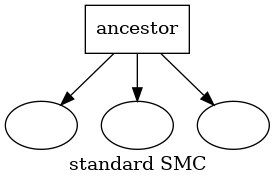
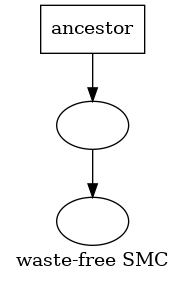
Figure 1. Pictorial representation of dependencies in standard SMC and waste-free SMC. Left: in standard SMC, an ancestor generates $3$ children for the next iteration. Right: in waste-free SMC, the same ancestor generates itself, one child, and one grand-child. Each arrow corresponds to one transition through kernel $M_{t}$.

Another insight is provided by chaos propagation theory (Del Moral,, 2004, Chap. 8), which says that, when $M\ll N$, $M$ resampled particles behave essentially like $M$ independent variables that follows the current target distribution. Thus, in a certain asymptotic regime, we expect the particle sample to behave like the variables of $M$ independent, stationary Markov chains, of length $P$.

Before backing these intuitions with a proper analysis, we provide a last insight regarding the underlying structure of waste-free SMC.

2.5. Feynman-Kac model associated with waste-free SMC

Algorithm 2 may be cast as a standard SMC sampler that propagates and reweights particles that are Markov chains of length $P$. The components of the corresponding Feynman-Kac model may be defined as follows. Assume $P\geq 1$ is fixed. Let $\mathcal{Z}=\mathcal{X}^{P}$, and, for $z\in\mathcal{Z}$, denote component $p$ as $z[p]$: $z=(z[1],\ldots,z[P])$. Then define the potential functions as:

(4) $$G_{t}^{\mathrm{wf}}(z):=\frac{1}{P}\sum_{p=1}^{P}G_{t}(z[p])$$

the initial distribution as: $\nu^{\mathrm{wf}}(\mathrm{d}z):=\prod_{p=1}^{P}\nu(\mathrm{d}z[p])$, and the Markov kernels as:

(5) $$M_{t}^{\mathrm{wf}}(z_{t-1},\mathrm{d}z_{t}):=\\ \left\{\sum_{p=1}^{P}\frac{G_{t-1}(z_{t-1}[p])}{\sum_{q=1}^{P}G_{t-1}(z_{t-1}[q])}\times M_{t}(z_{t-1}[p],\mathrm{d}z_{t}[1])\right\}\prod_{p=2}^{P}M_{t}(z_{t}[p-1],\mathrm{d}z_{t}[p]).$$

The following proposition explains how this waste-free Feynman-Kac model relates to the initial Feynman-Kac model of Algorithm 1.

Proposition 1.

The Feynman-Kac model associated with initial distribution $\nu^{\mathrm{wf}}$, Markov kernels $M_{t}^{\mathrm{wf}}$, and functions $G_{t}^{\mathrm{wf}}$, that is, the sequence of distributions:

$$\mathbb{Q}_{t}^{\mathrm{wf}}(dz_{0:t})=\frac{1}{L_{t}^{\mathrm{wf}}}\nu^{\mathrm{wf}}(\mathrm{d}z_{0})\prod_{s=1}^{t}M_{s}^{\mathrm{wf}}(z_{s-1},\mathrm{d}z_{s})\prod_{s=0}^{t}G_{s}^{\mathrm{wf}}(z_{s})$$

where $L_{t}^{\mathrm{wf}}$ is a normalising constant, is such that:

• $L_{t}^{\mathrm{wf}}=L_{t}$, the normalising constant of (2) and (3);

• $\mathbb{Q}_{t}^{\mathrm{wf}}(dz_{t})$ is the distribution of a stationary Markov chain of size $P$ whose Markov kernel is $M_{t}$ (and thus whose initial distribution is $\pi_{t}$):

  $$\mathbb{Q}_{t}^{\mathrm{wf}}(\mathrm{d}z_{t})=\pi_{t}(\mathrm{d}z_{t}[1])\prod_{p=2}^{P}M_{t}(z_{t}[p-1],\mathrm{d}z_{t}[p]).$$

We can now interpret Algorithm 2 as an instance of Algorithm 1 where the number of particles is $M$, and the underlying Feynman-Kac model is defined as above. In particular, consider how Algorithm 1 would operate if applied to that Feynman-Kac model. At time $t$, it would select randomly an ancestor $z_{t-1}$ (a chain of length $P$), with probability $\propto\sum_{p=1}^{P}G_{t-1}(z_{t-1}[p])$. Then, when kernel $M_{t}^{\mathrm{wf}}$ is applied to this chain, one component would be selected randomly, with probability $G_{t-1}(z_{t-1}[p])/\sum_{q=1}^{P}G_{t-1}(z_{t-1}[q])$. Thus, this particular component would be used as a starting point of the subsequent chain with probability $\propto G_{t-1}(z_{t-1}[p])$. This is precisely what is done in Algorithm 2.

This interpretation of waste-free SMC as a standard SMC sampler makes it easy to derive several of its properties; for instance, regarding its estimates of the normalising constants.

Proposition 2.

At iteration $t\geq 0$ of Algorithm 2 , the quantity

(6) $$L_{t}^{N}:=\prod_{s=0}^{t}\ell_{s}^{N},\quad\mbox{where }\ell_{s}^{N}:=\frac{1}{N}\sum_{n=1}^{N}G_{s}(X_{s}^{n})$$

is an unbiased estimate of $L_{t}$, the normalising constant of target distribution $\pi_{t}$, as defined in (2).

This proposition is a small variation over the well known result of (Del Moral,, 1996) that, in a standard SMC sampler, the estimate of the normalising constant estimate is unbiased.

We can also use the interpretation of waste-free SMC as a standard SMC sampler to derive asymptotic results.

Proposition 3.

For $P\geq 1$ fixed, and $\varphi:\mathcal{X}\rightarrow\mathbb{R}$ measurable and bounded, the output of Algorithm 2 at time $t\geq 0$ is such that

(7) $$\sqrt{N}\left(\frac{1}{N}\sum_{n=1}^{N}\varphi(X_{t}^{n})-\pi_{t-1}(\varphi)\right) \Rightarrow\mathcal{N}\left(0,\tilde{\mathcal{V}}_{t}^{P}(\varphi)\right)$$

(8) $$\sqrt{N}\left(\sum_{n=1}^{N}W_{t}^{n}\varphi(X_{t}^{n})-\pi_{t}(\varphi)\right) \Rightarrow\mathcal{N}\left(0,\mathcal{V}_{t}^{P}(\varphi)\right)$$

as $M\rightarrow+\infty$, $N=MP$, where $\pi_{t-1}$ means $\nu$ in (7) when $t=0$, $\tilde{\mathcal{V}}_{0}^{P}(\varphi):=\mathrm{Var}_{\nu}(\varphi)$,

(9) $$\tilde{\mathcal{V}}_{t}^{P}(\varphi) :=\mathcal{V}_{t-1}^{P}(\bar{M}_{t}^{P}\varphi)+v_{P}(M_{t},\varphi),\quad t\geq 1,$$

(10) $$\mathcal{V}_{t}^{P}(\varphi) :=\tilde{\mathcal{V}}_{t}^{P}\left(\bar{G_{t}}(\varphi-\pi_{t}\varphi)\right),\quad t\geq 0,$$

$\bar{G}_{t}:=G_{t}/\ell_{t}$, $\bar{M}_{t}^{P}=P^{-1}\sum_{p=1}^{P}M_{t}^{p-1}$,

$$v_{P}(M_{t},\varphi):=\mathrm{Var}\left(\frac{1}{\sqrt{P}}\sum_{p=0}^{P-1}\varphi(Y_{p})\right)$$

and $(Y_{p})_{p\geq 0}$ stands for a stationary Markov chain with kernel $M_{t}$ (i.e. $Y_{0}\sim\pi_{t}$).

This proposition is stated without proof, as it amounts to applying known central limit theorems (see Chapter 11 of Chopin and Papaspiliopoulos,, 2020, and references therein) for SMC estimates to the waste-free Feynman-Kac model mentioned above. Notice how the asymptotic variances depend on $P$ in a non-trivial way. This suggests that the fixed $P$ regime is not very convenient; in particular it is not clear how to choose $P$ for optimal performance. If we take $P\rightarrow+\infty$, we expect the first term of (9) to go to zero, and the second term to converge to the asymptotic variance of kernel $M_{t}$. This suggests, at the very least, that taking $P$ large may often be reasonable. The next section studies the asymptotic behaviour of the algorithm as $P\rightarrow+\infty$.

3. Convergence as $P\rightarrow+\infty$

3.1. Assumptions

This section is concerned with the behaviour of waste-free SMC in the “long-chain” regime, that is, when $P\rightarrow+\infty$, while $M$ is either fixed or may grow with $P$ at some rate. We start by remarking that this regime requires some assumption on the mixing of the Markov kernels $M_{t}$. Indeed, assume that $M_{t}$ is the identity kernel: $M_{t}(x_{t-1},\mathrm{d}x_{t})=\delta_{x_{t-1}}(\mathrm{d}x_{t})$. In that case, at time $1$, one has:

$$\frac{1}{N}\sum_{n=1}^{N}\varphi(X_{1}^{n})=\frac{1}{M}\sum_{m=1}^{M}\varphi(X_{0}^{A_{0}^{m}})$$

since the $P$ particles $\tilde{X}_{t}^{m,p}$ are identical for a given $m$. The variance of this quantity should be $\mathcal{O}(M^{-1})$, and cannot go to zero if $M$ is kept fixed.

We thus consider the following assumptions.

Assumption (M).

The Markov kernels $M_{t}$ are uniformly ergodic, that is, there exist constants $C_{t}\geq 0$ and $\rho_{t}\in[0,1[$ such that,

$$\left\lVert M_{t}^{k}(x_{t-1},\mathrm{d}x_{t})-\pi_{t-1}(\mathrm{d}x_{t})\right\rVert_{\operatorname{TV}}\leq C_{t}\rho_{t}^{k},\quad\forall x_{t-1}\in\mathcal{X},k\geq 1.$$

Assumption (G).

The functions $G_{t}$ are upper-bounded, $G_{t}(x)\leq D_{t}$ for some $D_{t}>0$ and all $x\in\mathcal{X}$.

Ergodic Markov kernels in an SMC sampler was also considered in Beskos et al., (2014) in order to study the behaviour of the algorithm as the dimension of the state space gets high.

3.2. Non-asymptotic bound

We first state a non-asymptotic result.

Proposition 4.

Under Assumptions (M) and (G), there exist constants $c_{t}$ and $c_{t}^{\prime}$ such that the following inequalities apply to the output of iteration $t\geq 0$ of Algorithm 2, for any $M,P\geq 1$, and any bounded function $\varphi:\mathcal{X}\rightarrow\mathbb{R}$:

(11) $$\mathbb{E}\left\{\frac{1}{N}\sum_{n=1}^{N}\varphi(X_{t}^{n})-\pi_{t-1}(\varphi)\right\}^{2} \leq c_{t}\frac{\left\lVert\varphi\right\rVert_{\infty}^{2}}{N}$$

(12) $$\mathbb{E}\left\{\sum_{n=1}^{N}W_{t}^{n}\varphi(X_{t}^{n})-\pi_{t}(\varphi)\right\}^{2} \leq c^{\prime}_{t}\frac{\left\lVert\varphi\right\rVert_{\infty}^{2}}{N}$$

where $\pi_{t-1}$ means $\nu$ in (11) at time $t=0$.

The constants $c_{t}$ and $c_{t}^{\prime}$ are not sharp. However, this result remains interesting, in that it shows that waste-free SMC is consistent (in $L^{2}$ norm, and thus in probability) whenever $N=MP\rightarrow+\infty$, that is, whenever $P\rightarrow+\infty$, or $M\rightarrow+\infty$, or both simultaneously, possibly at different rates.

3.3. Central limit theorems

We now state a central limit theorem for the long chain regime.

Theorem 1.

Under Assumptions (M) and (G), for $M=M(P)=\mathcal{O}(P^{\alpha})$, $\alpha\geq 0$ (i.e. $M$ is either fixed or grows with $P$ at a certain rate) and $\varphi:\mathcal{X}\rightarrow\mathbb{R}$ measurable and bounded, one has at any time $t\geq 0$

(13) $$\sqrt{N}\left(\frac{1}{N}\sum_{n=1}^{N}\varphi(X_{t}^{n})-\pi_{t-1}(\varphi)\right) \Rightarrow\mathcal{N}\left(0,\tilde{\mathcal{V}}_{t}(\varphi)\right)$$

(14) $$\sqrt{N}\left(\sum_{n=1}^{N}W_{t}^{n}\varphi(X_{t}^{n})-\pi_{t}(\varphi)\right) \Rightarrow\mathcal{N}\left(0,\mathcal{V}_{t}(\varphi)\right)$$

as $P\rightarrow\infty$ (or equivalently as $N\rightarrow\infty$, since $N=MP$), where $\pi_{t-1}$ in (13) means $\nu$ at time $t=0$, $\tilde{\mathcal{V}}_{0}(\varphi)=\mathrm{Var}_{\nu}(\varphi)$,

(15) $$\tilde{\mathcal{V}}_{t}(\varphi) :=v_{\infty}(M_{t},\varphi):=\mathrm{Var}\left(\varphi(Y_{0})\right)+2\sum_{p=1}^{\infty}\mathrm{Cov}\left(\varphi(Y_{0}),\varphi(Y_{p})\right),\quad t\geq 1,$$

(16) $$\mathcal{V}_{t}(\varphi) :=\tilde{\mathcal{V}}_{t}\left(\bar{G}_{t}(\varphi-\pi_{t}\varphi)\right),\quad t\geq 0,$$

and $(Y_{p})_{p\geq 0}$ stands for a stationary Markov chain with kernel $M_{t}$ (hence $Y_{0}\sim\pi_{t}$).

The most striking feature of the asymptotic variances above is that they depend only on the current time step $t$; in standard CLTs for SMC algorithms, these quantities are a sum of terms depending on all the previous time steps. More precisely, $v_{\infty}(M_{t},\varphi)$ is the asymptotic variance of an average $P^{-1}\sum_{p=1}^{P}\varphi(Y_{p})$ obtained from a single stationary Markov chain with kernel $M_{t}$. Equation (15) shows that the $N$ particles $X_{t}^{n}$ behave like $M$ independent, ‘long’ Markov chains. This simple interpretation will make it possible to construct estimates of the asymptotic variances above; see Section 4.3. We also note that these asymptotic variances do not depend on $M$ (when $M$ is fixed), or its growth rate (when $M=\mathcal{O}(P^{\alpha})$, $\alpha>0$). This suggests that the performance of the algorithm should depend weakly on the actual value of $M$, provided $M\ll N$.

We now consider a similar result for the normalising constant estimates that may be obtained from Algorithm 2.

Theorem 2.

Under Assumptions (M) and (G), for $M=\mathcal{O}(P^{\alpha})$, $\alpha\in[0,1)$ (i.e. either $M$ is fixed, or $M$ grows sub-linearly with $P$), and $\varphi:\mathcal{X}\rightarrow\mathbb{R}$ measurable and bounded, one has at time $t\geq 0$:

(17) $$\sqrt{N}\left(\log L_{t}^{N}-\log L_{t}\right)\Rightarrow\mathcal{N}\left(0,\sum_{s=0}^{t}v_{\infty}(M_{s},\bar{G}_{s})\right)$$

as $P\rightarrow\infty$ (or equivalently as $N\rightarrow\infty$ since $N=MP$).

The theorem above puts a stronger constraint on $M$; i.e. it requires $M\ll P$, and thus $M\ll N^{1/2}$ (while Theorem 1 requires only $M\ll N$).

Note that

$$\log L_{t}^{N}-\log L_{t}=\sum_{s=0}^{t}\left(\log\ell_{s}^{N}-\log\ell_{s}\right),\quad\mbox{where }\ell_{s}^{N}=\frac{1}{N}\sum_{n=1}^{N}G_{s}(X_{s}^{n}),$$

and we could already deduce from (13) and the delta-method that

$$\sqrt{N}\left(\log\ell_{s}^{N}-\log\ell_{s}\right)\Rightarrow\mathcal{N}\left(0,v_{\infty}(M_{s},\bar{G}_{s})\right).$$

Thus, (17) suggests that the error terms in this decomposition are nearly independent. Again, we shall use this interpretation to derive an estimate of the asymptotic variance of $L_{t}^{N}$.

3.4. Comparing the asymptotic variances of standard and waste-free SMC

In this sub-section, we use the previous results to compare formally the performance of standard SMC and waste-free SMC in an artificial example.

Let $A_{t}$, $t=0,1,\ldots$ be a sequence of subsets of $\mathcal{X}$ such that $A_{0}\supset A_{1}\supset\ldots$ and $\nu(A_{t})=r^{t}$ for some $r<1$, and some initial distribution $\nu$. Consider the Feynman-Kac distributions such that $G_{t}(x_{t})=\mathbb{1}_{A_{t}}(x_{t})$ and $M_{t}=K_{t}^{k}$, i.e. the $k-$fold kernel such that $K_{t}(x,B)=(1-p)\mathbb{1}_{B}(x)+p\pi_{t-1}(B)$ for some $0<p<1$. (In words, with probability $p$, do not move, with probability $1-p$, sample exactly from the current target.)

A standard SMC sampler applied to this problem will fulfil a CLT of the form:

$$\sqrt{N}\left(\sum_{n=1}^{N}W_{t}^{n}\varphi(X_{t}^{n})-\pi_{t}(\varphi)\right)\Rightarrow\mathcal{N}\left(0,\mathcal{V}^{\textrm{std,}k}_{t}(\varphi)\right);$$

see (31) in the proof of Proposition 5 for an expression for $\mathcal{V}^{\textrm{std,}k}_{t}(\varphi)$ and e.g. Chapter 11 of Chopin and Papaspiliopoulos, (2020) for more details. Define the ‘inflation factor’ (relative error) for standard SMC to be:

$$\operatorname{IF}_{t}^{\textrm{std,}k}(\varphi):=\frac{\mathcal{V}^{\textrm{std,}k}_{t}(\varphi)}{\mathrm{Var}_{\pi_{t}}(\varphi)}.$$

For waste-free SMC, we take $k=1$, i.e. $M_{t}=K_{t}$, and define similarly its inflation factor to be $\operatorname{IF}_{t}^{\textrm{wf}}(\varphi):=\frac{\mathcal{V}^{\textrm{wf}}_{t}(\varphi)}{\mathrm{Var}_{\pi_{t}}(\varphi)}$, where $\mathcal{V}^{\textrm{wf}}_{t}(\varphi)$ is the asymptotic variance defined in Theorem 1.

Proposition 5.

For the model considered above, let $k_{0}:=\log r/2\log(1-p)$, then

1. The quantities $\operatorname{IF}_{t}^{\textrm{std,}k}(\varphi)$ and $\operatorname{IF}_{t}^{\textrm{wf}}(\varphi)$ do not depend on $\varphi$.

2. For the standard SMC sampler, the inflation factor $\operatorname{IF}_{t}^{\textrm{std,}k}$ is stable with respect to $t$ if and only if $k\geq k_{0}$. If $k<k_{0}$ however, $\operatorname{IF}_{t}^{\textrm{std,}k}$ explodes exponentially with $t$.

3. For the waste-free SMC sampler, $\operatorname{IF}_{t}^{\textrm{wf}}$ is stable with respect to $t$ and is always equal to $\frac{1}{r}\left(\frac{2}{p}-1\right)$.

4. For any choice of $k$, we have

   $$\lim_{t\to\infty}\frac{\operatorname{IF}_{t}^{\textrm{wf}}}{k\operatorname{IF}_{t}^{\textrm{std,}k}}\leq 4.$$

In words, the performance of standard SMC may deteriorate very quickly whenever the number of MCMC steps, $k$, is set to a too small value. On the other hand, up to small factor, waste-free SMC provides the same level of performance as standard SMC based on a well chosen value for $k$.

Of course, these statements are proven here for a specific example; however, our numerical experiments (Section 5) suggest they apply more generally.

4. Practical considerations

4.1. Choice of $M$

By default, we recommend to take $M\ll N$, first, because our previous results indicate that, within this regime, performance should be robust to the precise value of $M$; and, second, because we observe empirically that this regime usually leads to best performance (i.e. lowest variance for a given CPU budget). See our numerical experiments in Section 5.

On parallel hardware, we recommend to take $M$ equal to, or larger than the number of processors, as it is easy to divide the computational load of each iteration of Algorithm 2 into $M$ independent tasks.

4.2. Choice of kernels $M_{t}$

As discussed in the introduction, a standard practice is to set $M_{t}$ to be a $k-$fold Metropolis kernel, whose proposal is calibrated on the current particle sample; e.g. for a random walk proposal, set the covariance matrix of the proposal to a certain fraction of the empirical covariance matrix of the particles.

This type of recipe may be used within waste-free SMC, with one important twist. Contrary to standard SMC, we recommend to always take $k=1$. This recommendation is based on the following thinning argument. We know from MCMC theory that thinning (subsampling) an MCMC chain is generally detrimental: Geyer, (1992, Theorem 3.3) shows that $kv_{\infty}(M_{t}^{k},\varphi)>v_{\infty}(M_{t},\varphi)$ (provided $M_{t}$ is reversible and irreducible). In words, between two estimates computed from the same long chain, one using all the samples, and the other using only one every other $k$-sample, the former will have a lower variance (asymptotically, as the length of the chain goes to infinity).

The same remark applies to waste-free SMC: if we compare a waste-free SMC sampler with $N$ particles, and Markov kernels $M_{t}=K_{t}^{k}$, for a certain $K_{t}$, with the same algorithm with $kN$ particles, and kernels $M_{t}=K_{t}$, then the latter will have (asymptotically) lower variance, given the expression of the asymptotic variances in Theorem 1.

As announced in the introduction, we see therefore that waste-free SMC is indeed more economical than standard SMC, as it is able to exploit all the intermediate steps of a given MCMC kernel (while standard SMC often requires to take $k\gg 1$ for optimal performance).

4.3. Variance estimation from a single run

As explained below Theorem 1, the output of waste-free SMC at time $t$ behaves asymptotically like $M$ independent, stationary chains of size $P$. Thus, to estimate the asymptotic variance $\tilde{V}_{t}(\varphi)=v_{\infty}(M_{t},\varphi)$ in (13), we propose the following ‘$M$-chain estimate’. Denote by $\gamma_{t,q}^{M,P}$ the empirical autocovariance of order $q\in\left\{0,1,\ldots,p-1\right\}$ computed from the $M$ chains:

$$\gamma_{t,q}^{M,P}:=\frac{1}{MP}\sum_{m=1}^{M}\sum_{p=1}^{P-q}\left[\varphi(\tilde{X}_{t}^{m,p})-\mu^{M,P}_{t}(\varphi)\right]\left[\varphi(\tilde{X}_{t}^{m,p+q})-\mu^{M,P}_{t}(\varphi)\right]$$

where $\mu^{M,P}_{t}(\varphi):=N^{-1}\sum_{m=1}^{M}\sum_{p=1}^{P}\varphi(\tilde{X}_{t}^{m,p})$ is the empirical mean. Then, the estimator is defined as

$$\tilde{V}_{t}^{M,P}(\varphi):=\psi_{P}\left(\gamma_{t,0}^{M,P}(\varphi),\ldots,\gamma_{t,P-1}^{M,P}(\varphi)\right)$$

where $\psi_{P}:\mathbb{R}^{P}\rightarrow\mathbb{R}$ is a certain estimator of the asymptotic variance $v_{\infty}(M_{t},\varphi)$ based on the autocorrelations of a single chain of length $P$.

Several such single-chain estimators $\psi_{P}$ have been proposed in the literature, see e.g. the introduction of Flegal and Jones, (2010). In our experiments, we found the initial monotone sequence estimator of Geyer, (1992) to be a convenient default, as it is simple to use (no tuning parameter), and it seems to work well. Note however that this estimator is based on a property which is specific to reversible kernels (namely that sums of adjacent pairs of autocovariance form a decreasing sequence). When the chosen kernels $M_{t}$ are not reversible, one may consider an alternative estimator; see our third numerical experiment (Section 5) for more discussion on this point.

To estimate $V_{t}(\varphi)=\tilde{V}_{t}(G_{t}(\varphi-\mathbb{Q}_{t}(\varphi)))$, we use the same approach with $\varphi$ replaced by $G_{t}(\varphi-\mathbb{Q}_{t}^{N}(\varphi))$, $\mathbb{Q}_{t}^{N}(\varphi)=\sum_{n=1}^{N}W_{t}^{n}\varphi(X_{t}^{n})$. Similarly, to estimate each term in the asymptotic variance of the log normalising constant, (17), we replace $\bar{G_{t}}=G_{t}/\ell_{t}$ by $G_{t}/\ell_{t}^{N}$.

We note that there is an alternative approach to obtain variance estimates from a single run of waste-free SMC. It consists in (a) casting waste-free SMC as a standard SMC sampler, as we did in Section 2.5 (taking $P$ fixed); and (b) to apply the method of Lee and Whiteley, (2018), see also Chan and Lai, (2013), Olsson and Douc, (2019) and Du and Guyader, (2019), for obtaining variance estimates from SMC outputs. This method relies on genealogy tracking (i.e. tracking the ancestors at time 0 of each current particle).

This alternative approach has two drawbacks however. First, it relies on the fixed $P$ regime, while, as already said, we recommend by default to run waste-free SMC in the $P\rightarrow+\infty$ regime, i.e. by taking $M\ll N$. Second, the method of Lee and Whiteley, (2018) degenerates as soon as the number of common ancestors of the $N$ particle drops to one; something which tends to occur quickly as $t$ increases.

One may mitigate the degeneracy by tracking the genealogy only up to time $t-l$, for a certain lag value $l$, as recommended by Olsson and Douc, (2019). However this introduces a bias, and choosing $l$ is non-trivial.

We will compare both approaches in the numerical experiments of Section 5.

4.4. On-line adaptation of $P$

In certain applications, the mixing of kernels $M_{t}$ may vary wildly with $t$; for instance, for a tempering sequence, the mixing of $M_{t}$ may deteriorate over time. The second numerical example in Section 5 illustrates this phenomenon.

In such a case, it makes sense to adjust the computational effort to the mixing of the chain. That is, at time $t$, take $P=P_{t}$ so that the variance of estimates computed at time $t$ stay of the same order of magnitude. In practice, we found the following strategy to work reasonably well: at iteration $t$, adjust $P_{t}$ so that it exceeds $\kappa$ times the auto-correlation time of kernel $M_{t}$, i.e. the quantity $v_{\infty}(M_{t},\varphi)/2\mathrm{Var}_{\pi_{t}}(\varphi)$ for a certain constant $\kappa\geq 1$, and a certain function $\varphi$, as estimated from the current sample (which consists of $M$ chains of length $P_{t}$). In our simulations, we took $\varphi=\log G_{t}$, and $\kappa$ between 2 and 10. To adjust $P_{t}$, we set it to an initial value, then we doubled it until the requirement was met.

The main drawback of this adaptive approach is that it makes the CPU time of the algorithm random, which is less convenient for the user. On the other hand, it seems to present two advantages, as observed in our experiments (see second example in Section 5): (a) it avoids the poor performance one obtains by taking a value for $P$ that is too small for certain iterations $t$; and (b) it makes the variance estimates more robust in this type of scenario.

5. Numerical experiments

In this section, we evaluate the performance of waste-free SMC in a variety of challenging scenarios, covering different types of state-spaces (continuous or discrete, with a fixed or an increasing dimension), of sequence of target distributions (based on tempering or something else), and of MCMC kernels (Metropolis or Gibbs). In each example, standard SMC is known to be a competitive approach, and we assess in particular how waste-free SMC may improve on the performance of standard SMC.

5.1. Logistic regression

We consider the problem of sampling from, and computing the normalising constant of, the posterior distribution of a logistic regression model, based on data $(y_{i},z_{i})\in\{-1,1\}\times\mathbb{R}^{p}$, parameter $x\in\mathbb{R}^{p}$, and likelihood

$$L(x)=\prod_{i=1}^{n_{\mathcal{D}}}F(y_{i}x^{T}z_{i}),\quad F(x)=\frac{1}{1+e^{-x}}.$$

We consider the sonar dataset (available in the UCI machine learning repository), which is one of the more challenging datasets considered in Chopin and Ridgway, (2017), and for which SMC tempering is one of the competitive alternatives (and the only one that may be used to estimate the marginal likelihood). Following standard practice, each predictor is rescaled to have mean 0 and standard deviation $0.5$; an intercept is added; the dimension of $\mathcal{X}$ is then $p=63$. The prior is an independent product of centred normal distributions, with standard deviation $20$ for the intercept, $5$ for other coordinates.

We compare the performance of standard SMC and waste-free SMC when applied to the tempering sequence $\pi_{t}(\mathrm{d}x)\propto\nu(\mathrm{d}x)L(x)^{\gamma_{t}}$. In both cases, the tempering exponents are set automatically (using Brent’s method) so that the ESS of each importance sampling step equals $\alpha N$, and the Markov kernel $M_{t}$ is a $k$-fold random walk Metropolis kernel calibrated to the resampled particles (see Section 4.2). For waste-free, we always take $k=1$ (as per the thinning argument of the same Section). We take $\alpha=1/2$ here; see the supplement for results with other values of $\alpha$.

Figure 2 plots box-plots of estimates of the log of the normalising constant of the posterior obtained from 100 independent runs of standard SMC, for $k=5$, $20$, $100$, $500$, and $1000$ and waste-free SMC for $k=1$, and $M=50$, $100$, $200$, $400$ and $800$. The number of particles is set to $N=N_{0}/k$, with $N_{0}=2\times 10^{5}$, so that all algorithms have roughly the same CPU cost. (For waste-free, $P$ is adjusted accordingly, i.e. $P=N/M$, with $N=2\times 10^{5}$.) Figure 3 does the same for the estimate of the posterior expectation of the mean of all components of $x$, namely $\pi_{T}(\varphi)$ with $\varphi(x):=p^{-1}\sum_{s=1}^{p}x_{s}$ for $x\in\mathbb{R}^{p}$.

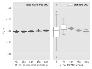
Figure 2. Logistic regression: estimates of the normalising constant obtained from waste-free SMC ($N=2\times 10^{5}$) and standard SMC ($N=2\times 10^{5}/k$).

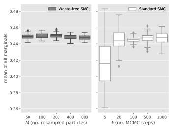
Figure 3. Same plot as Figure 2 for the estimate of the posterior expectation of the mean of all coordinates.

These figures deserve several comments. First, waste-free seems to perform best in the “long chain” regime, when $M\ll N$. Second, within this regime, the performance seems robust to the choice of $M$; notice how the same level of performance is obtained whether $M=50$ or $M=400$ (similar performance is also obtained for $M<50$, results not shown. We focused on $M\geq 50$ for reasons related to parallel hardware as discussed in Section 4.1.) Third, in contrast, it seems difficult to choose $k$ to obtain optimal performance; notice in particular that Figure 3 suggests to take $k=100$, but, for this value of $k$, the estimate of the log-normalising constant seems biased, see Figure 2. (Interestingly, we observed such an upward bias for all values of $k$ when we ran standard SMC for a smaller value of $N$, $N=10^{5}$; hence standard SMC seems also slightly less robust to the choice of $N$; results not shown.) Fourth, and perhaps most importantly, we are able to obtain better performance from waste-free SMC for a given CPU budget.

We now evaluate the performance of the variance estimates discussed in Section 4.3. Figure 4 shows box-plots of these estimates obtained from 100 runs of waste-free SMC, for $N=2\times 10^{5}$ and $M=50$: the $M-$chain estimate advocated in Section 4.3; the estimate of Olsson and Douc, (2019), with a lag of 3 (the biased, but more stable version of Lee and Whiteley, (2018), as explained in Section 4.3) and finally, the empirical variance over 10 independent runs. All these variance estimates are re-scaled by the same factor, such that the empirical variance over the 100 runs equals one. (Other values for the lag in the method of Olsson and Douc, (2019) did not seem to give better results.)

Clearly, the $M-$chain estimator is more satisfactory, as it performs better (especially for the normalising constant, left plot) than the empirical variance, although being computed from a single run. On the other hand, the approach of Lee and Whiteley, (2018) performs poorly. To be fair, this approach works more reasonably if we increase significantly $M$ (results not shown), but since taking $M$ too large decreases the performance of the algorithm, it seems fair to state that this approach is not useful for waste-free SMC, at least in this example.

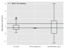
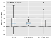
Figure 4. Logistic regression: box-plots of variance estimates over 100 runs obtained with waste-free SMC. Left: variance of the log-normalising constant estimate. Right: variance of the mean of all coefficients estimate. The variance estimates are re-scaled so that the empirical variance over the 100 runs equals one; see text for more details.

5.2. Latin squares

Our second example concerns the enumeration of Latin squares of size $d$; that is, $d\times d$ matrices with entries in $\{0,\ldots,d-1\}$, and such that each integer in that range appears exactly once in each row and in each column; see Table 1 for an example. The number $l(d)$ of Latin squares of size $d$ increases very quickly with $d$, and is larger than $10^{43}$ for $d=11$, the largest value for which it is known; see sequence A002860 of the OEIS database (OEIS Foundation Inc.,, 2020).

1	5	0	3	7	8	9	6	2	4
0	4	5	8	6	9	1	7	3	2
2	8	7	0	9	4	5	3	1	6
3	7	4	1	5	2	8	0	6	9
6	0	9	5	1	3	2	8	4	7
8	2	1	9	4	0	6	5	7	3
9	6	3	2	0	5	7	4	8	1
5	1	6	4	3	7	0	2	9	8
4	9	2	7	8	6	3	1	5	0
7	3	8	6	2	1	4	9	0	5

Table 1. A Latin square of size $10$

Let $\mathcal{X}$ be the set of permutation squares of size $d$, that is, $d\times d$ matrices such that each row is a permutation of $\{0,\ldots,d-1\}$, and let $p(d)$ its cardinal, $p(d)=(d!)^{d}$. We consider the following sequence of tempered distributions: $\pi_{t}(\mathrm{d}x)=\nu(\mathrm{d}x)\exp\{-\lambda_{t}V(x)\}/L_{t}$, where $\nu(\mathrm{d}x)$ stands for the uniform distribution over $\mathcal{X}$, and $V$ is a certain score function such that $V(x)=0$ if $x$ is a Latin square, $V(x)\geq 1$ otherwise. Specifically, denoting the entries of matrix $x$ by $x[i,j]$, we take

$$V(x)=\sum_{j=1}^{d}\left\{\sum_{l=1}^{d}\left(\sum_{i=1}^{d}\mathbb{1}(x[i,j]=l)\right)^{2}-d\right\}.$$

The quantity $L_{t}\times p(d)$ will be at distance $\varepsilon$ of $l(d)$, the number of Latin squares, as soon as $\lambda_{t}\geq\log(p(d)/\varepsilon)$. Thus, we select adaptively the successive exponents $\lambda_{t}$ (as in the previous example), and stop the algorithm at the first iteration $t$ such that this condition is fulfilled, for $\varepsilon=10^{-16}$.

We set the Markov kernel $M_{t}$ to be a $k$-fold Metropolis kernel based on the following proposal distribution: given $x$, select randomly a row $i$, two columns $j$, $j^{\prime}$, and swap components $x[i,j]$ and $x[i,j^{\prime}]$.

Figure 5 compares the performance of standard SMC and waste-free SMC for evaluating the log of the normalising constant $L_{T}$, that is (up to a small error as explained above), the log of the number of Latin squares $l(d)$; we take $d=11$ since this is the largest value of $d$ for which $l(d)$ is known exactly.

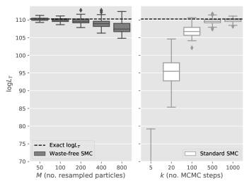
Figure 5. Latin squares: box-plots of estimates of $\log L_{T}$ (log of number of Latin squares) obtained from 100 independent runs of the following algorithms: waste-free SMC ($N=2\times 10^{5}$, different values of $M$, the number of resampled particles), and standard SMC ($N=2\times 10^{5}/k$, different values for $k$, the number of MCMC steps).

As in the previous example, the compared algorithms are given (roughly) the same CPU budget: $N=2\times 10^{5}/k$ for standard SMC, while $N=2\times 10^{5}$ for waste-free (and $k=1$, as already discussed). We make the same observations as in the previous example: best performance is obtained from waste-free SMC in the long chain regime ($M\ll N$), and, within this regime, performance does not seem to depend strongly on $M$.

One distinctive feature of this example is that the mixing of the Metropolis kernel used to move the particles significantly decreases over time; see Figure 6, which plots the acceptance rate of that kernel at each iteration $t$ of a waste-free SMC run.

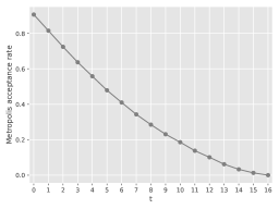
Figure 6. Latin squares: acceptance rate of the Metropolis kernel described in the text at each iteration $t$ of a run of waste-free SMC.

It is interesting to note that waste-free SMC seems to work well despite this. Unfortunately, it does seem to affect the performance of our $M-$chain variance estimate. The left panel of Figure 7 makes the same comparison as Figure 4 in our first example. This time, however, the $M-$chain estimator seems to be biased downward, by a factor of two. This bias seems to originate from the terms of for the last values of $t$; these terms are both larger, and more difficult to estimate if $P$ is not large enough.

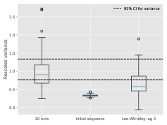
Figure 7. Latin squares: same plot as Figure 4, for the estimate of log-normalising constant $\log L_{T}$. Left: non-adaptive version ($M=50$, $N=2\times 10^{5}$); Right: adaptive version ($M=50$, $N_{0}=5$). See text for more details.

These results showcase the interest of adapting $P$ across time, as discussed in Section 4.4. We re-run waste-free SMC for the same problem, with $M=50$, and $\kappa=5$; that is, at each iteration $t$, $P_{t}$ is adjusted to be close to $\kappa$ times the auto-correlation time, for function $\bar{G}_{t}$. The right side of Figure 7 repeats the comparison of the variance estimates, but for the adaptive $P$ algorithm. This time, our $M-$chain estimate seems to perform satisfactorily.

In addition, Figure 8 compares the CPU vs error trade-off for both variants of waste-free SMC. In both cases, we set $M=50$; “CPU time” on the x-axis is measured by the number of calls to the score function, re-scaled so that the smallest observed value is 1. (Both axis use a $\log 2$-scale.) Each dot corresponds to an average over 100 runs. For the vanilla version, we set $N=6250$, $2.5\times 10^{4}$, $10^{5}$, $4\times 10^{5}$ and $8\times 10^{5}$. For the adaptive version, we set $\kappa=2$, 5 and 10. The dotted lines have slope $-1$. For high CPU time both algorithms show the same level of performance. If $N$ is set to too low a value for vanilla waste-free (e.g. $N=6250$), then one obtains a very large MSE, because $P=N/M=125$ is too small relative to the auto-correlation time of the kernels $M_{t}$ for large $t$. Note that for the adaptive version, it does not make sense to take $\kappa\ll 2$, as one cannot properly estimate the auto-correlation time of a chain without running it for a length commensurate with its auto-correlation time. In a sense, the adaptive version of waste-free prevents us from setting $P$ to too low a value, where performance becomes sub-optimal.

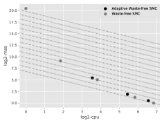
Figure 8. Latin squares: MSE (mean square error) vs CPU time (number of calls to score function), averaged over 100 independent runs of vanilla waste-free (grey dots, $N=6250$, $2.5\times 10^{4}$, $10^{5}$, $4\times 10^{5}$, $8\times 10^{5}$), and adaptive waste-free (black dots, $\kappa=2$, $5$, $10$). Both axes use a $\log 2-$scale; parallel dotted lines have slope $-1$.

By and large, in any problem when there is some evidence that the mixing of kernels $M_{t}$ may decrease significantly over time, we recommend to use the adaptive $P$ strategy. It is a bit less practical to use, as it gives less control to the user on the running time of the algorithm; but on the other hand it seems to provide more reliable variance estimates in this kind of scenario.

5.3. Orthant probabilities

Finally, we consider the problem of evaluating Gaussian orthant probabilities, i.e. $p(a,\Sigma):=\mathbb{P}(Z\geq a)$, where $a\in\mathbb{R}^{d}$, $Z\sim\mathcal{N}_{d}(0,\Sigma)$, and $\Sigma$ is a covariance matrix of size $d\times d$.

Ridgway, (2016) developed the following SMC approach for evaluating such probabilities. Let $\Gamma$ be the lower triangle in the Cholesky decomposition of $\Sigma$: $\Sigma=\Gamma\Gamma^{T}$; $\Gamma=(\gamma_{ij})$ and $\gamma_{ii}>0$ for all $i$. The orthant probability $p(a,\Sigma)$ may be rewritten as the joint probability that $X_{t}\geq f_{t}(X_{1:t-1})$ for $t=1,\ldots,d$, where $f_{t}(x_{1:t-1})=(a_{t}-\sum_{s<t}\gamma_{st}x_{s})/\gamma_{tt}$, and the $X_{t}$’s are IID $\mathcal{N}(0,1)$ variables. (At time $1$, $f_{1}(x_{1:0})$ is simply $a_{1}$, i.e. the constraint is $X_{1}\geq a_{1}$.)

The SMC algorithm of Ridgway, (2016) applies the following operations to particles $X_{1:t}^{n}$, from time $1$ to time $T=d$. (We change notations slightly and start at time 1, for the sake of readability.) (a) At time $t$, particles $X_{1:t-1}^{n}$ are extended by sampling an extra component, $X_{t}^{n}$, from a univariate truncated Gaussian distribution (the distribution of $X_{t}\sim N(0,1)$ conditional on $X_{t}\geq f_{t}(x_{0:t-1})$); (b) particles $X_{1:t}^{n}$ are then reweighted according to function $\Phi(-f_{t}(X_{1:t-1}^{n}))$, where $\Phi$ is the $\mathcal{N}(0,1)$ cumulative distribution function; and (c) when the ESS (effective sample size) of the weights gets too low, the particles are moved through $k$ iterations of a certain MCMC kernel that leaves invariant $\pi_{t}$, the distribution that corresponds to $X_{1:t}\sim N_{t}(0,I_{t})$ constrained to $X_{s}\geq f_{s}(X_{1:s-1})$ for $s=1,\ldots,t$. Based on numerical experiments, Ridgway, (2016) recommended to use for the MCMC kernel at time $t$ a Gibbs sampler that leaves $\pi_{t}$ invariant. (the update of each variable amounts to sampling from a univariate truncated normal distribution.)

This SMC algorithm does not fit in the framework of Algorithm 1; in particular the dimension of the state-space $\mathcal{X}=\mathbb{R}^{t}$ increases over time. However, we can easily generalise waste-free SMC to this setting: whenever an MCMC rejuvenation step is applied, resample $M\ll N$ particles, apply $P-1$ steps of the chosen MCMC kernels to these $M$ resampled particles, and gather the $N=MP$ so obtained values to form the new particle sample.

To make the problem challenging, we take $d=150$, $a=(1.5,1.5,\ldots)$, and $\Sigma$ a random correlation matrix with eigenvalues uniformly distributed in the simplex $\left\{x_{1}+\cdots+x_{d}=150,x_{i}\geq 0\right\}$, which we simulated using the algorithm of Davies and Higham, (2000). As in Ridgway, (2016), before the computation we re-order the variables according to the heuristic of Gibson et al., (1994).

Figures 9 and 10 do the same comparison of standard SMC and waste-free SMC as in the two previous examples: $N=2\times 10^{5}$ for waste-free, $N=2\times 10^{5}/k$ for standard SMC, and $M$ (resp. $k$) varies over a range of values. Figure 9 plots box-plots of estimates of $\log L_{T}$ (the log of the orthant probability), while Figure 10 does the same for $\mathbb{Q}_{T}(\varphi)$, with $\varphi(x_{0:T})=(\sum_{t=0}^{T}x_{t})/T$; i.e. the expectation of $\varphi$ with respect to the corresponding truncated Gaussian distribution.

We observe again that waste-free SMC outperforms standard SMC, at least whenever $M\ll N$. In addition, the greater robustness of waste-free is quite striking in this example.

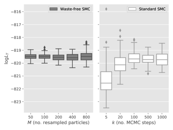
Figure 9. Orthants: estimates of the log normalizing constant obtained from waste-free SMC ($N=2\times 10^{5}$) and standard SMC ($N=2\times 10^{5}/k$).

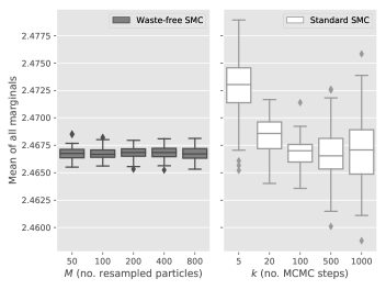
Figure 10. Orthants: Same plot as Figure 9 for $\mathbb{Q}_{T}(\varphi)$, the expectation of function $\varphi(x_{0:T})=(\sum_{t=0}^{T}x_{t})/T$ with respect to truncated Gaussian distribution $\mathcal{N}_{>0}(a,\Sigma)$.

Finally, Figure 11 compares $M-$chain estimators of the variance of the orthant probability estimate based on two single-chain estimators: the initial sequence estimator we recommended by default in Section 4.3, and we used in the two previous examples; and a spectral estimator based on the Tukey-Hanning window (see e.g. Flegal and Jones,, 2010). In this example, the kernels $M_{t}$ are Gibbs kernels, and are therefore not reversible. This seems to explain the poor performance of the former.

(As in previous plots, Figures 4 and 7, we include for comparison the variance estimator obtained by taking an empirical variance over 10 runs; however we do not include, for the sake of readability, the estimator based on Lee and Whiteley, (2018), but note simply it performs poorly in this case too.)

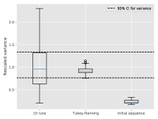
Figure 11. Orthants: box-plots of variance estimates over 100 runs for the estimate of the log orthant probability. The variance estimates are re-scaled so that the empirical variance over the 100 runs equals one; see text for more details.

6. Concluding remarks

6.1. Connection with nested sampling

In our definition of waste-free SMC, we took $N=MP$, with $P\geq 2$; thus $M$ divides $N$. We may generalise the algorithm to any pair $(M,N)$, $M<N$: at time $t$, resample $M$ particles, generate $M$ chains of length $k:=\lfloor N/M\rfloor$ (using kernel $M_{t}$, and the resampled particles as the starting points); then select (without replacement) $N-Mk$ chains and extend them to have length $k+1$. The total number of particles is then $N$.

One interesting special case is $M=N-1$. In that case, $N-1$ particles are resampled (thus at least one particle is discarded), and, among these $N-1$ resampled particles, only one particle is moved through kernel $M_{t}$. In addition, if the target distributions $\pi_{t}$ are of the form $\pi_{t}(\mathrm{d}x)\propto\nu(\mathrm{d}x)\mathbb{1}\{L(x)\geq l_{t}\}$, where $\nu$ is a prior distribution, and $L$ a likelihood function, then one recovers essentially the nested sampling algorithm of Skilling, (2006).

This raises the question whether the regime $M=N-1$ is useful, either for such a sequence of distributions, or more generally. For the former, the numerical experiments of Salomone et al., (2018) seem to indicate than standard SMC, when applied to this type of sequence, may perform as well as nested sampling. This suggests waste-free SMC should also perform at least as well as nested sampling, although we leave that point for further investigation. For the latter, we note that taking $M=N-1$ is not very convenient, as this means we move only one particle at each iteration, although each iteration costs $\mathcal{O}(N)$. (In nested sampling, the cost of a single iteration may be reduced to $\mathcal{O}(1)$ by using the fact that weights are either 0 or 1.)

6.2. Further work

Our convergence results assume that the kernels $M_{t}$ are uniformly ergodic. However, many practical MCMC kernels are not uniformly ergodic, hence it seems worthwhile to extend these results to, say, geometrically ergodic kernels. Another result we would like to establish is that waste-free SMC dominates standard SMC in terms of asymptotic variance, at least under certain conditions on the mixing of the kernels $M_{t}$.

In terms of applications, we wish to explore how waste-free may be implemented in various SMC schemes, in particular in the SMC² algorithm of Chopin et al., (2013). This algorithm is an SMC sampler with expensive Markov kernels (as a single step amounts to propagate a large number of particles in a “local” particle filter), hence the benefits brought by waste-free SMC may be particularly valuable in this type of scenario.

The original implementation of the numerical examples may be found at https://github.com/hai-dang-dau/waste-free-smc. Waste-free SMC is also now implemented in the particles library, see https://github.com/nchopin/particles.

Appendix A Proofs

A.1. Proof of Proposition 2

We may rewrite (6) as:

$$\prod_{s=0}^{t}\left\{\frac{1}{M}\sum_{m=1}^{M}\left(\frac{1}{P}\sum_{p=1}^{P}G_{s}(z_{s}^{m}[p])\right)\right\}$$

where $z_{s}^{m}[p]$ stands for variable $\tilde{X}_{s}^{m,p}$ which is defined inside Algorithm 2.

We recognise the normalising constant estimate of a standard SMC sampler, Algorithm 1, when applied to the waste-free Feynman-Kac model defined in Proposition 1. The expectation of this quantity is therefore the normalising constant $L_{t}^{\mathrm{wf}}=L_{t}$ (Proposition 1), since such estimates are unbiased (Del Moral,, 1996).

A.2. Proof of Proposition 4

We start by establishing two technical lemmas regarding a uniformly ergodic Markov chain $(X_{p})_{p\geq 0}$, $(X_{p})$ for short, on probability space $(\mathcal{X},\mathbb{X})$; i.e. $\left\lVert K^{k}(x,\mathrm{d}x^{\prime})-\pi(\mathrm{d}x^{\prime})\right\rVert_{\operatorname{TV}}\leq C\rho^{k}$ for certain constants $C>0$ and $\rho<1$ and a certain probability distribution $\pi$, where $K^{k}(x,\mathrm{d}x)$ stands for the $k-$fold Markov kernel that defines the distribution of $X_{p+k}$ given $X_{p}$. Then $\pi(\mathrm{d}x)$ is its stationary distribution.

Lemma 1.

Assume that $(X_{p})$ is stationary, i.e. $X_{0}\sim\pi(\mathrm{d}x)$, and therefore $X_{p}\sim\pi(\mathrm{d}x)$ for all $p\geq 0$. Then there exists a constant $C_{1}>0$ such that:

$$\mathrm{Var}\left(\varphi(X_{0})\right)+2\sum_{k=1}^{\infty}\left|\mathrm{Cov}\left(\varphi(X_{0}),\varphi(X_{k})\right)\right|\leq C_{1}\left\lVert\varphi\right\rVert_{\infty}^{2}$$

for any measurable bounded function $\varphi:\mathcal{X}\rightarrow\mathbb{R}$.

Proof.

One has

$$\left|\mathrm{Cov}\left(\varphi(X_{0}),\varphi(X_{k})\right)\right| =\left|\mathbb{E}[\varphi(X_{0})\varphi(X_{k})]-\mathbb{E}[\varphi X_{0}]\mathbb{E}[\varphi X_{k}]\right|$$

$$=\left|\int\left\{\int\varphi(x_{k})K^{k}(x_{0},\mathrm{d}x_{k})-\int\varphi(x_{k})\pi(\mathrm{d}x_{k})\right\}\varphi(x_{0})\pi(\mathrm{d}x_{0})\right|$$

$$\leq 2\rho^{k}C\left\lVert\varphi\right\rVert_{\infty}^{2}$$

from which the result follows. ∎

In the second lemma, the distribution of the initial state $X_{0}$ is arbitrary, and therefore the chain is not necessarily stationary.

Lemma 2.

There exists a constant $C_{2}>0$ (which does not depend on the initial distribution of the chain, i.e. the distribution of $X_{0}$), such that

$$\mathrm{Var}\left(\frac{1}{P}\sum_{p=1}^{P}\varphi(X_{p})\right)\leq C_{2}\frac{\left\lVert\varphi\right\rVert_{\infty}^{2}}{P}$$

for any $P\geq 1$ and any bounded measurable function $\varphi:\mathcal{X}\rightarrow\mathbb{R}$.

Proof.

The proof relies on a standard coupling argument, see e.g. Chapter 19 of Douc et al., (2018). We introduce an arbitrary integer $R$, $1\leq R\leq P$, and a Markov chain $(X_{p}^{\star})$ constructed as follows: (a) $X_{0}^{\star}\sim\pi(\mathrm{d}x)$, the stationary distribution of $(X_{p})$; (b) variables $X_{R}$, $X_{R}^{\star}$ are maximally coupled, which implies that:

(18) $$\mathbb{P}(X_{R}\neq X_{R}^{\star})=\left\lVert\int\mu(\mathrm{d}x_{0})K(x_{0},\mathrm{d}x_{p})-\pi(\mathrm{d}x_{p})\right\rVert_{\operatorname{TV}}\leq C\rho^{R}$$

where $\mu(\mathrm{d}x_{0})$ denotes the probability distribution of $X_{0}$, and the inequality stems from the uniform ergodicity of the chain; (c) if $X_{R}=X_{R}^{\star}$, the two chains remain equal until time $P$, otherwise they are independent; (d) the distribution of $X_{1}^{\star},\ldots,X_{R-1}^{\star}$ given $X_{0}^{\star}$, $X_{R}^{\star}$ is the conditional distribution of these states induced by $K(x,\mathrm{d}x^{\prime})$, the Markov kernel of $(X_{p})$. For more details on maximal coupling of two probability distributions, see e.g. Chap. 19 of Douc et al., (2018).

Using the inequality $\mathrm{Var}(X+Y+Z)\leq 3(\mathrm{Var}(X)+\mathrm{Var}(Y)+\mathrm{Var}(Z))$, we have:

$$\mathrm{Var}\left(\frac{1}{P}\sum_{p=1}^{P}\varphi(X_{p})\right) \leq 3\mathrm{Var}\left(\frac{1}{P}\sum_{p=1}^{P}\varphi(X_{p}^{\star})\right)+3\mathrm{Var}\left(\frac{1}{P}\sum_{p=1}^{R}\left\{\varphi(X_{p})-\varphi(X_{p}^{\star})\right\}\right)$$

$$+3\mathrm{Var}\left(\mathbb{1}\{X_{R}\neq X_{R}^{\star}\}\frac{1}{P}\sum_{p=R}^{P}\left\{\varphi(X_{p})-\varphi(X_{p}^{\star})\right\}\right)$$

$$\leq\frac{3C_{1}\left\lVert\varphi\right\rVert_{\infty}^{2}}{P}+\frac{12R^{2}\left\lVert\varphi\right\rVert_{\infty}^{2}}{P}+C\rho^{R}\left\lVert\varphi\right\rVert_{\infty}^{2}$$

where we have applied Lemma 1 to the first term, and (18) to the third term. We conclude by taking $R=\lceil\sqrt{P}\rceil$.

∎

We now prove Proposition 4 by induction. Clearly, (11) holds at time $0$. The implication (11) $\Rightarrow$ (12) at time $t$ follows the same lines as for a standard SMC sampler, see e.g. Section 11.2.2 in Chopin and Papaspiliopoulos, (2020). Now assume that (12) holds at time $t-1\geq 0$, and let $\bar{\varphi}=\varphi-\mathbb{Q}_{t-1}(\varphi)$, $\mathcal{F}_{t-1}=\sigma(X_{t-1}^{1:N})$ (the $\sigma$-field generated by variables $X_{t-1}^{n}$, $n=1,\ldots,N$). Then

$$\mathbb{E}\left[\left.{\left(\frac{1}{N}\sum_{n=1}^{N}\varphi(X_{t}^{n})-\mathbb{Q}_{t-1}(\varphi)\right)^{2}}\right|{\mathcal{F}_{t-1}}\right]$$

$$=\mathbb{E}\left[\left.{\left(\frac{1}{M}\sum_{m=1}^{M}\frac{1}{P}\sum_{p=1}^{P}\bar{\varphi}(\tilde{X}_{t}^{m,p})\right)^{2}}\right|{\mathcal{F}_{t-1}}\right]$$

$$=\left(\mathbb{E}\left[\left.{\frac{1}{P}\sum_{p=1}^{P}\bar{\varphi}(\tilde{X}_{t}^{1,p})}\right|{\mathcal{F}_{t-1}}\right]\right)^{2}+\frac{1}{M}\mathrm{Var}\left(\left.{\frac{1}{P}\sum_{p=1}^{P}\bar{\varphi}(X_{t}^{1,p})}\right|{\mathcal{F}_{t-1}}\right)$$

since the blocks of variables $X_{t}^{m,1:P}$ are IID (independent and identically distributed) conditional on $\mathcal{F}_{t-1}$.

The expectation of the first term may be bounded by $c^{\prime}_{t-1}\left\lVert\varphi\right\rVert_{\infty}^{2}/N$ by applying (12) to function $P^{-1}\sum_{p=0}^{P-1}M_{t}^{p}\varphi$. The second term may be bounded by $C_{2}\left\lVert\varphi\right\rVert_{\infty}^{2}/N$ using Lemma 2.

A.3. Proof of Theorem 1

We start by proving a few basic lemmas. The first one concerns product measures. We use symbol $\bigotimes$ throughout to represent the product of two probability measures.

Lemma 3 (Total variation distance for product measure).

Let $\mu_{1:N}$ and $\nu_{1:N}$ be $2N$ probability measures on $(\mathcal{X},\mathbb{X})$. Then the following inequality holds:

$$\left\lVert\bigotimes_{n=1}^{N}\mu_{n}-\bigotimes_{n=1}^{N}\nu_{n}\right\rVert_{\operatorname{TV}}\leq\sum_{n=1}^{N}\left\lVert\mu_{n}-\nu_{n}\right\rVert_{\operatorname{TV}}.$$

Proof.

Take $N=2$. Then

$$\left\lVert\mu_{1}\otimes\mu_{2}-\nu_{1}\otimes\nu_{2}\right\rVert_{\operatorname{TV}}\leq\left\lVert\mu_{1}\otimes\mu_{2}-\mu_{1}\otimes\nu_{2}\right\rVert_{\operatorname{TV}}+\left\lVert\mu_{1}\otimes\nu_{2}-\nu_{1}\otimes\nu_{2}\right\rVert_{\operatorname{TV}}$$

and we may bound the first term as follows:

$$\left\lVert\mu_{1}\otimes\mu_{2}-\mu_{1}\otimes\nu_{2}\right\rVert_{\operatorname{TV}}$$

$$=\sup_{f:\mathcal{X}^{2}\to[0,1]}\left|\int\left(\int f(x,y)\mu_{1}(\mathrm{d}x)\right)\mu_{2}(\mathrm{d}y)-\int\left(\int f(x,y)\mu_{1}(\mathrm{d}x)\right)\nu_{2}(\mathrm{d}y)\right|$$

$$\leq\sup_{g:\mathcal{X}\to[0,1]}\left|\int g(y)\mu_{2}(\mathrm{d}y)-\int g(y)\nu_{2}(\mathrm{d}y)\right|=\left\lVert\mu_{2}-\nu_{2}\right\rVert_{\operatorname{TV}}.$$

The result follows by bounding the second term similarly. For $N\geq 3$, proceed recursively. ∎

The two next lemmas concern the behaviour of $M\geq 1$ independent, stationary, Markov chains, $(Y_{p}^{m})_{p\geq 0}$ on $(\mathcal{X},\mathbb{X})$, $m=1,\ldots,M$ with uniformly ergodic Markov kernel $K$, and invariant distribution $\pi$: $\left\lVert\delta_{x}K^{p}-\pi\right\rVert_{\operatorname{TV}}\leq C\rho^{k}$ for constants $C\geq 0$ and $\rho\in[0,1)$.

Lemma 4.

The product kernel

$$K^{\otimes M}(x_{1:M},\mathrm{d}x^{\prime}_{1:M})=\prod_{m=1}^{M}K(x_{m},\mathrm{d}x^{\prime}_{m})$$

is uniformly ergodic, with stationary distribution $\pi^{\otimes M}$.

Proof.

This is a direct consequence of Lemma 3:

$$\left\lVert\delta_{x_{1:M}}\left(K^{\otimes M}\right)^{p}-\pi^{\otimes M}\right\rVert_{\operatorname{TV}} \leq\sum_{m=1}^{M}\left\lVert\delta_{x_{m}}K^{p}-\pi\right\rVert_{\operatorname{TV}}$$

$$\leq CM\rho^{p}.$$

∎

Lemma 5.

For $\varphi:\mathcal{X}\rightarrow\mathbb{R}$ measurable and bounded, one has:

$$\sqrt{MP}\left(\frac{\sum_{m=1}^{M}\sum_{p=1}^{P}\varphi(Y_{p}^{m})}{MP}-\pi(\varphi)\right)\Rightarrow\mathcal{N}\left(0,v_{\infty}(K,\varphi)\right)$$

as $P\rightarrow+\infty$, whether $M\geq 1$ is fixed, or $M$ grows with $P$; i.e. $M=M(P)\rightarrow+\infty$ as $P\rightarrow+\infty$.

Proof.

For $M=1$, this is simply the classical central limit theorem for uniformly ergodic Markov chains, see e.g. Theorem 23 in Roberts and Rosenthal, (2004) and references therein. For $M\geq 2$ fixed, we may apply the same theorem to the Markov chain $(Y_{p}^{1:M})_{p}$ in $(\mathcal{X}^{M},\mathbb{X}^{M})$, which is also uniformly ergodic (Lemma 4) and to test function $\varphi_{M}(y^{1:M})=M^{-1}\sum_{m=1}^{M}\varphi(y^{m})$.

Assume now $M=M(P)$ grows with $P$. Let $\bar{\varphi}=\varphi-\pi(\varphi)$ and let $S_{P}$ denote a variable with the same distribution as $S_{P}^{m}:=P^{-1/2}\sum_{p=1}^{P}\bar{\varphi}(Y_{p}^{m})$ for $m=1,\ldots,M$. (These $M$ variables are IID.) By the formula (19) of Roberts and Rosenthal, (2004), we have $\mathbb{E}[S_{P}^{2}]\rightarrow v_{\infty}(K,\varphi)$. Therefore, fixing $u\in\mathbb{R}$, we wish to prove that $\Delta_{P}\rightarrow 0$, where

$$\Delta_{P}:=\left|\left(\mathbb{E}e^{iuS_{P}/\sqrt{M}}\right)^{M}-\left(1-\frac{u^{2}}{2M}\mathbb{E}(S_{P}^{2})\right)^{M}\right|.$$

Let $M_{0}\geq 1$ be fixed such that $u^{2}\mathbb{E}[S_{P}^{2}]/2M_{0}<1$ for all $P>M_{0}$. Since $\left|a^{M}-b^{M}\right|\leq M\left|a-b\right|$ for $\left|a\right|,\left|b\right|\leq 1$ and $\left|e^{ix}-1-ix+x^{2}/2\right|\leq\min(x^{2},|x^{3}|/6)$ for $x\in\mathbb{R}$, we have, for any $M\geq M_{0}$:

(19) $$\Delta_{P}\leq\mathbb{E}\min\left(u^{2}S_{P}^{2},\frac{\left|u^{3}S_{P}^{3}\right|}{6\sqrt{M}}\right)\leq\mathbb{E}f_{M_{0}}(S_{P})$$

where $f_{m}(x):=\min\left(u^{2}x^{2},\left|u^{3}x^{3}/6\sqrt{m}\right|\right)=f_{m}^{1}(x)+f_{m}^{2}(x)$, $f_{m}^{1}(x):=u^{2}x^{2}$ and $f_{m}^{2}(x):=\mathbb{1}_{\left|x\right|\leq 6\sqrt{m}/\left|u\right|}\left(\left|u^{3}x^{3}\right|/6\sqrt{m}-u^{2}x^{2}\right)$. Then, if $G$ is a Gaussian variable with variance $v_{\infty}(K,\varphi)$, we have $\mathbb{E}f^{1}_{M_{0}}(S_{P})\to\mathbb{E}f^{1}_{M_{0}}(G)$ as $P\rightarrow+\infty$. Moreover, $\mathbb{E}f^{2}_{M_{0}}(S_{P})\to\mathbb{E}f^{2}_{M_{0}}(G)$ by Theorem 23 of Roberts and Rosenthal, (2004) and the fact that $f^{2}_{M_{0}}$ is a bounded function and is only discontinuous on a set of measure zero with respect to a Gaussian distribution. Thus (19) implies that $\limsup_{P\to\infty}\Delta_{P}\leq\mathbb{E}f_{M_{0}}(G)$. But $\mathbb{E}f_{M_{0}}(G)\to 0$ as $M_{0}\to\infty$ by the dominated convergence theorem, hence $\Delta_{P}\to 0$ and the lemma is proved. ∎

We now prove Theorem 1. We proceed by induction: (13) at time 0 is simply the standard central limit theorem for IID variables. The implication (13) $\Rightarrow$ (14) at time $t$ may be established exactly as in other proofs for central limit theorems for SMC algorithms; see e.g. Section 11.3 of Chopin and Papaspiliopoulos, (2020).

We now assume that (14) holds at time $t-1\geq 0$, and we wish to show that (13) holds at time $t$, or, equivalently, that:

(20) $$\frac{1}{\sqrt{P}}\sum_{p=1}^{P}\varphi_{M}(Z_{p})\Rightarrow\mathcal{N}\left(0,v_{\infty}(M_{t},\varphi)\right)$$

where (dropping the dependence on $t$ as it is fixed) $Z_{p}:=(\tilde{X}_{t}^{1,p},\ldots,\tilde{X}_{t}^{M,p})$ is a Markov chain on $\mathcal{X}^{M}$, which is uniformly ergodic (Lemma 4), and $\varphi_{M}(z)=M^{-1/2}\sum_{m=1}^{M}\bar{\varphi}(z[m])$.

We apply the coupling construction we used in the proof of Lemma 2 to this Markov chain: we introduce a stationary Markov chain, $(Z_{p}^{\star})$, with the same Markov kernel as $(Z_{p})$, i.e. $M_{t}^{\otimes M}$, which is coupled to $(Z_{p})$ at time $R$, $1\leq R\leq P$, with maximum coupling probability:

(21) $$\mathbb{P}(Z_{R}\neq Z_{R}^{\star})=\left\lVert\mathcal{L}(Z_{1})(M_{t}^{\otimes M})^{R}-\pi_{t-1}^{\otimes M}\right\rVert_{\operatorname{TV}}\leq MC\rho^{R}$$

If the two chains are successfully coupled at time $R$, they remain equal at times $R+1,\ldots,P$.

We decompose the left-hand side of (20) as:

(22) $$\frac{1}{\sqrt{P}}\sum_{p=1}^{P}\varphi_{M}(Z_{p})=\frac{1}{\sqrt{P}}\sum_{p=1}^{P}\varphi_{M}(Z_{p}^{\star})+\frac{1}{\sqrt{P}}\sum_{p=1}^{R}\varphi_{M}(Z_{p})\\ -\frac{1}{\sqrt{P}}\sum_{p=1}^{R}\varphi_{M}(Z_{p}^{\star})+\frac{1}{\sqrt{P}}\mathbb{1}\{Z_{R}\neq Z_{R}^{\star}\}\sum_{p=R+1}^{P}\left(\varphi_{M}(Z_{p})-\varphi_{M}(Z_{p}^{\star})\right).$$

The first terms converges to $\mathcal{N}\left(0,v_{\infty}(M_{t},\varphi)\right)$, see Lemma 5. What remains to prove is that the three other terms converge to zero in probability.

The fourth term is non-zero with probability (21), and tends to zero as soon as $R\rightarrow+\infty$; e.g. $R=\mathcal{O}(P^{\beta})$, $\beta\in(0,1)$. Using the inequality $\mathrm{Var}(Y_{1}+\ldots+Y_{R})\leq R\left(\mathrm{Var}(Y_{1})+\ldots+\mathrm{Var}(Y_{R})\right)$, we may bound the the $L^{2}$ norm of the third term as follows:

$$\mathrm{Var}\left(\frac{1}{\sqrt{P}}\sum_{p=1}^{R}\varphi_{M}(Z_{p}^{\star})\right)\leq\frac{R^{2}}{P}\mathrm{Var}_{\pi}(\bar{\varphi})\leq 2\frac{R^{2}}{P}\left\lVert\varphi\right\rVert_{\infty}^{2}$$

which tends to zero as soon as $R^{2}\ll P$, e.g. $R=\mathcal{O}(P^{\beta})$, $\beta\in(0,1/2)$.

The second term equals:

(23) $$R\sqrt{\frac{M}{P}}\left(\frac{1}{M}\sum_{m=1}^{M}\frac{1}{R}\sum_{p=1}^{R}\bar{\varphi}(\tilde{X}_{t}^{m,p})\right)$$

and, since the $M$ chains $\tilde{X}_{t}^{m,1:P}$ are independent, for $m=1,\ldots,M$, conditional on $\mathcal{F}_{t-1}=\sigma(X_{t-1}^{1:N})$, we have:

$$\mathbb{E}\left[\left.{\left(\frac{1}{M}\sum_{m=1}^{M}\frac{1}{R}\sum_{p=1}^{R}\bar{\varphi}(X_{t}^{m,p})\right)^{2}}\right|{\mathcal{F}_{t-1}}\right]$$

$$=\left(\mathbb{E}\left[\left.{\frac{1}{R}\sum_{p=1}^{R}\bar{\varphi}(\tilde{X}_{t}^{1,p})}\right|{\mathcal{F}_{t-1}}\right]\right)^{2}+\frac{1}{M}\mathrm{Var}\left(\left.{\frac{1}{R}\sum_{p=1}^{R}\varphi(\tilde{X}_{t}^{m,p})}\right|{\mathcal{F}_{t-1}}\right)$$

$$\leq\left\{\mathbb{Q}_{t-1}^{N}\left(\frac{1}{R}\sum_{p=1}^{R}M_{t}^{p-1}\bar{\varphi}\right)\right\}^{2}+\frac{2}{M}\left\lVert\varphi\right\rVert_{\infty}^{2}$$

where $\mathbb{Q}_{t-1}^{N}(\varphi)=\sum_{n=1}^{N}W_{t-1}^{n}\varphi(X_{t-1}^{n})$.

The expectation of the first term can be bounded by a constant times $\left\lVert\varphi\right\rVert_{\infty}^{2}/N$ by Proposition 4, thus the $\mathbb{L}^{2}$ norm of (23) is $\mathcal{O}(R/\sqrt{MP})$, which tends to zero as soon $R^{2}\ll MP$. Taking $R=\mathcal{O}(P^{\beta})$, $\beta\in(0,1/2)$ therefore ensures that all the terms in (22), minus the first, goes to zero.

A.4. Proof of Theorem 2

Before proving Theorem 2, we need to define some new notations to work comfortably with the convergence of conditional distributions. We start with a simple example.

Most Markov chains used in MCMC algorithms admit a central limit theorem regardless of its starting point, i.e., one has, for a Markov chain $(Y_{p})$ with invariant distribution $\pi$, and and a fixed point $y_{1}$,

$$\left.\sqrt{P}\left(\frac{1}{P}\sum_{p=1}^{P}\varphi(Y_{p})-\pi(\varphi)\right)\right|Y_{1}=y_{1}\Rightarrow\mathcal{N}(0,\sigma^{2})$$

for some $\sigma^{2}$, as $P\to\infty$. For uniformly ergodic Markov chains, stronger results hold. For example, for any deterministic sequence $(y_{p})_{p=1}^{\infty}$:

$$\left.\sqrt{P}\left(\frac{1}{P}\sum_{p=1}^{P}\varphi(Y_{p})-\pi(\varphi)\right)\right|Y_{1}=y_{P}\Rightarrow\mathcal{N}(0,\sigma^{2}).$$

If instead of having a single Markov chain, we have $M=M(P)$ chains $(Y_{p}^{m})$, $m=1,\ldots,M$, running in parallel, then, provided that the number of chains $M$ is negligible compared to their length $P$, it is possible to average the result of $M$ chains to get a better one. Specifically, it can be shown that for any deterministic sequence $(y_{P}^{m})$ indexed by $m$ and $p$,

(24) $$\left.\sqrt{MP}\left(\frac{1}{M}\sum_{m=1}^{M}\frac{1}{P}\sum_{p=1}^{P}\varphi(Y_{p}^{m})-\pi(\varphi)\right)\right|Y_{1}^{1:M}=y_{P}^{1:M}\Rightarrow\mathcal{N}(0,\sigma^{2})$$

as $P\to\infty$. It is natural to reformulate (24) using the following simplified notation:

(25) $$\left.\sqrt{MP}\left(\frac{1}{M}\sum_{m=1}^{M}\frac{1}{P}\sum_{p=1}^{P}\varphi(Y_{p}^{m})-\pi(\varphi)\right)\right|Y_{1}^{1:M}\Rightarrow\mathcal{N}(0,\sigma^{2})$$

while keeping in mind that $M=M(P)$ and in particular the $\sigma$-algebra generated by $Y_{1}^{1:M}$ does not stay the same when $P\to\infty$. While the interpretation (24) of the notation of (25) is intuitive, a more rigorous formalization will make manipulations easier. That is the point of the following definition and lemma, which are simple specific cases of more general results in Sweeting, (1989). The difference with Sweeting, (1989) is that we prefer, if possible, to work with probability conditioned on an event, which is simpler than probability conditioned on a filtration or a variable.

Definition 1 (Convergence of conditional distributions).

Let $(X_{n})_{n=1}^{\infty}$ be a sequence of random variables and let $(\mathcal{F}_{n})_{n=1}^{\infty}$ be a sequence of $\sigma$-algebras (which are not necessarily nested as in a filtration). We say that the sequence $X_{n}|\mathcal{F}_{n}$ of conditional distributions converge as $n\rightarrow\infty$ to distribution $\pi$,

$$X_{n}|\mathcal{F}_{n}\Rightarrow\pi,$$

if for any sequence $(B_{n})_{n=1}^{\infty}$ of events such that $B_{n}\in\mathcal{F}_{n}$ and $\mathbb{P}(B_{n})>0$, we have $X_{n}|B_{n}\Rightarrow\pi$.

Lemma 6.

Under the notations of definition 1, we have, for any continuous bounded function $\varphi:\mathcal{X}\rightarrow\mathbb{R}$,

$$\mathbb{E}\left[\left.{\varphi(X_{n})}\right|{\mathcal{F}_{n}}\right]\stackrel{{\scriptstyle a.s.}}{{\rightarrow}}\pi(\varphi).$$

Remark. This result is in fact used in Sweeting, (1989) as the definition of convergence in conditional probability. As said above, we prefer Definition 1 as we find it more convenient to work with probability conditioned on events than probability conditioned on sigma-algebras.

Proof.

For some $\epsilon>0$, define the events $B_{n}$ as

$$B_{n}:=\left\{\mathbb{E}\left[\left.{\varphi(X_{n})}\right|{\mathcal{F}_{n}}\right]-\pi(\varphi)\geq\epsilon\right\}.$$

If $\mathbb{P}(B_{n})>0$, one can write, since $B_{n}\in\mathcal{F}_{n}$:

(26) $$\mathbb{E}\left[\left.{\varphi(X_{n})}\right|{B_{n}}\right]=\mathbb{E}\left[\left.{\mathbb{E}\left[\left.{\varphi(X_{n})}\right|{\mathcal{F}_{n}}\right]}\right|{B_{n}}\right]\geq\pi(\varphi)+\epsilon.$$

If there exists an infinity of $n$ such that $\mathbb{P}(B_{n})>0$, we have by Definition 1 that $X_{n}|B_{n}\Rightarrow\pi$, which leads to a contradiction if we let $n\to\infty$ in both sides of (26). Thus, there exists some $n_{1}$ such that $\mathbb{P}(B_{n})=0,\forall n\geq n_{1}$. Similarly, one may show that there exists $n_{2}$ such that $\mathbb{P}(C_{n})=0$, $\forall n\geq n_{2}$, where

$$C_{n}=\left\{\mathbb{E}[\varphi(X_{n})|\mathcal{F}_{n}]-\pi(\varphi)<-\epsilon\right\}.$$

Now, note that the desired almost-sure convergence is equivalent to the fact that the random variable

$$R:=\limsup_{n\rightarrow\infty}\left|\mathbb{E}[\varphi(X_{n})|\mathcal{F}_{n}]-\pi(\varphi)\right|$$

equals $0$ almost surely. Indeed, for any $\epsilon>0$, the event $\left\{R\geq\epsilon\right\}$ is contained in $\left(\bigcup_{n=n_{1}}^{\infty}B_{n}\right)$ $\cup$ $\left(\bigcup_{n=n_{2}}^{\infty}C_{n}\right)$, which has probability zero. ∎

Lemma 7.

Let $(X_{n})_{n=1}^{\infty}$ and $(Y_{n})_{n=1}^{\infty}$ be two sequences of random variables such that $X_{n}\Rightarrow\mathbb{P}_{X}$ and $Y_{n}|X_{n}\Rightarrow\mathbb{P}_{Y}$ where the latter is understood in terms of Definition 1. Then $(X_{n},Y_{n})$ $\Rightarrow\mathbb{P}_{X}\otimes\mathbb{P}_{Y}$.

Proof.

Let $Y$ be a $\mathbb{P}_{Y}$-distributed random variable. We have that

$$\left|\mathbb{E}[e^{iuX_{n}+ivY_{n}}]-\mathbb{E}[e^{iuX_{n}}]\mathbb{E}[e^{ivY}]\right|=\left|\mathbb{E}\left[e^{iuX_{n}}\left(\mathbb{E}[e^{ivY_{n}}|X_{n}]-\mathbb{E}[e^{ivY}]\right)\right]\right|$$

tends to $0$ by dominated convergence theorem and the fact that $\mathbb{E}[e^{ivY_{n}}|X_{n}]-\mathbb{E}[e^{ivY}]$ converges almost surely to $0$ (Lemma 6). ∎

We are now able to prove Theorem 2.

Proof.

The idea of the proof is to show something very similar to (24). Indeed, we shall show the following conditional version of (20):

(27) $$\left.\frac{1}{\sqrt{P}}\sum_{p=1}^{P}\varphi_{M}(Z_{p})\right|\mathcal{F}_{t-1}\Rightarrow\mathcal{N}\left(0,v_{\infty}(M_{t},\varphi)\right)$$

which by Definition 1 means

(28) $$\left.\frac{1}{\sqrt{P}}\sum_{p=1}^{P}\varphi_{M}(Z_{p})\right|B_{t-1}\Rightarrow\left(0,v_{\infty}(M_{t},\varphi)\right)$$

for any sequence $B_{t-1}$ (implicitly indexed by $P$) of events such that $B_{t-1}^{P}\in\mathcal{F}_{t-1}^{P}$. The left hand side of (28) can be decomposed into four terms as in (22), where now $(Z_{p}^{\star})$ is a stationary Markov chain constructed via a maximal coupling of $\mathbb{Q}_{t-1}^{\otimes M}$ and the conditional (instead of the full) distribution of $Z_{R}$. The first, third and the fourth terms of (22) can be treated exactly as before. The second term tends to $0$ in probability when $R=N^{\epsilon}$ for small enough $\epsilon$, because $M=O(N^{\alpha})$ for $\alpha<1/2$. Thus (27) holds. Applying it for $\varphi=G_{t}$ and using the delta method give the convergence of $\sqrt{N}(\log\hat{\ell}_{t}-\log\ell_{t})|\mathcal{F}_{t-1}$ with asymptotic variance $v_{\infty}(M_{t},\bar{G}_{t})$. Furthermore, note that by Definition 1, the convergence of $X_{N}|\mathcal{F}_{N}$ implies the convergence of $X_{N}|\mathcal{F}^{\prime}_{N}$ if $\mathcal{F}^{\prime}_{n}\subset\mathcal{F}_{n}$ for all $n$. Hence

(29) $$\left.\sqrt{N}\left(\log\ell_{t}^{N}-\log\ell_{t}\right)\right|\sqrt{N}\left(\log L_{t-1}^{N}-\log L_{t-1}\right)\Rightarrow\mathcal{N}\left(0,v_{\infty}(M_{t},\bar{G}_{t})\right).$$

We can now proceed by induction. Suppose that the assertion is verified up to time $t-1$, that is,

(30) $$\sqrt{N}\left(\log L_{t-1}^{N}-\log L_{t-1}\right)\Rightarrow\mathcal{N}\left(0,\sum_{s=0}^{t-1}v_{\infty}(M_{s},\bar{G}_{s})\right).$$

Then, (29), (30) and Lemma 7 prove the assertion at time $t$. ∎

A.5. Proof of Proposition 5

We first calculate $\mathcal{V}^{\textrm{std,}k}_{t}(\varphi)$ by using e.g. formula (11.14) in Chopin and Papaspiliopoulos, (2020):

(31) $$\mathcal{V}^{\textrm{std,}k}_{t}(\varphi)=\sum_{s=0}^{t}\mathbb{Q}_{s-1}\left[\left\{\bar{G}_{s}R_{s+1:t}C_{t}\varphi\right\}^{2}\right]$$

where $\bar{G}_{t}=G_{t}/r$, $R_{t}(\varphi):=M_{t}\bar{G}_{t}\varphi$, $R_{s+1:t}:=R_{s+1}\circ\ldots\circ R_{t}$, and $C_{t}(\varphi):=\varphi-\mathbb{Q}_{t}(\varphi)$. Note that $M_{t}$, $\bar{G}_{t}$ and $C_{t}$ are all linear functionals. From the definition of $M_{t}$, we have

$$M_{t}(x_{t-1},B)=(1-\tilde{p}_{k})\mathbb{1}_{B}(x_{t-1})+\tilde{p}_{k}\pi_{t-1}(B),$$

with $\tilde{p}_{k}=1-(1-p)^{k}$, which leads to

$$\bar{G}_{s}R_{s+1:t}C_{t}\varphi=\bar{G}_{s}\left[\tilde{p}_{k}\mathbb{Q}_{s}^{\star}\bar{G}_{s+1}+(1-\tilde{p}_{k})\bar{G}_{s+1}\right]\ldots\left[\tilde{p}_{k}\mathbb{Q}_{t-1}^{\star}\bar{G}_{t}+(1-\tilde{p}_{k})\bar{G}_{t}\right]C_{t}\varphi.$$

It is easy to fully extend the above expression if one remarks that for any $l<t$, $\tilde{p}_{k}\mathbb{Q}_{l}^{\star}\bar{G}_{l+1:t}C_{t}\varphi=0$. Therefore only terms without any $\tilde{p}_{k}\mathbb{Q}_{l}^{\star}\bar{G}_{l+1}$ actually contribute to the result. Thus

$$\bar{G}_{s}R_{s+1:t}C_{t}\varphi=(1-\tilde{p}_{k})^{t-s}\bar{G}_{s:t}C_{t}\varphi.$$

We can now plug this into (31) and get

$$\mathcal{V}^{\textrm{std,}k}_{t}(\varphi) =\sum_{s=0}^{t}(1-\tilde{p}_{k})^{2(t-s)}\mathbb{Q}_{t-1}\left[\bar{G}_{s:t}^{2}(C_{t}\varphi)^{2}\right]$$

$$=\sum_{s=0}^{t}(1-\tilde{p}_{k})^{2(t-s)}\mathbb{Q}_{s-1}\left[\bar{G}_{s:t}\frac{1}{r^{t-s+1}}(C_{t}\varphi)^{2}\right]$$

$$=\sum_{s=0}^{t}\frac{1}{r}\left[\frac{(1-\tilde{p}_{k})^{2}}{r}\right]^{t-s}\mathbb{Q}_{t}\left[(C_{t}\varphi)^{2}\right]$$

$$=\frac{1}{r}\sum_{s=0}^{t}\left(\frac{(1-p)^{2k}}{r}\right)^{s}\mathrm{Var}_{\mathbb{Q}_{t}}(\varphi).$$

We thus see that the variance of the standard SMC sampler evolves proportionally to the sum of a geometric series and its stability depends on whether the base of the series is smaller than or greater than $1$. This proves the second point of the proposition. For the third point, note that

$$\mathcal{\tilde{V}}_{t}(\varphi) =\mathbb{Q}_{t-1}\left[(C_{t-1}\varphi)^{2}+2\sum_{s=1}^{\infty}(C_{t-1}\varphi)(K_{t}^{s}C_{t-1}\varphi)\right]$$

$$=\mathbb{Q}_{t-1}\left[(C_{t-1}\varphi)^{2}+2\sum_{s=1}^{\infty}(C_{t-1}\varphi)^{2}(1-p)^{s}\right]$$

$$=\left(\frac{2}{p}-1\right)\mathbb{Q}_{t-1}\left[(C_{t-1}\varphi)^{2}\right],$$

from which

$$\mathcal{V}^{\textrm{wf}}_{t}(\varphi) =\mathcal{\tilde{V}}_{t}(\bar{G}_{t}C_{t}\varphi)$$

$$=\left(\frac{2}{p}-1\right)\mathbb{Q}_{t-1}\left[(C_{t-1}\bar{G}_{t}C_{t}\varphi)^{2}\right]$$

$$=\left(\frac{2}{p}-1\right)\mathbb{Q}_{t-1}\left[(\bar{G}_{t}C_{t}\varphi)^{2}\right]$$

$$=\frac{1}{r}\left(\frac{2}{p}-1\right)\mathrm{Var}_{\mathbb{Q}_{t}}(\varphi).$$

Finally, to prove the last point of the proposition, we write

(32) $$\lim_{t\to\infty}\frac{\operatorname{IF}_{t}^{\textrm{wf}}}{k\operatorname{IF}_{t}^{\textrm{std,}k}}=\frac{r^{-1}(\frac{2}{p}-1)}{r^{-1}k\left(1-\frac{(1-p)^{2k}}{r}\right)^{-1}}\leq\left(\frac{2}{p}-1\right)\frac{1-(1-p)^{2k}}{k}$$

as the second to last expression is non-decreasing in $r$. Next, consider the function $f(p):=(1-p)^{2k}+2kp$ of which the derivative $f^{\prime}(p)=2k(1-(1-p)^{2k-1})$ is non-negative thanks to the fact that $k\geq 1$. We have $f(p)\geq f(0)=1$, which, when plugged into Equation (32), gives

$$\lim_{t\to\infty}\frac{\operatorname{IF}_{t}^{\textrm{wf}}}{k\operatorname{IF}_{t}^{\textrm{std,}k}}\leq\left(\frac{2}{p}-1\right)\frac{2kp}{k}\leq 4.$$

References

- Amzal et al., (2006) Amzal, B., Bois, F. Y., Parent, E., and Robert, C. P. (2006). Bayesian-optimal design via interacting particle systems. J. Amer. Statist. Assoc., 101(474):773–785.
- Berzuini et al., (1997) Berzuini, C., Best, N. G., Gilks, W. R., and Larizza, C. (1997). Dynamic conditional independence models and Markov chain Monte Carlo methods. J. Amer. Statist. Assoc., 92(440):1403–1412.
- Beskos et al., (2014) Beskos, A., Crisan, D., and Jasra, A. (2014). On the stability of sequential Monte Carlo methods in high dimensions. Ann. Appl. Probab., 24(4):1396–1445.
- Beskos et al., (2017) Beskos, A., Jasra, A., Law, K., Tempone, R., and Zhou, Y. (2017). Multilevel sequential Monte Carlo samplers. Stochastic Process. Appl., 127(5):1417–1440.
- Bornn et al., (2010) Bornn, L., Doucet, A., and Gottardo, R. (2010). An efficient computational approach for prior sensitivity analysis and cross-validation. Canad. J. Statist., 38(1):47–64.
- Buchholz et al., (2020) Buchholz, A., Chopin, N., and Jacob, P. E. (2020). Adaptive tuning of Hamiltonian Monte Carlo within sequential Monte Carlo. Bayesian Anal. Advance publication.
- Cérou et al., (2012) Cérou, F., Del Moral, P., Furon, T., and Guyader, A. (2012). Sequential Monte Carlo for rare event estimation. Stat. Comput., 22(3):795–808.
- Chan and Lai, (2013) Chan, H. P. and Lai, T. L. (2013). A general theory of particle filters in hidden Markov models and some applications. Ann. Statist., 41(6):2877–2904.
- Chopin, (2002) Chopin, N. (2002). A sequential particle filter method for static models. Biometrika, 89(3):539–551.
- Chopin et al., (2013) Chopin, N., Jacob, P. E., and Papaspiliopoulos, O. (2013). : an efficient algorithm for sequential analysis of state space models. J. R. Stat. Soc. Ser. B. Stat. Methodol., 75(3):397–426.
- Chopin and Papaspiliopoulos, (2020) Chopin, N. and Papaspiliopoulos, O. (2020). An Introduction to Sequential Monte Carlo. Springer Series in Statistics. Springer.
- Chopin and Ridgway, (2017) Chopin, N. and Ridgway, J. (2017). Leave Pima Indians alone: binary regression as a benchmark for Bayesian computation. Statist. Sci., 32(1):64–87.
- Davies and Higham, (2000) Davies, P. I. and Higham, N. J. (2000). Numerically stable generation of correlation matrices and their factors. BIT Numerical Mathematics, 40(4):640–651.
- Del Moral, (1996) Del Moral, P. (1996). Non-linear filtering: interacting particle resolution. Markov processes and related fields, 2(4):555–581.
- Del Moral, (2004) Del Moral, P. (2004). Feynman-Kac formulae. Genealogical and interacting particle systems with applications. Probability and its Applications. Springer Verlag, New York.
- Del Moral et al., (2006) Del Moral, P., Doucet, A., and Jasra, A. (2006). Sequential Monte Carlo samplers. J. R. Stat. Soc. Ser. B Stat. Methodol., 68(3):411–436.
- Douc et al., (2018) Douc, R., Moulines, E., Priouret, P., and Soulier, P. (2018). Markov chains. Springer Series in Operations Research and Financial Engineering. Springer, Cham.
- Drovandi and Pettitt, (2011) Drovandi, C. C. and Pettitt, A. N. (2011). Estimation of parameters for macroparasite population evolution using approximate bayesian computation. Biometrics, 67(1):225–233.
- Du and Guyader, (2019) Du, Q. and Guyader, A. (2019). Variance estimation in adaptive sequential Monte Carlo. arXiv e-print 1909.13602.
- Everitt et al., (2017) Everitt, R. G., Johansen, A. M., Rowing, E., and Evdemon-Hogan, M. (2017). Bayesian model comparison with un-normalised likelihoods. Stat. Comput., 27(2):403–422.
- Finke et al., (2020) Finke, A., Doucet, A., and Johansen, A. M. (2020). Limit theorems for sequential MCMC methods. Adv. in Appl. Probab., 52(2):377–403.
- Flegal and Jones, (2010) Flegal, J. M. and Jones, G. L. (2010). Batch means and spectral variance estimators in Markov chain Monte Carlo. Ann. Statist., 38(2):1034–1070.
- Geyer, (1992) Geyer, C. J. (1992). Practical Markov Chain Monte Carlo. Statistical science, 7(4):473–483.
- Gibson et al., (1994) Gibson, G., Glasbey, C., and Elston, D. (1994). Monte carlo evaluation of multivariate normal integrals and sensitivity to variate ordering. Advances in Numerical Methods and Applications, pages 120–126.
- Gilks and Berzuini, (2001) Gilks, W. R. and Berzuini, C. (2001). Following a moving target—Monte Carlo inference for dynamic Bayesian models. J. R. Stat. Soc. Ser. B Stat. Methodol., 63(1):127–146.
- Heng et al., (2020) Heng, J., Bishop, A. N., Deligiannidis, G., and Doucet, A. (2020). Controlled Sequential Monte Carlo. Annals of Statistics (to appear).
- Johansen et al., (2006) Johansen, A. M., Del Moral, P., and Doucet, A. (2006). Sequential Monte Carlo samplers for rare events. In Proceedings of the 6th International Workshop on Rare Event Simulation, pages 256–267.
- Kantas et al., (2014) Kantas, N., Beskos, A., and Jasra, A. (2014). Sequential Monte Carlo methods for high-dimensional inverse problems: a case study for the Navier-Stokes equations. SIAM/ASA J. Uncertain. Quantif., 2(1):464–489.
- Lee and Whiteley, (2018) Lee, A. and Whiteley, N. (2018). Variance estimation in the particle filter. Biometrika, 105(3):609–625.
- Lee et al., (2010) Lee, A., Yau, C., Giles, M. B., Doucet, A., and Holmes, C. C. (2010). On the utility of graphics cards to perform massively parallel simulation of advanced Monte Carlo methods. J. Comput. Graph. Statist., 19(4):769–789.
- Naesseth et al., (2014) Naesseth, C. A., Lindsten, F., and Schön, T. B. (2014). Sequential monte carlo for graphical models. In Ghahramani, Z., Welling, M., Cortes, C., Lawrence, N. D., and Weinberger, K. Q., editors, Advances in Neural Information Processing Systems 27, pages 1862–1870. Curran Associates, Inc.
- Neal, (2001) Neal, R. M. (2001). Annealed importance sampling. Stat. Comput., 11(2):125–139.
- OEIS Foundation Inc., (2020) OEIS Foundation Inc. (2020). The on-line encyclopedia of integer sequences. http://oeis.org.
- Olsson and Douc, (2019) Olsson, J. and Douc, R. (2019). Numerically stable online estimation of variance in particle filters. Bernoulli, 25(2):1504–1535.
- Ridgway, (2016) Ridgway, J. (2016). Computation of Gaussian orthant probabilities in high dimension. Stat. Comput., 26(4):899–916.
- Ridgway et al., (2014) Ridgway, J., Alquier, P., Chopin, N., and Liang, F. (2014). PAC-bayesian AUC classification and scoring. In Ghahramani, Z., Welling, M., Cortes, C., Lawrence, N. D., and Weinberger, K. Q., editors, Advances in Neural Information Processing Systems 27, pages 658–666. Curran Associates, Inc.
- Roberts and Rosenthal, (2004) Roberts, G. O. and Rosenthal, J. S. (2004). General state space Markov chains and MCMC algorithms. Probab. Surv., 1:20–71.
- Salomone et al., (2018) Salomone, R., South, L. F., Drovandi, C. C., and Kroese, D. P. (2018). Unbiased and consistent nested sampling via sequential Monte Carlo. arxiv preprint 1805.03924.
- Schäfer and Chopin, (2013) Schäfer, C. and Chopin, N. (2013). Sequential Monte Carlo on large binary sampling spaces. Stat. Comput., 23(2):163–184.
- Septier et al., (2009) Septier, F., Pang, S. K., Carmi, A., and Godsill, S. (2009). On mcmc-based particle methods for bayesian filtering: Application to multitarget tracking. In 2009 3rd IEEE International Workshop on Computational Advances in Multi-Sensor Adaptive Processing (CAMSAP), pages 360–363. IEEE.
- Septier and Peters, (2016) Septier, F. and Peters, G. W. (2016). Langevin and Hamiltonian based Sequential MCMC for Efficient Bayesian Filtering in High-dimensional Spaces. IEEE Journal of Selected Topics in Signal Processing.
- Skilling, (2006) Skilling, J. (2006). Nested sampling for general Bayesian computation. Bayesian Anal., 1(4):833–859.
- South et al., (2019) South, L. F., Pettitt, A. N., and Drovandi, C. C. (2019). Sequential Monte Carlo samplers with independent Markov chain Monte Carlo proposals. Bayesian Anal., 14(3):773–796.
- Sweeting, (1989) Sweeting, T. (1989). On conditional weak convergence. Journal of Theoretical Probability, 2(4):461–474.
- Tan, (2015) Tan, Z. (2015). Resampling Markov chain Monte Carlo algorithms: basic analysis and empirical comparisons. J. Comput. Graph. Statist., 24(2):328–356.
- Zhou et al., (2016) Zhou, Y., Johansen, A. M., and Aston, J. A. D. (2016). Toward automatic model comparison: an adaptive sequential Monte Carlo approach. J. Comput. Graph. Statist., 25(3):701–726.