Fast Data-Driven Learning of MRI Sampling Pattern for Large Scale Problems

Abstract

[]Purpose: A fast data-driven optimization approach, named bias-accelerated subset selection (BASS), is proposed for learning efficacious sampling patterns (SPs) with the purpose of reducing scan time in large-dimensional parallel MRI.
Methods: BASS is applicable when Cartesian fully-sampled k-space data of specific anatomy is available for training and the reconstruction method is specified, learning which k-space points are more relevant for the specific anatomy and reconstruction in recovering the non-sampled points. BASS was tested with four reconstruction methods for parallel MRI based on low-rankness and sparsity that allow a free choice of the SP. Two datasets were tested, one of the brain images for high-resolution imaging and another of knee images for quantitative mapping of the cartilage.
Results: BASS, with its low computational cost and fast convergence, obtained SPs 100 times faster than the current best greedy approaches. Reconstruction quality increased up to 45% with our learned SP over that provided by variable density and Poisson disk SPs, considering the same scan time. Optionally, the scan time can be nearly halved without loss of reconstruction quality.
Conclusion: Compared with current approaches, BASS can be used to rapidly learn effective SPs for various reconstruction methods, using larger SP and larger datasets. This enables a better selection of efficacious sampling-reconstruction pairs for specific MRI problems.

1 Introduction

1.1 Background and purpose:

In magnetic resonance imaging (MRI), the information in the sampled signal is proportional to the acquisition time ^{1, 2}. This makes the acquisition of high-resolution three-dimensional (3D) volume imaging of the human body time-consuming. Further, short scan times in MRI are fundamental for capturing dynamic processes and quantitative imaging, and in reducing health-care costs.

Fast magnetic resonance (MR) pulse sequences for data acquisition ^{1, 2, 3}, parallel imaging (PI) using multichannel receive radio frequency arrays ^{4, 5, 6}, simultaneous multi-slice imaging (SMS)/multi-band excitation ^{7, 8}, and compressed sensing (CS) ^{9, 10, 11} are examples of advancements towards rapid MRI. PI uses multiple receivers with different spatial coil sensitivities to capture samples in parallel ¹², increasing the amount of data in the same scan time. Consequently, undersampling can be used to reduce the overall scan time ^{4, 5, 6}. CS relies on incoherent sampling and sparse reconstruction. With incoherence, the sparse signals spread almost uniformly in the sampling domain, and random-like patterns can be used to undersample the k-space ^{9, 10, 11, 13, 14}.

Successful reconstructions with undersampled data, such as PI and CS, use prior knowledge about the true signal to remove artifacts of undersampling, preserving most of the desired signal. Essentially, the true signal is redundant and can be compactly represented in a certain domain, subspace, or manifold, of much smaller dimensionality ^{15, 16}. Low-rank signal representation ¹⁷ and sparse representation ¹⁸, are two examples of this kind. Deep learning-based reconstructions have shown that undersampling artifacts can also be separated from true signals by learning the parameters of a neural network from sampled datasets ^{17, 19, 20}.

The quality of image reconstruction depends on the sampling process. CS is an example of how the sampling pattern (SP) should be modified ^{21, 22, 23}, compared to standard uniform sampling ²⁴, to be effective for a specific signal recovery strategy ^{23, 25}. According to theoretical results ^{21, 26, 27}, restricted isometry properties (RIP) and incoherence are key for CS. In MRI, however, RIP and incoherence are more like guidelines for designing random sampling ^{9, 11, 23} than target properties. A reason is the difficulty in evaluating such properties for CS methods in MRI, especially when priors ²⁸ such as total variation (TV) ²⁹ are utilized. Studies ^{30, 31} show that SPs with optimally incoherent measurements ⁹ do not achieve the best reconstruction quality, leaving room for effective empirical designs. SPs such as variable density ^{32, 33, 34} or Poisson disk ^{35, 36, 37} show good results in MRI reconstruction without having optimal incoherence properties.

In many CS-MRI methods, image quality improves when SP is learned utilizing a fully sampled k-space of similar images of particular anatomy as a reference ^{38, 39, 40, 41, 42}. Such adaptive sampling approaches adjust the probability of the k-space points of variable density SP according to the k-space energy of reference images ^{38, 39, 40, 41, 42, 43}. Such SP design methods have been developed for CS reconstructions, but generally they do not consider the reconstruction method to be used.

Statistical methods using optimized design techniques can be used for finding best sampling patterns^{44, 45}. Experimental design methods, especially using optimization of Cramer-Rao bounds, are general and focus on obtaining improved signal-to-noise ratio (SNR). These approaches were used for fingerprinting⁴⁶, PI ⁴⁷, and sparse reconstructions⁴⁴. They do not consider specific capabilities of the reconstruction algorithm in the design of the SP, even though some general formulation is usually assumed.

In data-driven optimization (DDO) approaches, the SP is optimized for reference images or datasets containing several images of particular anatomy, using a specific method for image reconstruction ^{48, 49, 50, 51, 52}. The main premise is that the optimized SP should perform well with other images of the same anatomy when the same reconstruction method is used. These approaches can be extended to jointly learning the reconstruction and the sampling pattern, as shown in ^{53, 54, 55}. DDO is applicable to any reconstruction method that accepts various SPs. In ⁴⁹, DDO for PI and CS-MRI is proposed using greedy optimization of an image domain criterion (an extension of ⁴⁸ for single-coil MRI); see also ⁵⁰.

Finding an optimal SP in DDO approaches is an NP-hard problem (it is a subset selection problem ^{56, 57}). Also, each candidate SP needs to be evaluated on a large set of k-space data or images, which may involve reconstructions with high computational cost. Effective minimization algorithms are fundamental for the applicability of DDO approaches with large sampling patterns.

1.2 Existent SP optimization:

Commonly used in prior works are the greedy approaches; classified as forward ^{48, 58, 23} (increase the number of points sampled in the SP, starting from the empty set), backward ^{44, 58} (reduce the number of points in the SP, from fully sampled), or hybrid. ⁵⁶ Considering the current SP, greedy approaches test candidates SPs, that are one k-space element different, to be added (or removed). After testing, they add (or remove) the k-space element that provides the best improvement in the cost function ⁵⁷.

Greedy approaches have a disadvantage regarding computational cost because of the large number of evaluations/reconstructions. Assuming a fully-sampled k-space data is of size $N$, where the undersampled data is of size $M<N$, and there are $N_{i}$ images, or data items, used for the learning process, the greedy approach will take $N\times N_{i}$ reconstructions just to find the best first sampling point in the SP (not considering the next $M-1$ k-space points that still have to be computed). This makes greedy approaches computationally unfeasible for large-scale MRI problems. As opposed to this, the approach proposed in this work can obtain a good SP using $50N_{i}$$\mathrm{\>to\>}$$500N_{i}$ image reconstructions (for all the $M$ k-space points of the SP).

The approach in ⁴⁸ is only feasible because it was applied to one-dimensional (1D) undersampling, with a small number of images in the dataset and single-coil reconstructions. The approach was extended to 1D+time dynamic sequences⁵⁰ and to parallel imaging⁴⁹, but it requires too many evaluations, practically prohibitive for large datasets and large sampling patterns.

A different class of learning algorithms for subset selection ⁵⁷, not exploited yet by SP learning, use bit-wise mutation, such as Pareto optimization algorithm for subset selection (POSS) ^{57, 59, 60}. These learning approaches are less costly per iteration since they evaluate only one candidate SP and accept it if the cost function is improved. POSS is not designed for fast convergence, but for achieving good final results. However, these machine learning approaches can be accelerated if the changes are done smartly and effectively instead of randomly.

1.3 The specific content of this paper:

We propose a new DDO approach to learn the SP in parallel MRI applications. Our focus is on Cartesian 3D high-resolution and quantitative MRI. The proposed method can be applied to any parallel MRI method that has some freedom in selecting the sampling pattern, like CS and low-rank approaches. Methods that directly recover the k-space elements, such as simultaneous auto-calibrating and k-space estimation (SAKE) ⁶¹, low-rank modeling of local k-space neighborhoods (LORAKS) ⁶², generic iterative re-weighted annihilation filter (GIRAF) ⁶³, and annihilating filter-based low-rank Hankel matrix approach (ALOHA) ⁶⁴, among others, can be used. We tested the proposed optimization approach for P-LORAKS ⁶⁵ and three different multi-coil CS approaches with different priors ⁶⁶. The main contribution of the proposed approach is a new learning algorithm, named bias-accelerated subset selection (BASS), that can optimize larger sampling patterns, using large datasets, spending significantly less processing times. A very preliminary description of this work was previously presented in ⁶⁷.

2 Theory

2.1 Specification of our aim:

It is assumed that there is a set $\Gamma$ of $N$ sample points and our instrument (a multi-coil MRI scanner using Cartesian sampling) can provide a measurement for any sample point. An ordering of the $N$ points of $\Gamma$ is represented by an $N$-dimensional complex-valued vector $\mathbf{m}$, whose components are the measurements at the sample points; this is referred to as the fully-sampled data.

Let $\Omega$ be any subset (of size $M$) of $\Gamma$; it is referred to as a sampling pattern (SP). Undersampling at points of $\Omega$ gives rise to a

$$\bar{\mathbf{m}}=\mathbf{S}_{\Omega}\mathbf{m},$$ (1)

where $\mathbf{S}_{\Omega}$ is an $M\times N$ matrix, referred to as the sampling function. The acceleration factor (AF) is defined as $N/M$.

It is assumed that we have a fixed recovery algorithm $R$ that, for any SP $\Omega$ and any undersampled measurements $\bar{\mathbf{m}}$ for that SP, provides an estimate, denoted by $R(\Omega,\bar{\mathbf{m}})$, of all the measurements. The recovery algorithm is fixed and the $\bar{\mathbf{m}}$ is provided by the instrument, but choice exists for the SP. A method for finding an efficacious choice in a particular application area is our subject matter. Efficacy may be measured in the following data-driven manner.

Let $N_{i}$ be the number of fully sampled data items (denoted by $\mathbf{m}_{1},\ldots,\mathbf{m}_{N_{i}}$, also called training data) used in the learning process to obtain an efficacious $\Omega$. Intuitively, we wish to find a SP $\Omega$ such that all the measurements $\mathbf{m}_{i}$, for $1\leq i\leq N_{i}$, are “near” to their respective recovered versions $R(\Omega,\mathbf{S}_{\Omega}\mathbf{m}_{i})$ from the undersampled data. Using $f(\mathbf{m},\mathbf{n})$ to denote the “distance” between two fully-sampled measurement vectors $\mathbf{m}$ and $\mathbf{n}$, we define the efficacy of an SP $\Omega$ as:

$$F(\Omega)=\frac{1}{N_{i}}\sum_{i=1}^{N_{i}}f\left(\mathbf{m}_{i},R\left(\Omega,\mathbf{S}_{\Omega}\mathbf{m}_{i}\right)\right).$$ (2)

Then the sought-after optimal sampling pattern of size $M$ is:

$$\hat{\Omega}=\operatorname*{arg\,min}_{\underset{s.t.\,|\Omega|=M}{\Omega\subset\Gamma}}F(\Omega).$$ (3)

2.2 Models used:

Parallel MRI methods that directly reconstruct the images, such as sensitivity encoding method (SENSE) ^{68, 5} and many CS approaches ⁶⁹, are based on an image-to-k-space forward model, such as

$$\mathbf{m}=\mathbf{\mathbf{FC}x}=\mathbf{Ex},$$ (4)

where $\mathbf{x}$ represents a 2D+time image of size $N_{x}\text{\texttimes}N_{y}\text{\texttimes}N_{t}$ ($N_{x}$ and $N_{y}$ are horizontal and vertical dimensions, $N_{t}$ is the number of time frames), $\mathbf{C}$ denotes the coil sensitivities transform mapping $\mathbf{x}$ into multi-coil-weighted images of size $N_{x}\text{\texttimes}N_{y}\text{\texttimes}N_{t}\text{\texttimes}N_{c}$, with $N_{c}$ coils. Each component of $\mathbf{m}$ is an $N_{c}$-dimensional vector. $\mathbf{F}$ represents the spatial Fourier transforms (FT), comprising $N_{t}\text{\texttimes}N_{c}$ repetitions of the 2D-FT, and $\mathbf{m}$ is the fully sampled data, of size $N_{x}\times N_{y}\text{$\times$}N_{t}\text{$\times$}N_{c}$. The two transforms combine into the encoding matrix $\mathbf{E}$. When accelerated MRI by undersampling is used, the sampling pattern is included in the model as

$$\bar{\mathbf{m}}=\mathbf{S}_{\Omega}\mathbf{\mathbf{FC}x},$$ (5)

where $\mathbf{S}_{\Omega}$ is the sampling function using SP $\Omega$ (same for all coils) and $\bar{\mathbf{m}}$ is the undersampled multi-coil k-space data (or k-t-space when $N_{t}>1$), with $M\text{$\times$}N_{c}$ elements. Recall that $M$ is the number of sampled points in the undersampled k-space and the AF is $N/M$. For reconstructions based on this model, we assumed that a central area of the k-space is fully sampled (such an area is used to compute coil sensitivities with auto-calibration methods, as in ⁷⁰).

In parallel MRI methods that recover the multi-coil k-space directly, the undersampling formulation is given by (1) and the image-to-k-space forward model is not used, since one is interested in recovering missing k-space samples using e.g. structured low-rank models ¹⁷. For this, the multi-coil k-space is lifted into a matrix $\mathbf{H}=H(\mathbf{m})$, assumed to be a low-rank structured matrix. Lifting operators $H(\mathbf{m})$ are slightly different across PI methods, exploiting different kinds of low-rank structure ^{17, 61, 62, 63, 64, 65}.

Once all the samples of the k-space are recovered, the image can be computed by any coil combination ^{71, 72}, such as:

$$[\hat{\mathbf{x}}]_{n}={\textstyle\sum_{c=1}^{N_{c}}}\mathbf{w}_{n,c}[\mathbf{F}_{c}^{-1}\mathbf{m}_{c}]_{n},$$ (6)

where $\mathbf{m}_{c}$ is the data from coil $c$, $\mathbf{F}_{c}^{-1}$ is the inverse 2D-FT for one coil and $\mathbf{w}_{n,c}$ is the weight for spatial position $n$ and coil $c$.

2.3 Reconstruction methods tested:

We tested our proposed approach on four different reconstruction methods: Two one-frame parallel MRI methods (P-LORAKS ⁶⁵, and PI-CS with anisotropic TV ^{73, 74}) and two multi-frame low-rank and PI-CS methods for quantitative MRI ⁶⁶.

In P-LORAKS ^{65, 75} the recovery from $\bar{\mathbf{m}}$ produces:

$$R(\Omega,\bar{\mathbf{m}})=\underset{\underset{s,t.\mathbf{S_{\Omega}}\mathbf{m=\bar{\mathbf{m}}}}{\mathbf{m}}}{\operatorname*{arg\,min}}\left\|H_{s}(\mathbf{m})-H_{s,r}(\mathbf{m})\right\|_{F}^{2},$$ (7)

where the operator $H_{s}(\mathbf{m})$ produces a low-rank matrix and $H_{s,r}(\mathbf{m})$ produces a hard threshold version of the same matrix. P-LORAKS exploits consistency between the sampled k-space data and reconstructed data; it does not require a regularization parameter. Further, it does not need pre-computed coil sensitivities, nor fully sampled k-space areas for auto-calibration.

The CS or low-rank (LR) reconstruction ⁶⁶ is given by:

$$\hat{\mathbf{x}}=\underset{\mathbf{x}}{\operatorname*{arg\,min}}\left(\left\|\bar{\mathbf{m}}-\mathbf{S}_{\Omega}\mathbf{\mathbf{E}x}\right\|_{2}^{2}+\lambda P(\mathbf{x})\right)\approx R_{\mathbf{x}}(\Omega,\bar{\mathbf{m}}),$$ (8)

where $\lambda$ is a regularization parameter. We looked at the regularizations: $P(\mathbf{x})=\left\|\mathbf{Tx}\right\|_{1}$, with $\mathbf{T}$ the spatial finite differences (SFD); and low rank (LR), using nuclear-norm of $\mathbf{x}$ reordered as a Casorati matrix $P(\mathbf{x})=\left\|\mathbf{M}(\mathbf{x})\right\|_{*}$ ⁷⁶.

CS approaches using redundant dictionaries $\mathbf{D}$ in the synthesis models ^{18, 28}, given by $\mathbf{x}=\mathbf{Du}$, can be written as:

$$\hat{\mathbf{x}}=\mathbf{\mathbf{D}}\cdot\underset{\mathbf{u}}{\operatorname*{arg\,min}}\left(\left\|\bar{\mathbf{m}}-\mathbf{S}_{\Omega}\mathbf{\mathbf{ED}u}\right\|_{2}^{2}+\lambda\left\|\mathbf{u}\right\|_{1}\right)\approx R_{\mathbf{x}}\left(\Omega,\bar{\mathbf{m}}\right).$$ (9)

A dictionary to model exponential relaxation processes, like $\text{T}_{2}$ and $\text{T}_{1\rho}$, in MR relaxometry problems is the multi-exponential dictionary ^{66, 77}. It generates a multicomponent relaxation decomposition⁷⁸. The approximately-equal symbol $\approx$ is used in (8) and (9), since the iterative algorithm for producing $R_{\mathbf{x}}(\Omega,\bar{\mathbf{m}})$, MFISTA-VA ⁷⁹ in this paper, may stop before reaching the minimum.

2.4 Criteria utilized in this paper:

We work primarily with a criterion defined in the multi-coil k-space; see (2) and (3). This criterion is used by parallel MRI methods that recover the k-space components directly in a k-space interpolation fashion (and not in the image-space), such as P-LORAKS ⁶⁵ and others ^{17, 19, 61}. Unless stated otherwise, the $f(\mathbf{m},\mathbf{n})$ in (2) is

$$f(\mathbf{m},\mathbf{n})=\dfrac{\left\|\mathbf{m}-\mathbf{n}\right\|_{2}^{2}}{\left\|\mathbf{m}\right\|_{2}^{2}}.$$ (10)

The term $\left\|\mathbf{m}\right\|_{2}^{2}$ normalizes the error, so that the cost function will not be dominated by datasets with a strong signal.

For image-based reconstruction methods (e.g., SENSE and multi-coil CS) using the model in (4), the $R\left(\Omega,\mathbf{S}_{\Omega}\mathbf{m}_{i}\right)$ in (2) is replaced by $\mathbf{E}R_{\mathbf{x}}\left(\Omega,\mathbf{S}_{\Omega}\mathbf{m}_{i}\right)$, as defined, e.g., in (8) and (9). The approach used to obtain the coil sensitivity is part of the method.

Note that (3) can be modified for image-domain criteria as well, such as:

$$\hat{\Omega}=\operatorname*{arg\,min}_{\underset{s.t.|\Omega|=M}{\Omega\subset\Gamma}}\left(\frac{1}{N_{i}}\sum_{i=1}^{N_{i}}g\left(\mathbf{x}_{i},R_{\mathbf{x}}(\Omega,\mathbf{S}_{\Omega}\mathbf{m}_{i})\right)\right),$$ (11)

where $g\left(\mathbf{x},\mathbf{y}\right)$ is a measurement of the distance between images $\mathbf{x}$ and $\mathbf{y}$. In this case, the fully-sampled reference must be computed using a reconstruction algorithm, such as $\mathbf{x}_{i}=R_{\mathbf{x}}(\Gamma,\mathbf{m}_{i})$, and so it is dependent on to the parameters used in that algorithm.

2.5 Proposed Data-Driven Optimization:

Due to the high computational cost of greedy approaches for large SPs and the relatively low cost of predicting points that are good next candidates, we propose a new learning approach, similar to POSS ^{57, 59, 60}, but with new heuristics that significantly accelerates the subset selection. For a general description of POSS see ⁵⁷ Algorithm 14.2.

Similarly to POSS, the elements to be changed are selected randomly. Differently from POSS, two heuristic rules, named the measure of importance (MI) and the positional constraints (PCs), are used to bias in the selection of the elements with the intent to accelerate convergence. This is why the algorithm is named bias-accelerated subset selection (BASS). The MI (defined explicitly in (16)) is a weight assigned to each element, indicating how much it is likely to contribute to decreasing the cost function. The PCs are positional rules for avoiding selecting in the same iteration elements that may not provide an additional contribution.

BASS, aims at finding (an approximation of) the $\hat{\Omega}$ of (3), is described in Algorithm 1. It uses the following user-defined items:

• $\Omega_{init}$ is the initial SP for the algorithm. It may be any SP (a Poisson disk, a variable density or even empty SP).

• $L$ is the number of iterations in the training process.

• $N$ is the number of points in the fully-sampled data.

• $M$ is the desired size of the SP ($M<N$).

• $K_{init}$ is the maximum (initial) number of elements to be added/removed per iteration ($K_{init}<\min(M,N-M)$).

• $\rho_{r}$ is a function of two positive-integer variables $K$ and $M$ ($K<M$), such that $K/M<\rho_{r}(K,M)\leq 1.$

• $\rho_{a}$ is a function of the positive-integer variables $K$, $M$ and $N$ ($K<N-M$), such that $K/(N-M)<\rho_{a}(K,M,N)\leq 1$.

• select-remove$\left(\Omega,K,\rho_{r}(K.M)\right)$ is a subset of $\Omega,$ specified below.

• select-add$\left(\Omega,K,\rho_{a}(K,M,N)\right)$ is a subset of $\Gamma\backslash\Omega,$ specified below.

• $F$ is an efficacy function; see (2) with the following.

  • $N_{i}$ is the number of items in the training set.

  • $\mathbf{m}_{1},\ldots,\mathbf{m}_{N_{i}}$ are the data items in the training set.

  • $R$ is the recovery algorithm from undersampled data.

• $\alpha$ is a reduction factor for the number of elements to be added/removed per iteration ($0<\alpha<1$).

Algorithm 1 BASS

1:$\Omega\leftarrow\Omega_{init}$

2:$K\leftarrow K_{init}$

3:$l\leftarrow 1$

4:while $l<L$ do

5: $\Omega_{r}\leftarrow$select-remove$\left(\Omega,K,\rho_{r}(K,M)\right)$

6: $\Omega_{a}\leftarrow$select-add$\left(\Omega,K,\rho_{a}(K,M,N)\right)$

7: $\Omega^{\prime}\leftarrow\Omega_{a}\cup\left(\Omega\backslash\Omega_{r}\right)$

8: if $|\Omega^{\prime}|\neq M$, $\Omega\leftarrow\Omega^{\prime}$

9: if $|\Omega^{\prime}|=M$

10:   if $F\left(\Omega^{\prime}\right)\leq F(\Omega),$ $\Omega\leftarrow\Omega^{\prime}$

11:   else $K\leftarrow\left\lfloor(K-1)\alpha\right\rfloor+1$

12: $l\leftarrow l+1$

13:return $\Omega$

2.6 Selection of elements to add to or remove from the SP:

Elements of $\Omega_{a}$ and $\Omega_{r}$ are selected by the functions select-add and select-remove in similar ways, described in the following paragraphs. First, we point out properties of those selections that ensure the progress of the learning algorithm toward finding an SP of $M$ elements. The properties in question are that if $\Omega_{r}$, $\Omega_{a}$, and $\Omega^{\prime}$ are obtained by Steps 5, 6, and 7, respectively, then

$$\left|\Omega_{a}\right|=\min\left(\max(M+K-|\Omega|,0),K\right),$$ (12)

$$\left|\Omega_{r}\right|=\min\left(\max(|\Omega|+K-M,0),K\right),$$ (13)

$$\left|\Omega^{\prime}\right|=\left|\Omega\right|+\left|\Omega_{a}\right|-\left|\Omega_{r}\right|.$$ (14)

From these properties, it follows that if $\left|\Omega\right|<M$, then $\left|\Omega_{r}\right|<\left|\Omega_{a}\right|=K$ and if $\left|\Omega\right|>M,$ then $\left|\Omega_{a}\right|<\left|\Omega_{r}\right|=K$. Consequently,

$$\left|\left|\Omega^{\prime}\right|-M\right|<\left|\left|\Omega\right|-M\right|,$$ (15)

if $\left|\Omega\right|\neq M$. On the other hand, if $\left|\Omega\right|=M$, then $\left|\Omega^{\prime}\right|=\left|\Omega\right|$. Thus, executing Algorithm 1 result in $\left|\Omega\right|$ that are converging to $M$.

We now specify details of select-add$\left(\Omega,K,\rho_{a}(K,M,N)\right)$ and select-remove$\left(\Omega,K,\rho_{r}(K,M)\right)$ in Algorithm 1 as used in this paper. For $1\leq i\leq N_{i}$, let $\mathbf{e}_{i}=\mathbf{m}_{i}-R\left(\Omega,\mathbf{S}_{\Omega}\mathbf{m}_{i}\right)$. By Subsection 2.1, each of the $N$ components of $\mathbf{e}_{i}$ is an $N_{c}$-dimensional vector. For $1\leq k\leq N$ and $1\leq c\leq N_{c}$, $[\mathbf{e}_{i,c}]_{k}$ denotes the $c$th component of the $k$th component of $\mathbf{e}_{i}$.

For select-add, we define a measure of importance (MI), for $1\leq k\leq N$, as

$$\boldsymbol{\varepsilon}{}_{k}=\frac{1}{N_{i}N_{c}}\sum_{i=1}^{N_{i}}\frac{\sum_{c=1}^{N_{c}}\left|[\mathbf{e}_{i,c}]_{k}\right|^{2}}{\left\|\mathbf{m}_{i}\right\|_{2}^{2}},$$ (16)

referred to as the $\boldsymbol{\varepsilon}$-map. The purpose of select-add is to select a sequence of size given by (12). Assuming $\left|\Omega_{a}\right|=K$, select-add selects $K$ possibly best points from in $\Gamma\backslash\Omega$. First, an approximately $\rho_{a}\times(N-M)$ number of elements are randomly pre-selected by Bernoulli trials with $\rho_{a}$ probability. To have more than $K$ pre-selected points, we need $\rho_{a}>K/(N-M)$. The probability $\rho_{a}$ is set by the user as a function $\rho_{a}(K,M,N)$, if it is set too small and there are not enough elements, the algorithm has to increase its value. The $K$ elements with larger $\varepsilon_{k}$ are chosen from the randomly pre-selected group since they are more likely to be useful for the aim of (3). According to the PCs, these $K$ elements should be non-adjacent k-space points and should not be in complex-conjugated positions. Once an element from the randomly pre-selected group (beginning with elements of larger MI) is chosen, any other element with smaller MI satisfying the PC is excluded from the randomly pre-selected group. PCs are used because those k-space positions may have their error reduced in the next iteration once the point is included in the SP. The probability $\rho_{a}$ indirectly controls the bias applied to the selected set. Larger probability implies less randomness and more bias.

For select-remove a sequence by (13) of points that are in $\Omega$ is generated in the same way, but using $\mathbf{r}{}_{k}$ as a MI, instead of $\varepsilon_{k}$,

$$\mathbf{r}{}_{k}=\frac{1}{N_{i}N_{c}}\sum_{i=1}^{N_{i}}\frac{\sum_{c=1}^{N_{c}}\left|[\mathbf{e}_{i,c}]_{k}\right|^{2}+\delta}{\sum_{c=1}^{N_{c}}\left|[\mathbf{m}_{i,c}]_{k}\right|^{2}+\delta},$$ (17)

for $1\leq k\leq N$, denominated $\mathbf{r}$-map, with $\delta$ a small constant to avoid zero/infinity in the defining of $\mathbf{r}{}_{k}$. The idea of this MI is that a large reconstruction error in a sampled k-space point $k$, defined as $\sum_{c=1}^{N_{c}}\left|[\mathbf{e}_{i,c}]_{k}\right|^{2}$, where the expected quadratic value of the element is relatively small, defined as $\sum_{c=1}^{N_{c}}\left|[\mathbf{m}_{i,c}]_{k}\right|^{2}$, renders that point as less important for the SP. The elements of this sequence comprise $\Omega_{r}$, to be removed from $\Omega$ in the process of composing $\Omega^{\prime}$.

The probability of pre-selecting elements for removal should be $\rho_{r}>K/M.$ Our recommended choices for lines 6 and 5 of Algorithm 1 are $\rho_{a}(K,M,N)=\rho_{r}(K,M)=K/M$, resulting in more bias in select-add and more randomness in select-remove. They were used in our experiments. The same PCs were used in select-add and select-remove.

The expensive part of select-add and select-remove is the computation of the recoveries given by $R\left(\Omega,\mathbf{S}_{\Omega}\mathbf{m}_{i}\right)$, but this is done only once per iteration, for all $N_{i}$ images. Figure 1 illustrates the steps of these functions using $K=50$.

Figure 1: Illustration of the steps used in the functions select-add and select-remove, first the random pre-selection is done by Bernoulli trials, using probabilities $\rho_{a}(K,M,N)$ and $\rho_{r}(K,M)$, and later it is applied the measurement of importance, using $\varepsilon$-map and $\mathbf{r}$-map (where brighter means higher values), and the positional constraints. The resulting $\Omega_{a}$ is shown in white and $\Omega_{r}$ in black in the process of composing $\Omega^{\prime}$. The new candidate $\Omega^{\prime}$ is accepted if the cost function is reduced. These steps are repeated at each iteration.

3 Methods

3.1 Datasets:

In these experiments, we utilized two datasets. One, denominated brain, contains 40 brain $\text{T}_{2}$-weighted images from the fast MRI dataset of ⁸⁰. Of these, $N_{i}=30$ were used for training and $N_{v}=10$ for validation. The k-space data have a size $N_{x}\text{\texttimes}N_{y}\text{\texttimes}N_{t}\text{\texttimes}N_{c}=320\text{\texttimes}320\text{\texttimes}1\text{\texttimes}16$, and the reconstructed images are $N_{x}\text{\texttimes}N_{y}\text{\texttimes}N_{t}=320\text{\texttimes}320\text{\texttimes}1$. The second dataset, denominated knee, contains $\text{T}_{1\rho}$-weighted knee images for quantitative $\text{T}_{1\rho}$ mapping, of size $N_{x}\text{\texttimes}N_{y}\text{\texttimes}N_{t}\text{\texttimes}N_{c}=128\text{\texttimes}64\text{\texttimes}10\text{\texttimes}15$, and the reconstructed images are $N_{x}\text{\texttimes}N_{y}\text{\texttimes}N_{t}=128\text{\texttimes}64\text{\texttimes}10$. Unless otherwise stated, $N_{i}=30$ were used for training and $N_{v}=10$ for validation. The k-space data for all images are normalized by the largest component. A reduced-size knee dataset uses only part of the knee dataset. Images are of size $N_{x}\text{\texttimes}N_{y}\text{\texttimes}N_{t}=128\text{\texttimes}64\text{\texttimes}1,$ and $N_{i}=5$ and $N_{v}=5$. This dataset is used in experiments with a large number of iterations to compare BASS with greedy approaches.

3.2 Reconstruction methods:

For the brain dataset, two reconstruction methods were used:

• P-LORAKS ⁶⁵: from Equation (7), with codes available online (https://mr.usc.edu/download/loraks2/).

• CS-SFD ⁷⁹: Multi-coil CS with sparsity in the spatial finite differences (SFD) domain, following equation (8), and minimized with MFISTA-VA.

For the $\text{T}_{1\rho}$-weighted knee dataset, we used different methods:

• CS-LR ⁶⁶: Multi-coil CS using nuclear-norm of the vector $\mathbf{x}$ reordered as a Casorati matrix $P(\mathbf{x})=\left\|\mathbf{M}(\mathbf{x})\right\|_{*}$ and minimized with MFISTA-VA.

• CS-DIC ⁶⁶: Multi-coil CS using synthesis approach following equation (9), using $\mathbf{D}$ as a multi-exponential dictionary ⁷⁷, and minimized with MFISTA-VA.

CS-SFD, CS-LR, and CS-DIC need a fully-sampled area for auto-calibration of coil sensitivities using ESPIRiT ⁷⁰. P-LORAKS does not use auto-calibration. See https://cai2r.net/resources/software/data-driven-learning-sampling-pattern for the codes.

The regularization parameter (the $\lambda$ in (8) and (9)) required in CS-SFD, CS-LR, and CS-DIC was optimized independently for each type of SP (Poisson disk, variable density, or optimized) and each AF, using the same training data. The parameters of the recovery method $R$ are assumed to be fixed during the learning process of the SP and re-optimized for the learned SP. Grid optimization with 50 realizations of the Poisson disk and variable density was performed, changing the parameters used to generate these SPs, to obtain the best realization of these SPs; as in ⁴⁹. Poisson disk and variable density codes used in the experiments are at https://github.com/mohakpatel/Poisson-Disc-Sampling and http://mrsrl.stanford.edu/~jycheng/software.html.

3.3 Evaluation of the error:

The quality of the results obtained with the SP was evaluated using the normalized root mean squared error (NRMSE):

$$\text{NRMSE}\left(\left\{\mathbf{m}_{i}\right\}_{i=1}^{N_{v}},\left\{\hat{\mathbf{m}}_{i}\right\}_{i=1}^{N_{v}}\right)=\sqrt{{\textstyle\sum_{i=1}^{N_{v}}\frac{\left\|\mathbf{m}_{i}-\hat{\mathbf{m}}_{i}\right\|_{2}^{2}}{\left\|\mathbf{m}_{i}\right\|_{2}^{2}}}}.$$ (18)

When not specified, the NRMSE shown was obtained from k-space on the validation set; results using image-domain and the training set are also provided, as is structural similarity (SSIM) ⁸¹ in some cases.

4 Results

4.1 Illustration of the convergence and choice of parameters:

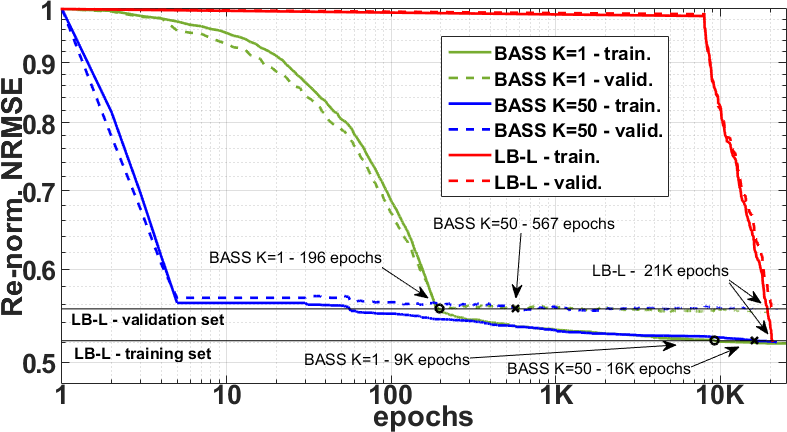
(a)

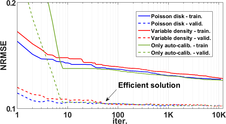
(b)

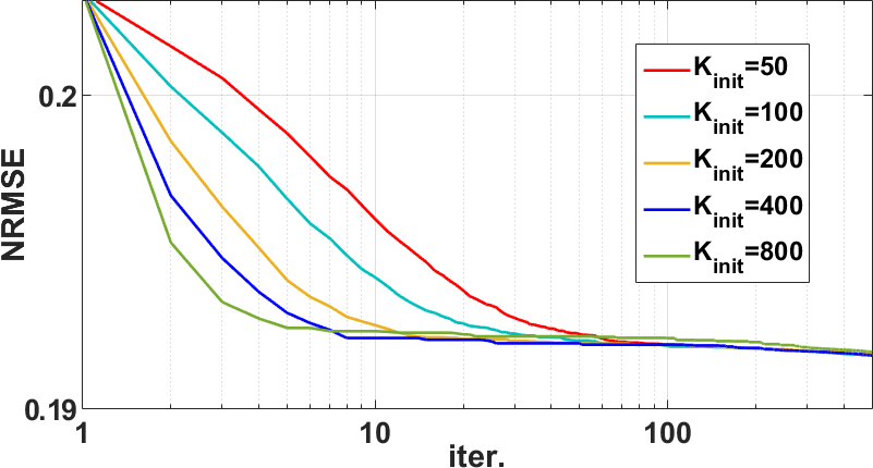
(c)

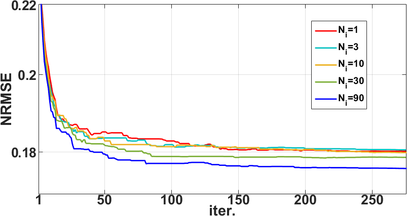
(d)

Figure 2: Convergence curves for BASS. (a) Comparison with the greedy approach LB-L. (b) Comparing various initial SPs. (c) Comparing various $K_{init}$s. (d) Comparing various training sizes.

In Figure 2a we compare BASS with the greedy approach “learning-based lazy” (LB-L)⁴⁹, adapted to the cost function in (2). We used CS-SFD with the reduced-size knee dataset, starting with the auto-calibration area and AF=20. The resulting NRMSEs re-normalized by the initial values, show the difference in computational cost between the approaches. Plots are scaled logarithmically in epochs (in each “epoch” all the images are reconstructed once). BASS (K=1, 196 epochs) found an efficient solution $100$ times faster than LB-L (~21,000 epochs). BASS goes on minimizing the cost function beyond the stopping point of LB-L.

Figure 2b, demonstrates the performance of BASS for various initial SPs (same experimental setup as for Figure 2a, but using AF=15, and $K_{init}$=50). The improvement observable in the validation set ends quickly, at iteration 50 in this example. There is an arrow in the figure pointing to an efficient solution. Such a solution is obtained after a relatively few iterations, during which most of the significant improvement observable with validation data has already happened. Iterating beyond this point essentially leads to marginal improvement, observable only with the training data.

In Figure 2c we see the results of the learning process for the training data according to the parameters $K_{init}$ for CS-LR, AF=20, using the knee dataset, with $N_{i}=30$ and $N_{v}=10$. Note that large $K_{init}$ performs better than small $K_{init}$ in terms of speed of convergence in the beginning of the learning process. Over time, $K$ reduces from $K_{init}$ towards $K=1$.

The importance of large and diverse datasets to generate the learned sampling pattern for the specific class of images is illustrated in Figure 2d, showing the convergence of the learning process with the validation set, in NRMSE. We used training sets of 1, 3, 10, 30, and 90 images. The validation sets were composed of the same 20 images, not used in any of the training sets.

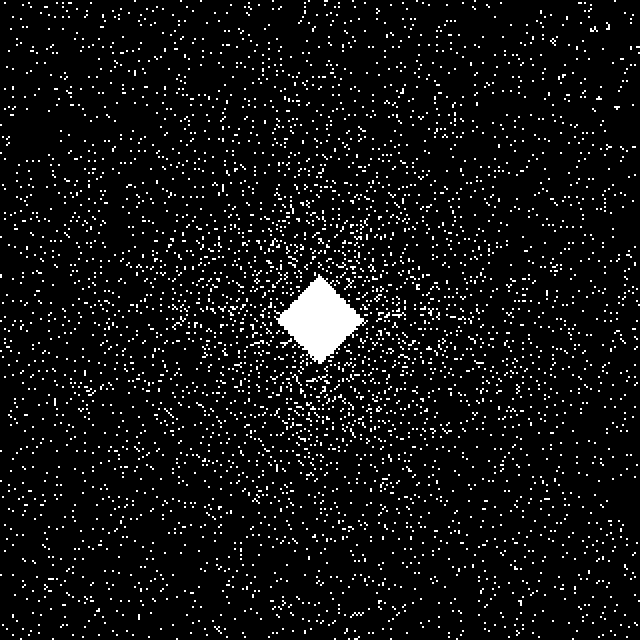
(a)

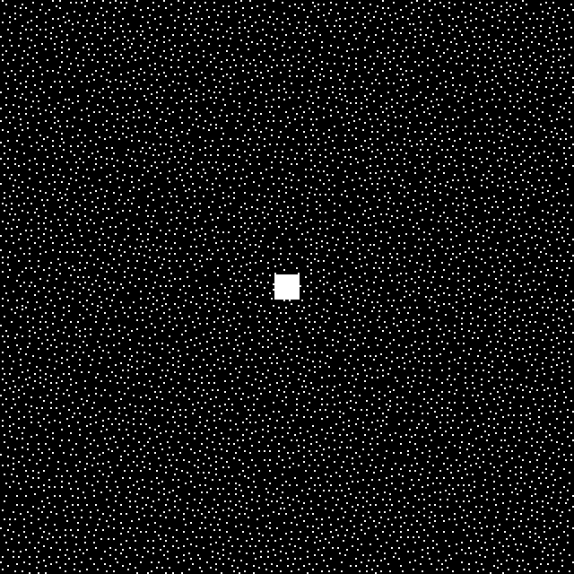
(b)

(c)

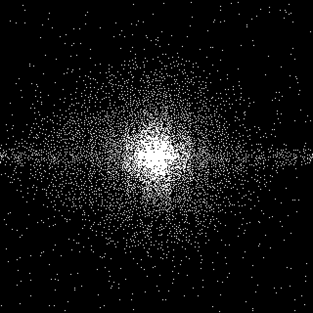
(d)

(e)

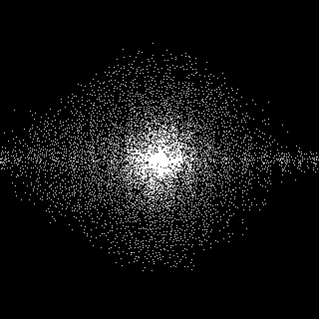
(f)

Figure 3: Efficient solutions produced for P-LORAKS with AF=16 and initial SPs (a) variable density (VD), (b) Poisson disk (PD), and (c) an SP that is empty except for a small central area (CA). The corresponding efficient solutions are the SPs in (d) for VD (NRMSE=0.196), in (e) for PD (NRMSE=0.195), and in (f) for CA (NRMSE=0.194).

The robustness of an efficient solution in the presence of variable initial SP is illustrated in Figure 3. Figure 3a-c show three initial SPs: variable density (VD), Poisson disk (PD), and empty except for a small central area (CA). Using 200 iterations of BASS for P-LORAKS with these initial SPs, corresponding efficient SPs were obtained; shown in Figure 3d-f. There are minor differences among them (less than 1% difference in NRMSE), but the central parts of the SPs are very similar.

4.2 Performance with various reconstruction methods:

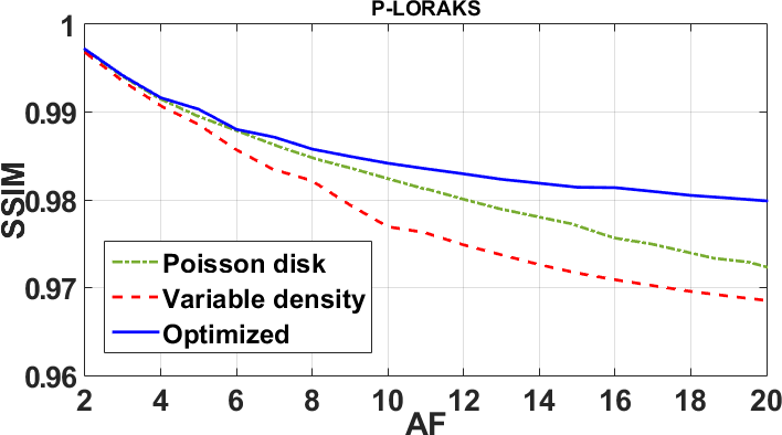
(a)

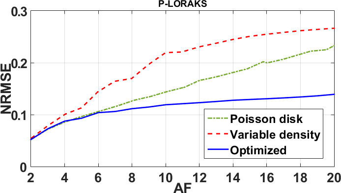
(b)

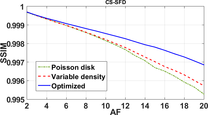
(c)

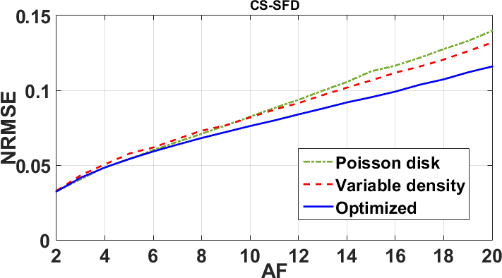
(d)

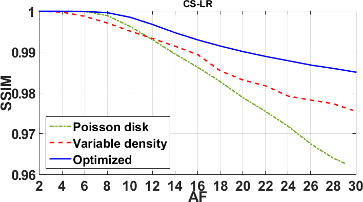
(e)

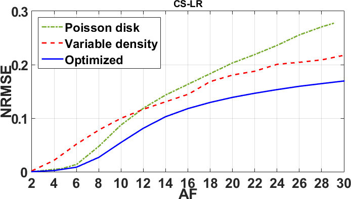
(f)

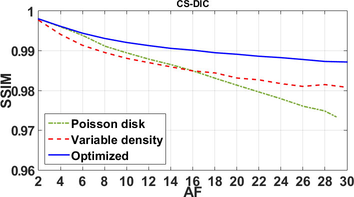
(g)

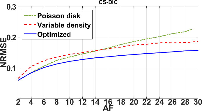
(h)

Figure 4: SSIM (higher is better) and NRMSE (lower is better): (a)-(b) for P-LORAKS, (c)-(d) for CS-SFD, (e)-(f) for CS-LR, and (g)-(h) for CS-DIC, using variable density or Poisson disk SP compared with optimized SP (obtained by BASS) for various AFs. (a)-(d) are for brain dataset and (e)-(h) for knee dataset.

BASS improves both SSIM and NRMSE in image space for fixed AFs when compared with variable density sampling or Poisson disk for the four reconstruction methods. Figures 4a-b show the SSIM and NRMSE obtained by P-LORAKS with brain dataset, compared to variable density, Poisson disk, and the optimized SP. Figures 4c-d show the SSIM and NRMSE obtained by CS-SFD with brain dataset. Figures 4e-f show the SSIM and NRMSE obtained by CS-LR with knee dataset, comparing Poisson disk, variable density, and the optimized SP. Figures 4g-h show the SSIM and NRMSE obtained by CS-DIC with knee dataset. The Poisson disk and variable density SP had their parameters optimized for each reconstruction method and each AF.

(a) FS

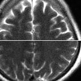
(b) Optimized AF=16

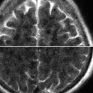
(c) Poisson disk AF=16

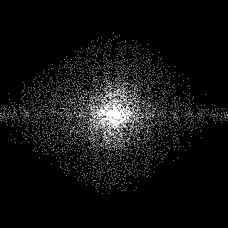
(d) Optimized AF=16

(e) Poisson disk AF=16

(f) FS

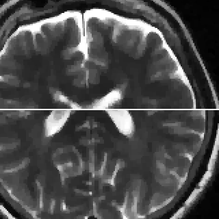
(g) Optimized AF=16

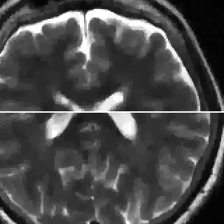
(h) Variable density AF=16

(i) Optimized AF=16

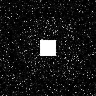
(j) Variable density AF=16

Figure 5: Images of the brain dataset reconstructed with P-LORAKS are shown in (b)-(c), with CS-SFD in (g)-(h) and using fully sampled (FS) data in (a) and (f). Optimized and Poisson disk SPs used with P-LORAKS are shown in (d) and (e) and optimized and variable density SPs used in CS-SFD, with a central-square auto-calibration region, in (i) and (j).

Figure 5 illustrates on the brain dataset how the optimized SPs improve the reconstructed images with P-LORAKS and CS-SFD (for AF=16). The P-LORAKS methods had a visible improvement in SNR, the CS-SFD methods became less smooth with some structures more detailed. Figure 5 also illustrates that optimized SPs are different for the two reconstruction methods, even when using the same images for training.

(a) CS-DIC Poisson disk

(b) CS-DIC Optimized

(c) Poisson disk SP

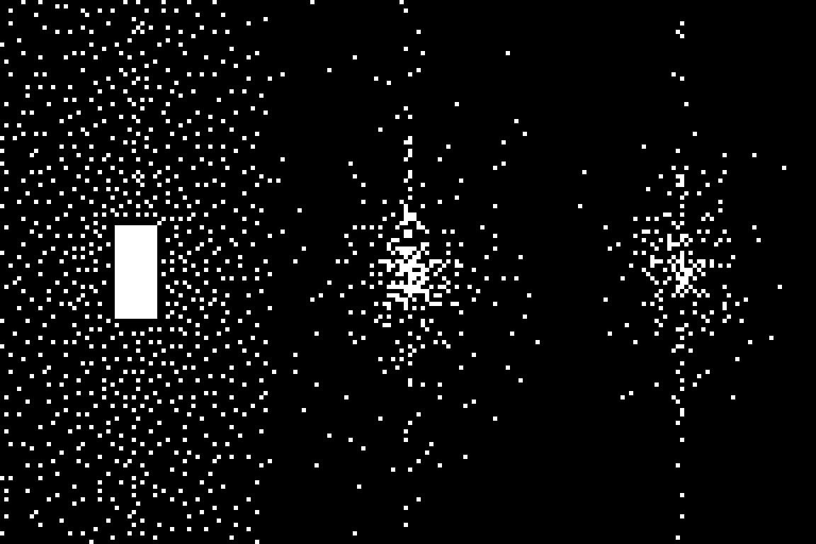
(d) Optimized SP CS-DIC

(e) CS-LR Poisson disk

(f) CS-LR Optimized

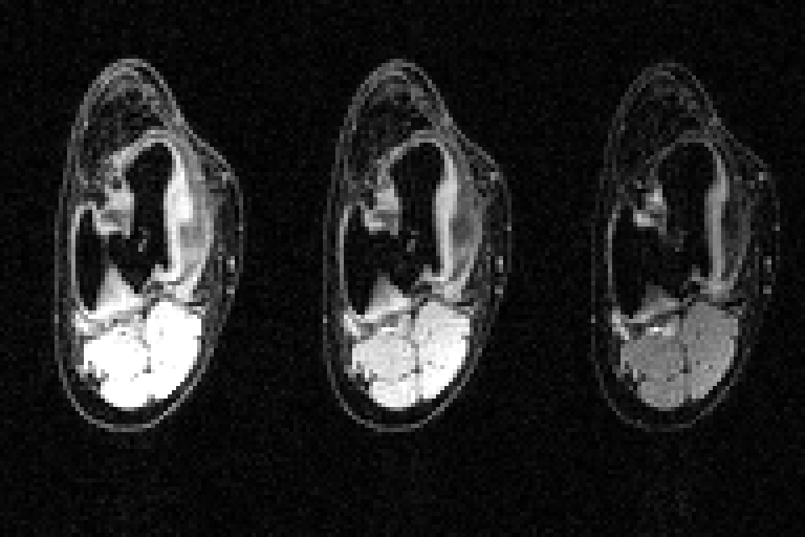
(g) FS

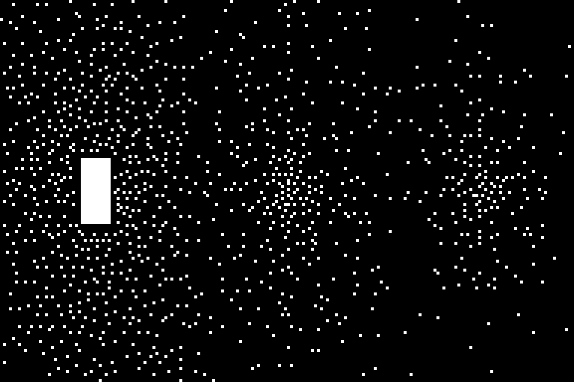
(h) Optimized SP CS-LR

Figure 6: Three frames for different relaxation times of the knee dataset, when AF=24 was used, reconstructed with CS-DIC (a)-(b) and with CS-LR (e)-(f): compare these with the corresponding fully sampled (FS) data in (g). Poisson disk (c) and BASS optimized SPs (d) and (h) are also shown.

In Figure 6, visual results with the knee dataset illustrate the improvement due to using an optimized SP as compared to using the Poisson disk SP, for both CS-LR and CS-DIC. We also see that the optimized SPs are different for the two reconstruction methods. Note that both optimized k-t-space SPs have a different sampling density over time (first, middle, and last time frames are shown), being more densely sampled at the beginning of the relaxation process. The auto-calibration region in the first frame.

4.3 BASS with a different criterion:

We illustrate that our proposed optimization approach is also efficacious with different criteria. In some applications, one may desire the best possible image quality, regardless of k-space measurements. Here we discuss the use of BASS to optimize the SSIM of ⁸¹, an image-domain criterion. For that, the task in (3) of finding the minimizer of $F(\Omega)$ in (2), used in line 10 of the Algorithm 1, is replaced by finding the minimizer in (11), with $g\left(\mathbf{x},\mathbf{y}\right)$ the negative of the SSIM. In Figure 7 we compare the optimization of SSIM with that of NRMSE, using P-LORAKS on the brain dataset, AF=16, starting with the Poisson disk SP.

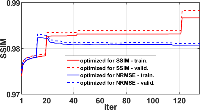
(a)

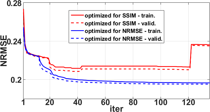
(b)

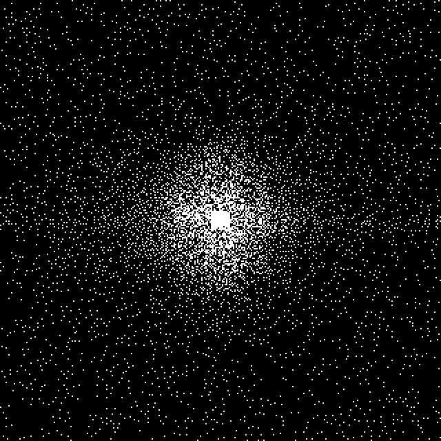
(c)

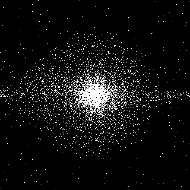
(d)

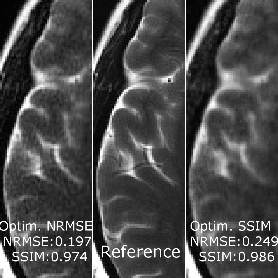
(e)

Figure 7: Comparing BASS in optimizing SSIM and NRMSE. (a) SSIM and (b) NRMSE along the iterations, (c) SP obtained by optimizing SSIM, (d) SP obtained by optimizing NRMSE, and (e) some visual results.

5 Discussion

The proposed approach delivers efficacious sampling patterns for high-resolution or quantitative parallel MRI problems. Compared to previous approaches, as in ^{48, 49, 50, 51, 52}, BASS is able to optimize much larger SPs, using larger datasets, spending less computational time than greedy approaches (Figure 2a). Greedy approaches test considerably more candidates SPs before updating the SP. They are computationally affordable only for 1D undersampling or small SPs.

The proposed approach is effective because it uses a smart selection of new elements in the SP updating process. Candidates that are most likely to reduce the cost function are tried first. The obtained efficient solution may have minor differences depending on the initial SP (Figure 3), but the optimized SPs tend to have the same final quality if more iterations are used (Figure 2b). Adding and removing multiple points at each iteration is beneficial for fast convergence at the initial iterations (Figure 2c).

While the determination of the optimal number of training images is still an open problem, we observed that using a large number of well-distributed images in the training process helps to produce SPs that work better with other unknown images (Figure 2d). The learned SP can be used with new acquisitions of the same anatomy. This also favors the use of fast training algorithms with larger datasets, instead of computationally costly methods (such as greedy approaches) with small datasets.

The cost function in (2) evaluates the error in k-space, not in the image domain. This may not be sufficiently flexible because it does not allow the specification of regions of interest in the image domain. Nevertheless, improvements measured by the image-domain criteria NRMSE and SSIM were observed (Figure 4). In different MRI applications other criteria than (2) may be desired. The proposed algorithm can be used for other criteria, such as the SSIM (Figure 7).

The optimized SP varies with the reconstruction method (Figures 5 and 6) or with the optimization criterion (Figure 7): thus sampling and reconstruction should be matched. This concept of matched sampling-reconstruction indicates that comparing different reconstruction methods with the same SP is not a fair approach, instead each MRI reconstruction method should be compared using its best possible SP. Note that the optimized SP improved the NRMSE by up to 45% in some cases (Figure 4).

The experiments also show that optimizing the SP is more important at higher AFs. As seen in Figure 4, the optimization of the SP flattened the curves of the error over AF, achieving a lower error with the same AF. For example, P-LORAKS with optimized SP at AF=20 obtained the same level of NRMSE as with variable density SP at AF=6, while CS-LR with optimized SP at AF=30 obtained the same level as with Poisson disk SP at AF=16, even after optimizing the parameters used to generate the Poisson disk SP. These indicate that it is possible to double the AF by optimizing the SP. Variable sampling rate over time is advantageous for $\text{T}_{1\rho}$ mapping as seen in ⁸²; it is very interesting that the algorithm learned it, as shown in Figure 6.

Note that regularized algorithms, such as CS methods, may require to estimate, or even optimize, the regularization parameter since the best parameter is unknown a priori. Our approach is to optimize the parameter using the initial SP, and re-optimize it with the learned SP. However, joint optimization of the algorithm parameters and the SP may be a better approach to be investigated in the future. This is important for merging our approach with deep learning reconstruction, where learning sampling and reconstruction happen simultaneously, as recently in ^{53, 54, 55}. That appears to us likely to be the most suitable way for learned reconstruction approaches ^{17, 19, 20, 83}, as well as for classical parametric inverse problems-based reconstructions ^{84, 85, 86}.

The lower computational cost and rapid convergence speed of BASS bring the advantage of learning the optimal SP for various reconstruction methods considering the same anatomy. Thus one can have a better decision on which matched sampling and reconstruction is the most effective for specific anatomy and contrast at the desired AF. Many questions regarding the best way to sample in accelerated MRI can be answered with the help of machine learning algorithms such as BASS. This new learning method is expected to be a key element in making higher AFs available in clinical scanners for translational research.

6 Conclusions

We proposed a data-driven approach for learning the sampling pattern in parallel MRI. It has a low computational cost and converges quickly, enabling the use of large datasets to optimize large sampling patterns, which is important for high-resolution Cartesian 3D-MRI and quantitative and dynamic MRI applications. The approach considers data for specific anatomy and assumes a specific reconstruction method. Our experiments show that the optimized SPs are different for different reconstruction methods, suggesting that matching the sampling to the reconstruction method is important. The approach improves the acceleration factor and helps with finding the best SP for reconstruction methods in various applications of parallel MRI.

References

- 1 Bernstein M, King K, Zhou X. Handbook of MRI pulse sequences. Academic Press; 2004.
- 2 Liang Z P, Lauterbur P C. Principles of magnetic resonance imaging: a signal processing perspective. IEEE Press; 2000.
- 3 Tsao J. Ultrafast imaging: Principles, pitfalls, solutions, and applications. J. Magn. Reson. Imaging. 2010;32(2):252–266.
- 4 Ying L, Liang Z P. Parallel MRI Using Phased Array Coils. IEEE Signal. Proc. Mag.. 2010;27(4):90–98.
- 5 Pruessmann K P. Encoding and reconstruction in parallel MRI. NMR Biomed.. 2006;19(3):288–299.
- 6 Blaimer M, Breuer F, Mueller M, Heidemann R M, Griswold M A, Jakob P M. SMASH, SENSE, PILS, GRAPPA. Top. Magn. Reson. Imaging. 2004;15(4):223–236.
- 7 Feinberg D A, Setsompop K. Ultra-fast MRI of the human brain with simultaneous multi-slice imaging. J. Magn. Reson.. 2013;229:90–100.
- 8 Barth M, Breuer F, Koopmans P J, Norris D G, Poser B A. Simultaneous multislice (SMS) imaging techniques. Magn. Reson. Med.. 2016;75(1):63–81.
- 9 Lustig M, Donoho D L, Pauly J M. Sparse MRI: The application of compressed sensing for rapid MR imaging. Magn. Reson. Med.. 2007;58(6):1182–1195.
- 10 Trzasko J, Manduca A. Highly undersampled magnetic resonance image reconstruction via homotopic -minimization. IEEE Trans. Med. Imag.. 2009;28(1):106–121.
- 11 Lustig M, Donoho D L, Santos J M, Pauly J M. Compressed sensing MRI. IEEE Signal. Proc. Mag.. 2008;25(2):72–82.
- 12 Wang Y. Description of parallel imaging in MRI using multiple coils. Magn. Reson. Med.. 2000;44(3):495–499.
- 13 Wright K L, Hamilton J I, Griswold M A, Gulani V, Seiberlich N. Non-Cartesian parallel imaging reconstruction. J. Magn. Reson. Imaging. 2014;40(5):1022–1040.
- 14 Feng L, Benkert T, Block K T, Sodickson D K, Otazo R, Chandarana H. Compressed sensing for body MRI. J. Magn. Reson. Imaging. 2017;45(4):966–987.
- 15 Lee J A, Verleysen M. Nonlinear dimensionality reduction. Springer Science + Business Media, LCC; 2007.
- 16 Elad M, Figueiredo M A T, Ma Y. On the role of sparse and redundant representations in image processing. Proc. IEEE. 2010;98(6):972–982.
- 17 Jacob M, Mani M P, Ye J C. Structured low-rank algorithms: Theory, magnetic resonance applications, and links to machine learning. IEEE Signal. Proc. Mag.. 2020;37(1):54–68.
- 18 Rubinstein R, Bruckstein A M., Elad M. Dictionaries for sparse representation modeling. Proc. IEEE. 2010;98(6):1045–1057.
- 19 Knoll F, Hammernik K, Zhang C, et al. Deep-learning methods for parallel magnetic resonance imaging reconstruction: A survey of the current approaches, trends, and issues. IEEE Signal. Proc. Mag.. 2020;37(1):128–140.
- 20 Liang D, Cheng J, Ke Z, Ying L. Deep magnetic resonance image reconstruction: Inverse problems meet neural networks. IEEE Signal. Proc. Mag.. 2020;37(1):141–151.
- 21 Candès E J, Romberg J. Sparsity and incoherence in compressive sampling. Inverse Prob.. 2007;23(3):969–985.
- 22 Donoho D L. Compressed sensing. IEEE Trans. Inf. Theory. 2006;52(4):1289–1306.
- 23 Haldar J P, Hernando D, Liang Z P. Compressed-sensing MRI with random encoding. IEEE Trans. Med. Imag.. 2011;30(4):893–903.
- 24 Unser M. Sampling-50 years after Shannon. Proc. IEEE. 2000;88(4):569–587.
- 25 Candès E J, Tao T. Near optimal signal recovery from random projections: Universal encoding strategies?. IEEE Trans. Inf. Theory. 2006;52(12):5406–5425.
- 26 Candès E J, Romberg J K, Tao T. Stable signal recovery from incomplete and inaccurate measurements. Commun. Pure Appl. Math.. 2006;59(8):1207–1223.
- 27 Donoho D L, Elad M, Temlyakov V N. Stable recovery of sparse overcomplete representations in the presence of noise. IEEE Trans. Inf. Theory. 2006;52(1):6–18.
- 28 Elad M, Milanfar P, Rubinstein R. Analysis versus synthesis in signal priors. Inverse Prob.. 2007;23(3):947–968.
- 29 Rudin L I, Osher S, Fatemi E. Nonlinear total variation based noise removal algorithms. Physica D. 1992;60(1-4):259–268.
- 30 Zijlstra F, Viergever M A, Seevinck P R. Evaluation of variable density and data-driven k-space undersampling for compressed sensing magnetic resonance imaging. Invest. Radiol.. 2016;51(6):410–419.
- 31 Boyer C, Chauffert N, Ciuciu P, Kahn J, Weiss P. On the generation of sampling schemes for magnetic resonance imaging. SIAM J. Imag. Sci.. 2016;9(4):2039–2072.
- 32 Cheng J Y, Zhang T, Alley M T, Lustig M, Vasanawala S S, Pauly J M. Variable-density radial view-ordering and sampling for time-optimized 3D Cartesian imaging. In: ISMRM Workshop on Data Sampling and Image Reconstruction; 2013.
- 33 Ahmad R, Xue H, Giri S, Ding Y, Craft J, Simonetti O P. Variable density incoherent spatiotemporal acquisition (VISTA) for highly accelerated cardiac MRI. Magn. Reson. Med.. 2015;74(5):1266–1278.
- 34 Wang Z, Arce G R. Variable density compressed image sampling. IEEE Trans. Image Process.. 2010;19(1):264–270.
- 35 Dunbar D, Humphreys G. A spatial data structure for fast Poisson-disk sample generation. ACM Trans. Graphics. 2006;25(3):503–508.
- 36 Murphy M, Alley M, Demmel J, Keutzer K, Vasanawala S, Lustig M. Fast -SPIRiT compressed sensing parallel imaging MRI: Scalable parallel implementation and clinically feasible runtime. IEEE Trans. Med. Imag.. 2012;31(6):1250–1262.
- 37 Kaldate A, Patre B M, Harsh R, Verma D. MR image reconstruction based on compressed sensing using Poisson sampling pattern. In: Second International Conference on Cognitive Computing and Information Processing (CCIP)IEEE; 2016.
- 38 Knoll F, Clason C, Diwoky C, Stollberger R. Adapted random sampling patterns for accelerated MRI. Magn. Reson. Mater. Phys., Biol. Med.. 2011;24(1):43–50.
- 39 Choi J, Kim H. Implementation of time-efficient adaptive sampling function design for improved undersampled MRI reconstruction. J. Magn. Reson.. 2016;273:47–55.
- 40 Vellagoundar J, Machireddy R R. A robust adaptive sampling method for faster acquisition of MR images. Magn. Reson. Imaging. 2015;33(5):635–643.
- 41 Krishna C, Rajgopal K. Adaptive variable density sampling based on Knapsack problem for fast MRI. In: IEEE International Symposium on Signal Processing and Information Technology (ISSPIT):364–369IEEE; 2015.
- 42 Zhang Y, Peterson B S, Ji G, Dong Z. Energy preserved sampling for compressed sensing MRI. Comput. Math. Methods Med.. 2014;2014:1–12.
- 43 Kim W, Zhou Y, Lyu J, Ying L. Conflict-cost based random sampling design for parallel MRI with low rank constraints. In: Ahmad Fauzia, ed. Compressive Sensing IV, Compressive Sensing IV, vol. 9484: :94840P; 2015.
- 44 Haldar J P, Kim D. OEDIPUS: An experiment design framework for sparsity-constrained MRI. IEEE Trans. Med. Imag.. 2019;38(7):1545–1558.
- 45 Seeger M, Nickisch H, Pohmann R, Schölkopf B. Optimization of k-space trajectories for compressed sensing by Bayesian experimental design. Magn. Reson. Med.. 2010;63(1):116–126.
- 46 Zhao B, Haldar J P, Liao C, et al. Optimal experiment design for magnetic resonance fingerprinting: Cramér-Rao bound meets spin dynamics. IEEE Trans. Med. Imag.. 2019;38(3):844–861.
- 47 Bouhrara M, Spencer R G. Fisher information and Cramér-Rao lower bound for experimental design in parallel imaging. Magn. Reson. Med.. 2018;79(6):3249–3255.
- 48 Gözcü B, Mahabadi R K, Li Y H, et al. Learning-based compressive MRI. IEEE Trans. Med. Imag.. 2018;37(6):1394–1406.
- 49 Gözcü B, Sanchez T, Cevher V. Rethinking sampling in parallel MRI: A data-driven approach. In: European Signal Processing Conference; 2019.
- 50 Sanchez T, Gözcü B, Heeswijk R B, et al. Scalable learning-based sampling optimization for compressive dynamic MRI. In: IEEE International Conference on Acoustics, Speech and Signal Processing:8584–8588IEEE; 2020.
- 51 Liu D D, Liang D, Liu X, Zhang Y T. Under-sampling trajectory design for compressed sensing MRI. In: Annual International Conference of the IEEE Engineering in Medicine and Biology Society:73–76IEEE; 2012.
- 52 Ravishankar S, Bresler Y. Adaptive sampling design for compressed sensing MRI. In: 2011 Annual International Conference of the IEEE Engineering in Medicine and Biology Society, vol. 2011: :3751–3755IEEE; 2011.
- 53 Bahadir C D, Wang A Q, Dalca A V, Sabuncu M R. Deep-Learning-Based Optimization of the Under-Sampling Pattern in MRI. IEEE Trans. Comput. Imag.. 2020;6:1139–1152.
- 54 Aggarwal H K, Jacob M. J-MoDL: Joint Model-Based Deep Learning for Optimized Sampling and Reconstruction. IEEE J. Sel. Topics Signal Process.. 2020;14(6):1151–1162.
- 55 Weiss T, Vedula S, Senouf O, Michailovich O, Zibulevsky M, Bronstein A. Joint Learning of Cartesian under Sampling Andre Construction for Accelerated MRI. In: IEEE International Conference on Acoustics, Speech and Signal Processing:8653–8657IEEE; 2020.
- 56 Broughton R, Coope I, Renaud P, Tappenden R. Determinant and exchange algorithms for observation subset selection. IEEE Trans. Image Process.. 2010;19(9):2437–2443.
- 57 Zhou Z H, Yu Y, Qian C. Evolutionary learning: Advances in theories and algorithms. Singapore: Springer Singapore; 2019.
- 58 Couvreur C, Bresler Y. On the optimality of the backward greedy algorithm for the subset selection problem. SIAM J. Matrix Anal. Appl.. 2000;21(3):797–808.
- 59 Qian C, Yu Y, Zhou Z H. Subset selection by Pareto optimization. In: Advances in Neural Information Processing Systems, vol. 2015: :1774–1782; 2015.
- 60 Qian C, Shi J C, Yu Y, Tang K, Zhou Z H. Subset selection under noise. In: Advances in Neural Information Processing Systems, vol. 2017: :3561–3571; 2017.
- 61 Shin P J, Larson P E Z, Ohliger M A, et al. Calibrationless parallel imaging reconstruction based on structured low-rank matrix completion. Magn. Reson. Med.. 2014;72(4):959–970.
- 62 Haldar J P. Low-rank modeling of local k-space neighborhoods (LORAKS) for constrained MRI. IEEE Trans. Med. Imag.. 2014;33(3):668–681.
- 63 Ongie G, Jacob M. A fast algorithm for convolutional structured low-rank matrix recovery. IEEE Trans. Comput. Imag.. 2017;3(4):535–550.
- 64 Jin K H, Lee D, Ye J C. A general framework for compressed sensing and parallel MRI using annihilating filter based low-rank Hankel matrix. IEEE Trans. Comput. Imag.. 2016;2(4):480–495.
- 65 Haldar J P, Zhuo J. P-LORAKS: Low-rank modeling of local k-space neighborhoods with parallel imaging data. Magn. Reson. Med.. 2016;75(4):1499–1514.
- 66 Zibetti M V W, Sharafi A, Otazo R, Regatte R R. Accelerating 3D-T1 mapping of cartilage using compressed sensing with different sparse and low rank models. Magn. Reson. Med.. 2018;80(4):1475–1491.
- 67 Zibetti M V W, Herman G T, Regatte R R. Data-driven design of the sampling pattern for compressed sensing and low rank reconstructions on parallel MRI of human knee joint. In: ISMRM Workshop on Data Sampling and Image Reconstruction; 2020.
- 68 Pruessmann K P, Weiger M, Scheidegger M B, Boesiger P. SENSE: Sensitivity encoding for fast MRI. Magn. Reson. Med.. 1999;42(5):952–962.
- 69 Zibetti M V W, Baboli R, Chang G, Otazo R, Regatte R R. Rapid compositional mapping of knee cartilage with compressed sensing MRI. J. Magn. Reson. Imaging. 2018;48(5):1185–1198.
- 70 Uecker M, Lai P, Murphy M J, et al. ESPIRiT-an eigenvalue approach to autocalibrating parallel MRI: Where SENSE meets GRAPPA. Magn. Reson. Med.. 2014;71(3):990–1001.
- 71 Walsh D O, Gmitro A F, Marcellin M W. Adaptive reconstruction of phased array MR imagery. Magn. Reson. Med.. 2000;43(5):682–690.
- 72 Roemer P B, Edelstein W A, Hayes C E, Souza S P, Mueller O M. The NMR phased array. Magn. Reson. Med.. 1990;16(2):192–225.
- 73 Liu B, Zou Y M, Ying L. SparseSENSE: Application of compressed sensing in parallel MRI. In: International Conference on Technology and Applications in Biomedicine, vol. 2: :127–130IEEE; 2008.
- 74 Liang D, Liu B, Wang J, Ying L. Accelerating SENSE using compressed sensing. Magn. Reson. Med.. 2009;62(6):1574–1584.
- 75 Haldar J P. Autocalibrated LORAKS for fast constrained MRI reconstruction. In: IEEE International Symposium on Biomedical Imaging:910–913IEEE; 2015.
- 76 Liang Z P. Spatiotemporal imaging with partially separable functions. In: IEEE International Symposium on Biomedical Imaging, vol. 2: :988–991IEEE; 2007.
- 77 Doneva M, Börnert P, Eggers H, Stehning C, Sénégas J, Mertins A. Compressed sensing reconstruction for magnetic resonance parameter mapping. Magn. Reson. Med.. 2010;64(4):1114–1120.
- 78 Zibetti M V W, Helou E S, Sharafi A, Regatte R R. Fast multicomponent 3D-T1 relaxometry. NMR Biomed.. 2020;:e4318.
- 79 Zibetti M V W, Helou E S, Regatte R R, Herman G T. Monotone FISTA with variable acceleration for compressed sensing magnetic resonance imaging. IEEE Trans. Comput. Imag.. 2019;5(1):109–119.
- 80 Knoll F, Zbontar J, Sriram A, et al. fastMRI: A Publicly Available Raw k-Space and DICOM Dataset of Knee Images for Accelerated MR Image Reconstruction Using Machine Learning. Radiology: Artificial Intelligence. 2020;2(1):e190007.
- 81 Wang Z, Bovik A C, Sheikh H R, Simoncelli E P. Image quality assessment: from error visibility to structural similarity.. IEEE Trans. Image Process.. 2004;13(4):600–612.
- 82 Zhu Y, Liu Y, Ying L, Liu X, Zheng H, Liang D. Bio-SCOPE: fast biexponential T1 mapping of the brain using signal-compensated low-rank plus sparse matrix decomposition. Magn. Reson. Med.. 2020;83(6):2092–2106.
- 83 Wen B, Ravishankar S, Pfister L, Bresler Y. Transform learning for magnetic resonance image reconstruction: From model-based learning to building neural networks. IEEE Signal. Proc. Mag.. 2020;37(1):41–53.
- 84 Fessler J A. Optimization methods for magnetic resonance image reconstruction: Key models and optimization algorithms. IEEE Signal. Proc. Mag.. 2020;37(1):33–40.
- 85 Doneva M. Mathematical models for magnetic resonance imaging reconstruction: An overview of the approaches, problems, and future research areas. IEEE Signal. Proc. Mag.. 2020;37(1):24–32.
- 86 Sandino C M, Cheng J Y, Chen F, Mardani M, Pauly J M, Vasanawala S S. Compressed sensing: From research to clinical practice with deep neural networks: Shortening scan times for magnetic resonance imaging. IEEE Signal. Proc. Mag.. 2020;37(1):117–127.