Kernel Mean Embedding of Probability Measures and its Applications to Functional Data Analysis

Abstract

This study intends to introduce kernel mean embedding of probability measures over infinite-dimensional separable Hilbert spaces induced by functional response statistical models. The embedded function represents the concentration of probability measures in small open neighborhoods, which identifies a pseudo-likelihood and fosters a rich framework for statistical inference. Utilizing Maximum Mean Discrepancy, we devise new tests in functional response models. The performance of new derived tests is evaluated against competitors in three major problems in functional data analysis including function-on-scalar regression, functional one-way ANOVA, and equality of covariance operators.

1 Introduction

Functional response models are among the major problems in the context of Functional Data Analysis. A fundamental issue in dealing with functional response statistical models arises due to the lack of practical frameworks on characterizing probability measure on function spaces. This is mainly a consequence of the tremendous gap on how we present probability measures in finite-dimensional and infinite-dimensional spaces.

A useful property of finite-dimensional spaces is the existence of a locally finite, strictly positive, and translation invariant measure like Lebesgue or counting measure, which makes it easy to take advantage of probability measures directly in the statistical inference. Fitting a statistical model, and estimating parameters, hypothesis testing, deriving confidence regions and developing goodness of fit indices, all can be applied by integrating distribution or conditional distribution of response variables as a presumption into statistical procedures.

Sporadic efforts have been gone into approximating or representing probability measures on infinite-dimensional spaces. Let $\mathbb{H}$ be a separable infinite-dimensional Hilbert space and $X$ be a $\mathbb{H}$-valued random element with finite second moment and covariance operator $C$. Delaigle and Hall [5] approximated probability of $B_{r}\left(x\right)=\{\parallel X-x\parallel<r\}$ by the surrogate density of a finite-dimensional approximated version of $X$, obtained by projecting the random element $X$ into a space spanned by first few eigenfunctions of $C$ with largest eigenvalues. The approximated small-ball probability is on the basis of Karhunen-Loève expansion and putting an extra assumption that the component scores are independent. The precision of this approximation depends on the volume of ball and probability measure itself.

Let $\mathcal{I}$ be a compact subset of $\mathbb{R}$ such as closed interval $[0,1]$ and $X$ be a zero mean $L^{2}\left[\mathcal{I}\right]$-valued random element with finite second moment and Karhunen-Loève expansion $X=\sum_{j\geq 1}\lambda_{j}^{1/2}X_{j}\psi_{j}$, in which $X_{j}=\lambda_{j}^{-1/2}\langle X,\psi_{j}\rangle$ and $\left\{\lambda_{j},\psi_{j}\right\}_{j\geq 1}$ is the eigensystem of covariance operator $C$. Suppose that the distribution of $X_{j}$ is absolutely continuous with respect to the Lebesgue measure with density $f_{j}$. Approximation of the logarithm of $p\left(x\,|\,r\right)=P\left(B_{r}\left(x\right)\right)=P\left(\{\parallel X-x\parallel<r\}\right)$ given by Delaigle and Hall [5] is

$$\log p(x\,|\,r)=C_{1}(h,\left\{\lambda_{j}\right\}_{j\geq 1})+\sum_{j=1}^{h}\log f_{j}(x_{j})+o(h),$$

in which $x_{j}=\left\langle x,\psi_{j}\right\rangle$, and $h$ is the number of components that depends on $r$ and tends to infinity as $r$ declines to zero. $C_{1}\left(\cdot\right)$ depends only on size of the ball and sequence of eigenvalues, though the quantity $o(h)$ as the precision of approximation depends on $P$.

The quantity $h^{-1}\sum_{j=1}^{h}\log f_{j}(x_{j})$ is called log-density by Delaigle and Hall [5]. A serious concern with this approximation is its precision, which depends on the probability measure itself. Accordingly, it can not be employed to compare small-ball probability in a family of probability measures. For example, in the case of estimating the parameters in a functional response regression model, the induced probability measure varies with different choices of parameters. Thus this approximation can not be employed for parameter estimation and comparing the goodness of fit of different regression models.

Another work in representing probability measures on a general separable Hilbert space $\mathbb{H}$ presented by Lin et al. [17]. They constructed a dense subspace of $\mathbb{H}$ called Mixture Inner Product Space (MIPS), which is the union of a countable collection of finite-dimensional subspaces of $\mathbb{H}$. An approximating version of the given $\mathbb{H}$-valued random element lies in this subspace, which in consequence, lies in a finite-dimensional subspace of $\mathbb{H}$ according to a given discrete distribution. They defined a base measure on the MIPS, which is not translation-invariant, and introduced density functions for the MIPS-valued random elements.

Absence of a proper method in representing probability measures over infinite-dimensional spaces caused severe problems to statistical inference. To make it clear, as an example Greven et al. [9] developed a general framework for functional additive mixed-effect regression models. They considered a log-likelihood function by summing up the log-likelihood of response functions $Y_{i}$ at a grid of time-points $t_{id},~{}d=1,\ldots,D_{i}$, assuming $Y_{i}\left(t_{id}\right)$ to be independent within the grid of time-points. A simulation study by Kokoszka and Reimherr [16] revealed the weak performance of the proposed framework in statistical hypothesis testing in a simple Gaussian Function-on-Scalar linear regression problem.

Currently, MLE and other density-based methods are out of reach in the context of functional response models. In this study, we follow a different path by identifying probability measures with their kernel mean functions and introduce a framework for statistical inference in infinite-dimensional spaces. A promising fact about the kernel mean functions, which is shown in this paper, is their ability to reflect the concentration of probability measures in small open neighborhoods, where unlike the approach of Delaigle and Hall [5] is comparable among different probability measures. This property of kernel mean function motivates us to make use of it in fitting statistical models and introducing new statistical tests in the context of functional data analysis.

This paper is organized as follows: In Section 2, kernel mean embedding of probability measures over infinite-dimensional separable Hilbert spaces is discussed. In Section 3 the Maximum Kernel Mean estimation method is introduced and estimators for Gaussian Response Regression models are derived. In Section 4, new statistical tests are developed for three major problems in functional data analysis and their performance evaluated using simulation studies. Section 5 has been devoted to discussion and conclusion. Major proofs are aggregated in the appendix.

2 Kernel mean embedding of probability measures

We summarize the basics of kernel mean embedding. See Muandet et al. [20] for a general reference. Let $(\mathbb{H},B\left(\mathbb{H}\right),P)$ be a probability measure space. Throughout this study $\mathbb{H}$ is an infinite-dimensional separable Hilbert space equipped with inner product $\langle\cdot,\cdot\rangle_{\mathbb{H}}$. A function $k$ : $\mathbb{H}\times\mathbb{H}\to\mathbb{R}$ is a positive definite kernel if it is symmetric, i.e., $k(x,y)=k(y,x)$ and $\sum_{i=1}^{n}a_{i}a_{j}k(x_{i},x_{j})\geq 0$ for all $n\in\mathbb{N}$ and $a_{i}\in\mathbb{R}$ and $x_{i}\in\mathbb{H}$. $k$ is strictly positive definite if equality implies $a_{1}=a_{2}=\ldots=a_{n}=0$. $k$ is said to be integrally strictly positive definite if $\int k(x,y)\mu(dx)\mu(dy)>0$ for any non-zero finite signed measure $\mu$ defined over $(\mathbb{H},B\left(\mathbb{H}\right))$. Any integrally strictly positive definite kernel is strictly positive definite while the converse is not true [26]. A positive definite kernel induces a Hilbert space of functions over $\mathbb{H}$, which is called Reproducing Kernel Hilbert Space (RKHS) and equals to $\mathcal{H}_{k}=\overline{span}\{k(x,\cdot);x\in\mathbb{H}\}$ with inner product

$$\langle\sum_{i\geq 1}a_{i}k(x_{i},\cdot),\sum_{i\geq 1}b_{i}k(y_{i},\cdot)\rangle_{\mathcal{H}_{k}}=\sum_{i\geq 1}\sum_{j\geq 1}a_{i}b_{j}k(x_{i},y_{j}).$$

For each $f\in\mathcal{H}_{k}$ and $x\in\mathbb{H}$ we have $f(x)=\langle f,k(.,x)\rangle_{\mathcal{H}_{k}}$, which is the reproducing property of kernel $k$. A strictly positive definite kernel $k$ is said to be characteristic for a family of measures $\mathscr{P}$ if the map

$$m:\mathscr{P}\rightarrow\mathcal{H}_{k}\qquad P\mapsto\int k(x,.)P(dx)$$

is injective. If $\mathbb{E}_{P}(\sqrt{k(X,X)})<\infty$ then $m_{P}(\cdot):=(m(P))(\cdot)$ exists in $\mathcal{H}_{k}$ [20], and the function $m_{P}(\cdot)=\int k(x,\cdot)P(dx)$ is called kernel mean function. Moreover, for any $f\in\mathcal{H}_{k}$ we have $\mathbb{E}_{P}[f(X)]=\langle f,m_{P}\rangle_{\mathcal{H}_{k}}$ [25]. Thus, if kernel $k$ is characteristic then every probability measure defined over $(\mathbb{H},\Sigma)$ is uniquely identified by an element $m_{P}$ of $\mathcal{H}_{k}$ and Maximum Mean Discrepancy (MMD) defined as

$$\text{MMD}(\mathcal{H}_{k},\mathbb{P},\mathbb{Q}) =\sup_{f\in\mathcal{H}_{k},\left\|f\right\|_{\mathcal{H}_{k}}\leq 1}\left\{\int f(x)\mathbb{P}(dx)-\int f(x)\mathbb{Q}(dx)\right\}$$

$$=\sup_{f\in\mathcal{H}_{k},\left\|f\right\|_{\mathcal{H}_{k}}\leq 1}\left\langle f,m_{\mathbb{P}}-m_{\mathbb{Q}}\right\rangle=\left\|m_{\mathbb{P}}-m_{\mathbb{Q}}\right\|_{\mathcal{H}_{k}},$$ (1)

is a metric on the family of measures $\mathscr{P}$ over $\mathbb{H}$ [20].

A similar quantity called Ball divergence is proposed by Pan et al. [22] to distinguish probability measures defined over separable Banach spaces. For the case of infinite-dimensional spaces, Ball divergence distinguishes two probability measures if at least one of them possesses a full support, that is, $\text{Supp}\left(P\right)=\mathbb{H}$. They employed Ball divergence for a two-sample test, which according to their simulation results, the performance of both MMD and Ball divergence are close and superior to other tests.

Kernel mean functions can also be used to reflect the concentration of probability measures in small-balls, if the kernel function is translation-invariant. A positive definite kernel $k$ is called translation-invariant if $k(x,y)=\psi(x-y)$ for some positive definite function $\psi$. Gaussian kernel $e^{-\sigma\parallel x-y\parallel_{\mathbb{H}}^{2}}$ and Laplace kernel $e^{-\sigma\parallel x-y\parallel_{\mathbb{H}}}$ are such kernels. If we choose a continuous characteristic kernel that is bounded and translation-invariant, then the kernel mean function $m_{P}$ can be employed to represent the concentration of probability measure in different points of Hilbert space $\mathbb{H}$. for example, consider

$$m_{p}(x)={\displaystyle\int\limits_{\mathbb{H}}e^{-\sigma\left\|x-y\right\|_{\mathbb{H}}^{2}}P(dy)}.$$

If $m_{P}(\cdot)$ has an explicit form for a family of probability measures then $m_{P}(\cdot)$ can be employed to study and compare different probability measures. For example, if $m_{P}(x_{1})>m_{P}(x_{2})$ then it could be concluded that the concentration of probability measure $P$ around the point $x_{1}$ is higher than $x_{2}$, and if for given two probability measures $P_{1}$ and $P_{2}$ we had $m_{P_{1}}(x)>m_{P_{2}}(x)$ then we conclude that the concentration of probability measure $P_{1}$ around the point $x$ is higher than that of probability measure $P_{2}$. This property of kernel mean functions makes them a good candidate to represent probability measures in infinite-dimensional spaces.

The representation property of probability measures by kernel mean functions is addressed in the next theorem and corollary. Proofs are provided in the appendix.

Theorem 1.

Let $P_{1}$ and $P_{2}$ be two probability measures on a separable Hilbert space $\mathbb{H}$ over the field $\mathbb{R}$. Let $\psi:\mathbb{R^{+}}\rightarrow\left[0,1\right]$ be a bounded continuous, strictly decreasing and positive definite function e.g. $\psi(t)=e^{-t^{2}}$, such that $k(x,y)=\psi(\left\|x-y\right\|_{\mathbb{H}})$ is a translation-invariant characteristic kernel, and let $m_{P_{1}}(\cdot)$ and $m_{P_{2}}(\cdot)$ be the kernel mean embedding of $P_{1}$ and $P_{2}$, respectively, for the kernel $k\left(\cdot,\cdot\right)$. If $m_{P_{2}}(y)>m_{P_{1}}(y)$ for a given $y\in\mathbb{H}$, then there exists an open ball $B_{r}(y)$ such that $P_{2}\left(B_{r}(y)\right)>P_{1}\left(B_{r}(y)\right)$, and $r$ depends only on difference $m_{P_{2}}(y)-m_{P_{1}}(y)$ and the characteristic kernel itself.

Corollary 2.

Let $P$ be a probability measure on a separable Hilbert space $\mathbb{H}$ over the field $\mathbb{R}$. Let $\psi:\mathbb{R^{+}}\rightarrow\left[0,1\right]$ be a bounded continuous, strictly decreasing and positive definite function e.g. $\psi(t)=e^{-t^{2}}$, such that $k(x,y)=\psi(\left\|x-y\right\|_{\mathbb{H}})$ is a translation-invariant characteristic kernel, and let $m_{p}(\cdot)$ be the kernel mean embedding of $P$ for the kernel $k\left(\cdot,\cdot\right)$. If $m_{P}(y_{2})>m_{P}(y_{1})$ for some $y_{1},y_{2}\in\mathbb{H}$, then there exist open balls of the same size $B_{r}(y_{1})$ and $B_{r}(y_{2})$ such that $P\left(B_{r}(y_{2})\right)>P\left(B_{r}(y_{1})\right)$, and $r$ depends only on difference $m_{P}(y_{2})-m_{P}(y_{1})$ and the characteristic kernel itself.

Kernel Mean Embedding of probability measures also has a connection with kernel scoring rules. Proper Scoring Rules are well-established instruments with applications in assessing probability models [7]. The following definition is borrowed from Steinwart and Ziegel [28] and adapted to our context. In the following definition, $c_{00}$ is the infinite-dimensional inner product space of sequences vanishing at infinity, which is a dense subspace of $\ell_{2}$.

Definition 3.

Let $\mathbb{X}$ be an arbitrary measurable space. Here it may be considered to be either the separable Hilbert space $\ell_{2}$ or the separable inner product space $c_{00}$, and let $\mathcal{M}_{1}\left(\mathbb{X}\right)$ be the space of probability measures on $\mathbb{X}$. For $\mathcal{P}\subseteq\mathcal{M}_{1}\left(\mathbb{X}\right)$, a scoring rule is defined as a function $S:\mathcal{P}\times\mathbb{X}\to\left[-\infty,\infty\right]$ such that the integral $\int_{\mathbb{X}}S\left(P,x\right)Q\left(dx\right)$ exists for all $P,Q\in\mathcal{P}$. The scoring rule is proper if

$$\int_{\mathbb{X}}S\left(P,x\right)P\left(dx\right)\leq\int_{\mathbb{X}}S\left(Q,dx\right)P\left(dx\right),\quad\forall P,Q\in\mathcal{P}$$

and is called strictly proper if the equality implies $P=Q$.

Kernel scores are a general class of proper scoring rules, in which the scoring rule is generated by a symmetric positive definite kernel $k:\mathbb{X}\times\mathbb{X}\to\mathbb{R}$ by

$$S_{k}\left(P,x\right):= -\int k\left(\omega,x\right)P\left(d\omega\right)+\frac{1}{2}\int\int k\left(\omega,\omega^{\prime}\right)P\left(d\omega\right)P\left(d\omega^{\prime}\right)$$

$$= -m_{p}\left(x\right)+\frac{1}{2}\left\|m_{P}\right\|^{2}.$$ (2)

The Maximum Mean Discrepancy distance between $P,Q\in\mathcal{P}$ satisfies

$$\left\|m_{P}-m_{Q}\right\|_{\mathcal{H}_{k}}^{2}=2\left(\int S_{k}\left(Q,x\right)P\left(dx\right)-\int S_{k}\left(P,x\right)P\left(dx\right)\right).$$ (3)

If $k$ is bounded then $\mathcal{P}=\mathcal{M}_{1}\left(\mathbb{X}\right)$ [28]. In effect, a kernel score rule $S_{k}$ is a strictly proper scoring rule if and only if kernel mean embedding is injective or $k$ to be characteristic.

There are a plethora of studies on the different class of characteristic kernels over locally compact spaces. For example, Steinwart [27] proved that Gaussian kernel is characteristic on compact sets, Sriperumbudur et al. [26, Theorem 9] showed that Gaussian kernel is characteristic on the whole space $\mathbb{R}^{d}$, and Simon-Gabriel and Schölkopf [24] studied the connection between various concepts of kernels such as universality, characteristic and positive definiteness of kernels.

Given a separable Hilbert space $\mathbb{H}$, any integrally strictly positive definite kernel is characteristic [26, Theorem 7], however, it is not clear which kernels are integrally strictly positive definite over infinite-dimensional separable Hilbert spaces. To the best of our knowledge, there is no study on existence and construction of characteristic kernels for infinite-dimensional spaces. The following two theorems, proofs of which are provided in Appendix, try to tackle this problem. In Theorem 4, the result of Steinwart and Ziegel [28, Threorem 3.14] is used to show the existence of a continuous characteristic kernel for infinite-dimensional separable Hilbert spaces, and Theorem 5 shows that Gaussian kernel is characteristic for $c_{00}$, the infinite-dimensional inner product space of sequences vanishing at infinity, which is dense in $\ell_{2}$.

Theorem 4.

Let $\mathbb{H}$ be an infinite-dimensional separable Hilbert space. There exists a continuous characteristic kernel on $\mathbb{H}$.

Theorem 5.

Let $c_{00}$ be the space of eventually zero sequences in $\mathbb{R}^{\infty}$. The Gaussian kernel defined as $k\left(x,y\right)=e^{-\sigma\left\|x-y\right\|_{2}^{2}}$ is characteristic on $c_{00}$.

Beside what are presented in Theorem 4 and Theorem 5, we show in Proposition 6 that Gaussian kernel is characteristic for the family of Gaussian probability measures over $\mathbb{H}$.

3 Maximum Kernel Mean Estimation

In the context of multivariate statistics, the density function is considered as one of the most ubiquitous tools in statistical inference. Density is a non-negative function, which represents the amount of probability mass in a point or concentration of probability measure in a very small neighborhood. Typically a nominated family of probability measures is presented by the corresponding family of densities, and the aim is to choose a density from this family, which is the most likely one that generates a set of observations obtained by a probability-based survey sample. The aforementioned family of probability measures usually parameterized by a parameter $\theta$ taking value either in a subset $\Theta$ of a finite-dimensional or infinite-dimensional space.

Suppose that $\left\{P_{\theta},~{}\theta\in\Theta\right\}$ is a nominated family of probability measures indexed by $\theta$. The idea behind MLE is as follows: Suppose we randomly survey the population according to a sampling method and the result is an observation $y$. If $\theta$ is unknown, an estimation of $\theta$ is one for which $P_{\theta}$ is the most likely generator of $y$. If the density function $f_{\theta}=dP_{\theta}/d\lambda$ exists, we seek for a $\theta$ for which $f_{\theta}(x)$ is of maximum value.

What makes a density function suitable for this kind of inference is the base measure $\lambda$ where the density is defined relative to it. A counting measure or Lebesgue measure are suitable options in finite-dimensional spaces. These base measures are positive, locally finite and translation invariant and a nontrivial measure with these properties does not exist in an infinite-dimensional separable Hilbert space [6].

Employing the kernel mean function, we can introduce a rather similar idea to likelihood-based estimation in infinite-dimensional spaces. Suppose $k$ is a bounded, continuous, and translation-invariant characteristic kernel as described in Theorem 1, such as Gaussian kernel $k(x,y)=e^{-\sigma\parallel x-y\parallel_{\mathbb{H}}^{2}}$ for a fixed $\sigma>0$. The kernel mean function $m_{P}(\cdot)$ is a bounded function over $\mathbb{H}$ which reflects the concentration of $P$ on a small neighborhood of $y\in\mathbb{H}$. Consider the family of probability measures $M=\{P_{\theta},~{}\theta\in\Theta\}$ and its counterpart family of kernel mean functions $\{m_{P_{\theta}}(.);\>\theta\in\Theta\}$. Assume that $\theta$ is unknown and the endeavor is to estimate it through an observed random sample $y$ from the population. Again the aim is to pick a $\widehat{\theta}\in\Theta$ such that $P_{\hat{\theta}}$ is the most likely generator of $y$. Thus, it seems possible to estimate $\theta$ by $\widehat{\theta}=\sup_{\theta\in\Theta}m_{P_{\theta}}(y)$.

In this section, we derive the kernel mean embedding of probability measures induced by Functional response models, and we show how parameter estimation and hypothesis testing are capable in this framework.

3.1 Kernel Mean Embedding of Gaussian Probability Measure

The assumption of Gaussianity is prevalent and fundamental to many statistical problems in the context of functional data analysis, including functional response regressions, functional one-way ANOVA, and testing for homogeneity of covariance operators. In this regard, it is desirable to study the kernel mean embedding of Gaussian probability measures induced by these category of models.

Let $\mathbb{H}$ be an arbitrary infinite-dimensional separable Hilbert Space. An $\mathbb{H}$-valued random element is said to be a Gaussian random element with the mean function $\mu$ and covariance operator $C$, for any $a\in\mathbb{H}$, we have $\left\langle a,X\right\rangle\sim N\left(\left\langle a,\mu\right\rangle,\left\langle Ca,a\right\rangle\right)$. A Gaussian random element has a finite second moment, and its covariance operator is trace class [18]. Let $\left(\lambda_{i},\psi_{i}\right)_{i\geq 1}$ be the eigensystem of $C$ and $\mathbb{H}$ be an arbitrary function space such as $L^{2}[0,1]$, then the kernel of integral operator $C$ admits the decomposition $k_{C}(s,t)=\sum_{j\geq 1}\lambda_{j}\psi_{j}(s)\psi_{j}(t)=Cov\left[X(s),X(t)\right]$ [14]. Kernel mean function of the Gaussian family of probability measures with mean $\mu$ and covariance operator $C$ and its uniqueness is given in the following proposition and is proved in the appendix.

Proposition 6.

Let $Y\sim\mathcal{N}\left(\mu,C\right)$ i.e. $\left\langle a,Y\right\rangle\sim\mathcal{N}\left(\left\langle a,\mu\right\rangle,\left\langle Ca,a\right\rangle\right)$ then for a Gaussian kernel,

$$m_{P}(x) =\int_{\mathbb{H}}e^{-\sigma\left\|x-y\right\|_{\mathbb{H}}^{2}}\mathcal{N}\left(\mu,C\right)\left(dy\right)=\left|I+2\sigma C\right|^{-1/2}e^{-\sigma\left\langle\left(I+2\sigma C\right)^{-1}\left(x-\mu\right),\left(x-\mu\right)\right\rangle},$$

the kernel mean embedding is injective and

$$\left\|m_{P}\right\|_{\mathcal{H}_{k}}^{2} =\left|I+4\sigma C\right|^{-{1}/{2}}.$$

Consider a random sample $Y_{i}\in L^{2}[0,1],~{}i=1,\ldots,n$ of independent and identically random elements with distribution $\mathcal{N}\left(\mu,C\right)$ . By choosing a suitable characteristic kernel for the product space $\left(L^{2}[0,1]\right)^{n}$, kernel mean embedding of the induced probability measure by the random sample $\left\{Y_{i}\right\}$ i.e. $\otimes_{i=1}^{n}\mathcal{N}\left(\mu,C\right)$ can be computed. Let $k$ be the Gaussian kernel, then according to the following theorem, which is proved in the appendix, $\prod_{i=1}^{n}k(\cdot,\cdot)$ and $\sum_{i=1}^{n}k(\cdot,\cdot)$ are characteristic kernels for the family of product measures on $\left(L^{2}[0,1]\right)^{n}$.

Proposition 7.

Let $k\left(\cdot,\cdot\right)$ be a characteristic kernel defined over a separable Hilbert space $\mathbb{H}$, then product-kernel

$$k_{P}(\cdot,\cdot):\mathbb{H}^{n}\times\mathbb{H}^{n}\longrightarrow\mathbb{R}\quad\quad\left(\left\{x_{i}\right\},\left\{y_{i}\right\}\right)\mapsto\prod_{i=1}^{n}k(x_{i},y_{i})$$

and sum-kernel

$$k_{S}(\cdot,\cdot):\mathbb{H}^{n}\times\mathbb{H}^{n}\longrightarrow\mathbb{R}\quad\left(\left\{x_{i}\right\},\left\{y_{i}\right\}\right)\mapsto\sum_{i=1}^{n}k(x_{i},y_{i})$$

are two characteristic kernels for the family of product probability measures $\mathscr{P}^{n}=\left\{\otimes_{j=1}^{n}P_{j}\mid P_{j}\in\mathscr{P},~{}j=1,\ldots,n\right\}$ on $\mathbb{H}^{n}$.

For the case of Gaussian product-kernel, given a simple random sample $Y_{1},\ldots,Y_{n}$ drawn from the Gaussian distribution, kernel mean function is

$$m_{\otimes_{i=1}^{n}\mathcal{N}\left(\mu,C\right)}(y_{1},\ldots,y_{n})=\int e^{{-\sigma{\sum_{i=1}^{n}}\parallel y_{i}-z_{i}\parallel}^{2}}\otimes_{i=1}^{n}\mathcal{N}\left(\mu,C\right)\left(dz_{i}\right),$$

which its logarithm equals to

$$\log~{} m_{\otimes_{i=1}^{n}\mathcal{N}\left(\mu,C\right)}(y_{1},\ldots,y_{n})$$

$$=\sum_{i=1}^{n}\sum_{j\geq 1}\frac{-\sigma}{1+2\sigma\lambda_{j}}\langle y_{i}-\mu,\psi_{j}\rangle^{2}-\frac{n}{2}\sum_{j\geq 1}\log\left(1+2\sigma\lambda_{j}\right),$$ (4)

where $y_{1},\ldots,y_{n}$ are the observation counterparts of $Y_{1},\ldots,Y_{n}$. By defining sample mean function and sample covariance operator as $\bar{y}=\frac{1}{n}\sum_{i=1}^{n}y_{i}$ and $\hat{C}_{Y}=\frac{1}{n}\sum_{i=1}^{n}(y_{i}-\bar{y})\otimes(y_{i}-\bar{y})$ respectively, then, the logarithm of the kernel mean function for Gaussian product-kernel also is equal to

$$\log~{} m_{\otimes_{i=1}^{n}\mathcal{N}\left(\mu,C_{Y}\right)}(y_{1},\ldots,y_{n})$$

$$=\sum_{j\geq 1}\frac{-n\sigma}{1+2\sigma\lambda_{j}}\left[\langle\hat{C}_{Y}\psi_{j},\psi_{j}\rangle+\langle\bar{y}-\mu,\psi_{j}\rangle^{2}\right]-\frac{n}{2}\sum_{j\geq 1}\log\left(1+2\sigma\lambda_{j}\right).$$ (5)

We can see that the kernel mean function is dependent on $\{y_{1},y_{2},\ldots,y_{n}\}$ only through $\bar{y}$ and $\hat{C}_{Y}$. Since Gaussian-product Kernel is characteristic, Equation (5) shows that for the family of Gaussian probability measures, $\left(\bar{y},\hat{C}_{Y}\right)$ is a typical joint sufficient statistic for parameters $\left(\mu,C_{Y}\right)$. The possibility to identify sufficient statistics through kernel mean functions, alongside Theorem 1 and Corollary 2, reveals how a kernel mean embedding of probability measure behave akin to density function over finite-dimensional spaces.

The location and covariance parameters of the distribution can be estimated by maximizing $\log m_{\otimes_{i=1}^{n}\mathcal{N}\left(\mu,C\right)}(y_{1},\ldots,y_{n})$. The resulting estimator which is slightly different in weights of components from the estimators one may obtain by the small ball probability approximation proposed by Delaigle and Hall [5], or OLS approach. As it is highlighted in Proposition 10, the Maximum Kernel Mean (MKM) estimator of the location parameters converges to OLS, and the limiting estimator one may obtain by the small-ball probability approach, as $\sigma$ tends to infinity. It is also worth noting that although there is no estimation for covariance parameters by the small-ball probability approximation approach, there is an estimation for them by MKM.

In the the context of functional regression, as it is addressed in Section 3.2, we may substitute a linear model for $\mu$ in (4), and estimate the parameters of the model either $m_{P}\left(y_{1},\ldots,y_{n}\right)-\frac{1}{2}\left\|m_{P}\right\|_{\mathcal{H}_{k}}^{2}$ as in (2), or only choose to maximize $\log m_{\otimes P(dY_{i})}(y_{1},\ldots,y_{n})$ for estimating the location parameters seeing as $\left\|m_{P}\right\|_{\mathcal{H}_{k}}^{2}$ does not depend on the location parameters.

The Kernel Mean approach also provides a rich toolbox of kernel methods developed by the machine learning community, which can be used in statistical inference. To give just a few examples, we can name Kernel Bayes Rule for Bayesian inference and Latent variable modeling. The Maximum Mean Discrepancy (MMD) for hypothesis testing and developing Goodness of Fit indices, and Hilbert Schmidt Independence Criterion (HSIC) for measuring dependency between random elements [see 20, 8, 13, 29]. In section 4, MMD is used to derive and introduce new tests for three main problems in functional data analysis, including Function-on-Scalar regression, one-way ANOVA, and testing for homogeneity of covariance operators. The power of these tests is studied and compared with competitors by simulation.

3.2 MKM Estimation of Parameters in Function-on-Scalar Regression

Let $Y$ be a Gaussian random element taking value in $\mathbb{H}$. Given a random sample of $Y$, we can employ the kernel mean function to estimate the location and covariance parameters. Let $y_{1},y_{2},\ldots,y_{n}$ be $n$ independent realizations of $Y$ according to the following Function-on-Scalar regression model:

$$Y_{i}\left(t\right)=x_{i}^{T}\beta\left(t\right)+\varepsilon_{i}\left(t\right),~{}~{}~{}i=1,\ldots,n$$ (6)

where $x_{i}$ is the vector of scalar covariates and $\beta$ is the vector of $p$ functional parameters. Residual functions $\varepsilon_{i}$ are $n$ independent copies of a Gaussian random element with mean function zero and covariance operator $C$. The following two propositions can be employed to obtain the MKM estimation of location and covariance parameters.

Proposition 8.

Let $y_{1},y_{2},\ldots,y_{n}$ be $n$ independent realizations of model (6), where $\varepsilon_{i}$ is an $\mathbb{H}$-valued Gaussian random element with mean function zero and covariance operator $C$. The MKM estimation of functional regression parameters coincide with the ordinary least square estimation.

• The logarithm of kernel mean function by (4) equals to

  $$\log m_{\beta}(y_{1},\ldots,y_{n}): =\log m_{\otimes_{i=1}^{n}\mathcal{N}\left(\mu_{i},C\right)}(y_{1},\ldots,y_{n})$$

  $$=-\sigma\sum_{i=1}^{n}\left\langle\left(I+2\sigma C\right)^{-1}\left(y_{i}-x_{i}^{T}\beta\right),y_{i}-x_{i}^{T}\beta\right\rangle$$

  $$\phantom{:=}-\frac{n}{2}\sum_{j\geq 1}\log\left(1+2\sigma\lambda_{j}\right).$$ (7)

  Fréchet derivation of (7) with respect to $\beta$ is an operator from $\mathbb{H}^{p}$ to $\mathbb{R}$, i.e.

  $$\frac{\partial}{\partial\beta}\log m_{\beta}(y_{1},\ldots,y_{n}):\mathbb{H}^{p}\rightarrow\mathbb{R}.$$

  $\hat{\beta}$ is a local extremum of $\log m_{\otimes_{i=1}^{n}\mathcal{N}\left(\mu,C\right)}(y_{1},\ldots,y_{n})$, if

  $$\left[\frac{\partial}{\partial\beta}\log m_{\hat{\beta}}(y_{1},\ldots,y_{n})\right]\left(h\right)=0\qquad\forall h\in\mathbb{H}^{p}.$$

  Taking Fréchet derivation of (7) with respect to $\beta$, for an arbitrary $h\in\mathbb{H}^{p}$ we have

  $$\left[\frac{\partial}{\partial\beta}\log m_{\beta}(y_{1},\ldots,y_{n})\right]\left(h\right) =\left[\frac{\partial}{\partial\beta}\sum_{i=1}^{n}\left\langle\left(I+2\sigma C\right)^{-1}\left(y_{i}-x_{i}^{T}\beta\right),y_{i}-x_{i}^{T}\beta\right\rangle\right]\left(h\right)$$

  $$=2\sigma\sum_{i=1}^{n}\left\langle\left(I+2\sigma C\right)^{-1}x_{i}^{T}h,y_{i}-x_{i}^{T}\beta\right\rangle$$

  $$=2\sigma\sum_{k=1}^{p}\left\langle h_{k},\left(I+2\sigma C\right)^{-1}\sum_{i=1}^{n}x_{ik}\left(y_{i}-x_{i}^{T}\beta\right)\right\rangle$$

  So if $\hat{\beta}$ is a local extremum of (7), for each $1\leq k\leq p$, we must have

  $$\sum_{i=1}^{n}x_{ik}\left(y_{i}-x_{i}^{T}\beta\right)=0,$$

  so $X^{T}\left(Y-X\beta\right)=0$, and consequently $\hat{\beta}=\left(X^{T}X\right)^{-1}X^{T}Y$. The remaining question arises here is that if $\hat{\beta}$ maximizes (7) or not. Let $\beta=\hat{\beta}+\nu$, then

  $$\log m_{\beta}(y_{1},\ldots,y_{n}) =\log m_{\hat{\beta}}(y_{1},\ldots,y_{n})-\sigma\sum_{i=1}^{n}\left\langle\left(I+2\sigma C\right)^{-1}\left(x_{i}^{T}\nu\right),x_{i}^{T}\nu\right\rangle$$

  $$\leq\log m_{\hat{\beta}}(y_{1},\ldots,y_{n}),$$

  which completes the proof. ∎

From the last proposition, $\hat{\beta}=\left(X^{T}X\right)^{-1}X^{T}Y$ is the MKM estimator of functional regression coefficients. It is also possible to derive a restricted MKM estimation of covariance operator with a similar approach to restricted ML. Let $A=\left[u_{1},\ldots,u_{n-k}\right]$ be the first $n-k$ eigenvectors of $I-X\left(X^{T}X\right)^{-1}X^{T}$. Let $Y=\left[Y_{i}\right]_{i=1,\ldots,n}$ be a $n\times 1$ matrix, then $Y_{i}^{*}=u_{i}^{T}Y$ is called the error contrast vector and is a sequence of $n-k$ independent and identically distributed random elements with mean function zero and common covariance operator $C$. We can then use the sequence $y_{1}^{*},\ldots,y_{n-k}^{*}$ and employ Proposition 9 to estimate the covariance operator by $\hat{C}=\frac{1}{n-k}\sum_{i=1}^{n-k}y_{i}^{*}\otimes y_{i}^{*}$.

Proposition 9.

Let $y_{1},y_{2},\ldots,y_{n}$ be $n$ independent realizations of $\mathbb{H}$-valued Gaussian random element with mean function zero, and covariance operator $C=\sum_{j\geq 1}\lambda_{j}\psi_{j}\otimes\psi_{j}$. Let $\hat{C}=\frac{1}{n}\sum_{i=1}^{n}y_{i}\otimes y_{i}$, then as $\sigma\to\infty$ the MKM estimator of $\left\{\lambda_{j},\psi_{j}\right\}_{j\geq 1}$ converges to

1. $\hat{\psi}_{k}=$ The $k$’th eigenfunction of $\hat{C}$

2. $\hat{\lambda}_{k}=\frac{1}{n}\sum_{i=1}^{n}\left\langle y_{i},\hat{\psi}_{k}\right\rangle^{2}$

• The logarithm of the kernel mean function of the product measure $\otimes_{i=1}^{n}\mathcal{N}\left(\mu,C\right)$ is presented in (4), while we set $\mu=0$. Parameter estimation is obtained by taking Fréchet derivation of kernel mean function with respect to $\psi_{k}$ and usual derivation of kernel mean function with respect to $\lambda_{k}$. In each case, it is shown that the local extremum is the global maximum of kernel mean function.
  
  1) $\psi_{k}$: First we obtain the estimation of $\psi_{1}$. Taking Fréchet derivation of kernel mean function with respect to $\psi_{1}$, we have

  $$\left[\frac{\partial}{\partial\psi_{1}}\log m_{\otimes\mathcal{N}}(y_{1},\ldots,y_{n})\right]\left(h\right) =\left[\frac{\partial}{\partial\psi_{1}}\sum_{i=1}^{n}\sum_{j\geq 1}\frac{-\sigma}{1+2\sigma\lambda_{j}}\left\langle y_{i},\psi_{j}\right\rangle^{2}\right]\left(h\right)$$

  $$=\frac{-2\sigma}{1+2\sigma\lambda_{1}}\sum_{i=1}^{n}\left\langle y_{i},\psi_{1}\right\rangle\left\langle y_{i},h\right\rangle$$

  $$=\frac{-2\sigma n}{1+2\sigma\lambda_{1}}\left\langle\hat{C}\psi_{1},h\right\rangle.$$

  Consider that $\psi_{1}$ lies in a sphere of radius 1, thus $\tilde{\psi}_{1}$ is an extremum point of $\log m_{\otimes\mathcal{N}}(y_{1},\ldots,y_{n})$, if $\left\langle\hat{C}\psi_{1},h\right\rangle=0$ for any arbitrary $h$ in the tangent space of unit sphere at point $\tilde{\psi}_{1}$, i.e.

  $$\forall h\in\{\tilde{\psi}_{1}\}^{\perp}\quad\Rightarrow\qquad\left\langle\hat{C}\tilde{\psi}_{1},h\right\rangle=0.$$ (8)

  In addition, for the case of identifiability $\tilde{\psi}_{1}$ must associates to the largest eigenvalue of $\hat{C}$ . This way, MKM estimation of $\psi_{1}$ is the solution to the following optimization problem:

  $$\hat{\psi}_{1}=\underset{\tilde{\psi}\in\mathbb{H}}{\operatorname*{arg\,max}}\frac{1}{n}\sum_{i=1}^{n}\left\langle y_{i},\tilde{\psi}\right\rangle^{2}\qquad s.t.\quad\left\langle\hat{C}\tilde{\psi}_{k},h\right\rangle=0\quad\forall h\in\{\tilde{\psi}\}^{\perp},$$ (9)

  which immediately follows that MKM estimation of $\psi_{1}$ is the first eigenfunction of $\hat{C}$, and is independent of kernel parameter $\sigma$. The remaining question to answer is that if $\hat{\psi}_{1}$ maximizes (4) or not. Consider that for any arbitrary $h\in\left\{\hat{\psi}_{1}\right\}^{\perp}$ and $\tilde{\psi}_{1}=\frac{\hat{\psi}_{1}+h}{\left\|\hat{\psi}_{1}+h\right\|}$,

  $$\log m_{\tilde{\psi}_{1}}(y_{1},\ldots,y_{n}) =\log m_{\hat{\psi}_{1}}(y_{1},\ldots,y_{n})-\frac{n\sigma}{\left\|\hat{\psi}_{1}+h\right\|^{2}\left(1+2\sigma\lambda_{1}\right)}\left\langle\hat{C}h,h\right\rangle$$

  $$\leq\log m_{\hat{\psi}_{1}}(y_{1},\ldots,y_{n}).$$

  So $\hat{\psi}_{1}$ is the MKM estimation of $\psi_{1}$. For the MKM estimation of $\psi_{k}$, $k\geq 2$, the following constraint should be added to the optimization problem (9)

  $$\left\langle\hat{\psi}_{k},\hat{\psi}_{j}\right\rangle=0\qquad\forall 1\leq j<k,$$

  which shows that the MKM estimation of all eigenfunctions is the same as the set of eigenfunctions of $\hat{C}$.
  
  2) $\lambda_{k}$: Taking derivation of kernel mean function with respect to $\lambda_{k}$, yields

  $$\frac{\partial}{\partial\lambda_{k}}\log m_{\otimes\mathcal{N}}(y_{1},\ldots,y_{n}) =\frac{\partial}{\partial\lambda_{k}}\left[\sum_{i=1}^{n}\sum_{j\geq 1}\frac{-\sigma}{1+2\sigma\lambda_{j}}\left\langle y_{i},\psi_{j}\right\rangle^{2}-\frac{n}{2}\sum_{j\geq 1}\log\left(1+2\sigma\lambda_{j}\right)\right]$$

  $$=\sum_{i=1}^{n}\frac{2\sigma^{2}}{\left(1+2\sigma\lambda_{k}\right)^{2}}\left\langle y_{i},\psi_{k}\right\rangle^{2}-\frac{n}{2}\frac{2\sigma}{1+2\sigma\lambda_{k}}$$

  $$=\frac{\sigma}{\left(1+2\sigma\lambda_{k}\right)^{2}}\left[2\sigma\sum_{i=1}^{n}\left\langle y_{i},\psi_{k}\right\rangle^{2}-n\left(1+2\sigma\lambda_{k}\right)\right].$$ (10)

  Equating (10) to zero and given $\psi_{k}$, the value of $\lambda_{k}$ which maximizes (4) while we set $\mu=0$ is given by $\hat{\lambda}_{k}=\frac{1}{n}\sum_{i=1}^{n}\left\langle y_{i},\psi_{k}\right\rangle^{2}-\frac{1}{2\sigma}$, in consequence by putting $\psi_{k}$ to be the $k$’th eigenfunction of $\hat{C}$, we obtain $\hat{\lambda}_{k}=\frac{1}{n}\sum_{i=1}^{n}\left\langle y_{i},\hat{\psi}_{k}\right\rangle^{2}-\frac{1}{2\sigma}$, which is a biased estimator of $\lambda_{k}$ and converges to $\frac{1}{n}\sum_{i=1}^{n}\left\langle y_{i},\hat{\psi}_{k}\right\rangle^{2}$ as $\sigma$ tends to infinity. ∎

In the following proposition, we obtained an estimation of the functional regression coefficients of model (6) by employing small-ball (SB) probability approximation.

Proposition 10.

In the case of Function-on-Scalar regression with the assumption of normality as in the model (6), in estimating the location parameters, the MKM or OLS estimator is the same as the one obtained by the small-ball probability approximation proposed by Delaigle and Hall [5].

• Let $Y_{1},\ldots,Y_{n}$ be a simple random sample generated by model (6), where $\varepsilon_{i}$ is a sequence of $n$ independent copies of a $\mathbb{H}$-valued Gaussian random element with mean function zero, and covariance operator $C=\sum_{j\geq 1}\lambda_{j}\psi_{j}\otimes\psi_{j}$. Let functions $\beta_{k}$ admits the Fourier decomposition $\beta_{k}=\sum_{j\geq 1}\theta_{kj}\psi_{j}$ and define $\theta_{j}=\left(\theta_{kj}\right)_{k=1,\ldots,p}$, $x_{i}=\left(x_{ik}\right)_{k=1,\ldots,p}$ and $\beta=\left(\beta_{k}\right)_{k=1,\ldots,p}$.

  The identity $\epsilon_{i}=Y_{i}-x_{i}^{T}\beta\overset{\text{iid}}{\sim}\mathcal{N}(0,C)$ is equivalent to the situation where component scores $\langle\epsilon,\psi_{j}\rangle/\sqrt{\lambda_{j}}$ are independent and identically distributed according to the standard normal distribution for each $j\in\mathbb{N}$. Fix $r>0$ and let $h=\underset{j}{\text{argmax}}~{}r^{2}\leq\lambda_{j}$. By method of Delaigle and Hall [5], the log-density with radius $r$ equals to

  $$\ln P(\epsilon_{i}|r)\propto\sum_{j=1}^{h}\ln f_{j}(\sqrt{\lambda_{j}}\langle\epsilon_{i},\psi_{j}\rangle)\propto-\sum_{j=1}^{h}\frac{\lambda_{j}}{2}\left(\langle Y_{i},\psi_{j}\rangle-x_{i}^{T}\theta_{j}\right)^{2},$$ (11)

  and thus

  $$\sum_{i=1}^{n}\ln P(\epsilon_{i}|r)\propto-\sum_{i=1}^{n}\sum_{j=1}^{h}\frac{\lambda_{j}}{2}\left(\langle Y_{i},\psi_{j}\rangle-x_{i}^{T}\theta_{j}\right)^{2}=\sum_{j=1}^{h}\lambda_{j}\Big{(}-\frac{1}{2}\theta_{j}^{T}(X^{T}X)\theta_{j}+B_{j}^{T}\theta_{j}\Big{)}$$

  in which $B_{j}=\sum_{i=1}^{n}\langle Y_{i},\psi_{j}\rangle x_{i}$ and $X$ is $n\times p$ model matrix and $Y$ is an $n\times 1$ column vector containing functions $Y_{i}(\cdot)$. Estimate of $\theta_{j}$ can be obtained by solving the equation $\frac{\partial}{\partial\theta_{j}}\sum_{i=1}^{n}\ln P(\epsilon_{i}|r)=0$ thus

  $$\hat{\theta}_{j}=\left(X^{T}X\right)^{-1}B_{j}.$$

  For a given $r>0$ or its coupled quantity $h\in\mathbb{N}$, estimation of $\beta$ is

  $$\hat{\beta}^{r}=\left(\sum_{j=1}^{h}\hat{\theta}_{kj}\psi_{j}\right)_{k=1,\ldots,p} =\left(X^{T}X\right)^{-1}\left(\sum_{i=1}^{n}x_{ik}\sum_{j=1}^{h}\langle Y_{i},\psi_{j}\rangle\psi_{j}\right)_{k=1,\ldots,p}$$

  $$=\left(X^{T}X\right)^{-1}X^{T}\left(\sum_{j=1}^{h}\langle Y_{i},\psi_{j}\rangle\psi_{j}\right).$$

  Considering the limit of $\hat{\beta}^{r}$ as $r$ tends to zero, the limiting estimation ends up with $\lim_{r\to 0}\hat{\beta}^{r}=\big{(}X^{T}X\big{)}^{-1}X^{T}Y$, which is the OLS estimation of $\beta$. ∎

4 Applications

In the context of machine learning, the Maximum Mean Discrepancy (MMD) is a useful vehicle for hypothesis testing. If the kernel $k$ is characteristic, then MMD is a metric on the space of probability measures. The induced distance by this metric can be employed to derive different statistical tests that can be hard to handle in the context of Functional data analysis, especially simultaneous hypothesis tests such as one-way ANOVA and testing for equality of covariance operators in more than two groups. To develop new tests, the probability measures induced by null and alternative hypotheses are embedded in a Hilbert space and their distance is computed by the MMD.

Kernel-based methods such as kernel mean and covariance embedding of probability measures have a wide range of applications in analyzing structured and non-structured data and also developing non-parametric tests in finite-dimensional spaces such as testing for homogeneity of location and variance parameters, change-point detection, and test of independence. See for example Harchaoui et al. [13], Gretton et al. [8] and Tang et al. [29] among others to get some insight. In this section, we employ MMD to develop new tests for three major problems in the context of Functional response models, including Function-on-Scalar regression, Functional one-way ANOVA, and testing for equality of covariance operators. The performance of new tests is compared to some state-of-the-art methods.

Before proceeding, it seems indispensable to notice that in the methods developed in this section, we assumed that the sampled random functions are observed completely. However, in practice, a function is observed only in a sparse or dense subset of the domain. Accordingly, at the first stage of analysis, we may operate a smoothing procedure to construct functions. To scrutinize the effect of smoothing in the results, the first simulation in this section has been done with different number of points sampled per curve. The results seem to be acceptable despite using smoothed functions rather than complete functions.

4.1 Hypothesis Testing in Function-on-Scalar Regression Model

Let $\mathbb{H}$ be the space of square-integrable functions $L^{2}[0,1]$, and consider the following simple Function-on-Scalar regression problem:

$$y_{i}\left(t\right)=\alpha\left(t\right)+x_{i}\beta\left(t\right)+\varepsilon_{i}\left(t\right),\quad\varepsilon_{i}\stackrel{{\scriptstyle\text{iid}}}{{\sim}}\mathcal{N}\left(0,C\right);\quad i=1,\ldots,n\quad t\in\left[0,1\right]$$ (12)

where $\mathcal{N}\left(0,C\right)$ is the Gaussian distribution over the space $L^{2}[0,1]$, with mean function zero and covariance operator $C$. In proposition 8 it is shown that the maximum kernel mean estimation of intercept and slope functions coincide with OLS estimation. To assess the uncertainty of estimation and testing for $H_{0}:\beta=0$, we run a simulation study proposed by Kokoszka and Reimherr [16] to compare type-I error and power of new test devised from MMD with the current developed tests.

Let $\alpha\left(t\right)=2t$ and $\beta\left(t\right)=-c_{0}\cos\left(\pi t\right)$, in which the parameter $c_{0}$ is used to switch between the null and alternative hypotheses. For the covariance operator $C$ in (12) we use the Matérn family of covariance operators, once with an infinite smoothness parameter and once with the smoothness parameter set to $\nicefrac{{1}}{{2}}$,

$$C_{\infty}\left(s,t\right)=\exp\left\{-\frac{\left|s-t\right|^{2}}{\rho}\right\}\quad\text{and}\quad C_{\nicefrac{{1}}{{2}}}\left(s,t\right)=\exp\left\{-\frac{\left|s-t\right|}{\rho}\right\}.$$

The kernel function $C_{\infty}$ referred to as squared-exponential covariance and $C_{\nicefrac{{1}}{{2}}}$ referred to as exponential covariance function. To test $H_{0}:\beta=0$, we devise a new test using MMD statistic by employing Gaussian kernel as a characteristic kernel on $\mathbb{H}^{n}$. We use either the Gaussian sum-kernel

$$k(\cdot,\cdot):\mathbb{H}^{n}\times\mathbb{H}^{n}\longrightarrow\mathbb{R}\quad\left(\left\{x_{i}\right\},\left\{y_{i}\right\}\right)\mapsto\sum_{i=1}^{n}e^{-\sigma\left\|x_{i}-y_{i}\right\|_{\mathbb{H}}^{2}}$$

or Gaussian product-kernel

$$k(\cdot,\cdot):\mathbb{H}^{n}\times\mathbb{H}^{n}\longrightarrow\mathbb{R}\quad\left(\left\{x_{i}\right\},\left\{y_{i}\right\}\right)\mapsto\prod_{i=1}^{n}e^{-\sigma\left\|x_{i}-y_{i}\right\|_{\mathbb{H}}^{2}}.$$

Let $P_{0}$ be the induced probability measure of model (12) under the null hypothesis, and $P_{1}$ be the induced probability measure when the parameter $\beta$ considered to be free. Let $\hat{C}_{0}$ and $\hat{\alpha}_{0}$ be the estimation of covariance and intercept function under the null hypothesis and $\hat{C}_{1}$, $\hat{\alpha}_{1}$ and $\hat{\beta}_{1}$ be the estimation of covariance, intercept and slope function under the alternative hypothesis as described in Proposition 8 and Proposition 9, then plugin estimators $\hat{P}_{0}$ and $\hat{P}_{1}$ are $\prod_{i=1}^{n}\mathcal{N}\left(\hat{\alpha}_{0},\hat{C}_{0}\right)$ and $\prod_{i=1}^{n}\mathcal{N}\left(\hat{\alpha}_{1}+x_{i}\hat{\beta}_{1},\hat{C}_{1}\right)$ respectively. The MMD statistic can then be defined as the maximum mean discrepancy distance between $\hat{P}_{0}$ and $\hat{P}_{1}$. Using the Gaussian Sum-Kernel, MMD statistic equals to:

MMDS $$=\left\|m_{\hat{P}_{0}}-m_{\hat{P}_{1}}\right\|_{\mathcal{H}_{k}}=\left[\left\|m_{\hat{P}_{0}}\right\|_{\mathcal{H}_{k}}^{2}+\left\|m_{\hat{P}_{1}}\right\|_{\mathcal{H}_{k}}^{2}-2\left\langle m_{\hat{P}_{0}},m_{\hat{P}_{1}}\right\rangle_{\mathcal{H}_{k}}\right]^{\nicefrac{{1}}{{2}}}$$

$$=\left[\vphantom{\sum_{i=1}^{n}e^{-\sigma\left\langle\left(I+2\sigma\left(\hat{C}_{0}+\hat{C}_{1}\right)\right)^{-1}\left(\hat{\alpha}_{0}-\hat{\alpha}_{1}-x_{i}\hat{\beta}_{1}\right),\left(\hat{\alpha}_{0}-\hat{\alpha}_{1}-x_{i}\hat{\beta}_{1}\right)\right\rangle}}n\left|I+4\sigma\hat{C}_{0}\right|^{-\nicefrac{{1}}{{2}}}+n\left|I+4\sigma\hat{C}_{1}\right|^{-\nicefrac{{1}}{{2}}}-2\left|I+2\sigma\left(\hat{C}_{0}+\hat{C}_{1}\right)\right|^{-\nicefrac{{1}}{{2}}}\right.$$

$$\left.\qquad\qquad~{}\times\sum_{i=1}^{n}e^{-\sigma\left\langle\left(I+2\sigma\left(\hat{C}_{0}+\hat{C}_{1}\right)\right)^{-1}\left(\hat{\alpha}_{0}-\hat{\alpha}_{1}-x_{i}\hat{\beta}_{1}\right),\left(\hat{\alpha}_{0}-\hat{\alpha}_{1}-x_{i}\hat{\beta}_{1}\right)\right\rangle}\right]^{\nicefrac{{1}}{{2}}},$$

and the Gaussian product-kernel yields:

MMDP $$=\left\|m_{\hat{P}_{0}}-m_{\hat{P}_{1}}\right\|_{\mathcal{H}_{k}}=\left[\left\|m_{\hat{P}_{0}}\right\|_{\mathcal{H}_{k}}^{2}+\left\|m_{\hat{P}_{1}}\right\|_{\mathcal{H}_{k}}^{2}-2\left\langle m_{\hat{P}_{0}},m_{\hat{P}_{1}}\right\rangle_{\mathcal{H}_{k}}\right]^{\nicefrac{{1}}{{2}}}$$

$$=\left[\vphantom{e^{-\sigma\sum\limits_{i=1}^{n}\left\langle\left(I+2\sigma\left(\hat{C}_{0}+\hat{C}_{1}\right)\right)^{-1}\left(\hat{\alpha}_{0}-\hat{\alpha}_{1}-x_{i}\hat{\beta}_{1}\right),\left(\hat{\alpha}_{0}-\hat{\alpha}_{1}-x_{i}\hat{\beta}_{1}\right)\right\rangle}}\left|I+4\sigma\hat{C}_{0}\right|^{-\nicefrac{{n}}{{2}}}+\left|I+4\sigma\hat{C}_{1}\right|^{-\nicefrac{{n}}{{2}}}-2\left|I+2\sigma\left(\hat{C}_{0}+\hat{C}_{1}\right)\right|^{-\nicefrac{{n}}{{2}}}\right.$$

$$\left.\qquad\qquad\qquad\times e^{-\sigma\sum\limits_{i=1}^{n}\left\langle\left(I+2\sigma\left(\hat{C}_{0}+\hat{C}_{1}\right)\right)^{-1}\left(\hat{\alpha}_{0}-\hat{\alpha}_{1}-x_{i}\hat{\beta}_{1}\right),\left(\hat{\alpha}_{0}-\hat{\alpha}_{1}-x_{i}\hat{\beta}_{1}\right)\right\rangle}\right]^{\nicefrac{{1}}{{2}}}.$$

Significance level is put at $0.05$ and type-I error and power of test are compared with the test proposed by Greven et al. [9] and implemented in the pffr function of refund package. The rate of rejection for different number of points sampled per curve ($m$) and two different covariance operators, computed using a Monte Carlo simulation study, and the results are presented in Tables 1 and 2. Note that the distribution of MMD statistic under null hypothesis is approximated using the random permutation method. It could be realized that type-I error of pffr is inflated and is higher than the significance level. This problem is much worse with increasing number of sampling points per curve. Kokoszka and Reimherr [16] proposed a partial fix to this problem. They suggest to ignore the uncertainty estimates from pffr. Instead, they use the estimated residual functions given by pffr and combine them with a classic estimate of uncertainty. To this end, let $\hat{\beta}_{1}\left(t\right)$ and $\hat{\varepsilon}_{i}\left(t\right)$ be the slope function and residual functions estimated by pffr respectively. Then an estimation of the uncertainty for $\hat{\beta}_{1}\left(t\right)$ is

$$\text{Cov}\left(\hat{\beta}_{1}\left(s\right),\hat{\beta}_{1}\left(t\right)\right) =\text{Cov}\left(\varepsilon\left(s\right),\varepsilon\left(t\right)\right)\left[X^{T}X\right]_{\left(2,2\right)}^{-1}$$

$$\approxeq\left(n\sum_{i=1}^{n}\left(x_{i}-\bar{x}\right)^{2}\right)^{-1}\sum_{i=1}^{n}\hat{\varepsilon}_{i}\left(s\right)\hat{\varepsilon}_{i}\left(t\right),$$ (13)

in which $X$ is an $n\times 2$ data matrix with vector of ones in the first column and vector of scalar covariate $\left(x_{i}\right)$ in the second column. We can run a variety of hypothesis tests by plugging $\hat{\beta}_{1}\left(t\right)$ obtained from pffr and estimation of uncertainty obtained by (13) into the fregion.test function in fregion package.

Table 1: Type-I errors and empirical powers for $H_{0}:\beta=0$ with square-exponential covariance function.

	n	30								70
	$c_{0}$	0		0.	2	0.	4	0.	6	0		0.	1	0.	2	0.	3
$m=10$	pffr	50.	3	71.	4	95.	7	99.	8	51.	3	63.	2	89.	8	99.	0
	Norm	5.	2	10.	7	44.	3	88.	2	4.	7	8.	4	24.	8	61.	6
	Ellipse	3.	7	20.	5	76.	2	97.	5	2.	1	11.	0	51.	1	86.	4
	MMDP	4.	8	23.	3	77.	2	97.	5	4.	4	16.	1	59.	0	89.	9
	MMDS	3.	6	27.	4	79.	7	97.	6	4.	8	20.	6	61.	9	90.	8
$m=20$	pffr	69.	6	86.	6	98.	5	99.	9	66.	7	80.	6	96.	8	99.	7
	Norm	5.	1	10.	6	45.	8	87.	6	2.	7	8.	5	23.	4	60.	4
	Ellipse	4.	6	25.	6	73.	7	98.	6	2.	5	14.	3	49.	1	87.	0
	MMDP	5.	1	23.	8	74.	1	98.	7	4.	5	17.	7	52.	8	88.	2
	MMDS	5.	5	26.	9	75.	4	98.	7	4.	8	22.	2	62.	5	92.	0
$m=50$	pffr	87.	0	96.	6	100		100		85.	0	93.	2	99.	1	100
	Norm	5.	2	14.	2	47.	4	86.	4	7.	2	8.	6	26.	0	62.	3
	Ellipse	5.	1	31.	3	81.	5	98.	1	3.	4	14.	5	58.	2	90.	6
	MMDP	4.	0	25.	4	76.	5	97.	3	4.	5	15.	9	56.	5	90.	5
	MMDS	4.	0	28.	8	79.	6	98.	0	4.	8	20.	4	65.	2	93.	3

Table 2: Type-I errors and empirical powers for $H_{0}:\beta=0$ with exponential covariance function.

	n	30								70
	$c_{0}$	0		0.	2	0.	4	0.	6	0		0.	1	0.	2	0.	3
$m=10$	pffr	43.	9	68.	2	95.	9	100		43.	0	57.	8	85.	9	98.	3
	Norm	3.	0	11.	9	55.	5	91.	1	2.	7	8.	5	29.	4	70.	9
	Ellipse	0.	7	10.	8	56.	4	92.	0	0.	1	1.	5	18.	7	60.	0
	MMDP	5.	1	15.	8	58.	1	91.	1	4.	7	12.	4	41.	65	78.	2
	MMDS	5.	0	8.	5	23.	9	52.	2	4.	6	5.	5	9.	3	15.	3
$m=20$	pffr	67.	6	86.	3	98.	7	100		63.	6	79.	5	96.	1	99.	8
	Norm	3.	3	11.	9	54.	2	92.	2	3.	8	7.	4	29.	5	71.	7
	Ellipse	1.	1	10.	7	54.	3	93.	0	0.	1	0.	1	6.	4	40.	9
	MMDP	4.	6	18.	2	61.	3	93.	2	5.	3	12.	5	43.	3	82.	5
	MMDS	4.	6	20.	8	61.	1	91.	9	5.	4	17.	4	54.	7	87.	9
$m=50$	pffr	86.	1	95.	3	99.	8	100		87.	0	93.	8	99.	3	100
	Norm	4.	6	12.	0	54.	6	91.	4	4.	6	8.	2	32.	0	73.	5
	Ellipse	0.	5	6.	8	41.	5	83.	9	0.	1	0.	1	3.	1	23.	3
	MMDP	4.	4	18.	7	61.	6	92.	6	4.	9	11.	7	44.	9	82.	3
	MMDS	3.	8	21.	2	66.	2	93.	5	5.	1	19.	9	61.	5	91.	6

Here we compare the proposed test with two existing ones; one is based on the $L^{2}\left[0,1\right]$ norm and the other test based on hyper-ellipsoid confidence regions proposed by Choi and Reimherr [3]. The simulation results reported in Tables 1 and 2. It can be noticed that MMD tests have type-I errors close to the significance level, and their powers are superior to the norm and hyper-ellipse tests. In all situations when the number of sampling points per curve is moderate and high ($m=20$ or $m=50$), MMDS outperforms MMDP, though, in the case of exponential covariance function where residual functions are less smooth, MMDP has higher power than MMDS when the number of sampling points is small ($m=10$).

Performance of the kernel methods depends on the choice of kernel’s parameters. As it is shown in the proof of Theorem 1, the precision of the kernel mean function in representing probability measures depends on the kernel bandwidth. A large enough kernel parameter $\sigma$ works well in our simulation studies. In this simulation study, the kernel parameter has been set to $\sigma=5e4$ for MMDS and $\sigma=5e1$ for MMDP test. Fourier basis also has been used in the smoothing procedure. The number of components for the smoothing procedure is considered to be fixed and equals 41. The results presented in Tables 1 and 2 are reported by 5000 iterations.

4.2 Functional One-way ANOVA

The one-way ANOVA is a fundamental problem in statistical inference. Assume that $\mathbb{H}$ is a separable Hilbert space, $Y_{ij}$ for $i=1,\ldots,k$ and $j=1,\ldots,n_{i}$ are independent random samples taking values from $\mathbb{H}$, and $y_{ij}$ are their observations counterparts. For a typical functional one-way ANOVA problem with the assumption of homogeneity of covariance operators, the random elements $Y_{ij}$ are assumed to be generated according to the following model:

$$Y_{ij}=\mu_{i}+\varepsilon_{ij},\quad\varepsilon_{ij}\stackrel{{\scriptstyle iid}}{{\sim}}\mathcal{N}\left(0,C\right);\quad i=1,\ldots,k,\;j=1,\ldots,n_{i}$$ (14)

where $\mu_{i}$ is the mean function of the $i$’th group and the covariance operator is equal in all the $k$ groups: $C=E\left[\varepsilon_{ij}\otimes\varepsilon_{ij}\right]$ for all $i=1,\ldots,k$ and $j=1,\ldots,n_{i}$. It is of interest to test the equality of $k$ mean functions, i.e. $H_{0}:\mu_{1}=\cdots=\mu_{k}$. Let $P_{1}$ be the probability measure of samples generated by model (14) under $H_{0}$ and $P_{2}$ be the probability measure induced by model (14), under the alternative hypothesis, that is, when parameters $\mu_{i}$ are considered to be free. With the assumption of homogeneity of covariance operators, the squared MMD with Gaussian product-kernel equals to:

$$\text{MMD}^{2} =\left\|m_{P_{1}}-m_{P_{2}}\right\|_{\mathcal{H}_{k}}^{2}$$

$$=\left|I+4\sigma C\right|^{-\nicefrac{{n}}{{2}}}+\left|I+4\sigma C\right|^{-\nicefrac{{n}}{{2}}}$$

$$~{}\hphantom{=\left|I+4\sigma C\right|^{-\nicefrac{{n}}{{2}}}}-2\left|I+4\sigma C\right|^{\nicefrac{{-n}}{{2}}}e^{-\sigma\sum_{i=1}^{k}n_{i}\left\langle\left(I+4\sigma C\right)^{-1}\left(\mu_{i}-\mu\right),\left(\mu_{i}-\mu\right)\right\rangle}$$

$$=2\left|I+4\sigma C\right|^{-\nicefrac{{n}}{{2}}}\left(1-e^{-\sigma\sum_{i=1}^{k}n_{i}\left\langle\left(I+4\sigma C\right)^{-1}\left(\mu_{i}-\mu\right),\left(\mu_{i}-\mu\right)\right\rangle}\right).$$

Covariance operator is assumed to be equal between the groups, so the new MMD test statistic can be simplified as

$$\text{MMD}_{0} =\sum_{i=1}^{k}n_{i}\left\langle\left(I+4\sigma C\right)^{-1}\left(\mu_{i}-\mu\right),\left(\mu_{i}-\mu\right)\right\rangle$$

$$=\sum_{i=1}^{k}n_{i}\left\|\left(I+4\sigma C\right)^{-\nicefrac{{1}}{{2}}}\left(\mu_{i}-\mu\right)\right\|_{\mathbb{H}}^{2}.$$ (15)

Accordingly, the new test statistic is the weighted sum of the distance of group mean functions $\mu_{i}$ from total mean function $\mu$. By plugging the usual estimation of mean functions (which are also MKM estimations of mean functions) into (15), the new test statistic yields

$$\hat{\text{MMD}}_{0} =\sum_{i=1}^{k}n_{i}\left\langle\left(I+4\sigma\hat{C}\right)^{-1}\left(\hat{\mu}_{i}-\hat{\mu}\right),\left(\hat{\mu}_{i}-\hat{\mu}\right)\right\rangle$$

$$=\sum_{i=1}^{k}n_{i}\left\|\left(I+4\sigma\hat{C}\right)^{-\nicefrac{{1}}{{2}}}\left(\hat{\mu}_{i}-\hat{\mu}\right)\right\|_{\mathbb{H}}^{2}.$$

This test statistic is similar to the kernel Fisher discriminant analysis (KFDA) test statistic proposed by Harchaoui et al. [12] for a two-sample kernel-based non-parametric test when the underlying space is finite-dimensional.

Let $\mathbb{H}$ again be the space of square-integrable functions $L^{2}[0,1]$. Motivated by Zhang et al. [33], a simulation study was run to evaluate the performance of the new MMD test against four other competitors developed for the space of square-integrable functions: a $L^{2}$-norm based test proposed in Zhang and Chen [31], an $F$-type test proposed by Shen and Faraway [23], a Global Point-wise $F$-test offered in Zhang and Liang [32] and the $F_{\text{max}}$ test developed and proposed by Zhang et al. [33]. We used the same setup as Zhang et al. [33] for data generating procedure in our simulation study. Hence it is assumed that the functional samples in (14) are generated from the following one-way ANOVA model:

$$y_{ij}\left(t\right)=\mu_{i}\left(t\right)+\varepsilon_{ij}\left(t\right),\quad\mu_{i}\left(t\right)=\boldsymbol{c}_{i}^{T}\left[1,t,t^{2},t^{3}\right],\quad\varepsilon_{ij}\left(t\right)=\sum_{r\geq 1}\sqrt{\lambda_{r}}z_{ijr}\psi_{r}\left(t\right).$$ (16)

$$i=1,\ldots,k;\quad j=1,\ldots,n_{i};\quad t\in\left[0,1\right].$$

While our method works without the need to put any restriction on the number of components, we follow the same setup as in Zhang et al. [33] and assume a finite number of $q$ nonzero eigenvalues in (16).

The parameter $n_{i}$ denotes the size of each group and the set of $\psi_{r}$ is the eigenfunctions. For all $i$,$j$, the design time points are considered to be balanced and equally spaced, thus all sampled curves are measured in the common grid of time points $t_{j}=j/\left(T+1\right)$, $j=1,\ldots,T$.

The eigenvalues are assumed to follow the pattern $\lambda_{r}=a\rho^{r-1}$ for fixed $a>0$ and $\rho\in\left(0,1\right)$. The tuning parameter $\rho$ determines the decay rate of eigenvalues. For $\rho$ close to zero (resp. close to one), eigenvalues decay fast (resp. slowly) and residual functions are more (resp. less) smooth. We put $\boldsymbol{c}_{1}=\left[1,2.3,3.4,1.5\right]^{T}$ and $\boldsymbol{u}=\left[1,2,3,4\right]^{T}/\sqrt{30}$. The vector $\boldsymbol{c}_{i}=\boldsymbol{c}_{1}+\left(i-1\right)\delta\boldsymbol{u}$ for different values of $\delta$ represents the mean functions of the $k$ groups. The parameter $\delta$ switches between null and alternative hypotheses.

We fix $q=11$, $a=1.5$, $T=80$ where $T$ is the number of time points where each curve is observed. For the eigenfunctions, we put $\psi_{1}\left(t\right)=1$, $\psi_{2r}\left(t\right)=\sqrt{2}\sin\left(2\pi rt\right)$ and $\psi_{2r+1}\left(t\right)=\sqrt{2}\cos\left(2\pi rt\right)$ for $r=1,\ldots,q$. Different setups for data generating procedure is a combination of the following set of parameters:

• $z_{ijr}\stackrel{{\scriptstyle iid}}{{\sim}}N\left(0,1\right)$ or $z_{ijr}\stackrel{{\scriptstyle iid}}{{\sim}}t_{4}/\sqrt{2}$.

• $\rho=0.1,0.5,0.9$ for different level of smoothness of residual functions.

• $\left(n_{i}\right)=\left(20,30,30\right)$ for the small sample and $\left(n_{i}\right)=\left(70,80,100\right)$ for the large sample cases.

The parameter $\delta$ for each pair of $\rho$ and $n_{i}$ is selected in a way that the difference between the performance of five tests can be distinguished. For all the four test statistics, $L^{2}$-norm based, $F$-type, GPF, and $F_{\max}$, the authors proposed bootstrap methods to estimate the null distribution of the test statistic. Consult Zhang [30, Section 4.5.5] for the implementation of the $L^{2}$-norm based and $F$-type test, Zhang and Liang [32, Section 2.4] for the implementation of the GPF test, and Zhang et al. [33, Section S.1] for the implementation of the $F_{\text{max}}$ test.

Mention should be made that although in this paper the kernel mean embedding of probability measures and the MMD statistic are derived for the family of Gaussian probability distributions, the new MMD test dominates all the four other tests in all the situations even in non-Gaussian scenarios. Simulation results are shown in Tables 5 and 6.

In our simulation study, we take $\sigma=1e3$ and B-spline basis has been used in smoothing procedure. The number of components for the smoothing procedure is considered to be fixed and equals 41.

According to the results, the empirical power of the MMD test is higher than the other two tests in all situations. The results presented in these tables are produced and reported by 2000 iterations.

Table 3: Empirical powers (in percent) of $L^{2}$, $F$, GPF, $F_{\text{max}}$ and $\text{MMD}_{0}$ for one-way ANOVA problem when $z_{ijr}\stackrel{{\scriptstyle iid}}{{\sim}}N\left(0,1\right)$.

$\rho$		$\left(n_{i}\right)=\left(20,30,30\right)$					$\left(n_{i}\right)=\left(70,80,100\right)$
0.1	$\delta$	0	0.015	0.03	0.05	0.065	0	0.01	0.02	0.03	0.04
	$L^{2}$	7.2	8.1	16.2	43.8	70.9	4.6	9.8	24.9	55.9	86.2
	$F$	6.9	6.9	13.4	39.6	66.5	3.8	9.5	24.1	54.6	85.6
	GPF	6.3	7.7	15.9	44.1	71.2	4.4	9.9	24.7	56.0	86.4
	$F_{\text{max}}$	5.9	15.8	56.8	95.1	100	4.4	26.9	82.1	99.4	100
	MMD	5.8	31.8	99.9	100	100	4.2	68.7	100	100	100
0.5	$\delta$	0	0.05	0.1	0.15	0.2	0	0.04	0.08	0.12	0.16
	$L^{2}$	4.1	5.9	10.3	15.4	25.0	5.3	8.5	18.4	35.7	62.5
	$F$	3.3	4.6	9.1	13.2	21.8	4.7	7.9	17.2	34.5	60.7
	GPF	4.3	6.0	11.2	16.3	26.9	5.6	8.6	18.5	37.3	64.3
	$F_{\text{max}}$	3.3	6.5	17.5	35.8	64.1	4.7	10.8	40.7	81.0	98.3
	MMD	4.8	19.7	92.7	100	100	4.9	65.7	100	100	100
0.9	$\delta$	0	0.15	0.3	0.45	0.6	0	0.1	0.2	0.3	0.4
	$L^{2}$	4.9	5.8	12.5	25.3	48.1	5.1	8.3	20.5	46.9	74.4
	$F$	3.3	4.0	10.3	20.1	41.9	4.8	7.5	20.0	45.0	73.4
	GPF	6.2	7.7	16.2	29.7	52.1	5.6	9.1	21.9	49.2	76.4
	$F_{\text{max}}$	6.5	6.5	12.3	23.5	44.3	5.1	7.6	18.2	42.2	72.0
	MMD	5.3	9.3	31.1	80.0	100	4.4	14.9	74.6	100	100

Table 4: Empirical powers (in percent) of $L^{2}$, $F$, GPF, $F_{\text{max}}$ and $\text{MMD}_{0}$ for one-way ANOVA problem when $z_{ijr}\stackrel{{\scriptstyle iid}}{{\sim}}t_{4}/\sqrt{2}$.

$\rho$		$\left(n_{i}\right)=\left(20,30,30\right)$					$\left(n_{i}\right)=\left(70,80,100\right)$
0.1	$\delta$	0	0.015	0.03	0.05	0.065	0	0.01	0.02	0.03	0.04
	$L^{2}$	7.4	7.7	17.6	42.0	69.1	6.1	9.3	24.6	53.9	86.6
	$F$	5.8	6.0	14.7	35.6	64.1	5.8	8.6	23.2	52.5	85.7
	GPF	7.0	7.3	17.5	41.3	68.9	6.3	9.2	24.9	53.8	86.1
	$F_{\text{max}}$	6.3	16.9	54.8	96.9	99.9	6.0	24.8	80.3	99.5	100
	MMD	6.3	34.2	100	100	100	6.0	71.0	100	100	100
0.5	$\delta$	0	0.05	0.1	0.15	0.2	0	0.04	0.08	0.12	0.16
	$L^{2}$	4.4	6.1	9.8	16.0	25.8	4.9	8.0	17.4	36.7	59.6
	$F$	4.1	4.6	8.4	13.4	22.6	4.6	7.6	16.3	35.6	57.9
	GPF	4.6	6.6	10.1	16.6	25.8	5.0	8.3	18.2	37.8	62.0
	$F_{\text{max}}$	4.2	7.0	14.6	35.9	62.6	4.8	9.6	40.8	82.6	98.5
	MMD	5.4	23.1	94.2	100	100	4.6	68.6	100	100	100
0.9	$\delta$	0	0.15	0.3	0.45	0.6	0	0.1	0.2	0.4	0.4
	$L^{2}$	3.9	4.5	11.7	27.7	47.2	5.0	7.3	20.8	46.2	74.3
	$F$	2.8	3.2	8.4	23.4	40.9	4.6	6.7	19.5	44.6	73.2
	GPF	5.4	5.9	15.2	31.0	52.3	5.2	7.9	22.9	48.1	75.8
	$F_{\text{max}}$	4.9	5.2	11.9	26.4	46.5	5.3	7.1	18.7	42.7	74.2
	MMD	5.0	8.9	30.9	78.7	100	5.3	13.1	75.7	100	100

4.3 Testing for Equality of Covariance Operators

Let $\mathbb{H}$ be a separable Hilbert space. Assume that $Y_{ij}$ for $i=1,\ldots,k$ and $j=1,\ldots,n_{i}$ are independent $\mathbb{H}$-valued Gaussian random elements, and $y_{ij}$ are their observation counterparts generated from the following model:

$$Y_{ij}=\mu_{i}+\varepsilon_{ij},\quad\varepsilon_{ij}\stackrel{{\scriptstyle ind}}{{\sim}}\mathcal{N}\left(0,C_{i}\right);\quad i=1,\ldots,k,\;j=1,\ldots,n_{i},$$ (17)

where $\mu_{i}$ is the unknown mean function of group $i$, and $\varepsilon_{ij}$ accounts for subject-effect functions with mean zero and covariance operator $C_{i}=E\left[\varepsilon_{ij}\otimes\varepsilon_{ij}\right]$. It is of interest to test the equality of $k$ covariance operators, i.e. $H_{0}:C_{1}=\cdots=C_{k}$. Based on the proof of Proposition 6, the squared MMD for comparing two Gaussian probability measures $\mathcal{N}\left(\mu_{1},C_{1}\right)$ and $\mathcal{N}\left(\mu_{2},C_{2}\right)$ equal to

$$\left\|m_{P_{1}}-m_{P_{2}}\right\|_{\mathcal{H}_{k}}^{2} =\left\|m_{P_{1}}\right\|_{\mathcal{H}_{k}}^{2}+\left\|m_{P_{2}}\right\|_{\mathcal{H}_{k}}^{2}-2\left\langle m_{P_{1}},m_{P_{2}}\right\rangle_{\mathcal{H}_{k}}$$

$$=\left|I+4\sigma C_{1}\right|^{-\nicefrac{{1}}{{2}}}+\left|I+4\sigma C_{2}\right|^{-\nicefrac{{1}}{{2}}}$$

$$\phantom{=}-2\left|I+2\sigma\left(C_{1}+C_{2}\right)\right|^{\nicefrac{{-1}}{{2}}}e^{-\sigma\left\langle\left(I+2\sigma\left(C_{1}+C_{2}\right)\right)^{-1}\left(\mu_{1}-\mu_{2}\right),\left(\mu_{1}-\mu_{2}\right)\right\rangle}.$$

To develop the MMD statistic based on a simple random sample from the model (17), first, we have to choose a proper characteristic kernel for the space $\mathbb{H}^{\sum\limits_{i=1}^{k}n_{i}}$. By Proposition 6, Gaussian kernel $k\left(x,y\right)=e^{-\sigma\left\|x-y\right\|_{\mathbb{H}}^{2}}$ is characteristic for the family of Gaussian probability measures on $\mathbb{H}$, and from Theorem 7, $\left(\left\{x_{i}\right\},\left\{y_{i}\right\}\right)\mapsto\sum_{i=1}^{n}k\left(x_{i},y_{i}\right)$ is a characteristic kernel for the family of finite product of Gaussian probability measures on $\mathbb{H}^{n}$. Let $P_{1}$ be the probability measure of samples generated by the model (17) under $H_{0}$, i.e. $C_{1}=\ldots=C_{k}=C$ and $P_{2}$ be the probability measure induced by the model (17), when parameters $C_{i}$ considered to be free. For the centered version of the model (17), that is, $\mu_{1}=\cdots=\mu_{k}=0$, the squared MMD with Gaussian Sum-Kernel equals

$$\text{MMD}^{2} =\left\|m_{P_{1}}-m_{P_{2}}\right\|_{\mathcal{H}_{k}}^{2}$$

$$=n\left|I+4\sigma C\right|^{-\nicefrac{{1}}{{2}}}+\sum_{i=1}^{k}n_{i}\left|I+4\sigma C_{i}\right|^{-\nicefrac{{1}}{{2}}}-2\sum_{i=1}^{k}n_{i}\left|I+2\sigma\left(C+C_{i}\right)\right|^{\nicefrac{{-1}}{{2}}}$$

$$=\sum_{i=1}^{k}n_{i}\left(\left|I+4\sigma C\right|^{-\nicefrac{{1}}{{2}}}+\left|I+4\sigma C_{i}\right|^{-\nicefrac{{1}}{{2}}}-2\left|I+2\sigma\left(C+C_{i}\right)\right|^{\nicefrac{{-1}}{{2}}}\right).$$

There currently developed tests for the $k$-sample equality of covariance functions problem, if $\mathbb{H}$ considered being the space of square-integrable functions over a compact set like $L^{2}\left[0,1\right]$. We address two recent successfully developed tests for homogeneity of covariance functions, namely quasi-GPF and quasi-$F_{max}$ introduced by Guo et al. [11]. There are other tests, which are shown to be of less powerful in different settings relative to the currently mentioned tests. See Guo et al. [11] and references therein for more information and simulation studies. We compared the new MMD test against quasi-GPF and quasi-$F_{\max}$ in a simulation study. Our simulation study is motivated by Guo et al. [11], and we used the same setup for the data generating procedure. Assume that the mean function is zero and data is generated in a $k-$regime scheme according to the following model:

$$y_{ij}\left(t\right)=\varepsilon_{ij}\left(t\right),\quad\varepsilon_{ij}\left(t\right)=h\left(t\right)\sum_{r\geq 1}\sqrt{\lambda_{r}}z_{ijr}\psi_{ir}\left(t\right)$$

$$i=1,\ldots,k;\quad j=1,\ldots,n_{i};\quad t\in\left[0,1\right].$$

where $h\left(t\right)$ is common for all the groups and $n_{i}$ denotes the size of each group. The set $\{\psi_{ir}\}_{r\geq 1}$, for each $i$, is a set of basis functions, and we set the eigenvalues $\lambda_{r}=a\rho^{r-1}$ for fixed $a>0$ and $\rho\in\left(0,1\right)$. The tuning parameter $\rho$ determines the decay rate of eigenvalues. For a $\rho$ close to zero, eigenvalues decay fast and functional data is more correlated and more smooth, however, for a $\rho$ close to one, eigenvalues decay slowly and realization of functional data is less correlated across its domain and thus less smooth.

Table 5: Empirical powers (in percent) of $L^{2}$, $T_{\max}$, GPF, $F_{\max}$ and MMD when $z_{ijr}\stackrel{{\scriptstyle iid}}{{\sim}}N\left(0,1\right)$.

$\rho$		$\left(n_{i}\right)=\left(20,30,30\right)$					$\left(n_{i}\right)=\left(70,80,100\right)$
0.1	$\omega$	0	0.5	1	2.5	5	0	0.5	1	2.5	4
	$L^{2}$	5.3	5.4	6.3	7.1	8.1	4.8	4.7	6.3	6.0	7.2
	$T_{\max}$	4.8	5.0	5.7	6.7	7.6	4.5	4.6	6.4	6.2	8.1
	GPF	4.4	5.3	7.1	19.4	72.9	5.2	6.4	7.6	70.1	100
	$F_{\text{max}}$	4.9	5.7	9.7	48.7	89.1	5.2	8.1	21.2	100	100
	MMD	4.4	100	100	100	100	4.7	100	100	100	100
0.5	$\omega$	0	0.5	1	1.5	3	0	0.5	0.8	1.1	1.4
	$L^{2}$	4.6	5.0	6.3	6.7	5.3	4.8	4.6	4.4	6.2	5.3
	$T_{\max}$	4.7	4.5	6.1	4.0	5.4	4.6	4.9	5.1	5.8	5.4
	GPF	5.1	9.5	27.3	46.7	95.1	5.6	28.7	65.7	91.5	99.3
	$F_{\text{max}}$	4.2	12.0	30.1	55.4	97.3	5.3	35.4	77.8	97.4	99.6
	MMD	4.8	99.7	100	100	100	4.4	100	100	100	100
0.9	$\omega$	0	0.5	0.8	1.2	1.5	0	0.4	0.6	0.8	1
	$L^{2}$	5.7	6.6	5.7	5.4	6.7	5.9	4.8	5.6	5.1	5.8
	$T_{\max}$	4.7	6.7	6.0	5.3	6.8	4.6	4.7	6.0	5.4	5.7
	GPF	5.5	16.4	29.4	60.8	75.7	5.2	25.2	55.1	84.5	98.7
	$F_{\text{max}}$	5.1	8.3	14.5	19.5	33.2	5.4	14.2	24.5	43.4	65.3
	MMD	4.4	100	100	100	100	4.3	100	100	100	100

Table 6: Empirical powers (in percent) of $L^{2}$, $T_{\max}$, GPF, $F_{\max}$ and MMD when $z_{ijr}\stackrel{{\scriptstyle iid}}{{\sim}}\sqrt{\nicefrac{{3}}{{5}}}~{}t_{5}$.

$\rho$		$\left(n_{i}\right)=\left(20,30,30\right)$					$\left(n_{i}\right)=\left(70,80,100\right)$
0.1	$\omega$	0	0.5	1	2.5	5	0	0.5	1	2.5	4
	$L^{2}$	5.3	4.4	5.2	4.3	5.6	5.6	7.2	7.6	6.4	5.6
	$T_{\max}$	4.8	5.2	5.6	5.7	7.1	4.9	5.7	5.8	6.9	7.1
	GPF	4.9	4.5	10.0	12.9	58.0	4.8	8.5	10.1	30.6	80.3
	$F_{\text{max}}$	5.2	8.5	13.1	34.1	70.1	5.7	12.8	20.4	88.5	98.5
	MMD	4.2	100	100	100	100	4.4	100	100	100	100
0.5	$\omega$	0	0.5	1	1.5	3	0	0.5	0.8	1.1	1.4
	$L^{2}$	5.0	4.3	4.3	5.1	5.6	5.1	5.6	4.3	6.9	6.3
	$T_{\max}$	4.7	5.5	4.8	5.7	7.2	4.7	5.4	4.4	5.7	6.8
	GPF	5.4	14.2	21.4	34.2	72.8	4.9	15.7	44.2	65.7	84.2
	$F_{\text{max}}$	4.6	12.8	22.6	40.3	68.5	5.4	24.2	61.4	84.2	91.4
	MMD	4.8	84.2	100	100	100	5.0	100	100	100	100
0.9	$\omega$	0	0.5	0.8	1.2	1.5	0	0.4	0.6	0.8	1
	$L^{2}$	4.1	4.3	4.2	3.8	4.9	5.2	6.4	5.3	6.7	6.5
	$T_{\max}$	5.9	4.2	5.5	5.0	5.8	4.9	6.9	7.1	6.9	6.8
	GPF	5.2	15.7	18.5	31.4	54.9	4.4	10.3	44.3	67.1	72.8
	$F_{\text{max}}$	4.1	11.4	10.3	12.8	30.3	5.1	7.1	12.8	23.8	50.3
	MMD	5.4	91.4	100	100	100	4.8	100	100	100	100

Although Guo et al. [11] assumed a finite number of $q$ nonzero eigenvalues in the simulation process, our test works well without the need to put any restriction on the number of components. Here we follow Guo et al. [11] and fix $q=41$, $a=1.5$, $T=80$, $h\left(t\right)=\frac{T}{t+1}$ where $T$ is the number of time points that each curve is observed at. Different setups for data generating procedure is a combination of the following choice of parameters:

• $z_{ijr}\stackrel{{\scriptstyle iid}}{{\sim}}N\left(0,1\right)$ or $z_{ijr}\stackrel{{\scriptstyle iid}}{{\sim}}\sqrt{\nicefrac{{3}}{{5}}}~{}t_{5}$.

• $\rho=0.1,0.5,0.9$ for three class of high, moderate and low correlations.

• $\left(n_{i}\right)=\left(20,30,30\right)$ for the small sample and $\left(n_{i}\right)=\left(70,80,100\right)$ for the large sample cases.

• $\psi_{ir}\left(t\right)=\phi_{r}\left(t\right)$ for $r=1,3,4,\ldots,q$ and $\psi_{i2}\left(t\right)=\phi_{2}\left(t\right)+\left(i-1\right)\omega/h\left(t\right)$ for different choice of $\omega$ to reflect between group difference of covariance operators, and we can take $\left\{\phi_{r}\right\}_{r\geq 1}$ either the set of Fourier or B-spline basis for $L^{2}\left[0,1\right]$.

Guo et al. [11] compared quasi-GPF and quasi-$F_{\text{max}}$ with few other tests including two other tests $L^{2}$ and $T_{\max}$ [10]. According to their results, quasi-GPF is superior in low correlation schemes, and quasi-$F_{\text{max}}$ is superior in the high correlation schemes. Although In this paper we derived kernel mean embedding and MMD statistic for the family of Gaussian probability distributions, it can be noticed from Tables 5 and 6 that the new MMD based test dominates the quasi-GPF and quasi-$F_{\text{max}}$ in all situations including non-Gaussian scenarios.

Let $\hat{C}$ be the usual estimation of the covariance operator under $H_{0}$ and $\hat{C}_{i}$ the usual covariance operator estimation of group $i$. Then our MMD test statistic equals

$$\hat{\text{MMD}}=\left[\sum_{i=1}^{k}n_{i}\left(\left|I+4\sigma\hat{C}\right|^{-\nicefrac{{1}}{{2}}}+\left|I+4\sigma\hat{C}_{i}\right|^{-\nicefrac{{1}}{{2}}}-2\left|I+2\sigma\left(\hat{C}+\hat{C}_{i}\right)\right|^{\nicefrac{{-1}}{{2}}}\right)\right]^{\nicefrac{{1}}{{2}}}.$$

In this simulation study, we take $\sigma=1e3$. The null distribution of all the test statistics $L^{2}$, $T_{\max}$, $F_{\max}$, GPF and MMD are approximated by the random permutation method. The empirical powers of the five test statistics are calculated in a simulation study. Results for $\alpha=0.05$ and $\left\{\phi_{r}\right\}_{r\geq 1}$ selected to be the set of Fourier basis are presented in Tables 5 and 6. In this simulation study, we used the B-spline basis for the smoothing procedure. The number of components for smoothing procedure is considered to be fixed and equals 41.

According to the results, the empirical powers of MMD test are uniformly higher than the other four tests in all the situations. The results presented in these tables were produced and reported by 2000 iterations.

4.3.1 Medfly Data

In this section, we apply MMD and the other four tests introduced in Section 4.3, $L^{2}$, $T_{\max}$, GPF and $F_{\max}$, to test for homogeneity of covariance operators in a real data example, according to the model (17) with $k=4$.

Medfly data set is a functional data of mortality rate of medflies. Approximately, 7,200 medflies of a given size were maintained in aluminum cages. Adults were given either a diet of sugar and water, or a diet of sugar, water and ad libitum. Each day, dead flies were removed, counted, and their sex determined [1]. The number and rate of alive medflies were recorded over a period of 101 days. In effect, the aim is to assess the effects of nutrition and gender on survival or mortality of medlies.

Cohorts of medflies consist of four groups, (a) Females on a sugar diet, (b) Females on a protein plus sugar diet, (c) Males on a sugar diet, and (d) Males on a protein plus sugar diet. The effect of gender and nutrition is studied before [see for example 15, 2], and it is known that there is an interaction between gender and nutrition on the survival of medflies [21]. Survival functions of cohorts of medflies during a period of 30 days (days 2-31) are illustrated in Figure 1.

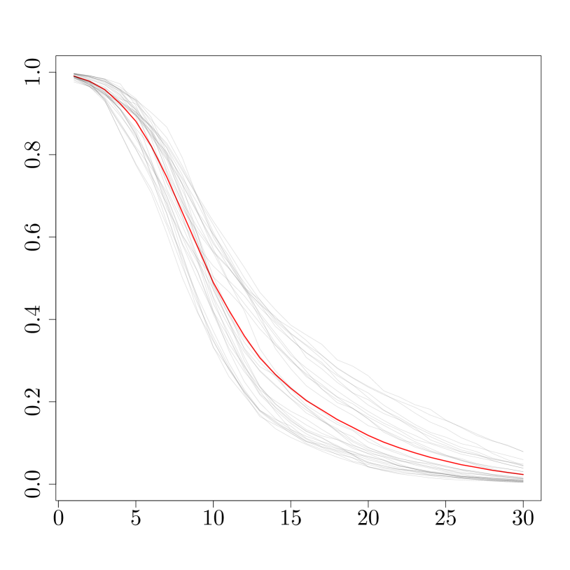
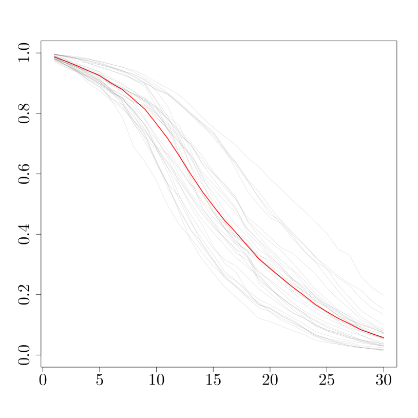
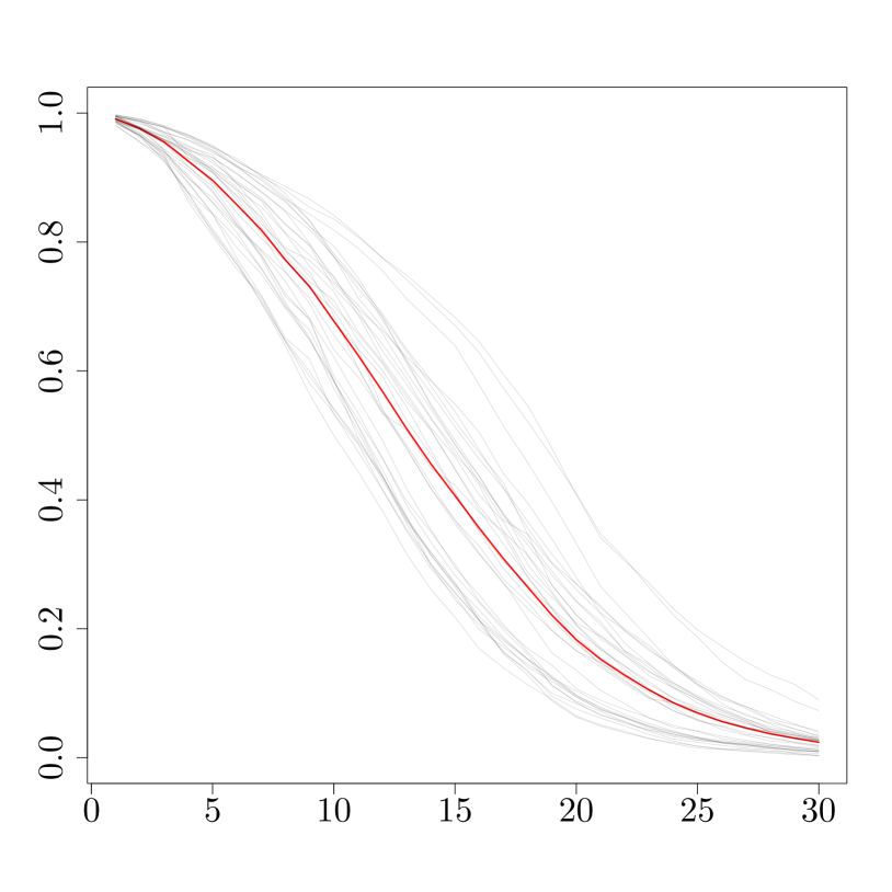
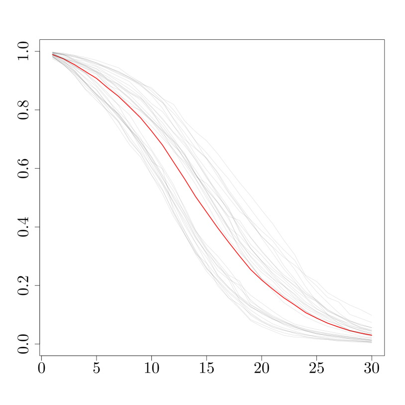
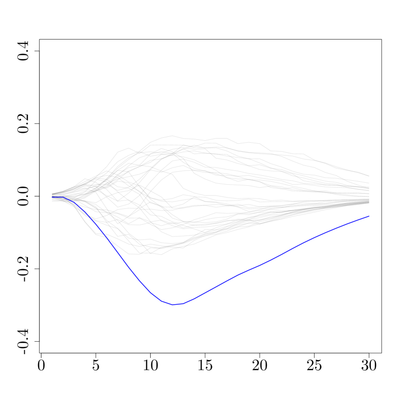
(a)

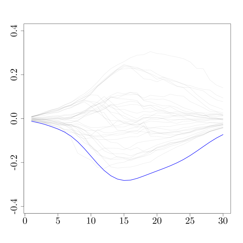
(b)

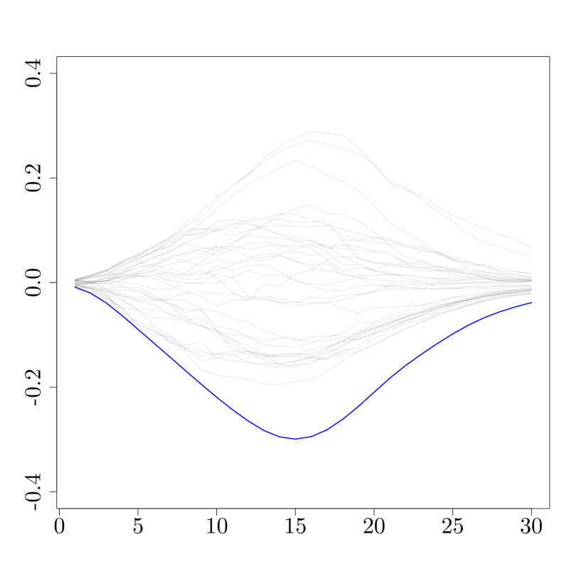
(c)

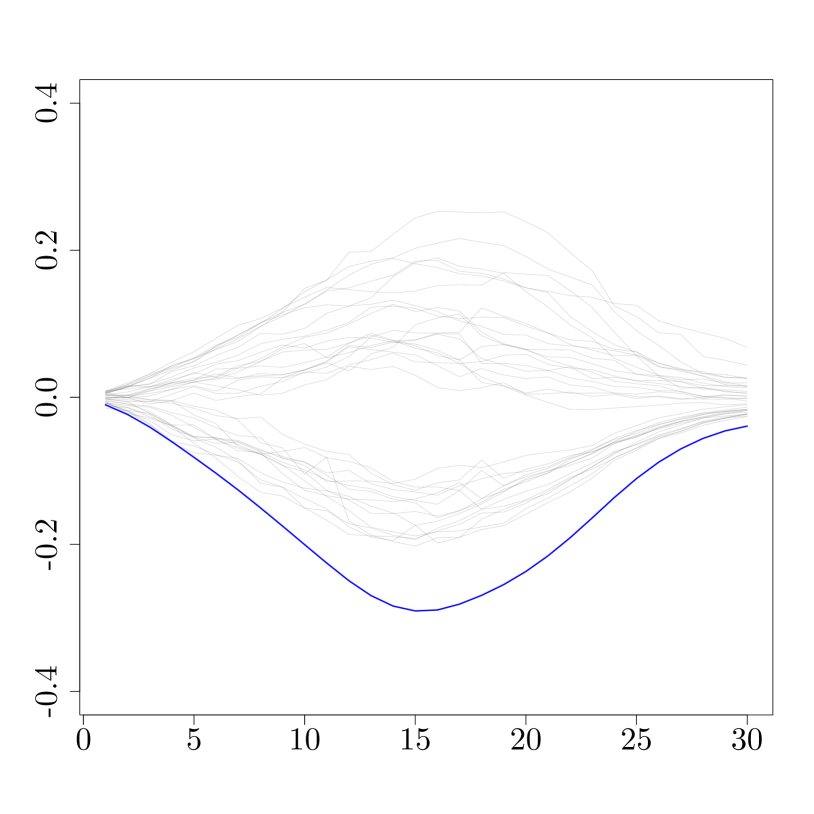
(d)

Figure 1: Survival functions of cohorts of medflies: (a) Females on a sugar diet, (b) Females on a protein plus sugar diet, (c) Males on a sugar diet, and (d) Males on a protein plus sugar diet; (Top row) Gray lines: survival functions of samples, Red line: mean function, (Bottom row) Gray lines: deviation of samples from the mean function, Blue line: first eigenfunction of covariance operators, which accounts for 89.3%, 94.5%, 96.4% and 97.8% of the variation of survival functions in each of four groups respectively.

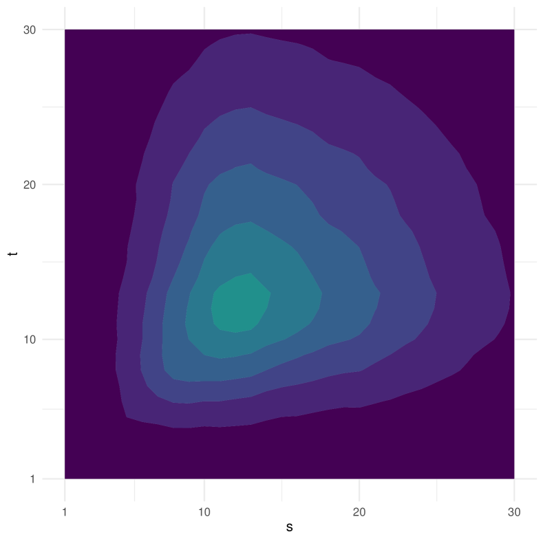
(a)

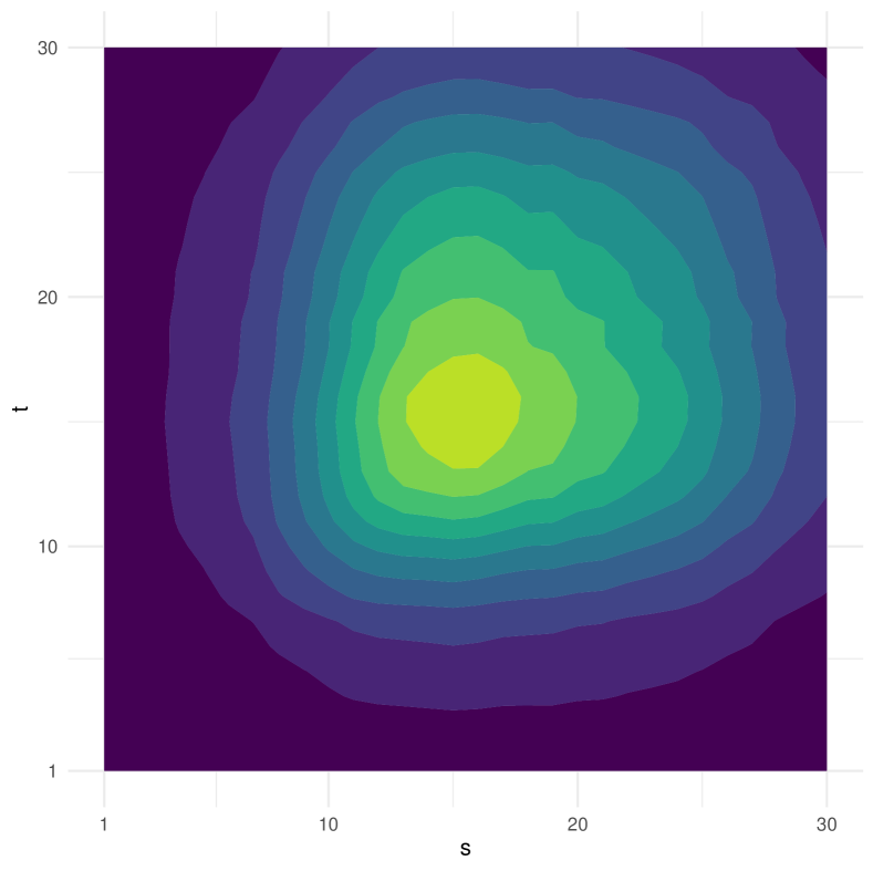
(b)

(c)

(d)

Figure 2: Estimated covariance functions of the four groups of medflies: (a) Females on a sugar diet, (b) Females on a protein plus sugar diet, (c) Males on a sugar diet, and (d) Males on a protein plus sugar diet.

The panels in the first row demonstrate 33 sample functions in each group as well as the mean functions, and each sample function is the survival rate of medflies in one cage. The panels in the second row demonstrate deviation of samples from the group’s mean function as well as the first eigenfunction of the covariance operator. The first eigenfunction explains the major variation of functional samples within each group (89.3%, 94.5%, 96.4%, and 97.8% in each group respectively). It could be noticed that there is a slight difference in eigenvalues and eigenfunctions of covariance operators between groups. The kernel functions of the covariance operators in the four groups are depicted in Figure 2, which magnifies the between-groups difference of covariance operators. MMD and the four other tests including $L^{2}$, $T_{\max}$, GPF and $F_{\max}$ were employed to test the equality of covariance operators. The results are presented in Table 7.

It can be understood that the p-values of all pair-wise comparisons are generally smaller than of the other four tests. As described in Guo et al. [11], it was expected that $F_{\max}$ test to have higher power than $GPF$ in this data set. However, as it is shown in simulation studies, MMD has higher power than both $F_{\max}$ and $GPF$ in all of the scenarios.

Table 7: p-Values (in percent) of $L^{2}$, $T_{\max}$, GPF, $F_{\max}$ and MMD tests
applied to compare covariance operators of survival functions of the four groups of medflies.

	$L^{2}$	$T_{\max}$	GPF	$F_{\max}$	MMD
(a) vs (b)	01.4	00.4	00.6	0.1	0.1
(a) vs (c)	06.2	00.6	03.4	0.1	0.1
(a) vs (d)	00.1	00.1	00.1	0.1	0.1
(b) vs (c)	21.2	29.2	12.2	3.6	0.1
(b) vs (d)	33.8	47.0	13.8	1.2	0.2
(c) vs (d)	24.0	27.8	21.2	6.2	2.6
All Groups	02.6	001.8	00.4	0.1	0.1

5 Conclusions and Discussion

This study explored kernel methods for probability measures and their applications to functional data analysis. We derived conditions of kernels that are characteristic for infinite-dimensional separable Hilbert spaces. We also derived a framework for introducing a pseudo-likelihood function over infinite-dimensional separable Hilbert spaces. It is shown that the MKM estimators for location and covariance operator obtained by maximizing this pseudo-likelihood function coincide with ordinary least square estimators, which is the same as what we observe in finite-dimensional spaces where ordinary least square estimators coincide with MLE in the case of Gaussian distribution. We also used Maximum Mean Discrepancy as a distance over the space of Gaussian probability measures induced by functional response models and derived new powerful tests for the problems of functional one-way ANOVA and homogeneity of covariance operators. An important question which we have not covered in this paper is how to choose the Gaussian kernel bandwidth parameter $\sigma$. As it is also proposed in Sriperumbudur et al. [26], one may choose a family of characteristic kernels $\left\{k_{\sigma}\left(x,y\right):=exp\left(-\sigma\left\|x-y\right\|^{2}\right),~{}\sigma>0\right\}$ and use the maximal RKHS distance $\gamma\left(\mathbb{P},\mathbb{Q}\right)=\sup_{\sigma>0}{\gamma_{\sigma}\left(\mathbb{P},\mathbb{Q}\right)}$ where $\gamma_{\sigma}$ is the MMD metric defined by characteristic kernel $k_{\sigma}$. $\gamma$ is a stronger metric than $\gamma_{\sigma}$, so new tests derived from $\gamma$ must have a better performance than those introduced in section 4.

Appendix A Appendix

A.1 Proof of Theorem 1 and Corollary 2

To provide the proof of Theorem 1 we need the following lemma:

Lemma 11.

Let $\{b_{j}\}$ be a descending sequence of positive real numbers and $\{a_{j}\}$ be a series of real numbers such that $\sum_{j\geq 1}\left|a_{j}\right|<\infty$ and $\sum_{j\geq 1}a_{j}b_{j}>0$. Then there exists a finite $N\in\mathbb{N}$ such that $\sum_{j=1}^{N}a_{j}>0$.

• Let $P=\left\{n_{1},n_{2},\ldots\right\}\subseteq\mathbb{N}$ be the set of indices for which $a_{j}>0$, define $n_{0}=0$ and for any $n_{i}\in P$, let $T_{n_{i}}=\mathbb{N}\cap(n_{i-1},n_{i}]$. Then for any $i\geq 1$, we have $b_{n_{i}}\sum_{j\in T_{n_{i}}}a_{j}\geq\sum_{j\in T_{n_{i}}}b_{j}a_{j}.$ Let $n_{k}\in P$ be the first index such that $\sum\limits_{j=1}^{n_{k}}a_{j}b_{j}>0$. If $k=1$, the proof is straightforward. If $k>1$, then

  $$\sum_{j=1}^{n_{k}}a_{j}=\sum_{i=1}^{k}\sum_{j\in T_{n_{i}}}a_{j} \geq\sum_{i=1}^{k}\frac{1}{b_{n_{i}}}\sum_{j\in T_{n_{i}}}b_{j}a_{j}\geq\frac{1}{b_{n_{k-1}}}\sum_{i=1}^{k-1}\sum_{j\in T_{n_{i}}}b_{j}a_{j}+\frac{1}{b_{n_{k}}}\sum_{j\in T_{n_{i}}}b_{j}a_{j}$$

  $$\geq\frac{1}{b_{n_{k-1}}}\sum_{i=1}^{k}\sum_{j\in T_{n_{i}}}b_{j}a_{j}=\frac{1}{b_{n_{k-1}}}\sum_{j=1}^{n_{k}}b_{j}a_{j}>0.$$

  ∎

Suppose $m_{P_{2}}(y)-m_{P_{1}}(y)=\delta>0$. There exists $r>0$ big enough such that $\sup\limits_{x\in B_{r}(y)^{c}}\psi(\left\|x-y\right\|_{\mathbb{H}})\leq\delta/2$, in which $B_{r}(y)=\{x\in\mathbb{H}\>\text{s.t}\>\left\|x-y\right\|_{\mathbb{H}}<r\}$. Then, we have

$$0<\delta =\int\limits_{\mathbb{H}}\psi(\left\|x-y\right\|_{\mathbb{H}})(P_{2}-P_{1})(dx)$$

$$=\int\limits_{B_{r}(y)}\psi(\left\|x-y\right\|_{\mathbb{H}})(P_{2}-P_{1})(dx)+\int\limits_{B_{r}(y)^{c}}\psi(\left\|x-y\right\|_{\mathbb{H}})(P_{2}-P_{1})(dx)$$

$$\leq\int\limits_{B_{r}(y)}\psi(\left\|x-y\right\|_{\mathbb{H}})(P_{2}-P_{1})(dx)+\delta/2$$

and thus

$$\int\limits_{B_{r}(y)}\psi(\left\|x-y\right\|_{\mathbb{H}})(P_{2}-P_{1})(dx)\geq\frac{\delta}{2}>0.$$ (18)

Let define

• $r_{i,L}=(1-L^{i})r$ ; $i\geq 1$ , $L\in(0,1)$

• $B_{i,L}=B_{r_{i,L}}(y)$ ; $i\geq 1$

• $B_{1,L}^{{}^{\prime}}=B_{1,L}$ , $B_{i,L}^{{}^{\prime}}=B_{i,L}\backslash B_{\left(i-1\right),L}$ ; $i\geq 2$

thus from (18) we have

$$0<\frac{\delta}{2} \leq\sum_{i\geq 1}\int\limits_{B_{i,L}^{{}^{\prime}}}\psi(\left\|x-y\right\|_{\mathbb{H}})(P_{2}-P_{1})(dx)$$

$$\leq\sum_{i\geq 1}m_{i,L}(P_{2}-P_{1})(B_{i,L}^{{}^{\prime}})+\sum_{i\geq 1}\gamma_{i,L}P_{2}(B_{i,L}^{{}^{\prime}})$$

$$\leq\sum_{i\geq 1}m_{i,L}(P_{2}-P_{1})(B_{i,L}^{{}^{\prime}})+\sup_{i\geq 1}\gamma_{i,L}P_{2}\left(B_{r}(y)\right),$$

where $m_{i,L}=\inf\limits_{x\in B_{i,L}^{{}^{\prime}}}\psi(\left\|x-y\right\|_{\mathbb{H}})$ and $M_{i,L}=\sup\limits_{x\in B_{i,L}^{{}^{\prime}}}\psi(\left\|x-y\right\|_{\mathbb{H}})$ and $\gamma_{i,L}=M_{i,L}-m_{i,L}$. Because $\psi$ is a bounded non-negative continuous and strictly decreasing function, we can choose $L\in\left(0,1\right)$ such that $\sup_{i\geq 1}\gamma_{i,L}P_{2}\left(B_{r}(y)\right)<\frac{\delta}{4}$ or $\sup_{i\geq 1}\gamma_{i,L}<\frac{\delta}{4P_{2}\left(B_{r}(y)\right)}$ and thus $\sum_{i\geq 1}m_{i,L}(P_{2}-P_{1})(B_{i,L}^{{}^{\prime}})>0$. By lemma 11 there exists $N<\infty$ such that $\sum_{i=1}^{N}\left(P_{2}-P_{1}\right)\left(B_{i,L}^{{}^{\prime}}\right)>0$, which immediately follows that $\left(P_{2}-P_{1}\right)\left(B_{r^{*}}(y)\right)>0$, where $r^{*}=\left(1-L^{N}\right)r$. ∎

Let assume $\int_{\mathbb{H}}\psi(\left\|x-y_{2}\right\|_{\mathbb{H}})P(dx)>\int_{\mathbb{H}}\psi(\left\|x-y_{1}\right\|_{\mathbb{H}})P(dx)$ and let $P_{-a}$ be the push forward of $P$ by the map $x\mapsto x+a$, which translates $x$ to $x+a$, then we have $\int_{\mathbb{H}}\psi(\left\|x\right\|_{\mathbb{H}})P_{-y_{2}}(dx)>\int_{\mathbb{H}}\psi(\left\|x\right\|_{\mathbb{H}})P_{-y_{1}}(dx)$ and thus by the same argument as stated in the proof of Theorem 1 there exists $r>0$ big enough such that $\left(P_{-y_{2}}-P_{-y_{1}}\right)\left(B_{r}\left(0\right)\right)>0$ and consequently $P\left(B_{r}(y_{2})\right)>P\left(B_{r}(y_{1})\right)$. ∎

A.2 Proof of Theorem 4

The existence proof of a continuous characteristic kernel for $\ell_{2}$ relies on the following theorem by Steinwart and Ziegel [28]. We also need lemma 13 to complete the proof.

Theorem 12.

[28, Theorem 3.14] For a compact topological Hausdorff space $\left(X,\tau\right)$, the following statements are equivalent:

1. There exists a universal kernel $k$ on $X$.

2. There exists a continuous characteristic kernel $k$ on $X$.

3. $X$ is metrizable, i.e. there exists a metric generating the topology $\tau$.

Lemma 13.

Let $\overline{\mathbb{R}}$ be the extended real line, and $\overline{\mathbb{R}}^{\infty}$ and $\mathbb{R}^{\infty}$ be the countable products of $\overline{\mathbb{R}}$ and $\mathbb{R}$ respectively, which are equipped with the product topologies, and let $\ell_{2}\subset\overline{\mathbb{R}}^{\infty}$ be the Hilbert space of square summable sequences. If the function $f:\overline{\mathbb{R}}^{\infty}\to\mathbb{R}$ is continuous, then $f|_{\ell^{2}}$, which is restriction of $f$ to $\ell_{2}$, is continuous with respect to the norm of $\ell_{2}$.

• Assume that $\varphi:\overline{\mathbb{R}}\to[-1,1]$ is defined as follows:

  $$\varphi(x)=\frac{x}{1+|x|},~{}~{}~{}~{}\forall x\in\mathbb{R}~{}~{}\mbox{and}~{}~{}~{}\varphi(-\infty)=-1,~{}~{}~{}\varphi(+\infty)=1.$$

  It is clear that $\varphi$ is a homeomorphic and order-preserving. Consider

  $$\rho(x,y):=|\varphi(x)-\varphi(y)|,~{}~{}~{}\mbox{for~{}all}~{}x,y\in\overline{\mathbb{R}}.$$

  Then $\rho$ is a metric and the topology induced by this metric is equivalent to the order topology. On the other hand, it is well known that the product topology on $\overline{\mathbb{R}}^{\infty}$ can be generated by the following metric [4, Theorem 2.6.6],

  $$d(x,y):=\sum_{k=1}^{\infty}\frac{\rho(x_{k},y_{k})}{2^{k}\left(1+\rho(x_{k},y_{k})\right)},\quad\forall x=(x_{k}),y=(y_{k})\in\overline{\mathbb{R}}^{\infty}.$$

  Now, we show that the topology induced by the metric $d$ on $\ell^{2}$ is weaker than the norm topology. For this purpose, let $x_{n}=(x_{n}^{k}),x=(x^{k})\in\ell^{2}$ and $\|x_{n}-x\|\to 0$. Therefore, $|x_{n}^{k}-x^{k}|\to 0$ for all $k\in\mathbb{N}$. Because $\varphi$ is a homeomorphic, $\rho(x_{n}^{k},x^{k})\to 0$ for any $k\in\mathbb{N}$ and hence $d(x_{n},x)\to 0$. Thus, if $f$ is continuous with respect to the product topology, then $f|_{\ell^{2}}$ is continuous with respect to the norm topology. ∎

Without loss of generality assume $\mathbb{H}$ to be the space of square summable sequences $\ell_{2}$, which is a subset of $\mathbb{R}^{\infty}$, and let $\mathcal{B}\left(\ell_{2}\right)$ be Borel sigma-algebra generated by the open sets of $\ell_{2}$. $\mathbb{R}$ is a one-dimensional locally compact Hausdorff space, and the extended real line $\overline{\mathbb{R}}$ equipped with order topology is a metrizable Hausdorff and compact topological space. Equip both $\mathbb{R}^{\infty}$ and $\overline{\mathbb{R}}^{\infty}$ with the product topologies and let $\mathcal{B}\left(\mathbb{R}^{\infty}\right)$ and $\mathcal{B}\left(\overline{\mathbb{R}}^{\infty}\right)$ be the Borel sigma-algebra generated by the open sets of these topologies. Consider that $\mathcal{B}\left(\ell_{2}\right)=\left\{A\cap\ell_{2}:A\in\mathcal{B}\left(\mathbb{R}^{\infty}\right)\right\}$, and we have $\mathcal{B}\left(\ell_{2}\right)\subseteq\mathcal{B}\left(\mathbb{R}^{\infty}\right)\subseteq\mathcal{B}\left(\overline{\mathbb{R}}^{\infty}\right)$. Note that $\mathcal{B}\left(\mathbb{R}^{\infty}\right)\subseteq\mathcal{B}\left(\overline{\mathbb{R}}^{\infty}\right)$ Because we equipped extended real line $\overline{\mathbb{R}}$ with order topology, which includes the bases for the natural topology of $\mathbb{R}$. Let $\iota:\ell_{2}\to\overline{\mathbb{R}}^{\infty}$ be the usual inclusion map, then for every $A\in\mathcal{B}\left(\overline{\mathbb{R}}^{\infty}\right)$ we have $\iota^{-1}\left(A\right)=A\cap\ell_{2}\in\mathcal{B}\left(\ell_{2}\right)$, so $\iota$ is a $\mathcal{B}\left(\ell_{2}\right)-\mathcal{B}\left(\overline{\mathbb{R}}^{\infty}\right)$ measurable map and hence every $\ell_{2}$-valued random element is an $\overline{\mathbb{R}}^{\infty}$-valued random element and thus the space of Borel probability measures on $\left(\ell_{2},\mathcal{B}\left(\ell_{2}\right)\right)$ is a subset of the space of Borel probability measures on $\left(\overline{\mathbb{R}}^{\infty},\mathcal{B}\left(\overline{\mathbb{R}}^{\infty}\right)\right)$. $\overline{\mathbb{R}}^{\infty}$ itself is a metrizable compact topological Hausdorff space, thus by invoking Lemma 12, there exists a continuous characteristic kernel $k\left(\cdot,\cdot\right)$ on $\overline{\mathbb{R}}^{\infty}$, which by employing Lemma 13, its restriction to $\ell_{2}$ is also continuous with respect to the norm of $\ell_{2}$. ∎

A.3 Proof of Theorem 5

Let $\ell_{2}$ be the space of square summable sequences with inner product $\left\langle\cdot,\cdot\right\rangle$ and norm $\left\|\cdot\right\|$, and let $\Lambda_{\theta}$ be the infinite-dimensional Gaussian measure on the measurable space $\left(\mathbb{R}^{\infty},\mathcal{B}\left(\mathbb{R}^{\infty}\right)\right)$ defined as the product of countably many copies of normal distribution with mean zero and variance $\theta$. The dual space of $\mathbb{R}^{\infty}$ is $c_{00}$, so characteristic function of Gaussian measure, for any $x\in c_{00}$ equals to

$$\psi\left(x\right):=\int\limits_{\mathbb{R}^{\infty}}e^{-i\left\langle\omega,x\right\rangle}\Lambda_{2\sigma}\left(d\omega\right)=e^{-\sigma\left\|x\right\|^{2}}.$$ (19)

Let $\mathbb{P}$ and $\mathbb{Q}$ be two arbitrary probability measures over $c_{00}$ such that $\gamma_{k}\left(\mathbb{P},\mathbb{Q}\right)=0$, then

$$0=\gamma_{k}\left(\mathbb{P},\mathbb{Q}\right)^{2} =\int\limits_{c_{00}}\int\limits_{c_{00}}e^{-\sigma\left\|x-y\right\|^{2}}\left(\mathbb{P}-\mathbb{Q}\right)\left(dx\right)\left(\mathbb{P}-\mathbb{Q}\right)\left(dy\right)$$

$$=\int\limits_{c_{00}}\int\limits_{c_{00}}\left(\int\limits_{\mathbb{R}^{\infty}}e^{-i\left\langle\omega,x-y\right\rangle}\Lambda_{2\sigma}\left(d\omega\right)\right)\left(\mathbb{P}-\mathbb{Q}\right)\left(dx\right)\left(\mathbb{P}-\mathbb{Q}\right)\left(dy\right)$$

$$\stackrel{{\scriptstyle(a)}}{{=}}\int\limits_{\mathbb{R}^{\infty}}\left(\int\limits_{c_{00}}\int\limits_{c_{00}}e^{-i\left\langle\omega,x-y\right\rangle}\left(\mathbb{P}-\mathbb{Q}\right)\left(dx\right)\left(\mathbb{P}-\mathbb{Q}\right)\left(dy\right)\right)\Lambda_{2\sigma}\left(d\omega\right)$$

$$=\int\limits_{\mathbb{R}^{\infty}}\left(\int\limits_{c_{00}}e^{-i\left\langle\omega,x\right\rangle}\left(\mathbb{P}-\mathbb{Q}\right)\left(dx\right)\int\limits_{c_{00}}e^{i\left\langle\omega,y\right\rangle}\left(\mathbb{P}-\mathbb{Q}\right)\left(dy\right)\right)\Lambda_{2\sigma}\left(d\omega\right)$$

$$=\int\limits_{\mathbb{R}^{\infty}}\left(\phi_{\mathbb{P}}\left(\omega\right)-\phi_{\mathbb{Q}}\left(\omega\right)\right)\left(\overline{\phi_{\mathbb{P}}\left(\omega\right)}-\overline{\phi_{\mathbb{Q}}\left(\omega\right)}\right)\Lambda_{2\sigma}\left(d\omega\right)$$

$$=\int\limits_{\mathbb{R}^{\infty}}\left|\phi_{\mathbb{P}}\left(\omega\right)-\phi_{\mathbb{Q}}\left(\omega\right)\right|^{2}\Lambda_{2\sigma}\left(d\omega\right).$$ (20)

In the above equation, Fubini-Tonneli’s theorem is invoked in (a). Dual of $c_{00}$ with norm $\left\|\cdot\right\|$, is the space of square summable sequences $\ell_{2}$. So to show that $\mathbb{P}=\mathbb{Q}$, it is enough to show that $\phi_{\mathbb{P}}=\phi_{\mathbb{Q}}$ agrees on $\ell_{2}$. By (20) and by definition of the integral and the fact that $\text{supp}\left(\Lambda_{2\sigma}\right)=\mathbb{R}^{\infty}$, for any open set $B$ we have,

$$\inf_{\omega\in B}\left|\phi_{\mathbb{P}}\left(\omega\right)-\phi_{\mathbb{Q}}\left(\omega\right)\right|^{2}=0.$$

Fix $\omega_{0}\in c_{00}$, and for any $m\in\mathbb{N}$ define

$$B_{m}:=\left\{x\in\mathbb{R}^{m}:\sum_{i=1}^{m}\left(x_{i}-\omega_{0i}\right)^{2}<\frac{1}{m^{2}}\right\}\times\mathbb{R}^{\infty},$$

which is an open set in $\mathbb{R}^{\infty}$. Thus for each $m\in\mathbb{N}$, we have,

$$\inf_{\omega\in B_{m}}\left|\phi_{\mathbb{P}}\left(\omega\right)-\phi_{\mathbb{Q}}\left(\omega\right)\right|^{2}=0,$$

and so there exists $\omega_{m}\in B_{m}$ such that, $\left|\phi_{\mathbb{P}}\left(\omega_{m}\right)-\phi_{\mathbb{Q}}\left(\omega_{m}\right)\right|^{2}<\frac{1}{m}.$ Confirm that the sequence $\omega_{m}$ converges in the metric of $\mathbb{R}^{\infty}$ to $\omega_{0}$, since

$$d\left(\omega_{m},\omega_{0}\right) =\sum_{k\geq 1}2^{-k}\frac{\left|\omega_{mk}-\omega_{0k}\right|}{1+\left|\omega_{mk}-\omega_{0k}\right|}\leq\sum_{k=1}^{m}2^{-k}\frac{\nicefrac{{1}}{{m}}}{1+\nicefrac{{1}}{{m}}}+\sum_{k>m}2^{-k}$$

$$\leq\frac{1}{m+1}\left(1-2^{-m}\right)+2^{-m}\to 0.$$

So $\left\langle\omega_{m},x\right\rangle\to\left\langle\omega_{0},x\right\rangle$ for any $x\in c_{00}$. By a simple application of Bounded Convergence Theorem, we have

$$\lim_{m\to\infty}\left|\phi_{\mathbb{P}}\left(\omega_{m}\right)-\phi_{\mathbb{Q}}\left(\omega_{m}\right)\right|^{2} =\lim_{m\to\infty}\left|\int\limits_{c_{00}}e^{-i\left\langle\omega_{m},x\right\rangle}\mathbb{P}\left(dx\right)-\int\limits_{c_{00}}e^{-i\left\langle\omega_{m},x\right\rangle}\mathbb{Q}\left(dx\right)\right|^{2}$$

$$=\left|\int\limits_{c_{00}}\lim_{m\to\infty}e^{-i\left\langle\omega_{m},x\right\rangle}\mathbb{P}\left(dx\right)-\int\limits_{c_{00}}\lim_{m\to\infty}e^{-i\left\langle\omega_{m},x\right\rangle}\mathbb{Q}\left(dx\right)\right|^{2}$$

$$=\left|\int\limits_{c_{00}}e^{-i\left\langle\omega_{0},x\right\rangle}\mathbb{P}\left(dx\right)-\int\limits_{c_{00}}e^{-i\left\langle\omega_{0},x\right\rangle}\mathbb{Q}\left(dx\right)\right|^{2}$$

$$=\left|\phi_{\mathbb{P}}\left(\omega_{0}\right)-\phi_{\mathbb{Q}}\left(\omega_{0}\right)\right|^{2}$$

and thus

$$\left|\phi_{\mathbb{P}}\left(\omega_{0}\right)-\phi_{\mathbb{Q}}\left(\omega_{0}\right)\right|^{2}=\lim_{m\to\infty}\left|\phi_{\mathbb{P}}\left(\omega_{m}\right)-\phi_{\mathbb{Q}}\left(\omega_{m}\right)\right|^{2}\leq\lim_{m\to\infty}\frac{1}{m}\to 0.$$

So $\phi_{\mathbb{P}}=\phi_{\mathbb{Q}}$ on $c_{00}$. The space $c_{00}$ is dense in $\ell_{2}$, so $\phi_{\mathbb{P}}=\phi_{\mathbb{Q}}$ agrees on $\ell_{2}$ and thus $\mathbb{P}=\mathbb{Q}$.

A.4 Proof of Proposition 6

Before providing the proof we need some tools, which are provided in the upcoming theorems and lemmas. The next theorem is a generalization of Ky Fan’s inequality, which is useful to show convexity of the map $A\mapsto\left|I+A\right|^{-\nicefrac{{1}}{{2}}}$ on the convex set of positive trace-class operators that is crucial to prove Gaussian kernel is characteristic for the family of Gaussian distributions. The following theorem is a special case of Minh [19, Theorem 1] when $\mu=\gamma=1$.

Theorem 14.

Let $\mathbb{H}$ be an infinite-dimensional separable Hilbert space, and $A$, $B$ two arbitrary positive trace-class operators, for $0\leq\alpha\leq 1$

$$\left|\alpha\left(I+A\right)+\left(1-\alpha\right)\left(I+B\right)\right|\geq\left|I+A\right|^{\alpha}\left|I+B\right|^{1-\alpha}.$$

For $0<\alpha<1$, equality occurs if and only if $A=B$.

Lemma 15.

Let $\mathbb{H}$ be a separable Hilbert space, and let $\left|\cdot\right|$ be the determinant of a non-negative symmetric operator on $\mathbb{H}$. $A\mapsto\left|I+A\right|^{-\nicefrac{{1}}{{2}}}$ is a convex function over the convex set of positive trace-class operators on $\mathbb{H}$, and for any two arbitrary positive trace-class operators $A$ and $B$,

$$2\left|I+\frac{A+B}{2}\right|^{-\nicefrac{{1}}{{2}}}\leq\left|I+A\right|^{-\nicefrac{{1}}{{2}}}+\left|I+B\right|^{-\nicefrac{{1}}{{2}}}$$

and $2\left|I+\frac{A+B}{2}\right|^{-\nicefrac{{1}}{{2}}}=\left|I+A\right|^{-\nicefrac{{1}}{{2}}}+\left|I+B\right|^{-\nicefrac{{1}}{{2}}}$ if and only if $A=B$.

• By Theorem 14 we have

  $$\log\left|I+\left(\alpha A+\left(1-\alpha\right)B\right)\right|\geq\alpha\log\left|I+A\right|+\left(1-\alpha\right)\log\left|I+B\right|,$$

  so $A\mapsto\log\left|I+A\right|$ is a concave function on the convex set of positive trace-class operators, and thus $A\mapsto\log\left|I+A\right|^{\nicefrac{{-1}}{{2}}}$ is a convex function and also is $A\mapsto\left|I+A\right|^{\nicefrac{{-1}}{{2}}}$, since $x\mapsto e^{x}$ is a non-decreasing convex function. Consequently

  $$\left|I+\left(\frac{1}{2}A+\frac{1}{2}B\right)\right|^{\nicefrac{{-1}}{{2}}}\leq\frac{1}{2}\left|I+A\right|^{-\nicefrac{{1}}{{2}}}+\frac{1}{2}\left|I+B\right|^{-\nicefrac{{1}}{{2}}}$$

  and thus

  $$2\left|I+\frac{A+B}{2}\right|^{-\nicefrac{{1}}{{2}}}\leq\left|I+A\right|^{-\nicefrac{{1}}{{2}}}+\left|I+B\right|^{-\nicefrac{{1}}{{2}}}.$$

  By invoking Theorem (14), equality occurs if and only if $A=B$. ∎

Lemma 16.

[18, Proposition 1.2.8] Let $\mathbb{H}$ be a separable Hilbert space and $\mathcal{N}\left(\mu,C\right)$ be a Gaussian probability measure on $\mathbb{H}$ with mean function $\mu$ and covariance operator $C$. For any $\sigma>0$

$$\int\limits_{\mathbb{H}}e^{-\sigma\left\|x\right\|_{\mathbb{H}}^{2}}\mathcal{N}\left(\mu,C\right)\left(dx\right)=\left|I+2\sigma C\right|^{-\nicefrac{{1}}{{2}}}e^{-\sigma\left\langle\left(I+2\sigma C\right)^{-1}\mu,\mu\right\rangle}.$$

If $Y\sim\mathcal{N}\left(\mu,\boldsymbol{C}\right)$ then by lemma 16 we have

$$m_{P}(x) =\int\limits_{\mathbb{H}}e^{-\sigma\left\|y-x\right\|_{\mathbb{H}}^{2}}\mathcal{N}\left(\mu,\boldsymbol{C}\right)\left(dy\right)=\int\limits_{\mathbb{H}}e^{-\sigma\left\|z\right\|_{\mathbb{H}}^{2}}\mathcal{N}\left(x-\mu,\boldsymbol{C}\right)\left(dz\right)$$

$$=\left|I+2\sigma\boldsymbol{C}\right|^{-1/2}e^{-\sigma\left\langle\left(I+2\sigma\boldsymbol{C}\right)^{-1}\left(x-\mu\right),\left(x-\mu\right)\right\rangle}.$$

Let $T_{1}=I+2\sigma C_{1}$, then

$$\left\langle m_{P_{1}},m_{P_{2}}\right\rangle_{\mathcal{H}_{k}} =\int\limits_{\mathbb{H}}\int\limits_{\mathbb{H}}e^{-\sigma\left\|x-y\right\|_{\mathbb{H}}^{2}}\mathcal{N}\left(\mu_{1},C_{1}\right)\left(dx\right)\mathcal{N}\left(\mu_{2},C_{2}\right)\left(dy\right)$$

$$=\int\limits_{\mathbb{H}}\left|T_{1}\right|^{-\nicefrac{{1}}{{2}}}e^{-\sigma\left\langle T_{1}^{-1}\left(y-\mu_{1}\right),\left(y-\mu_{1}\right)\right\rangle}\mathcal{N}\left(\mu_{2},C_{2}\right)\left(dy\right)$$

$$=\left|T_{1}\right|^{-\nicefrac{{1}}{{2}}}\int\limits_{\mathbb{H}}e^{-\sigma\left\langle T_{1}^{\nicefrac{{-1}}{{2}}}\left(y-\mu_{1}\right),T_{1}^{\nicefrac{{-1}}{{2}}}\left(y-\mu_{1}\right)\right\rangle}\mathcal{N}\left(\mu_{2},C_{2}\right)\left(dy\right)$$

$$=\left|T_{1}\right|^{-\nicefrac{{1}}{{2}}}\int\limits_{\mathbb{H}}e^{-\sigma\left\|z\right\|_{\mathbb{H}}^{2}}\mathcal{N}\left(T_{1}^{\nicefrac{{-1}}{{2}}}\left(\mu_{2}-\mu_{1}\right),T_{1}^{\nicefrac{{-1}}{{2}}}C_{2}T_{1}^{\nicefrac{{-1}}{{2}}}\right)\left(dz\right)$$

$$=\left|T_{1}\right|^{-\nicefrac{{1}}{{2}}}\left|I+2\sigma T_{1}^{\nicefrac{{-1}}{{2}}}C_{2}T_{1}^{\nicefrac{{-1}}{{2}}}\right|^{\nicefrac{{-1}}{{2}}}$$

$$\qquad\qquad\qquad e^{-\sigma\left\langle\left(I+2\sigma T_{1}^{\nicefrac{{-1}}{{2}}}C_{2}T_{1}^{\nicefrac{{-1}}{{2}}}\right)^{-1}T_{1}^{\nicefrac{{-1}}{{2}}}\left(\mu_{2}-\mu_{1}\right),T_{1}^{\nicefrac{{-1}}{{2}}}\left(\mu_{2}-\mu_{1}\right)\right\rangle}$$

$$=\left|T_{1}\right|^{-\nicefrac{{1}}{{2}}}\left|I+2\sigma T_{1}^{-1}C_{2}\right|^{\nicefrac{{-1}}{{2}}}$$

$$\qquad\qquad\qquad e^{-\sigma\left\langle T_{1}^{\nicefrac{{-1}}{{2}}}\left(I+2\sigma T_{1}^{\nicefrac{{-1}}{{2}}}C_{2}T_{1}^{\nicefrac{{-1}}{{2}}}\right)^{-1}T_{1}^{\nicefrac{{-1}}{{2}}}\left(\mu_{2}-\mu_{1}\right),\left(\mu_{2}-\mu_{1}\right)\right\rangle}$$

$$=\left|I+2\sigma\left(C_{1}+C_{2}\right)\right|^{\nicefrac{{-1}}{{2}}}e^{-\sigma\left\langle\left(I+2\sigma\left(C_{1}+C_{2}\right)\right)^{-1}\left(\mu_{2}-\mu_{1}\right),\left(\mu_{2}-\mu_{1}\right)\right\rangle},$$

and thus

$$\left\|m_{P_{1}}-m_{P_{2}}\right\|_{\mathcal{H}_{k}}^{2} =\left\|m_{P_{1}}\right\|_{\mathcal{H}_{k}}^{2}+\left\|m_{P_{2}}\right\|_{\mathcal{H}_{k}}^{2}-2\left\langle m_{P_{1}},m_{P_{2}}\right\rangle_{\mathcal{H}_{k}}$$

$$=\left|I+4\sigma C_{1}\right|^{-\nicefrac{{1}}{{2}}}+\left|I+4\sigma C_{2}\right|^{-\nicefrac{{1}}{{2}}}$$

$$\phantom{=}-2\left|I+2\sigma\left(C_{1}+C_{2}\right)\right|^{\nicefrac{{-1}}{{2}}}e^{-\sigma\left\langle\left(I+2\sigma\left(C_{1}+C_{2}\right)\right)^{-1}\left(\mu_{2}-\mu_{1}\right),\left(\mu_{2}-\mu_{1}\right)\right\rangle}.$$

By invoking lemma 15 we have

$$\left|I+4\sigma C_{1}\right|^{-\nicefrac{{1}}{{2}}}+\left|I+4\sigma C_{2}\right|^{-\nicefrac{{1}}{{2}}}\geq 2\left|I+2\sigma\left(C_{1}+C_{2}\right)\right|^{\nicefrac{{-1}}{{2}}},$$

and the equality occurs if and only if $C_{1}=C_{2}$. So $\left\|m_{P_{1}}-m_{P_{2}}\right\|_{\mathcal{H}_{k}}^{2}=0$ if and only if $\mu_{1}=\mu_{2}$ and $C_{1}=C_{2}$. Hence, Gaussian kernel is characteristic for the family of Gaussian distributions. ∎

A.5 Proof of Proposition 7

• We first give a proof for the product-kernel. A proof for the sum-kernel follows the same approach. Let $\mathscr{P}$ be the collection of probability measures on a separable Hilbert space $\mathbb{H}$, and $k\left(\cdot,\cdot\right):\mathbb{H}\times\mathbb{H}\longrightarrow\mathbb{R}$ a characteristic kernel on $\mathbb{H}$. Consider the kernel mean with product-kernel

  $$m_{k^{n}}:\mathscr{P}^{n}\rightarrow\mathbb{\mathcal{H}}_{k^{n}}\qquad\otimes_{j=1}^{n}P_{j}\mapsto m_{\otimes_{i=1}^{n}P_{j}}(x_{1},\ldots,x_{n})$$

  such that for any $x_{1},\ldots,x_{n}\in\mathbb{H}$,

  $$m_{\otimes_{j=1}^{n}P_{j}}(x_{1},\ldots,x_{n}): =\int\limits_{\mathbb{H}^{n}}\left(\prod_{i=1}^{n}k(x_{i},y_{i})\right)\otimes_{j=1}^{n}P_{j}(dy_{j})$$

  $$=\prod_{i=1}^{n}\int\limits_{\mathbb{H}}k(x_{i},y_{i})P_{i}(dy_{i})=\prod_{i=1}^{n}m_{P_{i}}\left(x_{i}\right).$$

  Let $\mathbb{P},\mathbb{Q}\in\mathscr{P}^{n}$ i.e. $\mathbb{P}=\otimes_{j=1}^{n}P_{j}$ , $\mathbb{Q}=\otimes_{j=1}^{n}Q_{j}$ such that $\mathbb{P}\neq\mathbb{Q}$. Given $k$ is characteristic on $\mathbb{H}$, there exists $1\leq i\leq n$ such that $P_{i}\neq Q_{i}$ and $m_{P_{i}}\left(\cdot\right)\neq m_{Q_{i}}\left(\cdot\right)$, thus there exists $\left(x_{n}\right)\in\mathbb{H}^{n}$ such that $\prod_{i=1}^{n}m_{P_{i}}\left(x_{i}\right)\neq\prod_{i=1}^{n}m_{Q_{i}}\left(x_{i}\right)$. Similarly let

  $$m_{k^{n}}:\mathscr{P}^{n}\rightarrow\mathbb{\mathcal{H}}_{k^{n}}\qquad\otimes_{j=1}^{n}P_{j}\mapsto m_{\otimes_{i=1}^{n}P_{j}}(x_{1},\ldots,x_{n})$$

  such that for any $x_{1},\ldots,x_{n}\in\mathbb{H}$,

  $$m_{\otimes_{i=1}^{n}P_{j}}(x_{1},\ldots,x_{n}): =\int\limits_{\mathbb{H}^{n}}\left(\sum_{i=1}^{n}k(x_{i},y_{i})\right)\otimes_{j=1}^{n}P_{j}(dy_{j})$$

  $$=\sum_{i=1}^{n}\int\limits_{\mathbb{H}}k(x_{i},y_{i})P_{i}(dy_{i})=\sum_{i=1}^{n}m_{P_{i}}\left(x_{i}\right).$$

  Let $\mathbb{P},\mathbb{Q}\in\mathscr{P}^{n}$ i.e. $\mathbb{P}=\otimes_{j=1}^{n}P_{j}$ , $\mathbb{Q}=\otimes_{j=1}^{n}Q_{j}$ and $\mathbb{P}\neq\mathbb{Q}$. Given $k$ is characteristic on $\mathbb{H}$, there exists $1\leq i\leq n$ such that $P_{i}\neq Q_{i}$ and $m_{P_{i}}\left(\cdot\right)\neq m_{Q_{i}}\left(\cdot\right)$, thus there exists $\left(x_{n}\right)\in\mathbb{H}^{n}$ such that $\sum_{i=1}^{n}m_{P_{i}}\left(x_{i}\right)\neq\sum_{i=1}^{n}m_{Q_{i}}\left(x_{i}\right)$. ∎

References

• Carey et al. [1992] J.R. Carey, P. Liedo, D. Orozco, and J.W. Vaupel. Slowing of mortality rates at older ages in large medfly cohorts. Science, 258(5081):457–461, 1992. ISSN 0036-8075. doi: 10.1126/science.1411540. URL https://science.sciencemag.org/content/258/5081/457. cited By 419.
• Chiou et al. [2003] Jeng-Min Chiou, Hans-Georg Müller, Jane-Ling Wang, and James R. Carey. A functional multiplicative effects model for longitudinal data, with application to reproductive histories of female medflies. Statist. Sinica, 13(4):1119–1133, 2003. ISSN 1017-0405.
• Choi and Reimherr [2018] Hyunphil Choi and Matthew Reimherr. A geometric approach to confidence regions and bands for functional parameters. J. R. Stat. Soc. Ser. B. Stat. Methodol., 80(1):239–260, 2018. ISSN 1369-7412. doi: 10.1111/rssb.12239.
• Conway [2014] John B. Conway. A course in point set topology. Undergraduate Texts in Mathematics. Springer, Cham, 2014. ISBN 978-3-319-02367-0; 978-3-319-02368-7. doi: 10.1007/978-3-319-02368-7. URL https://doi-org.wcmq.idm.oclc.org/10.1007/978-3-319-02368-7.
• Delaigle and Hall [2010] Aurore Delaigle and Peter Hall. Defining probability density for a distribution of random functions. Ann. Statist., 38(2):1171–1193, 2010. ISSN 0090-5364. doi: 10.1214/09-AOS741.
• Gill et al. [2014] Tepper Gill, Aleks Kirtadze, Gogi Pantsulaia, and Anatolij Plichko. Existence and uniqueness of translation invariant measures in separable Banach spaces. Funct. Approx. Comment. Math., 50(2):401–419, 2014. ISSN 0208-6573. doi: 10.7169/facm/2014.50.2.12. URL https://doi-org.wcmq.idm.oclc.org/10.7169/facm/2014.50.2.12.
• Gneiting and Raftery [2007] Tilmann Gneiting and Adrian E. Raftery. Strictly proper scoring rules, prediction, and estimation. J. Amer. Statist. Assoc., 102(477):359–378, 2007. ISSN 0162-1459. doi: 10.1198/016214506000001437.
• Gretton et al. [2012] Arthur Gretton, Karsten M. Borgwardt, Malte J. Rasch, Bernhard Schölkopf, and Alexander Smola. A kernel two-sample test. J. Mach. Learn. Res., 13:723–773, 2012. ISSN 1532-4435.
• Greven et al. [2017] Sonja Greven, Fabian Scheipl, Sonja Greven, and Fabian Scheipl. A general framework for functional regression modelling. Statistical Modelling, 17(1-2):1–35, 2017. ISSN 1471-082X. doi: 10.1177/1471082X16681317.
• Guo et al. [2018] Jia Guo, Bu Zhou, and Jin-Ting Zhang. Testing the equality of several covariance functions for functional data: a supremum-norm based test. Comput. Statist. Data Anal., 124:15–26, 2018. ISSN 0167-9473. doi: 10.1016/j.csda.2018.02.002. URL https://doi-org.wcmq.idm.oclc.org/10.1016/j.csda.2018.02.002.
• Guo et al. [2019] Jia Guo, Bu Zhou, and Jin-Ting Zhang. New tests for equality of several covariance functions for functional data. J. Amer. Statist. Assoc., 114(527):1251–1263, 2019. ISSN 0162-1459. doi: 10.1080/01621459.2018.1483827.
• Harchaoui et al. [2013] Z. Harchaoui, F. Bach, O. Cappe, and E. Moulines. Kernel-based methods for hypothesis testing: A unified view. IEEE Signal Processing Magazine, 30(4):87–97, 2013.
• Harchaoui et al. [2009] Zaïd Harchaoui, Eric Moulines, and Francis R. Bach. Kernel change-point analysis. In D. Koller, D. Schuurmans, Y. Bengio, and L. Bottou, editors, Advances in Neural Information Processing Systems 21, pages 609–616. Curran Associates, Inc., 2009. URL http://papers.nips.cc/paper/3556-kernel-change-point-analysis.pdf.
• Hsing and Eubank [2015] Tailen Hsing and Randall Eubank. Theoretical foundations of functional data analysis, with an introduction to linear operators. Wiley Series in Probability and Statistics. John Wiley & Sons, Ltd., Chichester, 2015. ISBN 978-0-470-01691-6. doi: 10.1002/9781118762547.
• Koenker and Geling [2001] Roger Koenker and Olga Geling. Reappraising medfly longevity: a quantile regression survival analysis. J. Amer. Statist. Assoc., 96(454):458–468, 2001. ISSN 0162-1459. doi: 10.1198/016214501753168172. URL https://doi-org.wcmq.idm.oclc.org/10.1198/016214501753168172.
• Kokoszka and Reimherr [2017] Piotr Kokoszka and Matthew Reimherr. Discussion of ‘A general framework for functional regression modelling’ by Greven and Scheipl. Stat. Model., 17(1-2):45–49, 2017. ISSN 1471-082X. doi: 10.1177/1471082X16681331.
• Lin et al. [2018] Zhenhua Lin, Hans-Georg Müller, and Fang Yao. Mixture inner product spaces and their application to functional data analysis. Ann. Statist., 46(1):370–400, 2018. ISSN 0090-5364. doi: 10.1214/17-AOS1553.
• Maniglia and Rhandi [2004] Stefania Maniglia and Abdelaziz Rhandi. Gaussian measures on separable hilbert spaces and applications. Quaderni di Matematica, 2004(1), 2004.
• Minh [2017] Hà Quang Minh. Infinite-dimensional Log-Determinant divergences between positive definite trace class operators. Linear Algebra Appl., 528:331–383, 2017. ISSN 0024-3795. doi: 10.1016/j.laa.2016.09.018.
• Muandet et al. [2017] Krikamol Muandet, Kenji Fukumizu, Bharath Sriperumbudur, Bernhard Schölkopf, et al. Kernel mean embedding of distributions: A review and beyond. Foundations and Trends® in Machine Learning, 10(1-2):1–141, 2017.
• Müller and Wang [1998] Hans-Georg Müller and Jane-Ling Wang. Statistical Tools for the Analysis of Nutrition Effects on the Survival of Cohorts, pages 191–203. Springer US, Boston, MA, 1998. ISBN 978-1-4899-1959-5. doi: 10.1007/978-1-4899-1959-5˙12. URL https://doi.org/10.1007/978-1-4899-1959-5_12.
• Pan et al. [2018] Wenliang Pan, Yuan Tian, Xueqin Wang, and Heping Zhang. Ball divergence: nonparametric two sample test. Ann. Statist., 46(3):1109–1137, 2018. ISSN 0090-5364. doi: 10.1214/17-AOS1579. URL https://doi-org.wcmq.idm.oclc.org/10.1214/17-AOS1579.
• Shen and Faraway [2004] Qing Shen and Julian Faraway. An $F$ test for linear models with functional responses. Statist. Sinica, 14(4):1239–1257, 2004. ISSN 1017-0405.
• Simon-Gabriel and Schölkopf [2018] Carl-Johann Simon-Gabriel and Bernhard Schölkopf. Kernel distribution embeddings: universal kernels, characteristic kernels and kernel metrics on distributions. J. Mach. Learn. Res., 19:Paper No. 44, 29, 2018. ISSN 1532-4435.
• Smola et al. [2007] Alex Smola, Arthur Gretton, Le Song, and Bernhard Schölkopf. A hilbert space embedding for distributions. In Marcus Hutter, Rocco A. Servedio, and Eiji Takimoto, editors, Algorithmic Learning Theory, pages 13–31, Berlin, Heidelberg, 2007. Springer Berlin Heidelberg. ISBN 978-3-540-75225-7.
• Sriperumbudur et al. [2010] Bharath K. Sriperumbudur, Arthur Gretton, Kenji Fukumizu, Bernhard Schölkopf, and Gert R. G. Lanckriet. Hilbert space embeddings and metrics on probability measures. J. Mach. Learn. Res., 11:1517–1561, 2010. ISSN 1532-4435.
• Steinwart [2001] Ingo Steinwart. On the influence of the kernel on the consistency of support vector machines. J. Mach. Learn. Res., 2:67–93, 2001. ISSN 1532-4435.
• Steinwart and Ziegel [2019] Ingo Steinwart and Johanna F. Ziegel. Strictly proper kernel scores and characteristic kernels on compact spaces. Applied and Computational Harmonic Analysis, 2019. ISSN 1063-5203. doi: https://doi.org/10.1016/j.acha.2019.11.005. URL http://www.sciencedirect.com/science/article/pii/S1063520317301483.
• Tang et al. [2017] Minh Tang, Avanti Athreya, Daniel L. Sussman, Vince Lyzinski, and Carey E. Priebe. A nonparametric two-sample hypothesis testing problem for random graphs. Bernoulli, 23(3):1599–1630, 2017. ISSN 1350-7265. doi: 10.3150/15-BEJ789. URL https://doi-org.wcmq.idm.oclc.org/10.3150/15-BEJ789.
• Zhang [2014] Jin-Ting Zhang. Analysis of variance for functional data, volume 127 of Monographs on Statistics and Applied Probability. CRC Press, Boca Raton, FL, 2014. ISBN 978-1-4398-6273-5.
• Zhang and Chen [2007] Jin-Ting Zhang and Jianwei Chen. Statistical inferences for functional data. Ann. Statist., 35(3):1052–1079, 2007. ISSN 0090-5364. doi: 10.1214/009053606000001505.
• Zhang and Liang [2014] Jin-Ting Zhang and Xuehua Liang. One-way ANOVA for functional data via globalizing the pointwise $F$-test. Scand. J. Stat., 41(1):51–71, 2014. ISSN 0303-6898. doi: 10.1111/sjos.12025. URL https://doi-org.wcmq.idm.oclc.org/10.1111/sjos.12025.
• Zhang et al. [2019] Jin-Ting Zhang, Ming-Yen Cheng, Hau-Tieng Wu, and Bu Zhou. A new test for functional one-way ANOVA with applications to ischemic heart screening. Comput. Statist. Data Anal., 132:3–17, 2019. ISSN 0167-9473. doi: 10.1016/j.csda.2018.05.004. URL https://doi-org.wcmq.idm.oclc.org/10.1016/j.csda.2018.05.004.