Defocusing nonlocal nonlinear Schrödinger equation with step-like boundary conditions: long-time behavior for shifted initial data

Ya. Rybalko and D. Shepelsky†,‡
B.Verkin Institute for Low Temperature Physics and Engineering
of the National Academy of Sciences of Ukraine
V.Karazin Kharkiv National University
Abstract

The present paper deals with the long-time asymptotic analysis of the initial value problem for the integrable defocusing nonlocal nonlinear Schrödinger equation $iq_{t}(x,t)+q_{xx}(x,t)-2q^{2}(x,t)\bar{q}(-x,t)=0$ with a step-like initial data: $q(x,0)\to 0$ as $x\to-\infty$ and $q(x,0)\to A$ as $x\to+\infty$. Since the equation is not translation invariant, the solution of this problem is sensitive to shifts of the initial data. We consider a family of problems, parametrized by $R>0$, with the initial data that can be viewed as perturbations of the “shifted step function” $q_{R,A}(x)$: $q_{R,A}(x)=0$ for $x<R$ and $q_{R,A}(x)=A$ for $x>R$, where $A>0$ and $R>0$ are arbitrary constants. We show that the asymptotics is qualitatively different in sectors of the $(x,t)$ plane, the number of which depends on the relationship between $A$ and $R$: for a fixed $A$, the bigger $R$, the larger number of sectors. Moreover, the sectors can be collected into 2 alternate groups: in the sectors of the first group, the solution decays to 0 while in the sectors of the second group, the solution approaches a constant (varying with the direction $x/t=const$).

Keywords: Nonlocal nonlinear Schrödinger equation, Riemann-Hilbert problem, Long-time asymptotics, Nonlinear steepest descent method.

1 Introduction

The nonlocal nonlinear Schrödinger (NNLS) equation was introduced by M. Ablowitz and Z. Musslimani [4] as a particular reduction of the Schrödinger system [2]

$$\begin{cases}iq_{t}(x,t)+q_{xx}(x,t)+2q^{2}(x,t)r(x,t)=0\\ -ir_{t}(x,t)+r_{xx}(x,t)+2q(x,t)r^{2}(x,t)=0\end{cases}$$ (1.1)

where $r(x,t)=\sigma\bar{q}(-x,t)$ with $\sigma=\pm 1$. Here and below, $\bar{q}$ denotes the complex conjugate of $q$. Recall that the reduction $r(x,t)=\sigma\bar{q}(x,t)$ in (1.1) leads to the conventional (local) nonlinear Schrödinger (NLS) equation. The NNLS equation has attracted a considerable interest due to its distinctive physical and mathematical properties. Particularly, it is an integrable equation [4, 27], which can be viewed as a $PT$ symmetric [7] system, i.e., if $q(x,t)$ is its solution, so is $\bar{q}(-x,-t)$. Therefore, the NNLS equation is closely related to the theory of $PT$ symmetric systems, which is a cutting edge field in modern physics, particularly, in optics and photonics, (see e.g. [55, 13, 11, 54, 26, 33] and references therein). Also, (1.2a) is a particular case of the so-called Alice-Bob integrable systems, which describe various physical phenomena occurring in two (or more) different places somehow linked to each other [38, 39]: if this two different places are not neighboring, the corresponding model becomes nonlocal. Being an integrable system, the NNLS equation possesses exact, soliton-like solutions, which, however, have unusual properties: particularly, solitons can blow up in a finite time, and the equation supports, simultaneously, both dark and anti-dark soliton solutions (see e.g. [50, 51, 52, 15, 29, 1, 5, 41]), which is in a sharp contrast with the conventional (local) nonlinear Schrödinger equation.

We consider the Cauchy problem for the defocusing NNLS equation with the step-like initial data:

$\displaystyle iq_{t}(x,t)+q_{xx}(x,t)-2q^{2}(x,t)\bar{q}(-x,t)=0,$ $\displaystyle x\in\mathbb{R},\,t>0,$ (1.2a)
$\displaystyle q(x,0)=q_{0}(x),$ $\displaystyle x\in\mathbb{R}$ (1.2b)
(which corresponds to $\sigma=-1$), where
$$q_{0}(x)\to\begin{cases}0,\quad x\to-\infty,\\ A,\quad x\to\infty,\end{cases}$$ (1.2c)

with some $A>0$. We assume that the solution $q(x,t)$ satisfies the boundary conditions (consistent with the equation) for all $t\geq 0$:

$$q(x,t)\to\begin{cases}0,\quad x\to-\infty,\\ A,\quad x\to\infty,\end{cases}$$ (1.3)

where the convergence is sufficiently fast.

The choice of the boundary values (1.3) is inspired by the recent progress in studying problems with step-like (generally, asymmetric) boundary conditions for conventional (local) integrable equations, such as the Korteweg-de Vries (KdV) equation [28, 21, 6], the modified KdV equation [35], the Toda lattice [49, 17, 22], the Camassa-Holm equation [42], and the conventional focusing [12] and defocusing [9] NLS equations. Particularly, asymmetric boundary conditions arise in nonlinear optics, for describing an input wave with different amplitude in the two limits, and in hydrodynamics, for modeling shock waves of temporally nondecreasing intensity. Problems with different backgrounds are known to be a rich source of nonlinear phenomena, such as modulational instability [43, 53], asymptotic solitons [31, 34, 36], dispersive shock waves [8, 12, 14, 23], rarefaction waves [30], etc.

In the present paper we deal with the initial conditions $q_{0}(x)$ close to the “shifted step function” $q_{R,A}(x)$:

$$q_{R,A}(x)=\begin{cases}0,&x<R,\\ A,&x>R,\end{cases}$$ (1.4)

where $A>0$ and $R>0$ are constants. Notice that in the case of local integrable equations which are translation invariant (e.g., the NLS equation [12]), it is clear that the long-time asymptotics of the solution of the initial value problem with these initial conditions along the rays $\frac{x}{4t}=const$ does not depend on $R$. But in the case of a nonlocal equation, the situation is obviously different: the nonlocal term(s) immediately “mixes up” the state of the system at $x$ and $-x$ and thus one expects the different behavior for different $R$.

The case of the focusing NNLS equation (i.e. $\sigma=1$ in (1.2a)) is considered in [46], where we show how sectors with different long-time behavior arise depending on $A$ and $R$. Particularly, in [46] we show that for $R\in\left[0,\frac{\pi}{2A}\right)$, there are two sectors with different asymptotics: (i) the quarter plane $x<0,t>0$, where the solution decays to 0 and (ii) the quarter plane $x>0,t>0$, where the solution approaches the “modulated constant” (i.e., different (generally, nonzero) constants along different rays $x/t=const$). Moreover, if $R\in\left(\frac{(2n-1)\pi}{2A},\frac{(2n+1)\pi}{2A}\right)$ for some $n\in\mathbb{N}$, then each quarter plane, $x>0,t>0$ and $x<0,t>0$, splits into $2n+1$ sectors with different asymptotic behavior, the sectors with decay altering the sectors with “modulated constant” limits. Thus the number of sectors in each quarter plane is always odd.

In the present paper, dealing the defocusing case, we show that the asymptotic picture is similar to that in the focusing case, an important difference being that the number of sectors in each quarter plane (with qualitatively different long-time behavior) is always even. More precisely, if $\frac{(n-1)\pi}{A}<R<\frac{n\pi}{A}$ for some $n\in\mathbb{N}$, and if the initial data is close to $q_{R,A}(x)$ with the parameters satisfying the inequality above, then the following result holds:

Theorem 1.

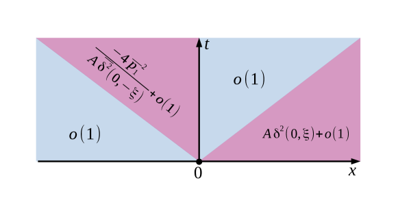
Under Assumptions (a)–(c), see Section 2.3, on the spectral functions associated with the initial data $q_{0}(x)$, the solution of the initial value problem (1.2), (1.3) has the following asymptotics as $t\to+\infty$, qualitatively different in sectors of the $(x,t)$ plane specified by ranges of $\xi=\frac{x}{4t}$:

$$q(x,t)=\left\{\begin{aligned} &A\delta^{2}(0,\xi)\prod\limits_{s=0}^{m-1}\left(\frac{\xi}{p_{n-s}}\right)^{2}+o(1),&-\mathop{\rm Re}\nolimits p_{n-m}<\xi<\omega_{n-m},\\ &o(1),&-\omega_{n-m}<\xi<\mathop{\rm Re}\nolimits p_{n-m},\\ &\frac{-4\overline{p}_{n-m}^{2}}{A\overline{\delta^{2}}(0,-\xi)}\prod\limits_{s=0}^{m-1}\left(\frac{\overline{p}_{n-s}}{\xi}\right)^{2}+o(1),&\mathop{\rm Re}\nolimits p_{n-m}<\xi<-\omega_{n-m-1},\\ &o(1),&\omega_{n-m-1}<\xi<-\mathop{\rm Re}\nolimits p_{n-m}.\end{aligned}\right.$$ (1.5)

Here $m=\overline{0,n-1}$, the function $\delta(0,\xi)$ and the numbers $\{p_{j}\}_{1}^{n}$ and $\{\omega_{j}\}_{1}^{n-1}$ ($p_{j}\in\mathbb{C}$ with $\mathop{\rm Im}\nolimits p_{j}>0$ and $\omega_{j}\in\mathbb{R}$) satisfying

$$-\infty<\mathop{\rm Re}\nolimits p_{n}<-\omega_{n-1}<\mathop{\rm Re}\nolimits p_{n-1}<-\omega_{n-2}<\dots<\mathop{\rm Re}\nolimits p_{1}<0$$

are determined in terms of the spectral functions associated with the initial data $q_{0}(x)$, see (3.4) and Assumptions (a)–(c). Particularly, in the case $n=1$, the principal asymptotic terms are as in Figure 1.

Refer to caption
Figure 1: Asymptotic behavior of the solution of problem (1.2), (1.3) satisfying Assumptions (a)-(c) with $n=1$.

Moreover, we are able to make this asymptotics more precise, either including in them a second term or writing explicitly a main decaying term for the corresponding sectors, see Theorem 2.

Our main tools used for obtaining these results are the inverse scattering transform (IST) method in the form of a Riemann-Hilbert (RH) problem and the subsequent use of the nonlinear steepest decent method (Deift and Zhou method; see [20, 16] and [18, 19, 40] for its extensions) for the large time analysis of the basic RH problem. Two main peculiarities of the adaptation of this approach to our problem are (i) the presence of a singularity on the contour for the original RH problem and (ii) the winding of the argument of certain spectral functions leading to a strong singularity on the contour for the “deformed RH problem” (needed for performing the long-time analysis, see (2.42) and (3.14) below).

The article is organized as follows. In Section 2 we present the implementation of the inverse scattering transform method for the initial value problem (1.2) in the form of a Riemann–Hilbert problem and examine the properties of the spectral functions associated to the initial data. A special attention is payed to the case of “pure step initial data”, i.e., for $q(x,0)=q_{R,A}(x)$, since this case provides ingredients guiding the study in the general case. The asymptotic analysis of the associated Riemann–Hilbert problem and the main result of the paper (Theorem 2) are presented in Section 3. In Section 4 we briefly discuss the asymptotics in the transition zones, and a short conclusion is given in Section 5.

2 Inverse scattering transform and the Riemann-Hilbert problem

The implementation of the Riemann-Hilbert problem approach to the step-like problems for local NLS equations substantially differs in the defocusing and focusing cases, due, in particular, to the fact that the structure of the spectrum of the associated differential operators (from the Lax pair representation) is different: either the whole spectrum is located on the real axis (defocusing case) or a part of it is outside this axis (focusing case). With this respect, we notice that the focusing and defocusing variants of the NNLS equation are closer to each other: in the both cases, (i) there is a point singularity on the real axis and (ii) the winding of the argument of certain spectral functions takes place, which affects the consequent asymptotic analysis. The next subsection presents the results of the direct scattering analysis for the both (focusing and defocusing) cases.

2.1 Direct scattering

As we have already mentioned, the NNLS equation (1.2a) is a compatibility condition of the system of two linear differential equations, the so-called Lax pair [4]:

$$\left\{\begin{array}[]{lcl}\Phi_{x}+ik\sigma_{3}\Phi=U(x,t)\Phi\\ \Phi_{t}+2ik^{2}\sigma_{3}\Phi=V(x,t,k)\Phi\\ \end{array}\right.$$ (2.1)

where $\sigma_{3}=\left(\begin{smallmatrix}1&0\\ 0&-1\end{smallmatrix}\right)$, $\Phi(x,t,k)$ is a $2\times 2$ matrix-valued function, $k\in\mathbb{C}$ is an auxiliary (spectral) parameter, and the matrix coefficients $U(x,t)$ and $V(x,t,k)$ can be written in terms of the solution $q(x,t)$ of the NNLS equation as follows:

$$U(x,t)=\begin{pmatrix}0&q(x,t)\\ -\sigma\bar{q}(-x,t)&0\\ \end{pmatrix},\qquad V=\begin{pmatrix}V_{11}&V_{12}\\ V_{21}&V_{22}\\ \end{pmatrix},$$ (2.2)

where $V_{11}=-V_{22}=i\sigma q(x,t)\bar{q}(-x,t)$, $V_{12}=2kq(x,t)+iq_{x}(x,t)$, $V_{21}=-2k\sigma\bar{q}(-x,t)+i\sigma(\bar{q}(-x,t))_{x}$.

Taking into account the boundary conditions (1.3) and assuming that the solution $q(x,t)$ of the problem (1.2) exists, we conclude that the matrices $U(x,t)$ and $V(x,t,k)$ converge to the following constant (w.r.t. $x$ and $t$) matrices (cf. [45]):

$$U(x,t)\rightarrow U_{\pm}\ \mbox{and}\ V(x,t,k)\rightarrow V_{\pm}(k)\quad\mbox{as}\ x\rightarrow\pm\infty,$$ (2.3)

where

$$U_{+}=\begin{pmatrix}0&A\\ 0&0\end{pmatrix},\,U_{-}=\begin{pmatrix}0&0\\ -\sigma A&0\end{pmatrix},\,V_{+}(k)=\begin{pmatrix}0&2kA\\ 0&0\end{pmatrix},\,V_{-}(k)=\begin{pmatrix}0&0\\ -2\sigma kA&0\end{pmatrix}.$$ (2.4)

Notice that the system (2.1) is compatible with $U_{+}$, $V_{+}$ or $U_{-}$, $V_{-}$ used instead of $U$ and $V$, so the boundary conditions (1.3)1.3(\ref{2}) are meaningful for the NNLS equations (in contrast with their local counterparts, where the boundary conditions have to be exact solutions depending on $x$ and $t$).

Introduce the “background solutions” $\Phi_{\pm}$ which are the solutions of the system (2.1) with $U(x,t)$ and $V(x,t,k)$ replaced by $U_{\pm}$ and $V_{\pm}$ respectively:

$$\Phi_{\pm}(x,t,k)=N_{\pm}(k)e^{-(ikx+2ik^{2}t)\sigma_{3}},$$ (2.5)

where $N_{+}(k)=\begin{pmatrix}1&\frac{A}{2ik}\\ 0&1\end{pmatrix},\,N_{-}(k)=\begin{pmatrix}1&0\\ \frac{\sigma A}{2ik}&1\end{pmatrix}.$ Similarly to the case of the focusing NNLS equation [45, 46], $N_{\pm}(k)$ have singularities at $k=0$, which play a significant role in the analysis (see the basic Riemann-Hilbert problem in Section 2.3 below).

Next define the $2\times 2$-valued functions $\Psi_{j}(x,t,k)$, $j=1,2$, $x\in\mathbb{R}$, $t\geq 0$ as the solutions of the linear Volterra integral equations:

$\displaystyle\Psi_{1}(x,t,k)=N_{-}(k)+\int^{x}_{-\infty}G_{-}(x,y,t,k)\left(U(y,t)-U_{-}\right)\Psi_{1}(y,t,k)e^{ik(x-y)\sigma_{3}}\,dy,\,k\in(\mathbb{C}^{+},\mathbb{C}^{-}),$ (2.6a)
$\displaystyle\Psi_{2}(x,t,k)=N_{+}(k)-\int_{x}^{\infty}G_{+}(x,y,t,k)\left(U(y,t)-U_{+}\right)\Psi_{2}(y,t,k)e^{ik(x-y)\sigma_{3}}\,dy,\,k\in(\mathbb{C}^{-},\mathbb{C}^{+}),$ (2.6b)

where the Cauchy matrices $G_{\pm}(x,y,t,k)$ have the form

$$G_{\pm}(x,y,t,k)=\Phi_{\pm}(x,t,k)[\Phi_{\pm}(y,t,k)]^{-1},$$ (2.7)

and $\mathbb{C}^{\pm}=\left\{k\in\mathbb{C}\,|\pm\mathop{\rm Im}\nolimits k>0\right\}$. Here and below, the notation $k\in(\mathbb{C}^{+},\mathbb{C}^{-})$ ($k\in(\mathbb{C}^{-},\mathbb{C}^{+})$), means that the first and the second column of the relevant matrix can be analytically continued from the real axis into respectively the upper (lower) and lower (upper) half-plane as bounded functions. The functions $\Psi_{j}(x,t,k)$, $j=1,2$, play a significant role in the analysis, namely, they are the key elements in the construction of the basic Riemann-Hilbert problem (see Section 2.3 below). We summarize their main properties (cf. [45]) in

Proposition 1.

The $2\times 2$-valued matrix functions $\Psi_{j}(x,t,k)$, $j=1,2$ (see 2.6) have the following properties:

  1. (i)

    The functions

    $$\Phi_{j}(x,t,k):=\Psi_{j}(x,t,k)e^{-(ikx+2ik^{2}t)\sigma_{3}},\quad k\in\mathbb{R}\setminus\{0\},\quad j=1,2,$$ (2.8)

    are the Jost solutions of the system (2.1) satisfying the boundary conditions (see (2.5))

    $$\Phi_{1}(x,t,k)\to\Phi_{-}(x,t,k)\ \ \text{as}\ x\to-\infty,\quad\Phi_{2}(x,t,k)\to\Phi_{+}(x,t,k)\ \ \text{as}\ x\to+\infty.$$
  2. (ii)

    $\det\Psi_{j}(x,t,k)=1,\quad x,k\in\mathbb{R},\,t\geq 0,\quad j=1,2.$

  3. (iii)

    The symmetry property:

    $$\Lambda\overline{\Psi_{1}(-x,t,-k)}\Lambda^{-1}=\Psi_{2}(x,t,k),\quad k\in\mathbb{R}\setminus\{0\},$$ (2.9)

    where $\Lambda=\begin{pmatrix}0&\sigma\\ 1&0\end{pmatrix}$.

  4. (iv)

    As $k\to 0$, the columns $\Psi_{j}^{(1)}(x,t,k)$ and $\Psi_{j}^{(2)}(x,t,k)$ of $\Psi_{j}(x,t,k)$, $j=1,2$ behave as follows:

    $\displaystyle\Psi_{1}^{(1)}(x,t,k)=\frac{1}{k}\begin{pmatrix}v_{1}(x,t)\\ v_{2}(x,t)\end{pmatrix}+O(1),$ $\displaystyle\Psi_{1}^{(2)}(x,t,k)=\frac{2i\sigma}{A}\begin{pmatrix}v_{1}(x,t)\\ v_{2}(x,t)\end{pmatrix}+O(k),$ (2.10a)
    $\displaystyle\Psi_{2}^{(1)}(x,t,k)=-\frac{2i}{A}\begin{pmatrix}\sigma\overline{v_{2}}(-x,t)\\ \overline{v_{1}}(-x,t)\end{pmatrix}+O(k),$ $\displaystyle\Psi_{2}^{(2)}(x,t,k)=-\frac{1}{k}\begin{pmatrix}\sigma\overline{v_{2}}(-x,t)\\ \overline{v_{1}}(-x,t)\end{pmatrix}+O(1),$ (2.10b)

    where $v_{1}(x,t)$ and $v_{2}(x,t)$ are some functions.

Proof.

Item $(i)$ can be verified directly from the definition of $\Psi_{j}(x,t,k)$ (see (2.6)). Item $(ii)$ follows from the facts that (a) $\det\Phi_{j}(x,t,k)=\det\Psi_{j}(x,t,k)$ for $x,k\in\mathbb{R}$ and $t\geq 0$ and (b) $U(x,t)$ and $V(x,t)$ are traceless matrices. Item $(iii)$ follows from the symmetry $\Lambda\overline{U(-x,t)}\Lambda^{-1}=U(x,t).$

Concerning item $(iv)$, we observe that the structure of the singularity of $N_{\pm}(k)$ as $k\to 0$ and the definition of $\Psi_{j}(x,t,k)$, $j=1,2$ imply that, as $k\to 0$,

$\displaystyle\Psi_{1}^{(1)}(x,t,k)=\frac{1}{k}\begin{pmatrix}v_{1}(x,t)\\ v_{2}(x,t)\end{pmatrix}+O(1),$ $\displaystyle\Psi_{1}^{(2)}(x,t,k)=\begin{pmatrix}\tilde{v}_{1}(x,t)\\ \tilde{v}_{2}(x,t)\end{pmatrix}+O(k),$ (2.11a)
$\displaystyle\Psi_{2}^{(1)}(x,t,k)=\begin{pmatrix}\tilde{w}_{1}(x,t)\\ \tilde{w}_{2}(x,t)\end{pmatrix}+O(k),$ $\displaystyle\Psi_{2}^{(2)}(x,t,k)=\frac{1}{k}\begin{pmatrix}w_{1}(x,t)\\ w_{2}(x,t)\end{pmatrix}+O(1).$ (2.11b)

Then, from the symmetry relation (2.9) it follows that

$$\begin{pmatrix}w_{1}(x,t)\\ w_{2}(x,t)\end{pmatrix}=\begin{pmatrix}-\sigma\overline{v_{2}}(-x,t)\\ -\overline{v_{1}}(-x,t)\end{pmatrix}\quad\text{and}\quad\begin{pmatrix}\tilde{w}_{1}(x,t)\\ \tilde{w}_{2}(x,t)\end{pmatrix}=\begin{pmatrix}\overline{\tilde{v}_{2}}(-x,t)\\ \sigma\overline{\tilde{v}_{1}}(-x,t)\end{pmatrix}.$$ (2.12)

Further, substituting (2.11a) into (2.6a) we conclude that $v_{j}(x,t)$, $j=1,2$ satisfy the system of integral equations

$$\begin{cases}v_{1}(x,t)=\int_{-\infty}^{x}q(y,t)v_{2}(y,t)\,dy,\\ v_{2}(x,t)=-i\sigma\frac{A}{2}-\sigma\int_{-\infty}^{x}\overline{q(-y,t)}v_{1}(y,t)\,dy.\end{cases}$$ (2.13)

whereas $\tilde{v}_{j}(x,t)$, $j=1,2$ solve the following system of equations:

$$\begin{cases}\tilde{v}_{1}(x,t)=\int_{-\infty}^{x}q(y,t)\tilde{v}_{2}(y,t)\,dy,\\ \tilde{v}_{2}(x,t)=1-\sigma\int_{-\infty}^{x}\overline{q(-y,t)}\tilde{v}_{1}(y,t)\,dy.\end{cases}$$ (2.14)

Comparing (2.13) with (2.14) it follows that

$$\begin{pmatrix}\tilde{v}_{1}(x,t)\\ \tilde{v}_{2}(x,t)\end{pmatrix}=\frac{2i\sigma}{A}\begin{pmatrix}v_{1}(x,t)\\ v_{2}(x,t)\end{pmatrix}.$$

Since the Jost solutions $\Phi_{1}(x,t,k)$ and $\Phi_{2}(x,t,k)$ defined by (2.8) satisfy the system (2.1) for all $k\in\mathbb{R}\setminus\{0\}$, they are related by a matrix function independent of $x$ and $t$:

$$\Phi_{1}(x,t,k)=\Phi_{2}(x,t,k)S(k),\quad k\in\mathbb{R}\setminus\{0\},$$ (2.15)

or, in terms of $\Psi_{j}(x,t,k)$, $j=1,2$

$$\Psi_{1}(x,t,k)=\Psi_{2}(x,t,k)e^{-(ikx+2ik^{2}t)\sigma_{3}}S(k)e^{(ikx+2ik^{2}t)\sigma_{3}},\,\,k\in\mathbb{R}\setminus\{0\},$$ (2.16)

where $S(k)$ is the so-called scattering matrix. Due to the symmetry (2.9) the matrix $S(k)$ can be written as follows (cf. [45])

$$S(k)=\begin{pmatrix}a_{1}(k)&-\sigma\overline{b(-k)}\\ b(k)&a_{2}(k)\end{pmatrix},\qquad k\in\mathbb{R}\setminus\{0\},$$ (2.17)

with some functions (the so-called spectral functions) $b(k)$ and $a_{j}(k)$, $j=1,2$, which satisfy the symmetry relation $\overline{a_{j}(-k)}=a_{j}(k)$, $j=1,2$. The spectral functions can be obtained in terms of the initial data only:

$$S(k)=\Psi_{2}^{-1}(0,0,k)\Psi_{1}(0,0,k),$$ (2.18)

or, alternatively, by using the determinant relations

$\displaystyle b(k)$ $\displaystyle=\det\left(\Psi_{2}^{(1)}(0,0,k),\Psi_{1}^{(1)}(0,0,k)\right),\quad k\in\mathbb{R},$ (2.19a)
$\displaystyle a_{1}(k)$ $\displaystyle=\det\left(\Psi_{1}^{(1)}(0,0,k),\Psi_{2}^{(2)}(0,0,k)\right),\quad k\in\overline{\mathbb{C}^{+}}\setminus\{0\},$ (2.19b)
$\displaystyle a_{2}(k)$ $\displaystyle=\det\left(\Psi_{2}^{(1)}(0,0,k),\Psi_{1}^{(2)}(0,0,k)\right),\quad k\in\overline{\mathbb{C}^{-}}.$ (2.19c)

We summarize the properties of the spectral functions $b(k)$ and $a_{j}(k)$, $j=1,2$ in the following proposition (cf. [45]; particularly, item 5 below follows from (2.10)):

Proposition 2.

The spectral functions $b(k)$, $a_{j}(k)$, $j=1,2$, have the following properties

  1. 1.

    $a_{1}(k)$ is analytic in $k\in\mathbb{C}^{+}$ and continuous in $\overline{\mathbb{C}^{+}}\setminus\{0\}$; $a_{2}(k)$ is analytic in $k\in\mathbb{C}^{-}$ and continuous in $\overline{\mathbb{C}^{-}}$.

  2. 2.

    $a_{j}(k)=1+{O}\left(\frac{1}{k}\right)$, $j=1,2$ and $b(k)={O}\left(\frac{1}{k}\right)$ as $k\rightarrow\infty$ (the latter holds for $k\in{\mathbb{R}}$).

  3. 3.

    $\overline{a_{1}(-\bar{k})}=a_{1}(k)$, $k\in\overline{\mathbb{C}^{+}}\setminus\{0\}$;   $\overline{a_{2}(-\bar{k})}=a_{2}(k)$, $k\in\overline{\mathbb{C}^{-}}$.

  4. 4.

    $a_{1}(k)a_{2}(k)+\sigma b(k)\overline{b(-\bar{k})}=1$, $k\in{\mathbb{R}}\setminus\{0\}$ (follows from $\det S(k)=1$).

  5. 5.

    As $k\to 0$, $a_{1}(k)=\sigma\frac{A^{2}a_{2}(0)}{4k^{2}}+O\left(\frac{1}{k}\right)$ and $b(k)=\sigma\frac{Aa_{2}(0)}{2ik}+O\left(1\right)$.

2.2 Spectral functions for the “shifted step” initial data

Henceforth, we deal with the defocusing NNLS equation (making comparisons, if appropriate, with the case of the focusing NNLS equation). Analytic considerations in the case of pure step initial data (1.4) presented below will guide us in establishing the general framework suitable for the asymptotic analysis.

The spectral functions associated with the initial data $q_{0}(x)=q_{R,A}(x)$ are given explicitly by

$\displaystyle a_{1}(k)=1-\frac{A^{2}}{4k^{2}}e^{4ikR},$ (2.20a)
$\displaystyle a_{2}(k)=1,$ (2.20b)
$\displaystyle b(k)=-\frac{A}{2ik}e^{2ikR}.$ (2.20c)

Indeed, the scattering matrix $S(k)$ can be obtained from (2.16) taking $x=-R$ and $t=0$:

$$S(k)=e^{-ikR\sigma_{3}}\Psi_{2}^{-1}(-R,0,k)\Psi_{1}(-R,0,k)e^{ikR\sigma_{3}}.$$ (2.21)

It follows from (2.6) at $t=0$ that

$\displaystyle\Psi_{1}(-R,0,k)=N_{-}(k),$ (2.22a)
$\displaystyle\Psi_{2}(-R,0,k)=N_{+}(k)-\int^{R}_{-R}G_{+}(-R,y,0,k)\begin{pmatrix}0&-A\\ 0&0\end{pmatrix}\Psi_{2}(y,0,k)e^{-ik(R+y)\sigma_{3}}\,dy,$ (2.22b)

where $\Psi_{2}(x,0,k)$ for $x\in\left[-R,R\right]$ solves the integral equation

$$\Psi_{2}(x,0,k)=N_{+}(k)-\int^{R}_{x}G_{+}(x,y,0,k)\begin{pmatrix}0&-A\\ 0&0\end{pmatrix}\Psi_{2}(y,0,k)e^{ik(x-y)\sigma_{3}}\,dy,\quad x\in[-R,R].$$ (2.23)

From the definition of $G_{+}$ (see (2.7)) it follows that

$$G_{+}(x,y,0,k)=\begin{pmatrix}e^{-ik(x-y)}&\frac{A}{2ik}\left(e^{ik(x-y)}-e^{-ik(x-y)}\right)\\ 0&e^{ik(x-y)}\end{pmatrix},$$

and then direct calculations show that the solution of the equation (2.23) is as follows:

$$\Psi_{2}(x,0,k)=\begin{pmatrix}1&\frac{A}{2ik}e^{2ik(R-x)}\\ 0&1\end{pmatrix},\quad x\in\left[-R,R\right].$$ (2.24)

Substituting (2.22) and (2.24) into (2.21) we arrive at (2.20).

Now let us analyze the locations of zeros of $a_{1}(k)$ in $\overline{{\mathbb{C}^{+}}}$ and the behavior of its argument for $k\in\mathbb{R}$.

Proposition 3.
  1. (i)

    For $\frac{(n-1)\pi}{A}<R<\frac{n\pi}{A}$, $n\in\mathbb{N}$, $a_{1}(k)$ has the following properties:

    • $a_{1}(k)$ has $2n$ simple zeros in $\overline{\mathbb{C}^{+}}$: $\{p_{j},-\overline{p}_{j}\}_{j=1}^{n}$. Here $\{\mathop{\rm Re}\nolimits p_{j}\}_{j=1}^{n}$ are the ordered set of solutions of the equations

      $$k=\pm\frac{A}{2}\cos(2kR)e^{-2kR\tan(2kR)},$$ (2.25)

      considered for $k<0$, and $\mathop{\rm Im}\nolimits p_{j}$ and $\mathop{\rm Re}\nolimits p_{j}$ are related by

      $$\mathop{\rm Im}\nolimits p_{j}=\mathop{\rm Re}\nolimits p_{j}\tan(2\mathop{\rm Re}\nolimits p_{j}R),\quad j=\overline{1,n}.$$ (2.26)

      Notice that

      $$\mathop{\rm Re}\nolimits p_{j}\in\left(-\frac{(2j-1)\pi}{4R},-\frac{(j-1)\pi}{2R}\right),\quad j=\overline{1,n}$$ (2.27)

      and that behavior of the real and imaginary parts of the zeros $p_{j}$ as $R$ increases is similar to the case of the focusing NNLS equation [46].

    • Define $\omega_{j}$, $j=\overline{0,n}$ as follows: $\omega_{0}=0$, $\omega_{j}=\frac{j\pi}{2R}$ for $j=\overline{1,n-1}$, and $\omega_{n}=\infty$. Then

      $\displaystyle\int_{-\infty}^{-\omega_{n-j}}d\arg a_{1}(k)=(2j-1)\pi,\quad j=\overline{1,n-1},$ (2.28a)
      $\displaystyle\int_{-\infty}^{-\xi}d\arg a_{1}(k)\in((2j-1)\pi,(2j+1)\pi),\quad-\omega_{n-j}<-\xi<-\omega_{n-j-1},\quad j=\overline{0,n-1}.$ (2.28b)
  2. (ii)

    If $R=\frac{n\pi}{A}$ for some $n\in\mathbb{N}\cup\{0\}$, then $a_{1}(k)$ has $2n+2$ simple zeros in $\overline{\mathbb{C}^{+}}$ at $\{\pm\frac{A}{2}$, $\{p_{j},-\overline{p}_{j}\}_{j=1}^{n}\}$, where $\mathop{\rm Re}\nolimits p_{j}$ ($j=\overline{1,n}$) are the solutions of (2.25), and $\mathop{\rm Im}\nolimits p_{j}$ are determined by (2.26).

Proof.

Observe that the equation $a_{1}(k)=0$ is equivalent to the system

$$\begin{cases}k_{1}=\pm\frac{A}{2}\cos(2k_{1}R)e^{-2k_{2}R}\\ k_{2}=\pm\frac{A}{2}\sin(2k_{1}R)e^{-2k_{2}R}\end{cases},$$ (2.29)

where $k=k_{1}+ik_{2}$, $k\in\overline{\mathbb{C}^{+}}\setminus\{0\}$. Due to the symmetry relation $a_{1}(k)=\overline{a_{1}(-\bar{k})}$ it is sufficient to consider (2.29) for $k_{1}\geq 0$ only.

(i) For $k_{1}=0$, the system (2.29) clearly has no solutions, so $a_{1}(k)$ has no purely imaginary zeros (notice that in the focusing case, $a_{1}(k)$ has one simple purely imaginary zero [46]).

(ii) Assuming $k_{2}=0$, the second equation in (2.29) implies that $k_{1}$ must be equal to $\frac{\pi n}{2R}$ with some $n\in\mathbb{N}$. But then, from the first equation in (2.29) we conclude that $k_{1}=\frac{A}{2}$. Therefore, $k=\pm\frac{A}{2}$ are simple zeros of $a_{1}(k)$ if and only if there exists $n\in\mathbb{N}$ such that $\pi n=AR$. Notice that in the case $R=0$, the spectral function $a_{1}(k)$ has exactly two simple zeros, $\frac{A}{2}$ and $-\frac{A}{2}$.

(iii) Now, let’s look at the location of zeros of $a_{1}(k)$ in the open quarter plane $k_{1}>0$, $k_{2}>0$. Dividing the equations in (2.29) sidewise we arrive at (cf. (2.26))

$$k_{2}=k_{1}\tan(2k_{1}R),\quad k_{1}\neq\frac{\pi(2n+1)}{4R},\,n\in\mathbb{N},$$ (2.30)

from which we conclude (cf. (2.27)) that

$$k_{1}\in\left(\frac{(n-1)\pi}{2R},\frac{(2n-1)\pi}{4R}\right),\quad n\in\mathbb{N}.$$ (2.31)

Substituting (2.30) into the first equation in (2.29) and taking into account the sign of $\cos(2k_{1}R)$ for $k_{1}$ satisfying (2.31), we obtain the equations for $k_{1}$:

$$k_{1}=\frac{A}{2}\cos(2k_{1}R)e^{-2k_{1}R\tan(2k_{1}R)}\quad\text{for}\ k_{1}\in\left(\frac{(n-1)\pi}{R},\frac{(4n-3)\pi}{4R}\right),\quad n\in\mathbb{N},$$ (2.32a)
or
$$k_{1}=-\frac{A}{2}\cos(2k_{1}R)e^{-2k_{1}R\tan(2k_{1}R)}\quad\text{for}\ k_{1}\in\left(\frac{(2n-1)\pi}{2R},\frac{(4n-1)\pi}{4R}\right),\quad n\in\mathbb{N}.$$ (2.32b)

Since the r.h.s. of (2.32a) and (2.32b) monotonically decrease w.r.t. $k_{1}$ in the corresponding intervals, it follows that for $\frac{(n-1)\pi}{A}<R\leq\frac{n\pi}{A}$ equations (2.32) have $n$ simple solutions $\{k_{1,j}\}_{j=1}^{n}$ in the quarter plane $k_{1}>0$, $k_{2}>0$ such that $k_{1,j}\in\left(\frac{(j-1)\pi}{2R},\frac{(2j-1)\pi}{4R}\right)$, $j=\overline{1,n}$ (cf. (2.27)).

Concerning the winding properties of $\arg a_{1}(k)$, the estimates (for $\frac{(n-1)\pi}{A}<R<\frac{n\pi}{A}$)

$\displaystyle\frac{A^{2}}{4k_{(m)}^{2}}e^{4ik_{(m)}R}<1\quad\text{for}\ k_{(m)}=-\frac{m\pi}{2R},\quad m\in\mathbb{N},\quad m\geq n,$ (2.33a)
$\displaystyle\frac{A^{2}}{4k_{(m)}^{2}}e^{4ik_{(m)}R}>1\quad\text{for}\ k_{(m)}=-\frac{m\pi}{2R},\quad m\in\mathbb{N},\quad m<n,$ (2.33b)

yield (2.28). ∎

Remark 1.

Considering the pure step initial data $q_{R,A}$ as varying with $R$ (for a fixed $A$), the values $R=\frac{n\pi}{A}$, $n=0,1,2,\dots$ turn to be the bifurcation points: when $R$ is passing any of these values, $a_{1}(k)$ acquires an additional pair of zeros at $k=\pm\frac{A}{2}$ (cf. [10], Section 4.1, where the box-type piecewise-constant initial data for the defocusing NLS equation with nonzero boundary conditions at infinity are considered illustrating the bifurcation of discrete eigenvalues).

2.3 The basic Riemann-Hilbert problem and inverse scattering

One of the main advantages of the Riemann-Hilbert approach in the Inverse Scattering Transform method is that it is highly efficient in the asymptotic analysis. Recall that the Riemann-Hilbert (RH) problem (as widely used in applications to integrable systems) consists in finding an $n\times n$-valued piece-wise meromorphic function that satisfies a prescribed jump condition across a contour in the complex plane and prescribed conditions at singular points (if any). The jump matrix for RH problems associated with initial (and initial-boundary) value problems for integrable systems are usually oscillatory with respect to a large parameter (in our case, time); in treating (asymptotically) these problems, the so-called nonlinear steepest decent method (Deift and Zhou method [20]) has proved to be extremely efficient.

The construction of the RH problem for an integrable system is usually based (at least in the case when the differential equations in the Lax pair representation are of the second order), on analytic properties of the Jost solutions $\Phi_{j}(x,t,k)$ and, correspondingly, the functions $\Psi_{j}(x,t,k)$. Similarly to the case of the focusing NNLS equation [45, 46], we define the $2\times 2$-valued, piece-wise meromorphic (relative to the real line) function $M(x,t,k)$ by

$$M(x,t,k)=\left\{\begin{array}[]{lcl}\left(\frac{\Psi_{1}^{(1)}(x,t,k)}{a_{1}(k)},\Psi_{2}^{(2)}(x,t,k)\right),\quad k\in\mathbb{C}^{+},\\ \left(\Psi_{2}^{(1)}(x,t,k),\frac{\Psi_{1}^{(2)}(x,t,k)}{a_{2}(k)}\right),\quad k\in\mathbb{C}^{-}.\\ \end{array}\right.$$ (2.34)

The scattering relation (2.16) implies that the boundary values $M_{\pm}(x,t,k)=\underset{k^{\prime}\to k,k^{\prime}\in{\mathbb{C}}^{\pm}}{\lim}M(x,t,k^{\prime})$, $k\in\mathbb{R}$ (we take the non-tangential limits) satisfy the jump condition

$$M_{+}(x,t,k)=M_{-}(x,t,k)J(x,t,k),\qquad k\in\mathbb{R}\setminus\{0\}$$ (2.35)

with the jump matrix

$$J(x,t,k)=\begin{pmatrix}1-r_{1}(k)r_{2}(k)&-r_{2}(k)e^{-2ikx-4ik^{2}t}\\ r_{1}(k)e^{2ikx+4ik^{2}t}&1\end{pmatrix},$$ (2.36)

where the reflection coefficients $r_{1}(k)$, $j=1,2$ are defined by

$$r_{1}(k):=\frac{b(k)}{a_{1}(k)},\quad r_{2}(k):=\frac{\overline{b(-k)}}{a_{2}(k)}.$$ (2.37)

Observe that from the determinant relation (see item 4 with $\sigma=-1$ in Proposition 2) we have

$$1-r_{1}(k)r_{2}(k)=\frac{1}{a_{1}(k)a_{2}(k)}.$$ (2.38)

Moreover,

$$M(x,t,k)\to I,\qquad k\to\infty,$$ (2.39)

where $I$ is the $2\times 2$ identity matrix.

Taking into account the singularities of $\Psi_{j}(x,t,k)$, $j=1,2$ and $a_{1}(k)$ at $k=0$ (see Propositions 1 and 2), the function $M(x,t,k)$ has the following behavior as $k\to 0$:

$\displaystyle M(x,t,k)=\begin{pmatrix}-\frac{4}{A^{2}a_{2}(0)}v_{1}(x,t)&\overline{v_{2}}(-x,t)\\ -\frac{4}{A^{2}a_{2}(0)}v_{2}(x,t)&-\overline{v_{1}}(-x,t)\end{pmatrix}(I+O(k))\begin{pmatrix}k&0\\ 0&\frac{1}{k}\end{pmatrix},$ $\displaystyle k\rightarrow 0,\quad k\in\mathbb{C}^{+},$ (2.40a)
$\displaystyle M(x,t,k)=\frac{2i}{A}\begin{pmatrix}\overline{v_{2}}(-x,t)&-\frac{v_{1}(x,t)}{a_{2}(0)}\\ -\overline{v_{1}}(-x,t)&-\frac{v_{2}(x,t)}{a_{2}(0)}\end{pmatrix}+O(k),$ $\displaystyle k\rightarrow 0,\quad k\in\mathbb{C}^{-},$ (2.40b)

where $v_{j}(x,t)$, $j=1,2$ are some functions.

Similarly to the focusing NNLS equation [46], the properties of $a_{j}(k)$, $j=1,2$ in the case of the “shifted step” initial data (see Proposition 3) guide us to make assumptions on the spectral functions $a_{j}(k)$, $j=1,2$ associated with initial data satisfying (1.2c). We emphasize that these assumptions differ from those made in the focusing case (particularly, the order of $\mathop{\rm Re}\nolimits p_{j}$ and $\omega_{j}$ is different, see (2.41) below), which significantly affects the resulting asymptotic formulas.

Assumptions:

(a) $a_{1}(k)$ has $2n$, $n\in\mathbb{N}$, simple zeros in $\overline{{\mathbb{C}}^{+}}\setminus\{0\}$, $\{p_{j}\}_{j=1}^{n}$ and $\{-\overline{p}_{j}\}_{j=1}^{n}$, with $\mathop{\rm Im}\nolimits p_{j}>0$ and $\mathop{\rm Re}\nolimits p_{n}<\dots<\mathop{\rm Re}\nolimits p_{1}<0$.

(b) $a_{2}(k)$ has no zeros in $\overline{\mathbb{C}^{-}}$.

(c) There exist numbers $\omega_{m}>0$, $m=\overline{1,n-1}$ such that

$$-\infty<\mathop{\rm Re}\nolimits p_{n}<-\omega_{n-1}<\mathop{\rm Re}\nolimits p_{n-1}<-\omega_{n-2}<\dots<\mathop{\rm Re}\nolimits p_{1}<0,$$ (2.41)
$$\int_{-\infty}^{-\omega_{n-m}}d\arg\left(a_{1}(k)a_{2}(k)\right)=(2m-1)\pi,\quad m=\overline{1,n-1},$$ (2.42a)
and
$$\int_{-\infty}^{-\xi}d\arg\left(a_{1}(k)a_{2}(k)\right)\in((2m-1)\pi,(2m+1)\pi),\quad-\omega_{n-m}<-\xi<-\omega_{n-m-1},\quad m=\overline{0,n-1}$$ (2.42b)
(here we adopt the notations $\omega_{0}=0$ and $\omega_{n}=+\infty$).

The construction of $M$ implies that at the zeros of $a_{1}(k)$, $M(x,t,k)$ satisfies the following residue conditions:

$\displaystyle\underset{k=p_{j}}{\operatorname{Res}}M^{(1)}(x,t,k)$ $\displaystyle=\frac{\eta_{j}}{\dot{a}_{1}(p_{j})}e^{2ip_{j}x+4ip_{j}^{2}t}M^{(2)}(x,t,p_{j}),\quad j=\overline{1,n},$ (2.43a)
$\displaystyle\underset{k=-\overline{p}_{j}}{\operatorname{Res}}M^{(1)}(x,t,k)$ $\displaystyle=\frac{1}{\bar{\eta}_{j}\dot{a}_{1}(-\overline{p}_{j})}e^{-2i\overline{p}_{j}x+4i\overline{p}_{j}^{2}t}M^{(2)}(x,t,-\overline{p}_{j}),\quad j=\overline{1,n}.$ (2.43b)

Here $\eta_{j}$, $j=\overline{1,n}$ are constants determined by the initial data through $\Psi_{1}^{(1)}(0,0,p_{j})=\eta_{j}\Psi_{2}^{(2)}(0,0,p_{j})$.

Basing on the analytic properties of $M$ presented above, we observe that we can characterize $M$ as the solution of a Riemann–Hilbert problem, with data uniquely determined by the initial data $q_{0}(x)$, in terms of the associated spectral data.

Basic Riemann–Hilbert Problem:

Given $b(k)$, $k\in{\mathbb{R}}$ and $a_{j}(k)$, $j=1,2$ which satisfy properties 1-5 in Proposition 2 and assumptions (a)-(c) above, and constants $\eta_{j}$, $j=\overline{1,n}$, find the $2\times 2$-valued, piece-wise (relative to $\mathbb{R}$) meromorphic in $k$ function $M(x,t,k)$ satisfying the following conditions:

(1)

The jump condition:

$$M_{+}(x,t,k)=M_{-}(x,t,k)J(x,t,k),\qquad k\in\mathbb{R}\setminus\{0\}$$ (2.44)

with the jump matrix $J(x,t,k)$ given by (2.36), where $r_{j}(k)$, $j=1,2$ are determined in terns of $b(k)$ and $a_{j}(k)$, $j=1,2$ by (2.37).

(2)

The residue conditions (2.43).

(3)

The pseudo-residue conditions (2.40) at $k=0$, where $v_{j}(x,t)$, $j=1,2$ are not prescribed.

(4)

The normalization condition at $k=\infty$:

$$M(x,t,k)=I+O(k^{-1})\quad\mbox{uniformly as }k\to\infty.$$

Assuming that the Riemann-Hilbert problem (1)–(4) has a solution $M(x,t,k)$, the solution of the initial value problem (1.2), (1.3) can be expressed as follows:

$$q(x,t)=2i\lim_{k\to\infty}kM_{12}(x,t,k)$$ (2.45)

or

$$q(-x,t)=-2i\lim_{k\to\infty}k\overline{M_{21}(x,t,k)}.$$ (2.46)
Remark 2.

The solution of Basic Riemann-Hilbert Problem is unique. Indeed, let $M$ and $\tilde{M}$ be two solutions of the problem, then $M\tilde{M}^{-1}$ has no jump across $\mathbb{R}\setminus\{0\}$ and it is bounded at $k=0$ (which can be seen from (2.40)), $k=p_{j}$ and $k=-\bar{p}_{j}$. Taking into account the normalization condition (4), by the Liouville theorem it follows that $M\tilde{M}^{-1}\equiv I$.

Remark 3.

(2.45) and (2.46) imply that the solution of problem (1.2), (1.3) for all $x\in(-\infty,\infty)$ can be expressed in terms of the solutions of the RH problems evaluated for $x\geq 0$ only.

Remark 4.

In contrast with local integrable equations, where zeros of certain spectral functions (analogues of $a_{j}(k)$, $j=1,2$) are associated with solitons traveling on a prescribed background (even in the cases when the background is nonzero), for nonlocal equations, certain number of zeros of $a_{j}(k)$, $j=1,2$ is always associated with the background itself. In the present paper, we restrict ourselves to the case without additional zeros (associated with the deflection of $q_{0}(x)$ from the background (1.4).

3 The long-time asymptotics

In the present section we study the long-time behavior of the solution of the initial value problem (1.2), (1.3) under Assumptions (a)-(c). For this purpose, we adapt the nonlinear steepest-decent method [20] to Basic Riemann-Hilbert Problem (1)–(4) (see Section 2.3).

3.1 Jump factorizations

Introducing the phase function

$$\theta(k,\xi)=4k\xi+2k^{2}$$ (3.1)

in terms of the slow variable $\xi=\frac{x}{4t}$, the jump matrix (2.36) admits the triangular factorizations of two types [45, 46]:

$\displaystyle J(x,t,k)$ $\displaystyle=\begin{pmatrix}1&0\\ \frac{r_{1}(k)}{1-r_{1}(k)r_{2}(k)}e^{2it\theta}&1\\ \end{pmatrix}\begin{pmatrix}1-r_{1}(k)r_{2}(k)&0\\ 0&\frac{1}{1-r_{1}(k)r_{2}(k)}\\ \end{pmatrix}\begin{pmatrix}1&\frac{-r_{2}(k)}{1-r_{1}(k)r_{2}(k)}e^{-2it\theta}\\ 0&1\\ \end{pmatrix}$ (3.2a)
$\displaystyle=\begin{pmatrix}1&-r_{2}(k)e^{-2it\theta}\\ 0&1\\ \end{pmatrix}\begin{pmatrix}1&0\\ r_{1}(k)e^{2it\theta}&1\\ \end{pmatrix}.$ (3.2b)

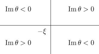
The idea of the nonlinear steepest descent method is to transform the original RH problem to such a form, where the jump matrix converges rapidly to $I$ away from a vicinity of the stationary phase point $k=-\xi$ of $\theta$. Since $\theta(k,\xi)$ and its signature table (see Figure 2) are the same as in the case of the local NLS equation, we can initiate the RH problem transformations similarly to the local case, introducing an auxiliary scalar function $\delta(k,\xi)$ in order to get rid of the diagonal factor in (3.2a). This function can be defined as the solution of the following scalar RH problem:

$\displaystyle\delta_{+}(k,\xi)=\delta_{-}(k,\xi)(1-r_{1}(k)r_{2}(k)),$ $\displaystyle k\in(-\infty,-\xi),$ (3.3a)
$\displaystyle\delta(k,\xi)\rightarrow 1,$ $\displaystyle k\rightarrow\infty.$ (3.3b)

Although problem (3.3) seems to be exactly the same as in the case of the local NLS [16], a principal difference is that the jump $(1-r_{1}(k)r_{2}(k))$ is, in general, a complex-valued function, which can lead to a strong singularity at $k=-\xi$. In order to cope with the similar problem in the focusing case, in [46] we introduced a finite number of “partial functions delta”, which have weak singularities, and proceed with their product. Here we proceed in a different way, defining a single function $\delta(k,\xi)$ as the solution of the scalar RH problem (3.3), and then dealing with the strong singularity at $k=-\xi$.

Refer to caption
Figure 2: Signature table

The function $\delta(k,\xi)$ given by the Cauchy integral

$$\delta(k.\xi)=\exp\left\{\frac{1}{2\pi i}\int_{-\infty}^{-\xi}\frac{\ln(1-r_{1}(\zeta)r_{2}(\zeta))}{\zeta-k}\,d\zeta\right\}$$ (3.4)

satisfies (3.3) and can be written as

$$\delta(k,\xi)=(k+\xi)^{i\nu(-\xi)}e^{\chi(k,\xi)},$$ (3.5)

where

$$\chi(k,\xi)=-\frac{1}{2\pi i}\int_{-\infty}^{-\xi}\ln(k-\zeta)d_{\zeta}(1-r_{1}(\zeta)r_{2}(\zeta)),$$ (3.6)

and

$$\nu(-\xi)=-\frac{1}{2\pi}\ln|1-r_{1}(-\xi)r_{2}(-\xi)|-\frac{i}{2\pi}\left(\int_{-\infty}^{-\xi}d\arg(1-r_{1}(\zeta)r_{2}(\zeta))\right).$$ (3.7)

Now we notice that in view of (2.38) and (2.42b) we have:

$\displaystyle\mathop{\rm Im}\nolimits\nu(-\xi)\in((m-1/2),(m+1/2))\ \ \text{for}\ -\xi\in(-\omega_{n-m},-\omega_{n-m-1}),\quad$ $\displaystyle m=\overline{0,n-1},$ (3.8a)
$\displaystyle\mathop{\rm Im}\nolimits\nu(-\omega_{n-m-1})=m+1/2,\quad$ $\displaystyle m=\overline{0,n-2},$ (3.8b)

which leads to, generally, a strong singularity of $\delta(k,\xi)$, see (3.5).

Introducing

$$\tilde{M}(x,t,k)=M(x,t,k)\delta^{-\sigma_{3}}(k,\xi),$$ (3.9)

the function $\tilde{M}(x,t,k)$ satisfies the jump and norming conditions

$\displaystyle\tilde{M}_{+}(x,t,k)=\tilde{M}_{-}(x,t,k)\tilde{J}(x,t,k),$ $\displaystyle k\in\mathbb{R}\setminus\{0\},$ (3.10a)
$\displaystyle\tilde{M}(x,t,k)\rightarrow I,$ $\displaystyle k\rightarrow\infty$ (3.10b)

with

$$\tilde{J}(x,t,k)=\begin{cases}\begin{pmatrix}1&0\\ \frac{r_{1}(k)\delta_{-}^{-2}(k,\xi)}{1-r_{1}(k)r_{2}(k)}e^{2it\theta}&1\\ \end{pmatrix}\begin{pmatrix}1&-\frac{r_{2}(k)\delta_{+}^{2}(k,\xi)}{1-r_{1}(k)r_{2}(k)}e^{-2it\theta}\\ 0&1\\ \end{pmatrix},&k\in(-\infty,-\xi),\\ \begin{pmatrix}1&-r_{2}(k)\delta^{2}(k,\xi)e^{-2it\theta}\\ 0&1\\ \end{pmatrix}\begin{pmatrix}1&0\\ r_{1}(k)\delta^{-2}(k,\xi)e^{2it\theta}&1\\ \end{pmatrix},&k\in(-\xi,\infty)\setminus\{0\},\end{cases}$$ (3.11)

the residue conditions

$\displaystyle\underset{k=p_{j}}{\operatorname{Res}}\tilde{M}^{(1)}(x,t,k)=\frac{\eta_{j}}{\dot{a}_{1}(p_{j})\delta^{2}(p_{j},\xi)}e^{2ip_{j}x+4ip_{j}^{2}t}\tilde{M}^{(2)}(x,t,p_{j}),$ $\displaystyle j=\overline{1,n},$ (3.12a)
$\displaystyle\underset{k=-\overline{p}_{j}}{\operatorname{Res}}\tilde{M}^{(1)}(x,t,k)=\frac{1}{\bar{\eta}_{j}\dot{a}_{1}(-\overline{p}_{j})\delta^{2}(-\overline{p}_{j},\xi)}e^{-2i\overline{p}_{j}x+4i\overline{p}_{j}^{2}t}\tilde{M}^{(2)}(x,t,-\overline{p}_{j}),$ $\displaystyle j=\overline{1,n},$ (3.12b)

and the pseudo-residue conditions at $k=0$:

$\displaystyle\tilde{M}(x,t,k)=\begin{pmatrix}-\frac{4v_{1}(x,t)}{A^{2}a_{2}(0)\delta(0,\xi)}&\delta(0,\xi)\overline{v_{2}}(-x,t)\\ -\frac{4v_{2}(x,t)}{A^{2}a_{2}(0)\delta(0,\xi)}&-\delta(0,\xi)\overline{v_{1}}(-x,t)\end{pmatrix}(I+O(k))\begin{pmatrix}k&0\\ 0&\frac{1}{k}\end{pmatrix},$ $\displaystyle k\to 0,\,\,k\in\mathbb{C}^{+},$ (3.13a)
$\displaystyle\tilde{M}(x,t,k)=\frac{2i}{A}\begin{pmatrix}\frac{\overline{v_{2}}(-x,t)}{\delta(0,\xi)}&-\delta(0,\xi)\frac{v_{1}(x,t)}{a_{2}(0)}\\ \frac{-\overline{v_{1}}(-x,t)}{\delta(0,\xi)}&-\delta(0,\xi)\frac{v_{2}(x,t)}{a_{2}(0)}\end{pmatrix}+O(k),$ $\displaystyle k\to 0,\,\,k\in\mathbb{C}^{-}.$ (3.13b)

Moreover, $\tilde{M}(x,t,k)$ is, in general, singular at $k=-\xi$:

$$\tilde{M}_{\pm}(x,t,k)=\left(\tilde{M}_{\pm}(x,t)+O(k+\xi)\right)(k+\xi)^{\mathop{\rm Im}\nolimits\nu(-\xi)\sigma_{3}},\quad k\to-\xi,$$ (3.14)

where $\det\tilde{M}_{\pm}(x,t)=1$ for all $x,t$.

Notice that conditions (3.10)–(3.14) determine a RH problem whose solution is unique, if exists, for any value of $\mathop{\rm Im}\nolimits\nu(-\xi)$.

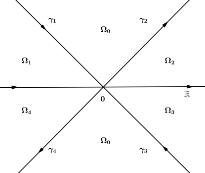
3.2 The RH problem deformations

The triangular factorizations (3.11) suggest deforming the contour for the Riemann-Hilbert problem to a cross centered at $k=-\xi$ (see Figure 3), so that the (transformed) jump matrix converges (as $t\to\infty$) to the identity matrix exponentially fast away from a neighborhood of $k=-\xi$. In general, in order to be able to do this, we have to use analytic approximations of the reflection coefficients $r_{j}(k)$, $j=1,2$ outside the real axis. In order to avoid technical complications related to such approximations and to keep transparent the realization of the main ideas of the asymptotic analysis, we assume in what follows that $r_{j}(k)$, $j=1,2$ are analytic at least in a band containing the real axis. This assumption holds, for example, if the initial value $q_{0}(x)$ is a local (with a finite support) perturbation of the background step function.

Adopting the notations $\hat{\Omega}_{j}$, $j=0,\dots,4$ for the sectors as in Figure 3 (notice that the points $\{p_{j}\}_{1}^{n}$ and $\{-\bar{p}_{j}\}_{1}^{n}$ are located in $\hat{\Omega}_{0}$), we define $\hat{M}(x,t,k)$ as follows:

Refer to caption
Figure 3: The domains $\hat{\Omega}_{j}$, $j=0,\dots,4$ and the contour $\hat{\Gamma}=\hat{\gamma}_{1}\cup...\cup\hat{\gamma}_{4}$
$$\hat{M}(x,t,k)=\begin{cases}\tilde{M}(x,t,k),&k\in\hat{\Omega}_{0},\\ \tilde{M}(x,t,k)\begin{pmatrix}1&\frac{r_{2}(k)\delta^{2}(k,\xi)}{1-r_{1}(k)r_{2}(k)}e^{-2it\theta}\\ 0&1\\ \end{pmatrix},&k\in\hat{\Omega}_{1},\\ \tilde{M}(x,t,k)\begin{pmatrix}1&0\\ -r_{1}(k)\delta^{-2}(k,\xi)e^{2it\theta}&1\\ \end{pmatrix},&k\in\hat{\Omega}_{2},\\ \tilde{M}(x,t,k)\begin{pmatrix}1&-r_{2}(k)\delta^{2}(k,\xi)e^{-2it\theta}\\ 0&1\\ \end{pmatrix},&k\in\hat{\Omega}_{3},\\ \tilde{M}(x,t,k)\begin{pmatrix}1&0\\ \frac{r_{1}(k)\delta^{-2}(k,\xi)}{1-r_{1}(k)r_{2}(k)}e^{2it\theta}&1\\ \end{pmatrix},&k\in\hat{\Omega}_{4}.\end{cases}$$ (3.15)

Then $\hat{M}(x,t,k)$ satisfies the jump (across $\hat{\Gamma}$) and norming

$\displaystyle\hat{M}_{+}(x,t,k)=\hat{M}_{-}(x,t,k)\hat{J}(x,t,k),$ $\displaystyle k\in\hat{\Gamma},$ (3.16a)
$\displaystyle\hat{M}(x,t,k)\rightarrow I,$ $\displaystyle k\rightarrow\infty,$ (3.16b)

with the jump matrix

$$\hat{J}(x,t,k)=\begin{cases}\begin{pmatrix}1&\frac{-r_{2}(k)\delta^{2}(k,\xi)}{1-r_{1}(k)r_{2}(k)}e^{-2it\theta}\\ 0&1\\ \end{pmatrix},&k\in\hat{\gamma}_{1},\\ \begin{pmatrix}1&0\\ r_{1}(k)\delta^{-2}(k,\xi)e^{2it\theta}&1\\ \end{pmatrix},&k\in\hat{\gamma}_{2},\\ \begin{pmatrix}1&r_{2}(k)\delta^{2}(k,\xi)e^{-2it\theta}\\ 0&1\\ \end{pmatrix},&k\in\hat{\gamma}_{3},\\ \begin{pmatrix}1&0\\ \frac{-r_{1}(k)\delta^{-2}(k,\xi)}{1-r_{1}(k)r_{2}(k)}e^{2it\theta}&1\\ \end{pmatrix},&k\in\hat{\gamma}_{4},\end{cases}$$ (3.17)

the residue conditions

$\displaystyle\underset{k=p_{j}}{\operatorname{Res}}\hat{M}^{(1)}(x,t,k)=f_{j}(x,t)\hat{M}^{(2)}(x,t,p_{j}),\quad j=\overline{1,n},$ (3.18a)
$\displaystyle\underset{k=-\overline{p}_{j}}{\operatorname{Res}}\hat{M}^{(1)}(x,t,k)=\tilde{f}_{j}(x,t)\hat{M}^{(2)}(x,t,-\overline{p}_{j}),\quad j=\overline{1,n},$ (3.18b)

with

$$f_{j}(x,t)=\frac{\eta_{j}e^{2ip_{j}x+4ip_{j}^{2}t}}{\dot{a}_{1}(p_{j})\delta^{2}(p_{j},\xi)},\quad\tilde{f}_{j}(x,t)=\frac{e^{-2i\overline{p}_{j}x+4i\overline{p}_{j}^{2}t}}{\bar{\eta}_{j}\dot{a}_{1}(-\overline{p}_{j})\delta^{2}(-\overline{p}_{j},\xi)},$$ (3.19)

the residue condition at $k=0$:

$$\underset{k=0}{\operatorname{Res}}\hat{M}^{(2)}(x,t,k)=c_{0}(\xi)\hat{M}^{(1)}(x,t,0),$$ (3.20)

with $c_{0}(\xi)=\frac{A\delta^{2}(0,\xi)}{2i}$, and the (singular) behavior at $k=-\xi$:

$$\hat{M}(x,t,k)=\left(\hat{M}_{-\xi}(x,t)+O(k+\xi)\right)(k+\xi)^{\mathop{\rm Im}\nolimits\nu(-\xi)\sigma_{3}},\quad k\to-\xi,$$ (3.21)

where $\hat{M}_{-\xi}(x,t)$ is some matrix function with $\det\hat{M}_{-\xi}(x,t)=1$ for all $x$ and $t$.

Notice that the pseudo-residue conditions (2.40) have transformed into (3.20), the latter having the form of a conventional residue condition.

Proposition 4.

For any fixed $\xi=\frac{x}{4t}$, $\xi>0$ such that $\xi\not\in\{\omega_{m}\}_{1}^{n-1}\cup\{\mathop{\rm Re}\nolimits p_{m}\}_{1}^{n}\cup\{0\}$, the solution of the Riemann-Hilbert problem (3.16)-(3.21) can be approximated (as $t\to\infty$) by the solution of a RH problem (denoted by $M^{as}$) characterized by a single residue condition (at $k=0$) and a weak singularity at $k=-\xi$:

$\displaystyle q(x,t)=2i\lim_{k\to\infty}kM_{12}^{as}(\xi,t,k)+O(e^{-Ct}),\quad t\to\infty,$ (3.22)
$\displaystyle q(-x,t)=-2i\lim_{k\to\infty}k\overline{M_{21}^{as}(\xi,t,k)}+O(e^{-Ct}),\quad t\to\infty,$ (3.23)

with some $C>0$. Depending on the value of $\xi$, the approximating RH problem has one of two forms (to make the presentation more compact, we adopt the convention $\prod\limits_{s=m_{1}}^{m_{2}}(\cdot)_{s}=1$, if $m_{1}>m_{2}$):

  1. (i)

    for $-\omega_{n-m}<-\xi<\mathop{\rm Re}\nolimits p_{n-m}$, $m=\overline{0,n-1}$, $M^{as}$ solves the RH problem

    $\displaystyle M^{as}_{+}(\xi,t,k)=M^{as}_{-}(\xi,t,k)J^{as}(\xi,t,k),$ $\displaystyle k\in\hat{\Gamma},$ (3.24a)
    $\displaystyle M^{as}(\xi,t,k)\to I,$ $\displaystyle k\to\infty,$ (3.24b)
    $\displaystyle\underset{k=0}{\operatorname{Res}}M^{as\,(2)}(\xi,t,k)=c_{0}^{as}(\xi)M^{as\,(1)}(\xi,t,0),$ (3.24c)
    $\displaystyle M^{as}(\xi,t,k)=\left(M^{as}_{-\xi}(\xi,t)+O(k+\xi)\right)(k+\xi)^{(\mathop{\rm Im}\nolimits\nu(-\xi)-m)\sigma_{3}},$ $\displaystyle k\to-\xi,$ (3.24d)

    where

    $$c_{0}^{as}(\xi)=\frac{A\delta^{2}(0,\xi)}{2i}\prod\limits_{s=0}^{m-1}\left(\frac{\xi}{p_{n-s}}\right)^{2}$$ (3.25)

    and

    $$J^{as}(\xi,t,k)=\left(\prod\limits_{s=0}^{m-1}\frac{k+\xi}{k-p_{n-s}}\right)^{\sigma_{3}}\hat{J}(x,t,k)\left(\prod\limits_{s=0}^{m-1}\frac{k+\xi}{k-p_{n-s}}\right)^{-\sigma_{3}},\,k\in\hat{\Gamma}.$$ (3.26)
  2. (ii)

    for $\mathop{\rm Re}\nolimits p_{n-m}<-\xi<-\omega_{n-m-1}$, $m=\overline{0,n-1}$, $M^{as}$ solves the RH problem

    $\displaystyle M^{as}_{+}(\xi,t,k)=M^{as}_{-}(\xi,t,k)J^{as}(\xi,t,k),$ $\displaystyle k\in\hat{\Gamma},$ (3.27a)
    $\displaystyle M^{as}(\xi,t,k)\to I,$ $\displaystyle k\to\infty,$ (3.27b)
    $\displaystyle\underset{k=0}{\operatorname{Res}}\ M^{as\,(1)}(\xi,t,k)=c_{0}^{as\#}(\xi)M^{as\,(2)}(\xi,t,0),$ (3.27c)
    $\displaystyle M^{as}(x,t,k)=\left(M^{as}_{-\xi}(x,t)+O(k+\xi)\right)(k+\xi)^{(\mathop{\rm Im}\nolimits\nu(-\xi)-m)\sigma_{3}},$ $\displaystyle k\to-\xi,$ (3.27d)

    where

    $$c_{0}^{as\#}(\xi)=\frac{2ip_{n-m}^{2}}{A\delta^{2}(0,\xi)}\prod\limits_{s=0}^{m-1}\left(\frac{p_{n-s}}{\xi}\right)^{2}$$ (3.28)

    and

    $$J^{as}(\xi,t,k)=\left(d(k)\prod\limits_{s=0}^{m-1}\frac{k+\xi}{k-p_{n-s}}\right)^{\sigma_{3}}\hat{J}(x,t,k)\left(d(k)\prod\limits_{s=0}^{m-1}\frac{k+\xi}{k-p_{n-s}}\right)^{-\sigma_{3}},\,k\in\hat{\Gamma},$$ (3.29)

    with $d(k)=\frac{k}{k-p_{n-m}}$.

Proof.

(i) Consider $\xi$ such that $-\omega_{n-m}<-\xi<\mathop{\rm Re}\nolimits p_{n-m}$, $m=\overline{0,n-1}$. In this case, the RH problem for $\hat{M}(x,t,k)$ involves $m$ residue conditions, at $k=p_{n-s}$, $s=\overline{0,m-1}$, with exponentially growing factors, the other having exponentially decaying factors, see (3.18a). Then, introducing $\check{M}(x,t,k)$ by

$$\check{M}(x,t,k):=\hat{M}(x,t,k)\left(\prod\limits_{s=0}^{m-1}\frac{k+\xi}{k-p_{n-s}}\right)^{-\sigma_{3}},\quad k\in\mathbb{C},$$ (3.30)

we have (see (3.24c)) that $\check{M}(x,t,k)$ satisfies a RH problem with all residue conditions but one (at $k=0$) having exponentially decaying factors. Moreover, $\check{M}(x,t,k)$ satisfies the jump condition with the jump matrix given by (3.26) and has a weak singularity of type (3.24d) (in view of (3.8), $\mathop{\rm Im}\nolimits\nu(-\xi)-m\in(-\frac{1}{2},\frac{1}{2})$). Ignoring the residue conditions with decaying factors, we arrive at the RH problem (3.24).

(ii) Now consider $\mathop{\rm Re}\nolimits p_{n-m}<-\xi<-\omega_{n-m-1}$, $m=\overline{0,n-1}$. In this case, the RH problem for $\hat{M}(x,t,k)$ involves $m+1$ residue conditions, at $k=p_{n-s}$, $s=\overline{0,m}$, with exponentially growing factors. Applying the transformation (3.30) and ignoring the exponentially decaying residue conditions, we arrive at the RH problem with two residue conditions, one of them having an exponentially growing factor: $k=p_{n-m}$ (see (3.19)):

$\displaystyle\tilde{M}^{as}_{+}(\xi,t,k)=\tilde{M}^{as}_{-}(\xi,t,k)\tilde{J}^{as}(\xi,t,k),$ $\displaystyle k\in\hat{\Gamma},$ (3.31a)
$\displaystyle\tilde{M}^{as}(\xi,t,k)\to I,$ $\displaystyle k\to\infty,$ (3.31b)
$\displaystyle\underset{k=p_{n-m}}{\operatorname{Res}}\tilde{M}^{as\,(1)}(\xi,t,k)=f(x,t)\tilde{M}^{as\,(2)}(\xi,t,p_{n-m}),$ (3.31c)
$\displaystyle\underset{k=0}{\operatorname{Res}}\tilde{M}^{as\,(2)}(\xi,t,k)=c_{0}^{as}(\xi)\tilde{M}^{as\,(1)}(\xi,t,0),$ (3.31d)
$\displaystyle\tilde{M}^{as}(x,t,k)=\left(\tilde{M}^{as}_{-\xi}(x,t)+O(k+\xi)\right)(k+\xi)^{(\mathop{\rm Im}\nolimits\nu(-\xi)-m)\sigma_{3}},\,k\to-\xi,$ (3.31e)

where $f(x,t)=f_{n-m}(x,t)\prod\limits_{s=0}^{m-1}\left(\frac{p_{n-m}-p_{n-s}}{p_{n-m}+\xi}\right)^{2}$, $c_{0}^{as}(\xi)$ is given by (3.25), and

$$\tilde{J}^{as}(\xi,t,k)=\left(\prod\limits_{s=0}^{m-1}\frac{k+\xi}{k-p_{n-s}}\right)^{\sigma_{3}}\hat{J}(x,t,k)\left(\prod\limits_{s=0}^{m-1}\frac{k+\xi}{k-p_{n-s}}\right)^{-\sigma_{3}},\,k\in\hat{\Gamma}.$$

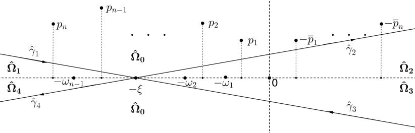
The latter problem has two residue conditions for the different columns, where one of them is exponentially growing and the other one is bounded. Problems of this type can be transformed (see e.g. [17, 46]) in such a way that the exponentially growing conditions ((3.31c), in our case) transform to exponentially decaying. Indeed, the problem (3.31) with residue conditions can be transformed into a regular problem (for $\hat{M}^{as}$) having additional parts of the contour in the form of small circles, $S_{0}$ and $S_{p_{n-m}}$, surrounding respectively $k=0$ and $k=p_{n-m}$, and the enhanced jump conditions:

$\displaystyle\hat{M}^{as}_{+}(x,t,k)=\hat{M}^{as}_{-}(x,t,k)\hat{J}^{as}(x,t,k),$ $\displaystyle k\in\hat{\Gamma}\cup S_{0}\cup S_{p_{n-m}},$ (3.32a)
$\displaystyle\hat{M}^{as}(x,t,k)\to I,$ $\displaystyle k\to\infty,$ (3.32b)

where

$$\hat{J}^{as}(x,t,k)=\begin{cases}\tilde{J}^{as}(x,t,k),&k\in\hat{\Gamma},\\ \begin{pmatrix}1&-\frac{c_{0}^{as}(\xi)}{k}\\ 0&1\end{pmatrix},&k\in S_{0},\\ \begin{pmatrix}1&0\\ -\frac{f(x,t)}{k-p_{n-m}}&1\end{pmatrix},&k\in S_{p_{n-m}}.\end{cases}$$ (3.33)

Next, introducing $\hat{M}^{as\#}$ by

$$\hat{M}^{as\#}(x,t,k)=\begin{cases}\hat{M}^{as}(x,t,k)N(\xi,k)d^{-\sigma_{3}}(k),&k\mbox{ inside }S_{0},\\ \hat{M}^{as}(x,t,k)Q(x,t,k)d^{-\sigma_{3}}(k),&k\mbox{ inside }S_{p_{n-m}},\\ \hat{M}^{as}(x,t,k)d^{-\sigma_{3}}(k),&\mbox{ otherwise },\end{cases}$$ (3.34)

where $d(k)=\frac{k}{k-p_{n-m}}$, $N(\xi,k)=\begin{pmatrix}0&\frac{c_{0}^{as}(\xi)}{k}\\ -\frac{k}{c_{0}^{as}(\xi)}&1\end{pmatrix}$, and $Q(x,t,k)=\begin{pmatrix}1&-\frac{k-p_{n-m}}{f(x,t)}\\ \frac{f(x,t)}{k-p_{n-m}}&0\end{pmatrix},$ straightforward calculations show that the jump matrices for $\hat{M}^{as\#}$ across $S_{p_{n-m}}$ are exponentially decaying (to the identity matrix), whereas the jump across $\hat{\Gamma}$ takes the form (3.29). ∎

Neglecting the jump conditions in (3.24) and (3.27) (recall that due to the signature table, the jump matrices decay, as $t\to\infty$, to the identity matrix exponentially fast outside any vicinity of $k=-\xi$), the RH problems (3.24) and (3.27) reduce, as $t\to\infty$, to algebraic equations that can be solved explicitly:

Mas(ξ,t,k){(1c0as(ξ)k01)for RH (3.24),(10c0as#(ξ)k1),for RH (3.27),similar-to-or-equalssuperscript𝑀𝑎𝑠𝜉𝑡𝑘casesmatrix1superscriptsubscript𝑐0𝑎𝑠𝜉𝑘01for RH (3.24)matrix10superscriptsubscript𝑐0𝑎𝑠#𝜉𝑘1for RH (3.27)M^{as}(\xi,t,k)\simeq\begin{cases}\begin{pmatrix}1&\frac{c_{0}^{as}(\xi)}{k}\\ 0&1\end{pmatrix}&\mbox{for RH (\ref{RHas1})},\\ \begin{pmatrix}1&0\\ \frac{c_{0}^{as\#}(\xi)}{k}&1\end{pmatrix},&\mbox{for RH (\ref{RHas2})},\end{cases} (3.35)

where $c_{0}^{as}(\xi)$ and $c_{0}^{as\#}(\xi)$ are given by (3.25) and (3.28) respectively. Substituting (3.35) into (3.22) and (3.23), the (rough) asymptotics (1.5) in Theorem 1 follow.

Remark 5.

For the focusing NNLS equation [46], the pure step initial function with $R=0$ (i.e., $q_{0}(x)=q_{0,A}(x)$) satisfies assumptions analogous to Assumptions (a)-(c) and thus this case is covered by the corresponding asymptotic formulas. In contrast with this, for the defocusing NNLS equation, $R=0$ is one of the bifurcation values of $R$, see Remark 1.

In order to rigorously justify the asymptotic formulas (1.5), we adapt the nonlinear steepest descent method [16, 20], which also allows us to make the asymptotics presented in (1.5) more precise.

Theorem 2.

Consider the initial value problem (1.2), (1.3). Assume that (i) the initial value $q_{0}(x)$ converges to its boundary values fast enough, (ii) the associated spectral functions $a_{j}(k)$, $j=1,2$ satisfy Assumptions (a)-(c), and (iii) the spectral functions $r_{j}(k)$, $j=1,2$ can be analytically continued from the real axis into a band along it. Assuming also that the solution $q(x,t)$ of (1.2), (1.3) exists, it has the following long-time asymptotics along the rays $\frac{x}{4t}=\xi$:

(i) for $-\omega_{n-m}<-\xi<\mathop{\rm Re}\nolimits p_{n-m}$, $m=\overline{0,n-1}$, there are three types of asymptotics depending on the value of $\mathop{\rm Im}\nolimits\nu(-\xi)$:

  1. 1)

    if $\mathop{\rm Im}\nolimits\nu(-\xi)\in\left(m-\frac{1}{2},m-\frac{1}{6}\right]$, then

    $$q(x,t)=A\delta^{2}(0,\xi)\prod\limits_{s=0}^{m-1}\left(\frac{\xi}{p_{n-s}}\right)^{2}+t^{-\frac{1}{2}-\mathop{\rm Im}\nolimits\nu(-\xi)+m}\alpha_{1}(\xi)\exp\{-4it\xi^{2}+i\mathop{\rm Re}\nolimits\nu(-\xi)\ln t\}+R_{1}(\xi,t).$$
  2. 2)

    if $\mathop{\rm Im}\nolimits\nu(-\xi)\in\left(m-\frac{1}{6},m+\frac{1}{6}\right)$, then

    $\displaystyle q(x,t)=$ $\displaystyle A\delta^{2}(0,\xi)\prod\limits_{s=0}^{m-1}\left(\frac{\xi}{p_{n-s}}\right)^{2}+t^{-\frac{1}{2}-\mathop{\rm Im}\nolimits\nu(-\xi)+m}\alpha_{1}(\xi)\exp\{-4it\xi^{2}+i\mathop{\rm Re}\nolimits\nu(-\xi)\ln t\}$
    $\displaystyle+t^{-\frac{1}{2}+\mathop{\rm Im}\nolimits\nu(-\xi)-m}\alpha_{2}(\xi)\exp\{4it\xi^{2}-i\mathop{\rm Re}\nolimits\nu(-\xi)\ln t\}+R_{3}(\xi,t).$
  3. 3)

    if $\mathop{\rm Im}\nolimits\nu(-\xi)\in\left[m+\frac{1}{6},m+\frac{1}{2}\right)$, then

    $$q(x,t)=A\delta^{2}(0,\xi)\prod\limits_{s=0}^{m-1}\left(\frac{\xi}{p_{n-s}}\right)^{2}+t^{-\frac{1}{2}+\mathop{\rm Im}\nolimits\nu(-\xi)-m}\alpha_{2}(\xi)\exp\{4it\xi^{2}-i\mathop{\rm Re}\nolimits\nu(-\xi)\ln t\}+R_{2}(\xi,t).$$

(ii) for $-\mathop{\rm Re}\nolimits p_{n-m}<-\xi<\omega_{n-m}$, $m=\overline{0,n-1}$:

$$q(x,t)=t^{-\frac{1}{2}-\mathop{\rm Im}\nolimits\nu(\xi)+m}\alpha_{3}(\xi)\exp\{4it\xi^{2}-i\mathop{\rm Re}\nolimits\nu(\xi)\ln t\}+R_{2}(-\xi,t)$$

(iii) for $\mathop{\rm Re}\nolimits p_{n-m}<-\xi<-\omega_{n-m-1}$, $m=\overline{0,n-1}$:

$$q(x,t)=t^{-\frac{1}{2}+\mathop{\rm Im}\nolimits\nu(-\xi)-m}\alpha_{4}(\xi)\exp\{4it\xi^{2}-i\mathop{\rm Re}\nolimits\nu(-\xi)\ln t\}+R_{2}(\xi,t)$$

(iv) for $\omega_{n-m-1}<-\xi<-\mathop{\rm Re}\nolimits p_{n-m}$, $m=\overline{0,n-1}$, there are three types of asymptotics depending on the value of $\mathop{\rm Im}\nolimits\nu(\xi)$:

  1. 1)

    if $\mathop{\rm Im}\nolimits\nu(\xi)\in\left(m-\frac{1}{2},m-\frac{1}{6}\right]$, then

    $$q(x,t)=\frac{-4\overline{p}_{n-m}^{2}}{A\overline{\delta^{2}}(0,-\xi)}\prod\limits_{s=0}^{m-1}\left(\frac{\overline{p}_{n-s}}{\xi}\right)^{2}+t^{-\frac{1}{2}-\mathop{\rm Im}\nolimits\nu(\xi)+m}\alpha_{5}(\xi)\exp\{4it\xi^{2}-i\mathop{\rm Re}\nolimits\nu(\xi)\ln t\}+R_{1}(-\xi,t),$$
  2. 2)

    if $\mathop{\rm Im}\nolimits\nu(\xi)\in\left(m-\frac{1}{6},m+\frac{1}{6}\right)$, then

    $\displaystyle q(x,t)=$ $\displaystyle\frac{-4\overline{p}_{n-m}^{2}}{A\overline{\delta^{2}}(0,-\xi)}\prod\limits_{s=0}^{m-1}\left(\frac{\overline{p}_{n-s}}{\xi}\right)^{2}+t^{-\frac{1}{2}-\mathop{\rm Im}\nolimits\nu(\xi)+m}\alpha_{5}(\xi)\exp\{4it\xi^{2}-i\mathop{\rm Re}\nolimits\nu(\xi)\ln t\}$
    $\displaystyle+t^{-\frac{1}{2}+\mathop{\rm Im}\nolimits\nu(\xi)-m}\alpha_{6}(\xi)\exp\{-4it\xi^{2}+i\mathop{\rm Re}\nolimits\nu(\xi)\ln t\}+R_{3}(-\xi,t).$
  3. 3)

    if $\mathop{\rm Im}\nolimits\nu(\xi)\in\left[m+\frac{1}{6},m+\frac{1}{2}\right)$, then

    $$q(x,t)=\frac{-4\overline{p}_{n-m}^{2}}{A\overline{\delta^{2}}(0,-\xi)}\prod\limits_{s=0}^{m-1}\left(\frac{\overline{p}_{n-s}}{\xi}\right)^{2}+t^{-\frac{1}{2}+\mathop{\rm Im}\nolimits\nu(\xi)-m}\alpha_{6}(\xi)\exp\{-4it\xi^{2}+i\mathop{\rm Re}\nolimits\nu(\xi)\ln t\}+R_{2}(-\xi,t).$$

Here

$$\delta(k,\xi)=(k+\xi)^{i\nu(-\xi)}e^{\chi(k,\xi)},$$ (3.36)

and

$$\nu(-\xi)=-\frac{1}{2\pi}\ln|1+r_{1}(-\xi)r_{2}(-\xi)|-\frac{i}{2\pi}\int_{-\infty}^{-\xi}\,d\arg(1-r_{1}(\zeta)r_{2}(\zeta)),$$ (3.37)

with

$$\chi(k,\xi)=-\frac{1}{2\pi i}\int_{-\infty}^{-\xi}\ln(k-\zeta)d_{\zeta}(1-r_{1}(\zeta)r_{2}(\zeta)).$$ (3.38)

The modulating functions $\alpha_{j}(\xi)$, $j=\overline{1,6}$ are as follows:

$$\alpha_{1}(\xi)=\frac{\sqrt{\pi}(c_{0}^{as}(\xi))^{2}\prod\limits_{s=0}^{m-1}(\xi+p_{n-s})^{2}}{\xi^{2}r_{2}(-\xi)\Gamma(i\nu(-\xi)+m)}\exp\left\{-\frac{\pi}{2}(\nu(-\xi)-im)+\frac{3\pi i}{4}-2\chi(-\xi,\xi)+3(i\nu(-\xi)+m)\ln 2\right\},$$
$$\alpha_{2}(\xi)=\frac{\sqrt{\pi}\prod\limits_{s=0}^{m-1}(\xi+p_{n-s})^{-2}}{r_{1}(-\xi)\Gamma(-i\nu(-\xi)-m)}\exp\left\{-\frac{\pi}{2}(\nu(-\xi)-im)+\frac{\pi i}{4}+2\chi(-\xi,\xi)-3(i\nu(-\xi)+m)\ln 2\right\},$$
$$\alpha_{3}(\xi)=\frac{\sqrt{\pi}\prod\limits_{s=0}^{m-1}(\overline{p}_{n-s}-\xi)^{2}}{\overline{r_{2}}(\xi)\Gamma(-i\overline{\nu(\xi)}+m)}\exp\left\{-\frac{\pi}{2}(\overline{\nu(\xi)}+im)+\frac{\pi i}{4}-2\overline{\chi(\xi,\xi)}-3(i\overline{\nu(\xi)}-m)\ln 2\right\},$$
$$\alpha_{4}(\xi)=\frac{\sqrt{\pi}\xi^{2}\prod\limits_{s=0}^{m}(\xi+p_{n-s})^{-2}}{r_{1}(-\xi)\Gamma(-i\nu(-\xi)-m)}\exp\left\{-\frac{\pi}{2}(\nu(-\xi)-im)+\frac{\pi i}{4}+2\chi(-\xi,\xi)-3(i\nu(-\xi)+m)\ln 2\right\},$$
$$\alpha_{5}(\xi)=\frac{\sqrt{\pi}\prod\limits_{s=0}^{m}(\overline{p}_{n-s}-\xi)^{2}}{\xi^{2}\overline{r_{2}}(\xi)\Gamma(-i\overline{\nu(\xi)}+m)}\exp\left\{-\frac{\pi}{2}(\overline{\nu(\xi)}+im)+\frac{\pi i}{4}-2\overline{\chi(\xi,\xi)}-3(i\overline{\nu(\xi)}-m)\ln 2\right\},$$
$$\alpha_{6}(\xi)=\frac{\sqrt{\pi}\left(\overline{c_{0}^{as\#}(-\xi)}\right)^{2}\prod\limits_{s=0}^{m}(\overline{p}_{n-s}-\xi)^{-2}}{\overline{r_{1}}(\xi)\Gamma(i\overline{\nu(\xi)}-m)}\exp\left\{-\frac{\pi}{2}(\overline{\nu(\xi)}+im)+\frac{3\pi i}{4}+2\overline{\chi(\xi,\xi)}+3(i\overline{\nu(\xi)}-m)\ln 2\right\},$$

where

$$c_{0}^{as}(\xi)=\frac{A\delta^{2}(0,\xi)}{2i}\prod\limits_{s=0}^{m-1}\left(\frac{\xi}{p_{n-s}}\right)^{2},\quad c_{0}^{as\#}(\xi)=\frac{2ip_{n-m}^{2}}{A\delta^{2}(0,\xi)}\prod\limits_{s=0}^{m-1}\left(\frac{p_{n-s}}{\xi}\right)^{2}.$$

Finally, the remainders $R_{j}(\xi,t)$, $j=\overline{1,3}$ are estimated as follows:

$$R_{1}(\xi,t)=\begin{cases}O\left(t^{-1}\right),&\mathop{\rm Im}\nolimits\nu(-\xi)>m,\\ O\left(t^{-1}\ln t\right),&\mathop{\rm Im}\nolimits\nu(-\xi)=m,\\ O\left(t^{-1+2|\mathop{\rm Im}\nolimits\nu(-\xi)-m|}\right),&\mathop{\rm Im}\nolimits\nu(-\xi)<m,\end{cases}$$ (3.39)
$$R_{2}(\xi,t)=\begin{cases}O\left(t^{-1+2|\mathop{\rm Im}\nolimits\nu(-\xi)-m|}\right),&\mathop{\rm Im}\nolimits\nu(-\xi)>m,\\ O\left(t^{-1}\ln t\right),&\mathop{\rm Im}\nolimits\nu(-\xi)=m,\\ O\left(t^{-1}\right),&\mathop{\rm Im}\nolimits\nu(-\xi)<m,\end{cases}$$ (3.40)

and

$$R_{3}(\xi,t)=R_{1}(\xi,t)+R_{2}(\xi,t)=\begin{cases}O\left(t^{-1+2|\mathop{\rm Im}\nolimits\nu(-\xi)-m|}\right),&\mathop{\rm Im}\nolimits\nu(-\xi)\not=m,\\ O\left(t^{-1}\ln t\right),&\mathop{\rm Im}\nolimits\nu(-\xi)=m.\end{cases}$$
Proof.

The implementation of the nonlinear steepest descent method to the Riemann-Hilbert problems (3.24) and (3.27) is similar, in many aspects, to that in the case of the focusing NNLS [46]. Therefore, in what follows we discuss the peculiarities of realization of the method only and refer the reader to [46] for details.

We begin with the analysis of the Riemann-Hilbert problem (3.24) (the analysis of (3.27) is similar). First, we make the following transformation:

$$\check{M}^{as}(x,t,k)=\begin{cases}M^{as}(x,t,k)\begin{pmatrix}1&-\frac{c_{0}^{as}}{k}\\ 0&1\\ \end{pmatrix},&k\mbox{ inside }S_{0},\\ M^{as}(x,t,k),&\mbox{ otherwise},\end{cases}$$

where $S_{0}=\{k:|k|<\varepsilon\}$ with $\varepsilon>0$ small enough. Then $\check{M}^{as}(x,t,k)$ solves the Riemann-Hilbert problem without residue condition:

$\displaystyle\check{M}^{as}_{+}(x,t,k)=\check{M}^{as}_{-}(x,t,k)\check{J}^{as}(x,t,k),$ $\displaystyle k\in\hat{\Gamma}\cup S_{0},$ (3.41a)
$\displaystyle\check{M}^{as}(x,t,k)\to I,$ $\displaystyle k\to\infty,$ (3.41b)

with

$$\check{J}^{as}(x,t,k)=\begin{cases}J^{as}(x,t,k),&k\in\hat{\Gamma},\\ \begin{pmatrix}1&-\frac{c_{0}^{as}}{k}\\ 0&1\end{pmatrix},&k\in S_{0}.\end{cases}$$ (3.42)

Taking into account (3.5), the jump matrix $\check{J}^{as}$ on $\hat{\Gamma}$ can be written as follows:

$$\hat{J}(x,t,k)=\begin{cases}\begin{pmatrix}1&\frac{-\check{r}^{as}_{2}(k)(k+\xi)^{2i\check{\nu}(-\xi)}}{1-\check{r}^{as}_{1}(k)\check{r}^{as}_{2}(k)}e^{-2it\theta+2\chi(k,\xi)}\\ 0&1\\ \end{pmatrix},&k\in\hat{\gamma}_{1},\\ \begin{pmatrix}1&0\\ \check{r}^{as}_{1}(k)(k+\xi)^{-2i\check{\nu}(-\xi)}e^{2it\theta-2\chi(k,\xi)}&1\\ \end{pmatrix},&k\in\hat{\gamma}_{2},\\ \begin{pmatrix}1&\check{r}^{as}_{2}(k)(k+\xi)^{2i\check{\nu}(-\xi)}e^{-2it\theta+2\chi(k,\xi)}\\ 0&1\\ \end{pmatrix},&k\in\hat{\gamma}_{3},\\ \begin{pmatrix}1&0\\ \frac{-\check{r}^{as}_{1}(k)(k+\xi)^{-2i\check{\nu}(-\xi)}}{1-r^{as}_{1}(k)r^{as}_{2}(k)}e^{2it\theta-2\chi(k,\xi)}&1\\ \end{pmatrix},&k\in\hat{\gamma}_{4},\end{cases}$$ (3.43)

where

$\displaystyle\check{r}_{1}^{as}(k)=r_{1}(k)\prod\limits_{s=0}^{m-1}(k-p_{n-s})^{2},$ (3.44a)
$\displaystyle\check{r}_{2}^{as}(k)=r_{2}(k)\prod\limits_{s=0}^{m-1}(k-p_{n-s})^{-2},$ (3.44b)
$\displaystyle i\check{\nu}(-\xi)=i\nu(-\xi)+m.$ (3.44c)

Now we introduce the local parametrix $\check{m}^{as}_{0}(x,t,k)$ using arguments similar to those in the case of the local nonlinear Schrödinger equation (see e.g. [16, 25, 32, 37]):

$$\check{m}^{as}_{0}(x,t,k)=\Delta(\xi,t)m^{\Gamma}(\xi,z(k))\Delta^{-1}(\xi,t),$$ (3.45)

where $z(k)$ is the rescaled variable defined by

$$k=\frac{z}{\sqrt{8t}}-\xi,$$ (3.46)
$$\Delta(\xi,t)=e^{(2it\xi^{2}+\chi(-\xi,\xi))\sigma_{3}}(8t)^{\frac{-i\check{\nu}(-\xi)}{2}\sigma_{3}},$$ (3.47)

$m^{\Gamma}(\xi,z)$ is determined by

$$m^{\Gamma}(\xi,z)=m_{0}(\xi,z)D^{-1}_{j}(\xi,z),\qquad z\in\Omega_{j},\,\,j=\overline{0,4},$$ (3.48)

see Figure 4, where

$$D_{0}(\xi,z)=e^{-i\frac{z^{2}}{4}\sigma_{3}}z^{i\check{\nu}(-\xi)\sigma_{3}},$$
$$\begin{matrix}D_{1}(\xi,z)=D_{0}(\xi,z)\begin{pmatrix}1&\frac{\check{r}^{as}_{2}(-\xi)}{1+\check{r}^{as}_{1}(-\xi)\check{r}^{as}_{2}(-\xi)}\\ 0&1\\ \end{pmatrix},&&D_{2}(\xi,z)=D_{0}(\xi,z)\begin{pmatrix}1&0\\ \check{r}^{as}_{1}(-\xi)&1\\ \end{pmatrix},\\ D_{3}(\xi,z)=D_{0}(\xi,z)\begin{pmatrix}1&-\check{r}^{as}_{2}(-\xi)\\ 0&1\\ \end{pmatrix},&&D_{4}(\xi,z)=D_{0}(\xi,z)\begin{pmatrix}1&0\\ \frac{-\check{r}^{as}_{1}(-\xi)}{1+\check{r}^{as}_{1}(-\xi)\check{r}^{as}_{2}(-\xi)}&1\\ \end{pmatrix},\end{matrix}$$

and $m_{0}(\xi,z)$ is the solution of the following RH problem with a constant jump matrix:

$\displaystyle m_{0+}(\xi,z)=m_{0-}(\xi,z)j_{0}(\xi),$ $\displaystyle z\in\mathbb{R},$ (3.49a)
$\displaystyle m_{0}(\xi,z)=\left(I+O(1/z)\right)e^{-i\frac{z^{2}}{4}\sigma_{3}}z^{i\check{\nu}(-\xi)\sigma_{3}},$ $\displaystyle z\rightarrow\infty,$ (3.49b)

where

$$j_{0}(\xi)=\begin{pmatrix}1+\check{r}^{as}_{1}(-\xi)\check{r}^{as}_{2}(-\xi)&\check{r}^{as}_{2}(-\xi)\\ \check{r}^{as}_{1}(-\xi)&1\end{pmatrix}.$$ (3.50)
Refer to caption
Figure 4: Contour and domains for $m^{\Gamma}(\xi,z)$ in the $z$-plane

The latter problem can be solved explicitly in terms of the parabolic cylinder functions [32]. For obtaining the long time asymptotics of $q(x,t)$ we need the large-$z$ asymptotics of $m^{\Gamma}(\xi,z)$:

$$m^{\Gamma}(\xi,z)=I+\frac{i}{z}\begin{pmatrix}0&\beta(\xi)\\ -\gamma(\xi)&0\end{pmatrix}+O(z^{-2}),\qquad z\to\infty,$$

where

$\displaystyle\beta(\xi)=\dfrac{\sqrt{2\pi}e^{-\frac{\pi}{2}\check{\nu}(-\xi)}e^{-\frac{3\pi i}{4}}}{\check{r}^{as}_{1}(-\xi)\Gamma(-i\check{\nu}(-\xi))},$ (3.51a)
$\displaystyle\gamma(\xi)=\dfrac{\sqrt{2\pi}e^{-\frac{\pi}{2}\check{\nu}(-\xi)}e^{-\frac{\pi i}{4}}}{\check{r}^{as}_{2}(-\xi)\Gamma(i\check{\nu}(-\xi))}.$ (3.51b)

Similarly to [46], we define $\breve{M}^{as}(x,t,k)$ by

$$\breve{M}^{as}(x,t,k)=\begin{cases}\check{M}^{as}(x,t,k)(\check{m}_{0}^{as})^{-1}(x,t,k)V(k),&k\mbox{ inside }S_{-\xi},\\ \check{M}^{as}(x,t,k),&k\mbox{ inside }S_{0},\\ \check{M}^{as}(x,t,k)V(k),&\mbox{ otherwise },\end{cases}$$ (3.52)

where $V(k)=\begin{pmatrix}1&-\frac{c_{0}^{as}}{k}\\ 0&1\end{pmatrix}$ and $S_{-\xi}$ is a small counterclockwise oriented circle centered at $k=-\xi$. Straightforward calculations show that $\breve{M}^{as}$ solves the following RH problem on $\hat{\Gamma}_{1}=\hat{\Gamma}\cup S_{-\xi}$:

$\displaystyle\breve{M}^{as}_{+}(x,t,k)=\breve{M}^{as}_{-}(x,t,k)\breve{J}^{as}(x,t,k),$ $\displaystyle k\in\hat{\Gamma}_{1},$ (3.53)
$\displaystyle\breve{M}^{as}(x,t,k)\to I,$ $\displaystyle k\to\infty,$ (3.54)

with the jump matrix

$$\breve{J}^{as}(x,t,k)=\begin{cases}V^{-1}(k)\check{m}_{0-}^{as}(x,t,k)\check{J}^{as}(x,t,k)(\check{m}_{0+}^{as})^{-1}(x,t,k)V(k),&k\in\hat{\Gamma}_{1},k\mbox{ inside }S_{-\xi},\\ V^{-1}(k)(\check{m}_{0}^{as})^{-1}(x,t,k)V(k),&k\in S_{-\xi},\\ V^{-1}(k)\check{J}^{as}(x,t,k)V(k),&\text{otherwise}.\end{cases}$$ (3.55)

Taking into account (3.52), the solution of the original RH problem is given in terms of $\breve{M}^{as}(x,t,k)$ as follows:

$$q(x,t)=2i\left(c_{0}^{as}+\lim_{k\to\infty}k\breve{M}^{as}_{12}(x,t,k)\right),$$ (3.56)

and

$$q(-x,t)=-2i\lim_{k\to\infty}k\overline{\breve{M}^{as}_{21}(x,t,k)}.$$ (3.57)

For evaluating the large-$t$ asymptotics of $\breve{M}^{as}(x,t,k)$ we need the asymptotics of the local parametrix $(\check{m}_{0}^{as})^{-1}(x,t,k)$:

$$(\check{m}_{0}^{as})^{-1}(x,t,k)=\Delta(\xi,t)(m^{\Gamma})^{-1}(\xi,\sqrt{8t}(k+\xi))\Delta^{-1}(\xi,t)=I+\frac{B(\xi,t)}{\sqrt{8t}(k+\xi)}+\tilde{r}(\xi,t),$$ (3.58)

where the entries of $B(\xi,t)$ are as follows (cf. [46]):

$\displaystyle B_{11}(\xi,t)=B_{22}(\xi,t)=0,$ (3.59a)
$\displaystyle B_{12}(\xi,t)=-i\beta(\xi)e^{4it\xi^{2}+2\chi(-\xi,\xi)}(8t)^{-i\check{\nu}(-\xi)},$ (3.59b)
$\displaystyle B_{21}(\xi,t)=i\gamma(\xi)e^{-4it\xi^{2}-2\chi(-\xi,\xi)}(8t)^{i\check{\nu}(-\xi)},$ (3.59c)

and the remainder is:

$$\tilde{r}(\xi,t)=\begin{pmatrix}O\left(t^{-1-\mathop{\rm Im}\nolimits\check{\nu}(-\xi)}\right)&O\left(t^{-1+\mathop{\rm Im}\nolimits\check{\nu}(-\xi)}\right)\\ O\left(t^{-1-\mathop{\rm Im}\nolimits\check{\nu}(-\xi)}\right)&O\left(t^{-1+\mathop{\rm Im}\nolimits\check{\nu}(-\xi)}\right)\end{pmatrix},\quad t\to\infty.$$ (3.60)

$\breve{M}^{as}(x,t,k)$ can be written as

$$\breve{M}^{as}(x,t,k)=I+\frac{1}{2\pi i}\int\limits_{\hat{\Gamma}_{1}}\mu(x,t,s)(\breve{J}^{as}(x,t,s)-I)\frac{ds}{s-k},$$ (3.61)

where $\mu(x,t,k)$ solves the integral equation

$$\mu(x,t,k)=I+\frac{1}{2\pi i}\lim_{\begin{subarray}{c}k^{\prime}\to k\\ k^{\prime}\in-\mbox{side}\end{subarray}}\int_{\hat{\Gamma}_{1}}\frac{\mu(x,t,s)(\breve{J}^{as}(x,t,s)-I)}{s-k^{\prime}}\,ds.$$ (3.62)

Estimating the rhs of (3.61) (cf. [44]) we conclude that

$\displaystyle\lim_{k\to\infty}k\left(\breve{M}^{as}(x,t,k)-I\right)$ $\displaystyle=-\frac{1}{2\pi i}\int_{S_{-\xi}}V^{-1}(k)((\check{m}_{0}^{as})^{-1}(x,t,k)-I)V(k)\,dk+R(\xi,t)$
$\displaystyle=B^{as}(\xi,t)+R(\xi,t),$ (3.63)

where $R(\xi,t)=\begin{pmatrix}R_{1}(\xi,t)&R_{1}(\xi,t)+R_{2}(\xi,t)\\ R_{1}(\xi,t)&R_{1}(\xi,t)+R_{2}(\xi,t)\end{pmatrix}$ and (see (3.59))

$$B^{as}(\xi,t)=\frac{1}{\sqrt{8t}}\begin{pmatrix}\frac{c_{0}^{as}(\xi)}{\xi}B_{21}(\xi,t)&\frac{(c_{0}^{as}(\xi))^{2}}{\xi^{2}}B_{21}(\xi,t)-B_{12}(\xi,t)\\ -B_{21}(\xi,t)&-\frac{c_{0}^{as}(\xi)}{\xi}B_{21}(\xi,t)\end{pmatrix}.$$ (3.64)

Replacing $\check{r}_{j}^{as}(-\xi)$, $j=1,2$ and $\check{\nu}(-\xi)$ by $r_{j}(-\xi)$, $j=1,2$ and $\nu(-\xi)$ respectively, we arrive at asymptotics described by (i) and (iii).

Returning to the Riemann-Hilbert problem (3.27), the reflection coefficients $\check{r}_{j}^{as}(k)$, $j=1,2$ (see (3.44a) and (3.44b)) have the form

$$r^{as}_{1}(k)=r_{1}(k)d^{-2}(k)\prod\limits_{s=0}^{m-1}\left(k-p_{n-s}\right)^{2},\quad r^{as}_{2}(k)=r_{2}(k)d^{2}(k)\prod\limits_{s=0}^{m-1}\left(k-p_{n-s}\right)^{-2},$$

where $d(k)=\frac{k}{k-p_{n-m}}$. Moreover, $V(k)=\begin{pmatrix}1&0\\ -\frac{c_{0}^{as\#}(\xi)}{k}&1\end{pmatrix}$ in the definition of $\breve{M}^{as}(x,t,k)$ (see (3.52)). Therefore,

$\displaystyle q(x,t)=2i\lim_{k\to\infty}k\breve{M}^{as}_{12}(x,t,k),$ (3.65a)
$\displaystyle q(-x,t)=-2i\left(\overline{c_{0}^{as\#}(\xi)}+\lim_{k\to\infty}k\overline{\breve{M}^{as}_{21}(x,t,k)}\right),$ (3.65b)

and $B^{as}(\xi,t)$ and $R(\xi,t)$ in (3.63) are as follows:

$$B^{as}(\xi,t)=\frac{1}{\sqrt{8t}}\begin{pmatrix}-\frac{c_{0}^{as\#}(\xi)}{\xi}B_{12}(\xi,t)&-B_{12}(\xi,t)\\ \frac{(c_{0}^{as\#}(\xi))^{2}}{\xi^{2}}B_{12}(\xi,t)-B_{21}(\xi,t)&\frac{c_{0}^{as\#}(\xi)}{\xi}B_{12}(\xi,t)\end{pmatrix},$$ (3.66)

and $R(\xi,t)=\begin{pmatrix}R_{1}(\xi,t)+R_{2}(\xi,t)&R_{2}(\xi,t)\\ R_{1}(\xi,t)+R_{2}(\xi,t)&R_{2}(\xi,t)\end{pmatrix}$. Collecting (3.65) and (3.66) we obtain items (ii) and (iv) of the Theorem.

4 Transition regions

In Theorem 2 we present the large-time behavior of the solution $q(x,t)$ along the rays $\xi=\frac{x}{4t}=const$ for all $\xi\not\in\{\pm\mathop{\rm Re}\nolimits p_{m},\pm\omega_{m-1}|m=\overline{1,n}\}$, i.e. for all $\xi\in\mathbb{R}$ except the boundaries of the qualitatively different asymptotic sectors. Since these asymptotic regimes do not match as the slow variable $\xi$ approaches the edges of the sectors, the study of the transition zones between the decaying and constant regimes is a non-trivial task.

We conjecture that there are 3 different types of transition regions in the asymptotics described in Theorem 2:

  1. (1)

    zones near the rays $\xi=\pm\mathop{\rm Re}\nolimits p_{m}$, $m=\overline{1,n}$,

  2. (2)

    zones as $\xi$ approaches to $\omega_{m}$, $m=\overline{1,n-1}$,

  3. (3)

    a zone as $\xi$ approaches to zero.

In the following proposition we describe the transition zones of type (1), where the transition is described by a solitary kink propagating along the rays $\xi=\pm 4\mathop{\rm Re}\nolimits p_{m}$, $m=\overline{1,n}$:

Proposition 5.

Under assumptions of Theorem 2, the solution $q(x,t)$ of problem (1.2), (1.3) has the following asymptotics along the rays $\xi=\pm 4\mathop{\rm Re}\nolimits p_{n-m}$, $m=\overline{0,n-1}$:

$$q(x,t)=\left\{\begin{aligned} &\frac{2ip_{n-m}^{2}c_{0}^{as}(-\mathop{\rm Re}\nolimits p_{n-m})}{p_{n-m}^{2}+c_{0}^{as}(-\mathop{\rm Re}\nolimits p_{n-m})f_{n-m}^{as}(x_{0},t)}+o(1),&t\to\infty,\quad x=-4\mathop{\rm Re}\nolimits p_{n-m}t+x_{0},\\ &\frac{-2i\bar{p}^{2}_{n-m}\overline{f^{as}_{n-m}}(x_{0},t)}{\overline{p}_{n-m}^{2}+\overline{c_{0}^{as}}(-\mathop{\rm Re}\nolimits p_{n-m})\overline{f_{n-m}^{as}}(x_{0},t)}+o(1),&t\to\infty,\quad x=4\mathop{\rm Re}\nolimits p_{n-m}t-x_{0},\\ \end{aligned}\right.$$ (4.1)

where $x_{0}\in\mathbb{R}$, $c_{0}^{as}(\xi)$ is given by (3.25), and $f_{n-m}^{as}(x_{0},t)$ is given by

$$f_{n-m}^{as}(x_{0},t)=\frac{\eta_{n-m}\exp\{2ip_{n-m}x_{0}-4it(\mathop{\rm Re}\nolimits^{2}p_{n-m}+\mathop{\rm Im}\nolimits^{2}p_{n-m})\}}{\dot{a}_{1}(p_{n-m})\delta^{2}(p_{n-m},-\mathop{\rm Re}\nolimits p_{n-m})},\quad m=\overline{0,n-1}.$$ (4.2)

The asymptotics (4.1) is valid for all $t\gg 0$ and $x_{0}\in\mathbb{R}$ such as

$$p_{n-m}^{2}+c_{0}^{as}(-\mathop{\rm Re}\nolimits p_{n-m})f_{n-m}^{as}(x_{0},t)\neq 0.$$

Moreover, as $x_{0}\to\pm\infty$, the asymptotics (4.1) match the asymptotics in the neighboring sectors in (1.5).

Proof.

Similarly to item (i) in Proposition 4, it can be shown that along the rays $\xi=-\mathop{\rm Re}\nolimits p_{n-m}$, $m=\overline{0,n-1}$ (see Figure 3), the long-time behavior of $q(x,t)$ can be described in terns of the solutions of the RH problem (cf. (3.24))

$\displaystyle M^{as}_{+}(\xi,t,k)=M^{as}_{-}(\xi,t,k)J^{as}(\xi,t,k),$ $\displaystyle k\in\hat{\Gamma},$ (4.3a)
$\displaystyle M^{as}(\xi,t,k)\to I,$ $\displaystyle k\to\infty,$ (4.3b)
$\displaystyle\underset{k=0}{\operatorname{Res}}M^{as\,(2)}(\xi,t,k)=c_{0}^{as}(\xi)M^{as\,(1)}(\xi,t,0),$ (4.3c)
$\displaystyle\underset{k=p_{n-m}}{\operatorname{Res}}M^{as\,(1)}(\xi,t,k)=f_{n-m}^{as}(x_{0},t)M^{as\,(2)}(\xi,t,p_{n-m})$ (4.3d)
$\displaystyle M^{as}(\xi,t,k)=\left(M^{as}_{-\xi}(\xi,t)+O(k+\xi)\right)(k+\xi)^{(\mathop{\rm Im}\nolimits\nu(-\xi)-m)\sigma_{3}},$ $\displaystyle k\to-\xi,$ (4.3e)

where $J^{as}(\xi,t,k)$ is given by (3.26) and $x_{0}\in\mathbb{R}$ parametrizes constant parallel shifts of the considered ray: $x=-4\mathop{\rm Re}\nolimits p_{n-m}t-x_{0}$, $m=\overline{0,n-1}$ (notice that such shift does not change the value of the slow variable $\xi=\frac{x}{4t}$ as $t\to\infty$). Using the Blaschke-Potapov factors (see e.g. [24, 45]), the asymptotics of $q(x,t)$ can be found in terms of the solution of a regular Riemann-Hilbert problem:

$\displaystyle q(x,t)$ $\displaystyle=2ip_{n-m}P_{12}(\xi,t)+2i\lim\limits_{k\to\infty}kM^{as,\,R}_{12}(\xi,t,k),\quad x>0,$ (4.4a)
$\displaystyle q(x,t)$ $\displaystyle=-2i\bar{p}_{n-m}\overline{P_{21}(-\xi,t)}-2i\lim\limits_{k\to\infty}k\overline{M^{as,\,R}_{21}(-\xi,t,k)},\quad x<0,$ (4.4b)

where $M^{as,\,R}(\xi,t,k)$ solves the RH problem

$\displaystyle M^{as,\,R}_{+}(\xi,t,k)=M^{as,\,R}_{-}(\xi,t,k)J^{as,\,R}(\xi,t,k),$ $\displaystyle k\in\hat{\Gamma},$ (4.5a)
$\displaystyle M^{as,\,R}(\xi,t,k)\rightarrow I,$ $\displaystyle k\rightarrow\infty,$ (4.5b)
$\displaystyle M^{as,\,R}(\xi,t,k)=\left(M^{as,\,R}_{-\xi}(\xi,t)+O(k+\xi)\right)(k+\xi)^{(\mathop{\rm Im}\nolimits\nu(-\xi)-m)\sigma_{3}},$ $\displaystyle k\to-\xi,$ (4.5c)
with $\xi=-\mathop{\rm Re}\nolimits p_{n-m}$, $m=\overline{0,n-1}$, and
$$J^{as,\,R}(\xi,t,k)=\begin{pmatrix}1&0\\ 0&\frac{k-p_{n-m}}{k}\end{pmatrix}J^{as}(\xi,t,k)\begin{pmatrix}1&0\\ 0&\frac{k}{k-p_{n-m}}\end{pmatrix},\quad k\in\hat{\Gamma}.$$ (4.5d)

Here $P_{12}(\xi,t)$, $P_{21}(\xi,t)$ are determined in terms of $M^{as,\,R}(\xi,t,k)$ as follows:

$$P_{12}(\xi,t)=\frac{g_{1}(\xi,t)h_{1}(\xi,t)}{g_{1}(\xi,t)h_{2}(\xi,t)-g_{2}(\xi,t)h_{1}(\xi,t)},\,P_{21}(\xi,t)=-\frac{g_{2}(\xi,t)h_{2}(\xi,t)}{g_{1}(\xi,t)h_{2}(\xi,t)-g_{2}(\xi,t)h_{1}(\xi,t)},$$ (4.6)

where $g(\xi,t)=\left(\begin{smallmatrix}g_{1}(\xi,t)\\ g_{2}(\xi,t)\end{smallmatrix}\right)$ and $h(\xi,t)=\left(\begin{smallmatrix}h_{1}(\xi,t)\\ h_{2}(\xi,t)\end{smallmatrix}\right)$ are given by

$\displaystyle g(\xi,t)$ $\displaystyle=p_{n-m}M^{as,\,R(1)}(\xi,t,p_{n-m})-f_{n-m}^{as}(x_{0},t)M^{as,\,R(2)}(\xi,t,p_{n-m}),$ (4.7a)
$\displaystyle h(\xi,t)$ $\displaystyle=p_{n-m}M^{as,\,R(2)}(\xi,t,0)+c_{0}^{as}(\xi)M^{as,\,R(1)}(\xi,t,0).$ (4.7b)

Setting $M^{as,R}(\xi,t,k)\approx I$ (as $t\to\infty$), one can calculate $g(\xi,t)$ and $h(\xi,t)$; substituting them into (4.6) and (4.4), the formulas for the main terms in (4.1) follow. ∎

Descriptions of transition zones of type (2) and (3) are open, challenging problems, which are beyond the scope of this paper. For transition zones of type (2), we face the problem of winding of arguments of certain spectral functions, see (2.42), whereas in the case when $\xi$ approaches 0 (the transition zone of type (3)), we encounter another difficulty: the slow variable $\xi$ and the singularity of the Riemann-Hilbert problem (see (2.40) and (3.20)) merge. For the focusing NNLS equation, we partially address the latter problem in [47], for the pure step initial data $q_{0}(x)=q_{0,A}(x)$, where we present a family of different asymptotic zones; particularly, the decaying zones (for $x<0$) are characterized by the decay of order $t^{p}\sqrt{\ln t}$, where $p<0$ parametrizes the family. Applying similar ideas for the defocusing problem seems possible, but it will require substantial modifications since the behavior of the spectral functions as $k\to 0$ in the focusing and defocusing cases is different (see item 5 of Proposition 2).


Concluding remark. In the present work we have considered the Cauchy problem (1.2), (1.3) with the initial data close to the pure step function (1.4) “shifted to the right”, i.e., with $R>0$ (concerning the case $R=0$ see Remark 5). In the case $R<0$ (i.e., for initial data “shifted to the left”), the spectral functions $a_{j}(k)$, $j=1,2$ and $b(k)$ associated with the pure step initial data (1.4) can be explicitly calculated as well, but their analytical properties differ significantly from those in the case with $R>0$, complicating the analysis of location of zeros (particularly, in this case $a_{2}(k)$ is not a constant) and the respective winding properties of the spectral functions. The application of the IST method and subsequent asymptotic analysis in the case $R<0$ remain an open problem.

References

  • [1] M. J. Ablowitz, B.-F. Feng, X.-D. Luo, Z. H. Musslimani, General soliton solution to a nonlocal nonlinear Schrödinger equation with zero and nonzero boundary conditions, Nonlinearity 31 5385 (2018)
  • [2] M. J. Ablowitz, D. J. Kaup, A. C. Newell, and H. Segur, The Inverse Scattering Transform-Fourier Analysis for Nonlinear Problems, Stud. Appl. Math. 53, 249-315 (1974).
  • [3] M. J. Ablowitz, X.-D. Luo and J. Cole, Solitons, the Korteweg-de Vries equation with step boundary values, and pseudo-embedded eigenvalues, J. Math. Phys. 59 091406 (2018).
  • [4] M. J. Ablowitz and Z. H. Musslimani, Integrable nonlocal nonlinear Schrödinger equation, Phys. Rev. Lett. 110 064105 (2013).
  • [5] M. J. Ablowitz and Z. H. Musslimani, Inverse scattering transform for the integrable nonlocal nonlinear Schrödinger equation, Nonlinearity 29 (2016), 915–946.
  • [6] K. Andreiev, I. Egorova, T. L. Lange and G. Teschl, Rarefaction waves of the Korteweg-de Vries equation via nonlinear steepest descent, J. Diff. Eq., 261 (2016) 5371–5410.
  • [7] C. M. Bender and S. Boettcher, Real spectra in non-Hermitian Hamiltonians having P-T symmetry, Phys. Rev. Lett. 80 (1998), 5243.
  • [8] G. Biondini, Riemann problems and dispersive shocks in self-focusing media, Phys. Rev. E, 98 (2018), 052220-7.
  • [9] G. Biondini, E. Fagerstrom, B. Prinari, Inverse scattering transform for the defocusing nonlinear Schrödinger equation with fully asymmetric non-zero boundary conditions, Physica D: Nonlinear Phenomena, 333 (2016), 117–136.
  • [10] G. Biondini, B. Prinari, On the spectrum of the Dirac operator and the existence of discrete eigenvalues for the defocusing nonlinear Schrödinger equation, Stud. Appl. Math. 132, 2 (2014) 138-159.
  • [11] Yu. Bludov, V. Konotop, B. Malomed, Stable dark solitons in PT-symmetric dual-core waveguides, Phys. Rev. A 87 013816 (2013).
  • [12] A. Boutet de Monvel, V. P. Kotlyarov and D. Shepelsky, Focusing NLS Equation: Long-Time Dynamics of Step-Like Initial Data, Int. Math. Res. Not., 7, (2011) 1613-1653
  • [13] D.C. Brody, PT-symmetry, indefinite metric, and nonlinear quantum mechanics, J. Phys. A: Math. Theor. 50 485202 (2017).
  • [14] R. Buckingham and S. Venakides, Long-time asymptotics of the nonlinear Schrödinger equation shock problem, Comm. Pure Appl. Math. 60 (2007), 1349–1414.
  • [15] K. Chen, D.J. Zhang, Solutions of the nonlocal nonlinear Schrödinger hierarchy via reduction, Appl. Math.Lett., 75 (2018) 82-88.
  • [16] P. A. Deift, A. R. Its and X. Zhou, Long-time asymptotics for integrable nonlinear wave equations. In Important developments in Soliton Theory 1980-1990, edited by A. S. Fokas and V. E. Zakharov, New York: Springer, 181–204, 1993.
  • [17] Deift P, S. Kamvissis, T. Kriecherbauer, X. Zhou, The Toda rarefaction problem, Communications on Pure and Applied Mathematics, Vol. XLIX, 35-83, 1996
  • [18] P. A. Deift, S. Venakides, and X. Zhou, The collisionless shock region for the long-time behavior of solutions of the KdV equation, Communications on Pure and Applied Mathematics 47, no. 2 (1994), 199–206.
  • [19] P. A. Deift, S. Venakides, and X. Zhou, New results in small dispersion KdV by an extension of the steepest descent method for Riemann–Hilbert problems, International Mathematics Research Notices, no. 6 (1997), 286–99.
  • [20] P. A. Deift and X. Zhou, A steepest descend method for oscillatory Riemann–Hilbert problems. Asymptotics for the MKdV equation, Ann. Math. 137, no. 2 (1993): 295–368.
  • [21] I. Egorova, Z. Gladka, V. Kotlyarov and G. Teschl, Long-time asymptotics for the Korteweg-de Vries equation with steplike initial data, Nonlinearity, 26 (2013) 1839–1864.
  • [22] I. Egorova, J. Michor and G. Teschl, Rarefaction waves for the Toda equation via nonlinear steepest descent, Discrete Contin. Dyn. Syst. 38, 2007-2028 (2018)
  • [23] G. A. El and M. A. Hoefer, Dispersive shock waves and modulation theory, Physica D: Nonlinear Phenomena, 333 (2016), 11–65.
  • [24] L. D. Faddeev and L. A. Takhtajan, Hamiltonian Methods in the Theory of Solitons. Springer Series in Soviet Mathematics. Springer-Verlag, Berlin, 1987.
  • [25] A. S. Fokas, A.R. Its, A.A. Kapaev and V. Yu. Novokshenov, Painleve Transcendents. The Riemann–Hilbert Approach, AMS, 2006.
  • [26] T. Gadzhimuradov and A. Agalarov, Towards a gauge-equivalent magnetic structure of the nonlocal nonlinear Schrödinger equation, Phys. Rev. A, 93, 062124 (2016).
  • [27] V. S. Gerdjikov and A. Saxena, Complete integrability of nonlocal nonlinear Schrödinger equation, J. Math. Phys. 58 (2017) 013502.
  • [28] A. V. Gurevich, L. P. Pitaevskii, Nonstationary structure of a collisionless shock wave, Zhurnal Eksperimental’noi i Teoreticheskoi Fiziki 65 590-604 (1973).
  • [29] M. Gürses, A. Pekcan, Nonlocal nonlinear Schrödinger equations and their soliton solutions, J. Math. Phys. 59 051501 (2018).
  • [30] R. Jenkins, Regularization of a sharp shock by the defocusing nonlinear Schrödinger equation, Nonlinearity 28 (2015) 2131–2180.
  • [31] E. J. Hruslov, Asymptotics of the solution of the cauchy problem for the Korteweg-de Vries equation with initial data of step type, Math. USSR-Sb. 28, 229–248 (1976).
  • [32] A. R. Its, Asymptotic behavior of the solutions to the nonlinear Schrödinger equation, and isomonodromic deformations of systems of linear differential equations, Doklady Akad. Nauk SSSR 261, no. 1 (1981), 14–18.
  • [33] V. V. Konotop, J. Yang and D. A. Zezyulin, Nonlinear waves in PT-symmetric systems, Rev. Mod. Phys. 88, 035002 (2016).
  • [34] V. P. Kotlyarov and E. Ya. Khruslov, Solitons of the nonlinear Schrödinger equation, which are generated by the continuous spectrum, Teoreticheskaya i Matematicheskaya Fizika 68, no. 2 (1986), 172–86.
  • [35] V.P. Kotlyarov, A.M. Minakov, Riemann–Hilbert problem to the modified Korteveg–deVries equation: Long-time dynamics of the step-like initial data, J. Math. Phys. 51 (2010) 093506.
  • [36] Kotlyarov, V. P., and A. Minakov. “Dispersive shock wave, generalized Laguerre polynomials, and asymptotic solitons of the focusing nonlinear Schrödinger equation.” J. Math. Phys. 60 (2019): 123501.
  • [37] J. Lenells, The nonlinear steepest descent method for Riemann-Hilbert problems of low regularity, Indiana Univ. Math. 66 (2017), 1287–1332.
  • [38] S. Y. Lou, Alice-Bob systems, $\hat{P}-\hat{T}-\hat{C}$ symmetry invariant and symmetry breaking soliton solutions, J. Math. Phys., 59, 083507 (2018).
  • [39] S. Lou and F. Huang, Alice-Bob Physics: Coherent Solutions of Nonlocal KdV Systems, Scientific Reports, 7: 869 (2017)
  • [40] K. T.-R. McLaughlin, P. D. Miller, The $\bar{\partial}$ steepest descent method and the asymptotic behavior of polynomials orthogonal on the unit circle with fixed and exponentially varying nonanalytic weights. Int. Math. Res. Pap. Art. ID 48673, 177 (2006).
  • [41] J. Michor and A. L. Sakhnovich, GBDT and algebro-geometric approaches to explicit solutions and wave functions for nonlocal NLS, J. Phys. A: Math. Theor. 52 025201 (2018).
  • [42] A. Minakov, Asymptotics of step-like solutions for the Camassa–Holm equation, J. Diff. Eq., 261, 11 (2016)
  • [43] M. Onorato, A. R. Osborne, and M. Serio, Modulational instability in crossing sea states: A possible mechanism for the formation of freak waves, Phys. Rev. Lett. 96, 014503 (2006).
  • [44] Ya. Rybalko, D. Shepelsky, Long-time asymptotics for the integrable nonlocal nonlinear Schrödinger equation, J. Math. Phys. 60 031504 (2019).
  • [45] Ya. Rybalko, D. Shepelsky, Long-time asymptotics for the integrable nonlocal nonlinear Schrödinger equation with step-like initial data, Journ. Differential Equations 270 (2021), 694–724. Doi: 10.1016/j.jde.2020.08.003
  • [46] Ya. Rybalko, D. Shepelsky, Long-time asymptotics for the integrable nonlocal focusing nonlinear Schrödinger equation for a family of step-like initial data, arXiv:1908.06415.
  • [47] Ya. Rybalko, D. Shepelsky, Curved wedges in the long-time asymptotics for the integrable nonlocal nonlinear Schrödinger equation, arXiv:2004.05987.
  • [48] T. Valchev, “On a nonlocal nonlinear Schrödinger equation,” In: Slavova, A. (ed) Mathematics in Industry, Cambridge Scholars Publishing, pp. 36–52 (2014).
  • [49] S. Venakides, P. Deift, R. Oba, The Toda shock problem, Comm. Pure Appl. Math. 44 (1991), 1171–1242.
  • [50] A. Sarma, M. Miri, Z. Musslimani, D. Christodoulides, Continuous and discrete Schrödinger systems with parity-time-symmetric nonlinearities, Physical Review E 89 (2014)
  • [51] J. Yang, General N-solitons and their dynamics in several nonlocal nonlinear Schrödinger equations, Physics Letters A 383, 4 (2019), 328–337.
  • [52] B. Yang and J. Yang, General rogue waves in the nonlocal PT-symmetric nonlinear Schrödinger equation, Lett. Math. Phys. 109 (2019), 945–973.
  • [53] V. E. Zakharov and L. A. Ostrovsky, Modulation instability: The beginning, Phys. D 238, 540–548 (2009).
  • [54] Y. Zhang, D. Qiu, Y. Cheng, J. He, Rational Solution of the Nonlocal Nonlinear Schroedinger Equation and Its Application in Optics, Romanian Journal of Physics, 62, 108 (2017).
  • [55] M. Znojil and D.I. Borisov, Two patterns of PT-symmetry break- down in a non-numerical six-state simulation, Ann. Phys., NY 394 40-49, (2018)