Exponential of tridiagonal Toeplitz matrices: applications and generalization

Abstract:

In this paper, an approximate method is presented for computing exponential of tridiagonal Toeplitz matrices. The method is based on approximating elements of the exponential matrix with modified Bessel functions of the first kind in certain values and accordingly the exponential matrix is decomposed as subtraction of a symmetric Toeplitz and a persymmetric Hankel matrix with no need for the matrix multiplication. Also, the matrix is approximated by a band matrix and an error analysis is provided to validate the method. Generalizations for finding exponential of block Toeplitz tridiagonal matrices and some other related matrix functions are derived. Applications of the new idea for solving one and two dimensions heat equations are presented and the stability of resulting schemes is investigated. Numerical illustrations show the efficiency of the new methods.

Keywords: Tridiagonal Toeplitz matrix, Exponential matrix, Modified Bessel functions of the first kind, Heat equation, Toeplitz matrix, Hankel matrix.

1 Introduction

Computation of exponential of a matrix is an important problem because it has widespread applications in science and engineering. Indeed, the matrix exponential is by far the most studied matrix function. The interest in it stems from its key role in the solution of differential equations [4]. More precisely, usually solution of a differential equation at time $t$ is expressed as $\exp(\textbf{A}t)$ to a vector. The precise task and qualitative properties of the solution of a differential equation are important issues that affect the choice of the method for computing the exponential matrix.

There are some ideas for computing exponential of a matrix such as the power series method, Jordan and Schur forms, limit, and Cauchy integral approaches. Some other well-known techniques for computing $\exp(\textbf{A})$ are scaling and squaring scheme, Padé approximation, and interpolation method. In [7] nineteen dubious ways are collected to compute the exponential of a matrix. The scaling and squaring method has become the most widely used because it is the method implemented in MATLAB [1], [4].

Tridiagonal Toeplitz matrices have an important role in various scientific modeling. Some novel properties and applications of the matrices are collected in [10]. These matrices appear in the discretization of the diffusion term and are ill-conditioned. In numerical solution of differential equations, usually a system with the tridiagonal Toeplitz matrix should be solved. Although the system can be solved efficiently, the accuracy and qualitative properties of the resulting solutions are yet challenging issues. Solutions based on the exponential matrix are an alternative idea that is considered e.g. in [3]. In [6] a new splitting method is presented for finding exponential of tridiagonal matrices which appear in the numerical solution of parabolic PDEs. In the present method, we provide an efficient method for computing exponential of tridiagonal Toeplitz matrices. Also, the exponential of the block tridiagonal Toeplitz matrix is considered as application of the new idea for solving the two-dimensional heat equation.

The paper is organized as follows: Section 2 presents some necessary preliminaries which are needed in the next sections. In Section 3, we reduce the problem to computing exponential of a symmetric tridiagonal Toeplitz matrix and the resulting matrix is approximated as subtraction of a symmetric Toeplitz and a persymmetric Hankel matrix with elements that are modified Bessel functions of the first kind in certain values. In continuation, a band approximation of the exponential matrix is presented and its error is analyzed. Section 6 is devoted to the applications of the new approach for solving and analysis of heat equation in one and two dimensional. Section 7 contains numerical examples for illustrating the efficiency of the new methods. Concluding remarks are collected in Section 8.

2 Preliminaries

In this section, some needed concepts which usually are taken from [5] are presented.

Definition 2.1.

An $n\times n$ Toeplitz matrix is a matrix of the form

$$\textbf{T}=\mathrm{Toeplitz}(\textbf{u},\textbf{v})=\begin{bmatrix}a_{0}&a_{-1}&a_{-2}&\dots&a_{-(n-1)}\\ a_{1}&a_{0}&a_{-1}&\dots&a_{-(n-2)}\\ a_{2}&a_{1}&a_{0}&\dots&a_{-(n-3)}\\ \vdots&\vdots&\vdots&\ddots&\vdots\\ a_{n-1}&a_{n-2}&a_{n-3}&\dots&a_{0}\end{bmatrix}.$$

where $\textbf{u}=(a_{0},a_{1},\ldots,a_{n-1})$ and $\textbf{v}=(a_{0},a_{-1},\ldots,a_{-(n-1)})$. in other words for the $i,j-$th element of T, we have $\textbf{T}_{ij}=a_{i-j}$.

Definition 2.2.

An $n\times n$ matrix $\textbf{A}_{n}$ is called tridiagonal Toeplitz matrix if $a_{i-j}=0$ for $|i-j|>1$ and is denoted by $\textbf{A}_{n}=\mathrm{tridiag}(a_{1},a_{0},a_{-1})$.

Throughout this paper, we denote $n\times n$ tridiagonal Toeplitz matrix by $\textbf{A}_{n}=\mathrm{tridiag}(a,b,c)$ and symmetric tridiagonal Toeplitz matrix is denoted by $\textbf{T}_{n}=\mathrm{tridiag}(z,b,z)$.

Theorem 2.3.

The eigenvalues of $\textbf{T}_{n}$ are

$$\lambda_{k}=b+2z\cos\left(\dfrac{k\pi}{n+1}\right),\qquad k=1,\ldots,n,$$

and an eigenvector corresponding to $\lambda_{k}$ is $v^{(k)}=(v_{1}^{(k)},\ldots,v_{n}^{(k)})^{T}$ where

$$v_{j}^{(k)}=\sin\left(\dfrac{j\pi k}{n+1}\right),\qquad j=1,\ldots,n.$$

Definition 2.4.

The exponential of an $n\times n$ matrix A, denoted by $\exp(\textbf{A})$, is the matrix given by the power series

$$\exp(\textbf{A}):=\sum_{k=0}^{\infty}\dfrac{\textbf{A}^{k}}{k!},$$

where $\textbf{A}^{0}=\textbf{I}_{n}$.

Definition 2.5.

An ${n\times n}$ matrix A is called persymmetric if $\textbf{A}_{ij}=\textbf{A}_{n+1-i,n+1-j}$ for all $1\leq i,j\leq n$, or equivalently, if $\textbf{A}=\textbf{J}\textbf{A}^{T}\textbf{J}$ in which J is the backward identity.

Lemma 2.6.

If matrix A is persymmetric then $\exp(\textbf{A})$ is persymmetric.

Proof.

The proof is immediate by definition. ∎

Definition 2.7.

An $n\times n$ persymmetric Hankel matrix is a matrix of the form

$$\textbf{H}=\mathrm{Hankel}(\textbf{u},\textbf{v})=\begin{bmatrix}a_{-(n-1)}&\dots&a_{-2}&a_{-1}&a_{0}\\ a_{-(n-2)}&\dots&a_{-1}&a_{0}&a_{1}\\ a_{-(n-3)}&\dots&a_{0}&a_{1}&a_{2}\\ \vdots&\ddots&\vdots&\vdots&\vdots\\ a_{0}&\dots&a_{n-3}&a_{n-2}&a_{n-1}\end{bmatrix}.$$

$\textbf{u}=(a_{-(n-1)},\ldots,a_{-1},a_{0},)$ and $\textbf{v}=(a_{0},a_{1},\ldots,a_{(n-1)})$. in other words for the $i,j-$th element of H, we have $\textbf{H}_{ij}=a_{(i+j)-(n+1)}$.

Definition 2.8.

An $n\times n$ matrix $\textbf{Z}_{n}$ is called anti-tridiagonal Hankel matrix if $a_{i-j}=0$ for $|i-j|>1$ and is denoted by $\textbf{Z}_{n}=\mathrm{anti-tridiag}(a_{1},a_{0},a_{-1})$.

Let A and C are $n\times n$, B and D are $m\times m$ matrices respectively.

Definition 2.9.

The Kronecker product of A and B is

$$\textbf{A}\otimes\textbf{B}=[a_{ij}\textbf{B}]_{i,j=1}^{n}=\begin{bmatrix}a_{11}\textbf{B}&\ldots&a_{1n}\textbf{B}\\ \vdots&\ddots&\vdots\\ a_{n1}\textbf{B}&\ldots&a_{nn}\textbf{B}\end{bmatrix}.$$

Definition 2.10.

The Kronecker sum of A and B denoted as $\textbf{A}\oplus\textbf{B}$, is defined by

$$\textbf{A}\oplus\textbf{B}=\textbf{A}\otimes\textbf{I}_{m}+\textbf{I}_{n}\otimes\textbf{B}.$$

Also, the following statements are true

• $\textbf{A}\otimes(\lambda\textbf{B})=(\lambda\textbf{A})\otimes\textbf{B}=\lambda(\textbf{A}\otimes\textbf{B}).$

• $\exp(\textbf{A}\oplus\textbf{B})=\exp(\textbf{A})\otimes\exp(\textbf{B}).$

• $(\textbf{A}\otimes\textbf{B})(\textbf{C}\otimes\textbf{D})=(\textbf{A}\textbf{C})\otimes(\textbf{B}\textbf{D}).$

• If $\lambda$ be an eigenvalue of A and $\mu$ be an eigenvalue of B then $\lambda\mu$ is an eigenvalue of $\textbf{A}\otimes\textbf{B}$.

3 Exponential of tridiagonal Toeplitz matrices

In this section by a similarity between $\textbf{A}_{n}$ and $\textbf{T}_{n}$, the problem is reduced to computing exponential of a symmetric tridiagonal Toeplitz matrix.

Theorem 3.1.

For nonzero $a,c$, we have the following similarity for $\textbf{A}_{n}=\mathrm{tridiag}(a,b,c)$

$$\textbf{A}_{n}=\textbf{D}_{n}\textbf{T}_{n}\textbf{D}_{n}^{-1},$$

where $\textbf{D}_{n}=\mathrm{diag}[\rho_{1},\ldots,\rho_{n}]$, $\rho_{k}=\left(\sqrt{\dfrac{a}{c}}\right)^{k-1}$ and $\textbf{T}_{n}=\mathrm{tridiag}\left(c\sqrt{\dfrac{a}{c}},b,c\sqrt{\dfrac{a}{c}}\right)$.

Proof.

The result is straightforward by matrix multiplication. ∎

According to Theorem (3.1), in the rest of the paper we focus on computing exponential of $\textbf{T}_{n}$.

3.1 Diagonalization of $\textbf{T}_{n}$

To determine $\exp(\textbf{T}_{n})$, we first focus on the matrix $\textbf{H}_{n}=\mathrm{tridiag}(z,0,z)$. From Theorem 2.3 for $z\neq 0$ we know that $\textbf{H}_{n}$ has different eigenvalues. Let

$$\textbf{P}_{n}=[\omega^{(1)},\ldots,\omega^{(n)}]$$ (3.1)

where $\omega^{(k)}=\dfrac{v^{(k)}}{\|v^{(k)}\|_{2}}$, $v^{(k)}=\left(\sin\left(\dfrac{\pi k}{n+1}\right),\ldots,\sin\left(\dfrac{n\pi k}{n+1}\right)\right)^{T}$. Then

$$\textbf{H}_{n}\textbf{P}_{n}=\textbf{P}_{n}\textbf{D}_{n},$$ (3.2)

where $\textbf{D}_{n}=\text{diag}[\lambda_{1},\ldots,\lambda_{n}]$, $\lambda_{k}$ is an eigenvalue of $\textbf{H}_{n}$.

Lemma 3.2.

If $\theta\neq 2k\pi$ for $k\in\mathbb{Z}$, then for $n\in\mathbb{N}$ we have

$$\sum_{t=1}^{n}\cos(t\theta)=\dfrac{\sin\left(\dfrac{n\theta}{2}\right)\cos\left(\dfrac{(n+1)\theta}{2}\right)}{\sin\left(\dfrac{\theta}{2}\right)}.$$

Proof.

The proof is immediate by induction. ∎

Lemma 3.3.

Suppose $n\in\mathbb{N}$ and $1\leq i,j\leq n$ then

$$\sum_{t=1}^{n}\sin\left(\dfrac{t\pi i}{n+1}\right)\sin\left(\dfrac{t\pi j}{n+1}\right)=\begin{cases}\dfrac{n+1}{2}&i=j\\ \quad 0&i\neq j\end{cases}$$

Proof.

Let $i=j$ so $\dfrac{j\pi}{n+1}\neq 2k\pi$ for $k\in\mathbb{Z}$. Therefore according to Lemma 3.2 equality is proved. Let $i\neq j$ if $i$ and $j$ are both even or odd numbers then $i+j=2k$ and $i-j=2k^{\prime}$ for $k,k^{\prime}\in\mathbb{Z}$. Therefore according to Lemma 3.2

$$\sum_{t=1}^{n}\sin\left(\dfrac{t\pi i}{n+1}\right)\sin\left(\dfrac{t\pi j}{n+1}\right) =\sum_{t=1}^{n+1}\sin\left(\dfrac{t\pi i}{n+1}\right)\sin\left(\dfrac{t\pi j}{n+1}\right)$$

$$=0.$$

Now if $i$ is an even number and $j$ is an odd number or conversely then $i+j\neq 2k$ and $i-j\neq 2k^{\prime}$ for all $k,k^{\prime}\in\mathbb{Z}$. Then

$$\sum_{t=1}^{n}\sin\left(\dfrac{t\pi i}{n+1}\right)\sin\left(\dfrac{t\pi j}{n+1}\right) =\dfrac{1}{2}\sum_{t=1}^{n}\cos\left(\dfrac{t\pi(i-j)}{n+1}\right)-\dfrac{1}{2}\sum_{t=1}^{n}\cos\left(\dfrac{t\pi(i+j)}{n+1}\right)$$

$$=0.$$

∎

Corollary 3.4.

Suppose $n\in\mathbb{N}$,
1. For all $v^{(k)}$ in Theorem 2.3, $\|v^{(k)}\|^{2}_{2}=\dfrac{n+1}{2}$.
2. For matrix $\textbf{P}_{n}$ in 3.1, $\textbf{P}_{n}^{-1}=\textbf{P}_{n}^{T}$.

Proof.

The proof is immediate from the use of Lemma 3.3. ∎

According to equality in 3.2 and Corollary 3.4 then $\textbf{H}_{n}=\textbf{P}_{n}\textbf{D}_{n}\textbf{P}_{n}^{T}$ so

$$\exp(\textbf{H}_{n})=\textbf{P}_{n}\exp(\textbf{D}_{n})\textbf{P}_{n}^{T},$$

where

$$\exp(\textbf{D}_{n})=\mathrm{diag}[\exp(\lambda_{1}),\ldots,\exp(\lambda_{n})].$$

Let $a_{ij}^{n}$ is the $i,j-$th element of $\exp(\textbf{H}_{n})$ so we have

$$a_{ij}^{n} =\dfrac{2}{n+1}\sum_{k=1}^{n}\exp\left(2z\cos\left(\dfrac{k\pi}{n+1}\right)\right)\sin\left(\dfrac{k\pi i}{n+1}\right)\sin\left(\dfrac{k\pi j}{n+1}\right)$$

$$=\dfrac{1}{n+1}\sum_{k=1}^{n}\exp\left(2z\cos\left(\dfrac{k\pi}{n+1}\right)\right)\cos\left(\dfrac{k\pi(i-j)}{n+1}\right)$$ (3.3)

$$-\dfrac{1}{n+1}\sum_{k=1}^{n}\exp\left(2z\cos\left(\dfrac{k\pi}{n+1}\right)\right)\cos\left(\dfrac{k\pi(i+j)}{n+1}\right).$$

As a result of Lemma 2.6, $\exp(\textbf{H}_{n})$ is persymmetric. It is also symmetric. Therefore, it is sufficient to compute $a^{n}_{ij}$ only when $j\leq i$ and $i+j\leq n+1$.

Computing elements (3.1) is time-consuming and difficult when $n$ is large. The main contribution of this paper is the approximating of elements based on modified Bessel functions of the first kind in a way that avoids the matrix multiplication. In the next parts, asymptotic behavior and computation of elements of $\exp(\textbf{H}_{n})$ are discussed.

3.2 Asymptotic behavior of elements

In this section, we focus on some properties of modified Bessel functions of the first kind [2].

Definition 3.5.

The modified Bessel functions of the first kind denoted by $I_{n}(x)$ for $x\in\mathbb{C}$ and $n\in\mathbb{Z}$ is

$$I_{n}(x)=\sum_{s=0}^{\infty}\dfrac{1}{s!(n+s)!}\left(\dfrac{x}{2}\right)^{n+2s},$$

and the integral form is

$$I_{n}(x)=\dfrac{1}{\pi}\int_{0}^{\pi}\exp(x\cos(\theta))\cos(n\theta)\mathrm{d}\theta.$$

Lemma 3.6.

Suppose $I_{n}(x)$ is modified Bessel function of the first kind. Then

$$\exp(x)=I_{0}(x)+2\sum_{n=1}^{\infty}I_{n}(x)$$

Lemma 3.7.

For $x>0$ and $n>-\dfrac{1}{2}$, the Bessel functions of the first kind $I_{n}(x)$ satisfy the inequality [13]

$$I_{n}(x)<\frac{x^{n}}{2^{n}n!}\exp(x).$$

Clearly for nonzero $x\in\mathbb{C}$ and $n\geq 0$ we have

$$|I_{n}(x)| \leq I_{n}(|x|)$$ (3.4)

$$<\frac{|x|^{n}}{2^{n}n!}\exp(|x|),$$

and thus

$$\lim_{n\rightarrow+\infty}I_{n}(x)=0.$$

Lemma 3.8.

For $x>0$ and $n\geq-\dfrac{1}{2}$, the Bessel functions of the first kind $I_{n}(x)$ satisfy the inequality [9]

$$I_{n+1}(x)<I_{n}(x).$$

By this lemma, for all $x\in\mathbb{C}$, $m,n\in\mathbb{N}$ if $m>n\geq 0$ then

$$|I_{m}(x)|<I_{n}(|x|)$$ (3.5)

From (3.1) we know

$$\lim_{n\rightarrow+\infty}a_{ij}^{n}=I_{i-j}(2z)-I_{i+j}(2z),$$ (3.6)

So we can write

$$\forall\varepsilon>0\qquad\exists N_{0}\in\mathbb{N}\qquad\forall n\geq N_{0}\qquad|a_{ij}^{n}-(I_{i-j}(2z)-I_{i+j}(2z))|<\varepsilon.$$

Now for $z\neq 0$, put $\varepsilon=I_{i-j}(|2z|)>0$. Then there exists $N_{0}\in\mathbb{N}$ for all $n\geq N_{0}$ such that

$$|a_{ij}^{n}-(I_{i-j}(2z)-I_{i+j}(2z))|<I_{i-j}(|2z|),$$

and also there exists $N_{1}\in\mathbb{N}$ such that for all $1\leqslant n<N_{0}$ we have

$$|a_{ij}^{n}-(I_{i-j}(2z)-I_{i+j}(2z))|<N_{1}I_{i-j}(|2z|).$$

Therefore, for all $n\in\mathbb{N}$

$$|a_{ij}^{n}|<N_{1}I_{i-j}(|2z|)+I_{i-j}(|2z|)+I_{i+j}(|2z|),$$

and thus

$$|a_{ij}^{n}|<(N_{1}+2)I_{i-j}(|2z|).$$

Since

$$\lim_{|i-j|\rightarrow+\infty}I_{i-j}(|2z|)=0,$$

we have

$$\lim_{|i-j|\rightarrow+\infty}a_{ij}^{n}=0.$$

This shows that by going away from the diagonal in each row, elements tend to zero. In the next part, a more practical analysis of $|a_{ij}^{n}|$ is provided to obtain an efficient numerical solution.

3.3 Approximation of $\exp(\textbf{T}_{n})$

In this section we find an approximation of $|a_{ij}^{n}|$ and then a method will provide for computing $\exp(\textbf{T}_{n})$.

According to [12], let $v$ be a real or complex $2\pi-$periodic function on the real line, and define

$$\int_{0}^{2\pi}v(\theta)\mathrm{d}\theta.$$

For any positive integer $N$, the trapezoidal rule for approximating the integral now takes the form

$$I_{N}=\frac{2\pi}{N}\sum_{k=1}^{N}v(\theta_{k}),$$

where $\theta_{k}=2\pi k/N$. The following theorem gives a sharp error bound for the trapezoidal rule for approximating integral of $2\pi-$periodic functions [12].

Theorem 3.9.

Suppose $v$ is $2\pi-$periodic and analytic and satisfies $|v(\theta)|\leq M$ in the strip $-s<Im\theta<s$ for some $s>0$. Then for any $N\geq 1$,

$$|I-I_{N}|\leq\frac{4\pi M}{\exp(sN)-1},\\$$

and the constant $4\pi$ is as small as possible.

Now apply Theorem 3.9 for approximating

$$\frac{1}{\pi}\int_{0}^{2\pi}\exp(2z\cos(\theta))\sin(i\theta)\sin(j\theta)\mathrm{d}\theta,$$

with the trapezoidal rule

$$I^{(i,j)}_{n+1}:=\dfrac{2}{2n+2}\sum_{k=1}^{2n+2}\exp\left(2z\cos\left(\dfrac{2k\pi}{2n+2}\right)\right)\sin\left(\dfrac{2k\pi i}{2n+2}\right)\sin\left(\dfrac{2k\pi j}{2n+2}\right).$$

Since $|\cos(\theta)|$ and $|\sin(\theta)|$ have an upper bound in the strip $-s<Im\theta<s$ at $\theta=\pm is$, where its value is $\cosh(s)$, an upper bound for the integrand is

$$\exp(2\operatorname{Re}(z)\cosh(s))\cosh(is)\cosh(js).$$

Let $s=\ln(2n+2)$, thus for sufficiently large values of $n$ we have $\cosh(s)\sim n+1$ and $\cosh(is)\sim(2n+2)^{i}/2$. Thus according to Theorem 3.9

$$\left|\frac{1}{\pi}\int_{0}^{\pi}\exp(2z\cos(\theta))\sin(i\theta)\sin(j\theta)\mathrm{d}\theta-a^{n}_{i,j}\right|$$

$$=\dfrac{1}{2} \left|\frac{1}{\pi}\int_{0}^{2\pi}\exp(2z\cos(\theta))\sin(i\theta)\sin(j\theta)\mathrm{d}\theta-I^{(i,j)}_{n+1}\right|$$

$$\leq\frac{1}{2}\frac{1}{\pi}\frac{4\pi\exp(2\operatorname{Re}(z)(n+1))\frac{(2n+2)^{i+j}}{4}}{(2n+2)^{2n+2}-1}\sim\frac{1}{2}\frac{\exp(2\operatorname{Re}(z)(n+1))(2n+2)^{i+j}}{(2n+2)^{2n+2}}$$

Therefore,

$$\left|\frac{1}{\pi}\int_{0}^{\pi}\exp(2z\cos(\theta))\sin(i\theta)\sin(j\theta)\mathrm{d}\theta-a^{n}_{i,j}\right|\lesssim\frac{1}{2}\frac{(\exp(2\operatorname{Re}(z)))^{n+1}}{(2n+2)^{2n+2-i-j}}.$$ (3.7)

So, $a^{n}_{ij}$ tends geometrically to $I_{i-j}(2z)-I_{i+j}(2z)$. Since $\exp(\textbf{H}_{n})$ is symmetric and persymmetric, we need only to find an approximation of $a^{n}_{ij}$ for $j\leq i$ and $i+j\leq n+1$.

The following theorem provides a decomposition representation of $\exp(\textbf{H}_{n})$.

Theorem 3.10.

The matrix $\exp(\textbf{H}_{n})$ can be approximated geometrically as subtraction of symmetric Toeplitz matrix and a persymmetric Hankel matrix.

Proof.

By (3.7) and (3.6), with a geometrical accuracy we have

$$a^{n}_{ij}\simeq I_{i-j}(2z)-I_{i+j}(2z),$$

thus

$$\exp(\textbf{H}_{n}) \simeq\begin{bmatrix}I_{0}(2z)&I_{1}(2z)&I_{2}(2z)&\dots&I_{n-1}(2z)\\ I_{1}(2z)&I_{0}(2z)&I_{1}(2z)&\dots&I_{n-2}(2z)\\ I_{2}(2z)&I_{1}(2z)&I_{0}(2z)&\dots&I_{n-3}(2z)\\ \vdots&\vdots&\vdots&\ddots&\vdots\\ I_{n-1}(2z)&I_{n-2}(2z)&I_{n-3}(2z)&\ldots&I_{0}(2z)\end{bmatrix}$$

$$-\begin{bmatrix}I_{2}(2z)&I_{3}(2z)&I_{4}(2z)&\ldots&I_{n+1}(2z)\\ I_{3}(2z)&I_{4}(2z)&I_{5}(2z)&\ldots&I_{n}(2z)\\ I_{4}(2z)&I_{5}(2z)&I_{6}(2z)&\ldots&I_{n-1}(2z)\\ \vdots&\vdots&\vdots&\ddots&\vdots\\ I_{n+1}(2z)&\quad I_{n}(2z)&I_{n-1}(2z)&\dots&I_{2}(2z)\end{bmatrix}$$

So

$$\exp(\textbf{H}_{n})\simeq\text{Toeplitz}(\textbf{u},\textbf{u})-\text{Hankel}(\textbf{v},\textbf{v}),$$

where $\textbf{u}=[I_{0}(2z),\ldots,I_{n-1}(2z)]$ and $\textbf{v}=[I_{n+1}(2z),\ldots,I_{2}(2z)]$. ∎

According to

$$\exp(\textbf{T}_{n})=\exp(b)\exp(\textbf{H}_{n}),$$

we have

$$\exp(\textbf{T}_{n})\simeq\textbf{G}_{n},$$ (3.8)

where $\textbf{G}_{n}=\exp(b)(\text{Toeplitz}(\textbf{u},\textbf{u})-\text{Hankel}(\textbf{v},\textbf{v}))$ with elements $g^{n}_{ij}$.

The approximation (3.8) allows us to replace elements of the exponential matrix by only certain values of $n+2$ modified Bessel functions which can be computed with a standard command in a software or with the trapezoidal rule with $m$ quadrature points for $m\ll n$. Thus computational complexity of the method is of order $n$. This fact especially is useful when $n$ is large. In numerical illustrations efficiency of the method is examined.

The next lemma gives accuracy of (3.8).

Lemma 3.11.

For each $n$ we have

$$\|\exp(\textbf{T}_{n})-\textbf{G}_{n}\|_{\infty}\leq\frac{1}{2}\exp(\operatorname{Re}(b))\left(\frac{\exp(2\operatorname{Re}(z))}{2n+2}\right)^{n+1}.$$

Proof.

Set $k=i+j$, by (3.7) we know

$$\|\exp(\textbf{T}_{n})-\textbf{G}_{n}\|_{\infty} \leq\sum_{k=2}^{n+1}\frac{1}{2}\exp(\operatorname{Re}(b))\frac{\exp(2\operatorname{Re}(z)(n+1))}{(2n+2)^{2n+2}}(2n+2)^{k}$$

$$\leq\frac{1}{2}\exp(\operatorname{Re}(b))\frac{\exp(2\operatorname{Re}(z)(n+1))}{(2n+2)^{2n}}\sum_{k=0}^{n-1}(2n+2)^{k}$$

$$=\frac{1}{2}\exp(\operatorname{Re}(b))\frac{\exp(2\operatorname{Re}(z)(n+1))}{(2n+2)^{2n}}\frac{(2n+2)^{n}-1}{2n+1}$$

$$\sim\frac{1}{2}\exp(\operatorname{Re}(b))\frac{\exp(2\operatorname{Re}(z)(n+1))(2n+2)^{n-1}}{(2n+2)^{2n}}$$

$$=\frac{1}{2}\exp(\operatorname{Re}(b))\left(\frac{\exp(2\operatorname{Re}(z))}{2n+2}\right)^{n+1}.$$

∎

According to this lemma, it is clear that value of $z$ has more effect in accuracy of the solution in comparison with value of $b$.

Definition 3.12.

Let A and B be $n\times n$ matrices. The Hadamard product of A and B is defined by $(\textbf{A}\circ\textbf{B})_{ij}=(\textbf{A})_{ij}(\textbf{B})_{ij}$ for all $1\leq i,j\leq n$.

Theorem 3.13.

The matrix $\exp(\textbf{A}_{n})$ can be approximated geometrically as $\textbf{F}_{n}\circ\textbf{G}_{n}$ where $z=c\sqrt{\dfrac{a}{c}}$, $\textbf{F}_{n}=\mathrm{Toeplitz}(\textbf{u},\textbf{v})$, $\textbf{u}=(a_{0},a_{1},\ldots,a_{n-1})$, $\textbf{v}=(a_{0},a_{-1},\ldots,a_{-(n-1)})$ and $a_{i-j}=\left(\sqrt{\dfrac{a}{c}}\right)^{i-j}$.

Proof.

Accroding to (3.8) and Theorem 3.1

$$\exp(\textbf{A}_{n})\simeq\textbf{D}_{n}\textbf{G}_{n}\textbf{D}_{n}^{-1},$$

so $i,j$-th element of $\exp(\textbf{A}_{n})$ is

$$\dfrac{\rho_{i}}{\rho_{j}}(g^{n}_{ij})=\left(\sqrt{\dfrac{a}{c}}\right)^{i-j}(g^{n}_{ij}).$$

Thus $\exp(\textbf{A}_{n})\simeq\textbf{E}_{n}$ where $\textbf{E}_{n}=\textbf{F}_{n}\circ\textbf{G}_{n}$ with elements $e_{ij}^{n}$. ∎

Let $\textbf{E}_{n,d}$ be a band matrix which is resulted from setting $e_{ij}^{n}=0$ for $|i-j|>d$ where $0\leq d\leq n-1$. In the following theorem the error of this approximation is investigated which is important in applications.

Theorem 3.14.

For $0\leq d\leq n-1$ we have

$$\|\textbf{E}_{n}-\textbf{E}_{n,d}\|_{\infty}\leq 2\frac{|z|^{d}\delta^{n}}{d!}\exp(\operatorname{Re}(b)+3|z|).$$

where $\delta:=\max\left\{\left|\sqrt{\dfrac{a}{c}}\right|,\left|\left(\sqrt{\dfrac{a}{c}}\right)^{-1}\right|\right\}$.

Proof.

By (3.5) for each $z\in\mathbb{C}$

$$|I_{i-j}(2z)-I_{i+j}(2z)|\leq 2I_{i-j}(2|z|)$$

thus

$$|e^{n}_{ij}|\leq 2\exp(\operatorname{Re}(b))I_{i-j}(2|z|)\delta^{i-j}.$$

Therefore by (3.4) we have

$$|e^{n}_{ij}|\leq 2\frac{|\delta z|^{i-j}}{(i-j)!}\exp(\operatorname{Re}(b)+2|z|).$$

By definition of infinity norm

$$\|\textbf{E}_{n}-\textbf{E}_{n,d}\|_{\infty} \leq\sum_{j=d}^{n}\frac{2|\delta z|^{j}}{j!}\exp(\operatorname{Re}(b)+2|z|)$$

$$\leq 2\delta^{n}\exp(\operatorname{Re}(b)+2|z|)\sum_{j=d}^{n}\frac{|z|^{j}}{j!}.$$

But

$$\sum_{j=d}^{n}\frac{|z|^{j}}{j!} \leq\sum_{j=d}^{\infty}\frac{|z|^{j}}{j!}$$

$$=\exp(|z|)-\sum_{j=0}^{d-1}\frac{|z|^{j}}{j!}$$

$$=\exp(\xi)\frac{|z|^{d}}{d!},$$

for $\xi$ between $0$ and $|z|$ which completes the proof.

∎

For a given tolerance $\varepsilon$, suitable $d$ can be found from the following inequality

$$2\frac{|z|^{d}\delta^{n}}{d!}\exp(\operatorname{Re}(b)+3|z|)\leq\varepsilon.$$

4 Exponential of anti-tridiagonal Hankel matrices

Trigonometric and hyperbolic functions of tridiagonal Toeplitz matrices can be computed in terms of exponential matrices by the newly presented method. Also, the method is efficient for approximating persymmetric anti-tridiagonal Hankel matrices.
Let $\textbf{Z}_{n}=\mathrm{anti}$-$\mathrm{tridiag}(a,b,a)$ and $\textbf{T}_{n}=\mathrm{tridiag}(a,b,a)$ so

$$\textbf{Z}_{n} =\textbf{J}_{n}\textbf{T}_{n}$$

$$=\textbf{T}_{n}\textbf{J}_{n}$$

where $\textbf{J}_{n}$ is backward identity. For even $k$ we have $\textbf{J}_{n}^{k}=\textbf{I}_{n}$ while $\textbf{J}_{n}^{k}=\textbf{J}_{n}$ for odd $k$. Thus

$$\exp(\textbf{Z}_{n}) =\sum_{k=0}^{\infty}\dfrac{\textbf{Z}_{n}^{k}}{k!}$$

$$=\sum_{k=0}^{\infty}\dfrac{(\textbf{J}_{n}\textbf{T}_{n})^{k}}{k!}$$

$$=\sum_{k=0}^{\infty}\dfrac{\textbf{J}_{n}(\textbf{T}_{n})^{2k+1}}{k!}+\sum_{k=0}^{\infty}\dfrac{(\textbf{T}_{n})^{2k}}{k!}$$

$$=\textbf{J}_{n}\sinh(\textbf{T}_{n})+\cosh(\textbf{T}_{n}),$$

which needs only computation of $\exp(\textbf{T}_{n})$ and $\exp(-\textbf{T}_{n})$.

5 Generalization of the problem

A well-known block tridiagonal matrix which appears e.g. in the discretization of two-dimensional heat equation using the five-point formula is

$$\textbf{S}_{mn}=\text{tridiag}(\textbf{D}_{m},\textbf{A}_{m},\textbf{D}_{m}),$$

where $\textbf{D}_{m}=z\textbf{I}_{m}$ and $\textbf{A}_{m}=\text{tridiag}(a,b,c)$ are $m\times m$ diagonal and tridiagonal matrices respectively. In this case we have

$$\textbf{S}_{mn}=\textbf{H}_{n}\otimes\textbf{I}_{m}+\textbf{I}_{n}\otimes\textbf{A}_{m},$$

where $\textbf{H}_{n}=\text{tridiag}(z,0,z)$. Thus

$$\textbf{S}_{mn}=\textbf{H}_{n}\oplus\textbf{A}_{m},$$

and

$$\exp(\textbf{S}_{mn})=\exp(\textbf{H}_{n})\otimes\exp(\textbf{A}_{m}).$$

In this section, the new method is extended for computing exponential of the generalized problem

$$\textbf{Q}_{mn}=\textbf{H}_{n}\otimes\textbf{N}+\textbf{I}_{n}\otimes\textbf{M},$$

where M and N are $m\times m$ matrices.

Let

$$\Lambda=\exp(\textbf{M}+2z\textbf{N}\cos(\theta)),$$

for $k\in\mathbb{Z}$ consider

$$\Phi_{k}(\textbf{M},2z\textbf{N})=\frac{1}{\pi}\int_{0}^{\pi}\Lambda\cos(k\theta)~{}\mathrm{d}\theta,$$

where element $i,j$-th of $\Phi_{k}(\textbf{M},2z\textbf{N})$ is

$$\frac{1}{\pi}\int_{0}^{\pi}\Lambda_{ij}\cos(k\theta)~{}\mathrm{d}\theta,~{}~{}~{}i,j=1,...m.$$

Theorem 5.1.

The matrix $\exp(\textbf{Q}_{mn})$ can be approximated geometrically as subtraction of block-Toeplitz and block-Hankel matries.

Proof.

As in (3.1) consider

$$\textbf{V}_{mn}=\textbf{P}_{n}\otimes\textbf{I}_{m},$$

and according to corollary(3.4)

$$\textbf{V}_{mn}^{-1}=\textbf{P}^{T}_{n}\otimes\textbf{I}_{m}.$$

For $\textbf{D}_{n}$ in (3.2) set

$$\textbf{J}_{mn}=\textbf{I}_{n}\otimes\textbf{M}+\textbf{D}_{n}\otimes\textbf{N},$$

then

$$\textbf{Q}_{mn}=\textbf{V}_{mn}\textbf{J}_{mn}\textbf{V}_{mn}^{-1},$$

so we have

$$\exp(\textbf{Q}_{mn})=\textbf{V}_{mn}\exp(\textbf{J}_{mn})\textbf{V}_{mn}^{-1}.$$

Let $\textbf{E}_{ij}^{mn}$ is $i,j$-th block of $\exp(\textbf{Q}_{mn})$ thus

$$\textbf{E}_{ij}^{mn} =\dfrac{2}{n+1}\sum_{k=1}^{n}\exp\left(\textbf{M}+2z\textbf{N}\cos\left(\dfrac{k\pi}{n+1}\right)\right)\sin\left(\dfrac{k\pi i}{n+1}\right)\sin\left(\dfrac{k\pi j}{n+1}\right)$$

$$=\dfrac{1}{n+1}\sum_{k=1}^{n}\exp\left(\textbf{M}+2z\textbf{N}\cos\left(\dfrac{k\pi}{n+1}\right)\right)\cos\left(\dfrac{k\pi(i-j)}{n+1}\right)$$

$$-\dfrac{1}{n+1}\sum_{k=1}^{n}\exp\left(\textbf{M}+2z\textbf{N}\cos\left(\dfrac{k\pi}{n+1}\right)\right)\cos\left(\dfrac{k\pi(i+j)}{n+1}\right),$$

so

$$\textbf{E}_{ij}^{mn} \approx\frac{1}{\pi}\int_{0}^{\pi}\exp(\textbf{M}+2z\textbf{N}\cos(\theta))\cos((i-j)\theta)~{}\mathrm{d}\theta$$

$$-\frac{1}{\pi}\int_{0}^{\pi}\exp(\textbf{M}+2z\textbf{N}\cos(\theta))\cos((i+j)\theta)~{}\mathrm{d}\theta$$

$$=\Phi_{i-j}(\textbf{M},2z\textbf{N})-\Phi_{i+j}(\textbf{M},2z\textbf{N}),$$

thus

$$\exp(\textbf{Q}_{mn})\simeq\textbf{G}_{mn},$$

where

$$\textbf{G}_{mn} =\begin{bmatrix}\Phi_{0}(\textbf{M},2z\textbf{N})&\Phi_{1}(\textbf{M},2z\textbf{N})&\Phi_{2}(\textbf{M},2z\textbf{N})&\dots&\Phi_{n-1}(\textbf{M},2z\textbf{N})\\ \Phi_{1}(\textbf{M},2z\textbf{N})&\Phi_{0}(\textbf{M},2z\textbf{N})&\Phi_{1}(\textbf{M},2z\textbf{N})&\dots&\Phi_{n-2}(\textbf{M},2z\textbf{N})\\ \Phi_{2}(\textbf{M},2z\textbf{N})&\Phi_{1}(\textbf{M},2z\textbf{N})&\Phi_{0}(\textbf{M},2z\textbf{N})&\dots&\Phi_{n-3}(\textbf{M},2z\textbf{N})\\ \vdots&\vdots&\vdots&\ddots&\vdots\\ \Phi_{n-1}(\textbf{M},2z\textbf{N})&\Phi_{n-2}(\textbf{M},2z\textbf{N})&\Phi_{n-3}(\textbf{M},2z\textbf{N})&\ldots&\Phi_{0}(\textbf{M},2z\textbf{N})\end{bmatrix}$$

$$-\begin{bmatrix}\Phi_{2}(\textbf{M},2z\textbf{N})&\Phi_{3}(\textbf{M},2z\textbf{N})&\Phi_{4}(\textbf{M},2z\textbf{N})&\ldots&\Phi_{n+1}(\textbf{M},2z\textbf{N})\\ \Phi_{3}(\textbf{M},2z\textbf{N})&\Phi_{4}(\textbf{M},2z\textbf{N})&\Phi_{5}(\textbf{M},2z\textbf{N})&\ldots&\Phi_{n}(\textbf{M},2z\textbf{N})\\ \Phi_{4}(\textbf{M},2z\textbf{N})&\Phi_{5}(\textbf{M},2z\textbf{N})&\Phi_{6}(\textbf{M},2z\textbf{N})&\ldots&\Phi_{n-1}(\textbf{M},2z\textbf{N})\\ \vdots&\vdots&\vdots&\ddots&\vdots\\ \Phi_{n+1}(\textbf{M},2z\textbf{N})&\quad\Phi_{n}(\textbf{M},2z\textbf{N})&\Phi_{n-1}(\textbf{M},2z\textbf{N})&\dots&\Phi_{2}(\textbf{M},2z\textbf{N})\end{bmatrix}.$$

∎

Let $\textbf{O}_{m}$ is a matrix where every element is equal to one, $\textbf{B}_{n}=\mathrm{tridiag}(a,0,c)$ and

$$\Psi_{mn}=\textbf{I}_{n}\otimes\textbf{M}+\textbf{B}_{n}\otimes\textbf{N},$$

then similar to Theorem 3.13, $\exp(\Psi_{mn})$ can be approximated geometrically as $\textbf{F}_{n}\circ\textbf{G}_{mn}$ where $z=c\sqrt{\dfrac{a}{c}}$, $\textbf{F}_{n}=\mathrm{Toeplitz}(\textbf{u},\textbf{v})\otimes\textbf{O}_{m}$, $\textbf{u}=(a_{0},a_{1},\ldots,a_{n-1})$, $\textbf{v}=(a_{0},a_{-1},\ldots,a_{-(n-1)})$ and $a_{i-j}=\left(\sqrt{\dfrac{a}{c}}\right)^{i-j}$.

In the computational point of view, block matrices $\Phi_{k}(\textbf{M},2z\textbf{N}),~{}k=0,\ldots,n+1$ should be computed. Against the previous case, it is not possible to use standard commands for computing the modified Bessel functions, but Theorem 3.9 is valid yet. In approximating $\Phi_{k}(\textbf{M},2z\textbf{N})$ by trapezoidal rule, the matrix $\exp(\textbf{M}+2z\textbf{N}\cos(\theta))\cos(k\theta)$ should be evaluated in quadrature points which can be performed using the MATLAB command expm. Let $T_{1}$ is number of quadrature points, due to the geometrical convergence of the trapezoidal rule, with chossing $T_{1}$ very less than and independent of $n$, an accurate approximation of $\Phi_{k}(\textbf{M},2z\textbf{N})$ is gained.

On the other hand, by increasing $k$ the blocks $\Phi_{k}(\textbf{M},2z\textbf{N})$ and $\Phi_{k-2}(\textbf{M},2z\textbf{N})$ are close together. Therefore, for an integer $T_{2}$ independent of $n$ we can set $\Phi_{k}(\textbf{M},2z\textbf{N})=\Phi_{k-2}(\textbf{M},2z\textbf{N})$. Notice that both $T_{1}$ and $T_{2}$ depend on blocks M and specially N. In the numerical tests efficiency of the presented method is shown.

6 Applications

In this section, some applications in the numerical solutions of partial differential equations are presented. The ideas lead to new numerical methods for solving the heat equation with desirable stability properties.

6.1 One-dimensional heat equation

Consider the one-dimensional heat equation

$$u_{t}=au_{xx},\qquad x\in[b,c],\qquad t>0,\qquad a>0,$$ (6.1)

with the initial condition

$$u(x,0)=u_{0}(x),\qquad x\in[b,c]$$

and the homogenous Dirichlet boundary conditions

$$u(b,t)=u(c,t)=0,~{}~{}~{}t>0.$$

Consider points $x_{j}$ in $[b,c]$ with $x_{j}=b+j\Delta x\ ,\ j=1,\ldots,J-1$ where $\Delta x=\dfrac{c-b}{J}$, $J\in\mathbb{N}.$ The approximate solution is then denoted by

$$\mathrm{U}_{j}(t)\approx u(x_{j},t)\ ,\quad j=1,\ldots,J-1.$$

By the central difference discretization of the second-order spatial derivative,

$$\dfrac{\mathrm{dU}_{j}}{\mathrm{dt}}=\dfrac{\mathrm{U}_{j+1}-2\mathrm{U}_{j}+\mathrm{U}_{j-1}}{\mathrm{\Delta}x^{2}},$$

the heat equation (6.1) is transformed to the following system of ordinary differential equations

$$\dfrac{\mathrm{d}\textbf{U}}{\mathrm{dt}}=\textbf{A}_{J-1}\textbf{U},$$

where

$$\textbf{A}_{J-1}=\text{tridiag}(\frac{a}{(\Delta x)^{2}},\frac{-2a}{(\Delta x)^{2}},\frac{a}{(\Delta x)^{2}}).$$

Solution of the system is

$${\textbf{U}}=\exp(\textbf{A}_{J-1}\mathrm{t})\textbf{U}_{0}.$$

By choosing a time step size $\Delta t$ and $\textbf{U}^{n}=\textbf{U}(n\Delta t)$, the method can be written as

$$\textbf{U}^{n}=\exp(\textbf{T}_{J-1})\textbf{U}^{n-1},$$

where $\textbf{T}_{J-1}=\text{tridiag}(\mu,-2\mu,\mu)$ and $\mu=\frac{a\Delta t}{(\Delta x)^{2}}$. The ideas presented in the previous section can be used for computing $\exp(\textbf{T}_{J-1})$. Also to reduce computational complexity, we can use the approximation $\textbf{G}_{J-1,d}$. More precisely, the corresponding method for a suitable value of $d$ is

$$\textbf{U}^{n,d}=\textbf{G}_{J-1,d}\textbf{U}^{n-1,d}.$$ (6.2)

The following lemmas describe the stability and convergence of the numerical method (6.2).

Lemma 6.1.

The approximate method (6.2) is unconditionally stable. More precisely, for each $n$

$$\|\textbf{U}^{n,d}\|_{\infty}<\|\textbf{U}^{0}\|_{\infty}.$$ (6.3)

Proof.

By 6.2, we have

$$\textbf{U}^{n,d}=(\textbf{G}_{J-1,d})^{n}\textbf{U}^{0}$$

But

$$\|\textbf{G}_{J-1,d}\|_{\infty} \leq\|\textbf{G}_{J-1}\|_{\infty}$$

$$\leq\|\exp(-2\mu)\text{Toeplitz}(I_{0}(2\mu),\ldots,I_{n-1}(2\mu))\|_{\infty}$$

$$<\exp(-2\mu)\left(I_{0}(2\mu)+2\sum_{n=1}^{\infty}I_{n}(2\mu)\right)$$

$$=1,$$

where the last equality is results from Lemma 3.6. ∎

Let u be the solution of the heat equation, according to Theorem 3.14 we have

$$\|\textbf{u}-\textbf{U}^{n,d}\|_{\infty} \leq\|\textbf{u}-\textbf{U}^{n}\|_{\infty}+\|\textbf{U}^{n}-\textbf{U}^{n,d}\|_{\infty}$$

$$\leq\mathcal{O}(\Delta x)^{2}+2\frac{\mu^{d}}{d!}\exp(\mu).$$

Therefore, to have a method of order $(\Delta x)^{2}$, it suffices to choose $d$ such that the following holds

$$2\frac{\mu^{d}}{d!}\exp(\mu)=\mathcal{O}(\Delta x)^{2}.$$

Clearly, for $\mu\leq 1$ the relation is satisfied by a smaller value of $d$.

6.2 Two-dimensional heat equation

Consider the two-dimensional heat equation

$$u_{t}=a\nabla^{2}{u},~{}~{}~{}\textbf{x}=(x,y)\in\Omega\subset\mathbb{R}^{2},~{}t>0,~{}~{}a>0,$$ (6.4)

with given boundary and initial conditions

$$u({\bf x},t)=0,~{}~{}~{}{\bf x}\in\partial{\Omega},~{}t>0,$$

$$u({\bf x},0)=u_{0}({\bf x}),~{}~{}~{}{\bf x}\in\Omega.$$

Consider a uniform rectangular grid of points $(x_{i},y_{j})$ on the region $\Omega=(b,c)\times(d,e)$ with $x_{i}=b+i\Delta x\ ,\ i=1,\ldots,J_{x}-1$ and $y_{j}=d+j\Delta y\ ,\ j=1,\ldots,J_{y}-1$ where $\Delta x=\dfrac{c-b}{J_{x}}$ and $\Delta y=\dfrac{e-d}{J_{y}}$ are discretization parameters in $x$ and $y$ directions respectively, with $J_{x},J_{y}\in\mathbb{N}.$ The approximate solution is then denoted by

$$\mathrm{U}^{n}_{i,j}\approx u(x_{i},y_{j},t_{n})\ ,\quad i=1,\ldots,J_{x}-1,~{}j=1,\ldots,J_{y}-1,$$

where $t_{n}=n\Delta t,\ n=0,1,2,\ldots$ and $\Delta t$ is the time step size. Spatial discretization of (6.4) based on central second-order formulas is done as

$$\dfrac{\mathrm{dU}_{i,j}}{\mathrm{dt}}=a\dfrac{\mathrm{U}_{i+1,j}-2\mathrm{U}_{i,j}+\mathrm{U}_{i-1,j}}{(\Delta x)^{2}}+a\dfrac{\mathrm{U}_{i,j+1}-2\mathrm{U}_{i,j}+\mathrm{U}_{i,j-1}}{(\Delta y)^{2}},$$

$$i=1,\ldots,J_{x}-1,~{}j=1,\ldots,J_{y}-1,$$

which transforms the heat equation to

$$\dfrac{\mathrm{d}\textbf{U}}{\mathrm{dt}}=\textbf{A}_{J}\textbf{U},$$ (6.5)

where $J=(J_{x}-1)(J_{y}-1)$ and $\textbf{A}_{J}\in\mathbb{R}^{J\times J}$ which takes the following block tridiagonal form [11]

$$\textbf{A}_{J}=\mathrm{tridiag}(\textbf{D}_{J_{x}-1},\textbf{S}_{J_{x}-1},\textbf{D}_{J_{x}-1}).$$

There are $J_{y}-1$ rows and $J_{y}-1$ columns, and every entry consists of a $(J_{x}-1)\times(J_{x}-1)$ matrix. In particular, $\textbf{D}_{J_{x}-1}\in\mathbb{R}^{(J_{x}-1)\times(J_{x}-1)}$ is a diagonal matrix whose diagonal entries are $\dfrac{1}{(\Delta y)^{2}}$, while $\textbf{S}_{J_{x}-1}\in\mathbb{R}^{(J_{x}-1)\times(J_{x}-1)}$ is a symmetric tridiagonal matrix

$$\textbf{S}_{J_{x}-1}=\mathrm{tridiag}\left(\dfrac{1}{(\Delta x)^{2}},-\dfrac{2}{(\Delta x)^{2}}-\dfrac{2}{(\Delta y)^{2}},\dfrac{1}{(\Delta x)^{2}}\right).$$

Let

$$\textbf{H}_{J_{y}-1}=\mathrm{tridiag}(1,0,1),$$

then $\textbf{A}_{J}$ can be written as

$$\textbf{A}_{J} =\begin{bmatrix}\textbf{S}_{J_{x}-1}&\textbf{D}_{J_{x}-1}\\ \textbf{D}_{J_{x}-1}&\textbf{S}_{J_{x}-1}&\ddots\\ &\ddots&\ddots&\textbf{D}_{J_{x}-1}\\ &&\textbf{D}_{J_{x}-1}&\textbf{S}_{J_{x}-1}\end{bmatrix}$$

$$=\begin{bmatrix}\textbf{0}&\textbf{D}_{J_{x}-1}\\ \textbf{D}_{J_{x}-1}&\textbf{0}&\ddots\\ &\ddots&\ddots&\textbf{D}_{J_{x}-1}\\ &&\textbf{D}_{J_{x}-1}&\textbf{0}\end{bmatrix}+\begin{bmatrix}\textbf{S}_{J_{x}-1}&\\ &\textbf{S}_{J_{x}-1}\\ &&\ddots\\ &&&\textbf{S}_{J_{x}-1}\end{bmatrix}$$

$$=(\textbf{H}_{J_{y}-1}\otimes\textbf{D}_{J_{x}-1})+(\textbf{I}_{J_{y}-1}\otimes\textbf{S}_{J_{x}-1})$$

$$=(\textbf{H}_{J_{y}-1}\otimes\dfrac{1}{(\Delta y)^{2}}\textbf{I}_{J_{x}-1})+(\textbf{I}_{J_{y}-1}\otimes\textbf{S}_{J_{x}-1})$$

$$=(\dfrac{1}{(\Delta y)^{2}}\textbf{H}_{J_{y}-1}\otimes\textbf{I}_{J_{x}-1})+(\textbf{I}_{J_{y}-1}\otimes\textbf{S}_{J_{x}-1})$$

$$=\dfrac{1}{(\Delta y)^{2}}\textbf{H}_{J_{y}-1}\oplus\textbf{S}_{J_{x}-1}.$$

The solution of system (6.5) is

U $$=\exp(\textbf{A}_{J}\mathrm{t})\textbf{U}_{0}$$

$$=\exp\left[(\dfrac{1}{\Delta y^{2}}\textbf{H}_{J_{y}-1}\oplus\textbf{S}_{J_{x}-1})\mathrm{t}\right]\textbf{U}_{0}$$

$$=\left(\exp[\dfrac{1}{\Delta y^{2}}\textbf{H}_{J_{y}-1}\mathrm{t}]\otimes\exp[\textbf{S}_{J_{x}-1}\mathrm{t}]\right)\textbf{U}_{0}.$$

Let $\mu_{x}=\frac{a\Delta t}{(\Delta x)^{2}}$, $\mu_{y}=\frac{a\Delta t}{(\Delta y)^{2}}$, $\textbf{T}_{J_{x}-1}=\text{tridiag}(\mu_{x},-2\mu_{x}-2\mu_{y},\mu_{x})$, $\textbf{L}_{J_{y}-1}=\text{tridiag}(\mu_{y},0,\mu_{y})$ then the numerical method is

$$\textbf{U}^{n+1}=(\exp[\textbf{L}_{J_{y}-1}]\otimes\exp[\textbf{T}_{J_{x}-1}])\textbf{U}^{n}.$$

More precisely, a splitting based on the Kronecker product is implemented for solving the two-dimensional heat equation. According to the approximation method presented in Section 2, for suitable values of $d_{1}$ and $d_{2}$, the following method can be considered

$$\textbf{U}^{n+1,d_{1},d_{2}}=\left(\textbf{K}_{J_{y}-1,d_{2}}\otimes\textbf{G}_{J_{x}-1,d_{1}}\right)\textbf{U}^{n,d_{1},d_{2}}.$$ (6.6)

Where $\textbf{K}_{J_{y}-1,d_{2}}$ and $\textbf{G}_{J_{x}-1,d_{1}}$ are band matrix obtained by ignoring diagonal after $d_{2}$ and $d_{1}$ of $\textbf{K}_{J_{y}-1}$ and $\textbf{G}_{J_{x}-1}$.

Similarly, we can show

$$\|\textbf{K}_{J_{y}-1,d_{2}}\otimes\textbf{G}_{J_{x}-1,d_{1}}\|_{\infty}<1,$$

which shows the stability of the method (6.6).

7 Numerical examples

In the following examples, the efficiency of the presented method is examined. The computations in the examples have done by a PC with a processor Intel(R) Core(TM) i7-4720HQ CPU @ 2.60GHz and 1.60 GB RAM.

7.1 Example 1

• $\textbf{A}_{n}=\mathrm{\textbf{tridiag}}\textbf{(1,-2,1)}$

  In Figure 1, the error $\|\verb"E"-\verb"expm"(\textbf{A}_{n})\|_{\infty}$ is plotted in the logarithmic scale for some values of $n$. The present method provides accurate results without needing any matrix multiplication.

  To examine the accuracy of $\textbf{E}_{500,d}$ for approximating $\exp(\textbf{T}_{500})$ as a band matrix, values of $\|\verb"E"-\verb"E"\|_{\infty}$ is plotted in Figure 2 for in logarithmic scale for some values of $d$.

  In Figure 3 elements with magnitude less than $10^{-14}$ of $\textbf{A}_{50}=\mathrm{tridiag}(1,-2,1)$ are computed using G and the command expm$(\textbf{A}_{50})$. We know that all elements of $\textbf{A}_{50}$ are positive which is confirmed with the results of $\verb"E"$ while the command expm$(\textbf{A}_{50})$ computes $20\%$ of elements with a negative sign.

• $\textbf{A}_{n}=\mathrm{\textbf{tridiag}}\textbf{(4-3i,i,-2+i)}$
  In this case, the CPU times of the new method are compared with that of the $\verb"expm"$. As shown in the contents of Table 1 the new method finds the solution in a smaller time.

• $\textbf{A}_{4000}=\mathrm{\textbf{tridiag}}\textbf{(a,0,-a)}$
  In this part consider fixed $n=4000$ with varing $a$. In Table 2 the CPU times are reported. It is clear by increasing $a$, CPU times of the new method are not affected while CPU times of the command $\verb"expm"$ significantly are affected by rising value of $a$.

• $\textbf{Q}_{mn}=\textbf{H}_{n}\otimes\textbf{N}+\textbf{I}_{n}\otimes\textbf{M}$
  In the last part of this example let $\textbf{H}_{n}=\text{tridiag}(1,0,1)$ and $m=3$

  $$\textbf{M}=\begin{bmatrix}1&-2&3\\ 0&-4&3\\ -1&0&5\\ \end{bmatrix},~{}~{}~{}~{}\textbf{N}=\begin{bmatrix}-1&-1&2\\ -1&-1&1\\ 1&-1&-2\\ \end{bmatrix},$$

  In Table 3, CPU times for computing $\exp(\textbf{Q}_{mn})$ using the present method and command expm are reported for various values of $n$. Also, the corresponding values of $\|\textbf{G}_{mn}-\verb"expm"(\textbf{Q}_{mn})\|_{\infty}$ are given. In this table, $T_{1}=T_{2}=30$ which shows that choice of them is independent of $n$.

$n$	CPU time of the present method	CPU time of expm	ratio
1000	0.19s	1.28s	6.65
2000	0.28s	6.80s	23.48
3000	0.60s	19.79s	32.76
4000	1.10s	50.48s	45.77
5000	1.72s	95.08s	55.33
6000	2.47s	151.65s	61.51
7000	3.38s	237.75s	70.30

Table 1: CPU times of the new method and command expm .

$a$	CPU time of the present method	CPU time of expm	ratio
1	1.01s	9.79s	9.69
10	1.01s	16.5s	16.31
100	1.04s	26.47s	25.54
1000	1.04s	41.11s	39.62

Table 2: CPU times of the new method and command expm for $n=4000$.

$n$	CPU time of the present method	CPU time of expm	$\|\textbf{G}_{mn}-\verb"expm"(\textbf{Q}_{mn})\|_{\infty}$
500	0.33s	1.14s	7.91 $\times 10^{-10}$
1000	1.22s	4.65s	7.94 $\times 10^{-10}$
1500	2.54s	16.08s	7.93 $\times 10^{-10}$
2000	4.46s	29.59s	8.18 $\times 10^{-10}$
2500	6.92s	47.98s	7.94 $\times 10^{-10}$
3000	9.74s	70.96s	8.18 $\times 10^{-10}$

Table 3: CPU times and accuracy of the new method and command expm .

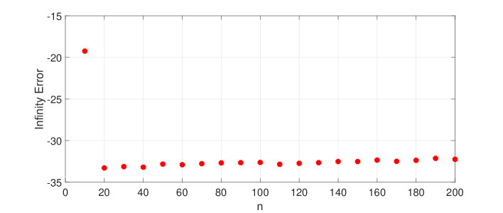
Figure 1: $\|\leavevmode\hbox{\set@color\ignorespaces\verb"expm" }(\textbf{A}_{n})\|_{\infty}$ for $n=10,\ldots,200$

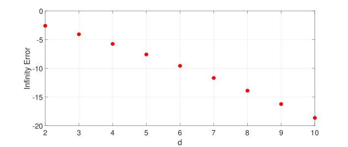
Figure 2: $\|\leavevmode\hbox{\set@color\ignorespaces\verb"E-Ed" }\|_{\infty}$ for $d=2,\ldots,10$

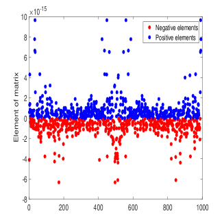
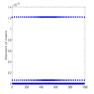
Figure 3: Elements with magnitude less than $10^{-14}$ of $\textbf{A}_{50}$ are computed using command $\leavevmode\hbox{\set@color\ignorespaces\verb"expm" }(\textbf{A}_{50})$(left) and E(right).

7.2 Example 2

Consider the one-dimensional heat equation in $(0,1)$ with homogeneous boundary conditions, $a=1$ and the initial condition

$$u(x,0)=\sin(\pi x).$$

In Figure 4, errors of the present methods with $\Delta x=0.05$, $\mu=2.205$, and $d=8$ are illustrated in time steps by infinity norm. As shown in the figure, error in both methods is similar because the methods are of order $2.$

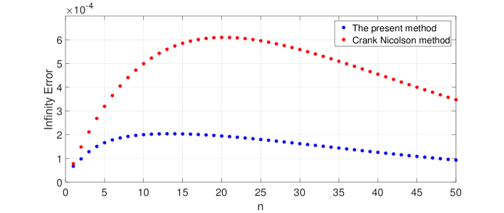
Figure 4: Infinity error of the present method and Crank Nicolson method with $\Delta x=0.05$, $\mu=2.205$, and $d=8$ at $t_{n}=n\Delta t$.

In the next part consider the initial condition

$$u(x,0)=\left\{\begin{array}[]{l l}1&x=0.5\\ 0&\text{otherwise}\end{array}\right.,$$ (7.1)

In Figure 5, the results of the Crank Nicolson are compared with that of the proposed method. From [8] we know the Crank Nicolson method suffers oscillations when $\mu>1$. In this we have chosen $\Delta x=0.04761,\ \Delta t=0.0125$ and $\mu=5$. As we see in Figure 5, the Crank$-$Nicolson method has oscillatory behavior because $\mu$ is greater than $1$, while according to the stability property (7.1) the proposed method provides non-oscillatory solutions.

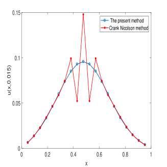
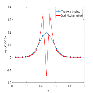
Figure 5: The numerical solutions of one dimensional heat equation with initial condition 7.1 which have a blow up in $x=0.5$ with Crank Nicolson method and the present method at $t=0.005$ (left) and $t=0.015$ (right) with $\mu=5$, $\Delta x=0.04761$ and $d=8$.

7.3 Example 3

In this example consider two-dimensional heat equation with $a=1$, homogeneous conditions on boundary of the unit square $(0,1)^{2}$ with the initial condition

$$u(x,y,t)=\exp(-2\pi^{2}t)\sin(\pi x)\sin(\pi y).$$

In Figure 6 the infinity error of the solution obtained by (6.6) with $d_{1}=d_{2}=10$, $\mu_{x}=\mu_{y}=4.41$, $\Delta t=0.01$ and $\Delta x=0.047$ for $J=20$ and error of Method $1$

$$\textbf{U}^{n+1}=(\verb"expm"[\textbf{L}_{J_{y}-1}]\otimes\verb"expm"[\textbf{T}_{J_{x}-1}])\textbf{U}^{n},$$

and Method $2$

$$\textbf{U}^{n+1,d_{1},d_{2}}=\left(\textbf{K}_{J_{y}-1,d_{2}}\otimes\textbf{G}_{J_{x}-1,d_{1}}\right)\textbf{U}^{n,d_{1},d_{2}}.$$

are plotted for values of $n=1,\ldots,40$. The present method is more accurate since the elements with small magnitude are not calculated accurately using command $\verb"expm"$ as shown in Figure 3.

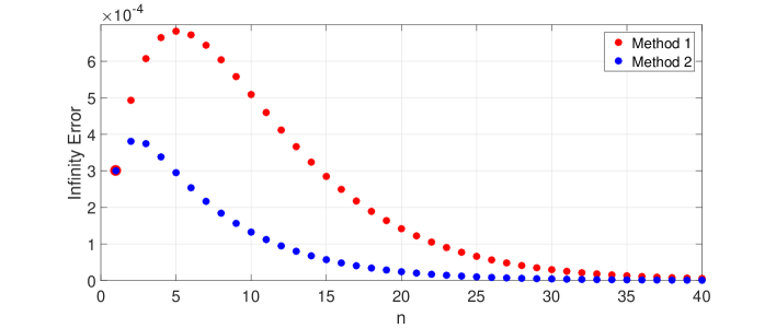
Figure 6: Infinity error of Method 1 and Method 2 with $\Delta x=0.047$, $\mu_{x}=\mu_{y}=4.41$ and $d_{1}=d_{2}=10$ at $t_{n}=n\Delta t$

8 Conclusion

Computing exponential of tridiagonal Toeplitz matrices is an important problem because it has an auxiliary role in the numerical solution of partial differential equations. In this paper, a closed-form approximation based on modified Bessel functions of the first kind is provided and its error is analyzed for these matrices. In the computational view of the problem, elements of the exponential matrix are replaced by only $n+2$ values of Bessel functions of the first kind which are computed independent of $n$, for example by the standard command in MATLAB. This fact reduces CPU time considerably for large matrices.

Besides, a band approximation is derived which is efficient for solving the diffusion equation. Using this idea, new schemes are presented for solving one and two dimension heat equations, stability is investigated and efficiency is examined by comparing it with well-known methods. Also by this idea, an approximation is provided for persymmetric anti-tridiagonal matrices. A generalization of the problem for block Toeplitz tridiagonal matrics is performed.

References

- [1] A. H. Al-Mohy, N. J. Higham, A new scaling and squaring algorithm for the matrix exponential, SIAM J. Matrix Anal. Appl. 31 (2009) 970-989.
- [2] G. B. Arfken, H. J. Weber, Mathematical Methods for Physicists, 6th Edition, Elsevier Academic Press, California, 2005.
- [3] E. Hairer, Ch. Lubich, G. Wanner, Geometric Numerical Integration, Second Edition, Springer Berlin (2000).
- [4] N. J. Higham, Function of Matrices, Theory and Computation, SIAM, Philadelphia, 2008.
- [5] L. Hogben, Handbook of Linear Algebra, CRC Press, Ames, 2013.
- [6] R. Hosseini, M. Tatari, A Diagonal Splitting Method for Solving Semidiscretized Parabolic Partial Differential Equations, Numer Methods Partial Differential Eq. 36 (2020) 268-283.
- [7] C. B. Moler, C. F. Van Loan, Nineteen Dubious Ways to Compute the Exponential of a Matrix, SIAM Review 20 (1978) 801-836. Reprinted and updated as: Nineteen Dubious Ways to Compute the Exponential of a Matrix, Twenty-Five Years Later, SIAM Review 45 (2003) 3-49.
- [8] K. W. Morton, D. F. Mayers, Numerical Solution of Partial Differential Equations, Cambridge University Press, New York, 2005.
- [9] I. Nåsell, Inequalities for modified Bessel functions, Math. Comp. 28 (1974), 253-256.
- [10] S. Noschese, L. Pasquini, L. Reichel, Tridiagonal Toeplitz matrices: properties and novel applications, Numer. Linear Algebra Appl. 20 (2013) 302-326.
- [11] A. Quarteroni, F. Saleri, P. Gervasio, Scientific Computing with MATLAB and Octave, Springer-Verlag, Berlin Heidelberg, New York, 2014.
- [12] Lloyd N. Trefethen, J. A. C. Weideman, The Exponentially Convergent Trapezoidal Rule, SIAM Review, 56 (2014) 385-458.
- [13] Yudell L. Luke, Inequalities for Generalized Hypergeometric Functions, Journal of Approximation Theory, 5 (1972) 41-65.