Local characterization of transient chaos on finite times in open systems

Abstract

To characterize local finite-time properties associated with transient chaos in open dynamical systems, we introduce an escape rate and fractal dimensions suitable for this purpose in a coarse-grained description. We numerically illustrate that these quantifiers have a considerable spread across the domain of the dynamics, but their spatial variation, especially on long but non-asymptotic integration times, is approximately consistent with the relationship that was recognized by Kantz and Grassberger for temporally asymptotic quantifiers. In particular, deviations from this relationship are smaller than differences between various locations, which confirms the existence of such a dynamical law and the suitability of our quantifiers to represent underlying dynamical properties in the non-asymptotic regime.

1 Introduction

Chaotic properties have been traditionally considered in the limit of asymptotically long times [1, 2]. Concentrating on this regime probably has one of its roots in equilibrium statistical physics, in which any macroscopic time scale can be regarded infinitely long compared to the characteristic time scales of the individual components of the system. Furthermore, it may be argued that long-term behavior dominates observations of a system as opposed to initial transients.

A number of approaches is available to characterize chaotic behavior beyond this asymptotic regime (e.g. [3, 4]). One tool is the well-studied finite-time Lyapunov exponent (FTLE, [1, 5]). Besides being a natural approximation to the asymptotic largest positive Lyapunov exponent when only data from a finite time interval are available, its local and location-dependent nature [6] is generally very useful. For example, it is utilized to distinguish between phase-space regions with chaotic and regular dynamics (e.g. [7]), or to identify [5] regions of fluid flow that move in a coherent manner (Lagrangian Coherent Structures, [8, 9]). The spatial variations in the FTLE on which the latter application relies are related to its finite-time nature in that trajectories do not scan the complete accessible part of the phase space. Location dependence can survive even for ergodic systems in the infinite-time limit in association with multifractal features [1, 10], but the clearest expression and usefulness of local properties of chaos appear under a finite-time approach.

In closed flows, generalization to finite time and location dependence of some relationships between chaotic indicators (e.g. entropy and Lyapunov exponent) has been developed in [11]. This was done in the framework of a Ulam-type discretization of the Perron-Frobenius operator of the dynamics [12] in which phase space is partitioned into boxes and averages of the FTLE and its functions within these boxes are computed (thus carrying out coarse-graining). This description, which naturally leads to the use of graph or network methods [12], has been extended to open systems in [13].

In this work, we explore analogous constructions for further quantifiers of open chaotic systems [14]. Open dynamical systems are such that the time evolution of trajectories in the phase space may leave the domain of the dynamics (i.e., where the dynamics is or is chosen to be defined; ’domain’ in what follows). In particular, there is an escape region in the phase space: a trajectory entering there is regarded as escaped. Transient chaos [14] may take place before that escape occurs.

In open chaotic systems, the time evolution of trajectories staying in the domain for long times is governed by a non-attracting chaotic set, either a repeller or a chaotic saddle [1, 14]. However, asymptotic chaotic properties are usually reflected only by a minority of the trajectories uniformly initialized within the domain or within a localized subset thereof. These are the ones initialized sufficiently close to the repeller or to the saddle or its stable manifold. But what happens to the majority of the trajectories? Are there any universal characteristics according to which they leave the domain? In this paper, we will illustrate that local but coarse-grained finite-time quantifiers of chaos provide at least a next-to-asymptotic characterization. Although we are not able to provide a theoretical explanation, we present strong numerical evidence, in the form of a nontrivial fulfillment of the Kantz–Grassberger relation [15], for the meaningful nature of the coarse-grained local finite-time quantifiers which thus give access to analyzing spatial variability in the phase space.

Extending the description of the escape process beyond a restricted minority of trajectories should obviously be useful in practice. Potential applications range from oceanic sedimentation problems to atmospheric dispersion as discussed further in the outlook section (Section 7).

2 Theoretical background for quantifying transient chaos

In this section we recall the standard framework to describe transient chaos in open dynamical systems [14]. Its simplest form is only strictly valid in dynamical systems with a sufficient degree of ergodicity and hyperbolicity, which we will assume in the following. Modifications can be made to deal with more complex systems [1, 14].

The set responsible for chaos, a non-attracting chaotic set, is a union of infinitely many unstable (hyperbolic) periodic trajectories (in particular, they never escape the domain), but this set has zero measure in phase space. If this set repels all trajectories in its neighborhood, it is called a chaotic repeller, whereas if there are also specific directions along which trajectories are attracted, it is called a chaotic saddle [14]. In the following we will usually call the non-attracting chaotic set a saddle, with the understanding that it would in fact be a repeller if stable directions are absent. Motion in the phase space is governed by the invariant manifold or manifolds of the chaotic saddle, i.e., its unstable and (if it exists) stable manifolds. A generic trajectory is guided toward the chaotic saddle along its stable manifold, spends some time by irregularly switching between the neighborhoods of the different unstable periodic orbits, then escapes the domain along the unstable manifold of the chaotic saddle. In the case of a repeller, the first regime, that of an approach to the chaotic set, does not occur.

The strength of chaos is quantified by $\lambda$, the largest positive Lyapunov exponent averaged on the chaotic saddle with respect to its so-called natural probability measure to which the distribution of trajectories trapped on the saddle converges for infinitely long times [14]. Trajectories not moving on the saddle or its stable manifold converge to the unstable manifold of the saddle, distributed according to its so-called conditionally invariant measure [16] in the limit of asymptotically long times. While any of these trajectories eventually escapes the domain, we find such remaining trajectories for arbitrarily long times by considering initial conditions close enough to the saddle or its stable manifold. While their normalized distribution will be described by the conditionally invariant measure, the number $N$ of such trajectories decays exponentially in the asymptotic limit of long times, $N\sim e^{-\kappa t}$, where $\kappa$ is the escape rate [17, 14].

The saddle and its invariant manifolds, as well as the above-mentioned probability measures, have fractal structure. The fractality of the conditionally invariant measure on the unstable manifold is characterized by a collection of fractal dimensions $D_{q}$, $q\in\mathbb{N}$ [18, 14]. The fractal measures corresponding to the stable manifold and the saddle are obtained by identifying the stable manifold with the unstable manifold of the reversed-time dynamics and the saddle with the intersection of the stable and the unstable manifolds, respectively. In dynamical systems preserving phase-space volume, the fractal measures corresponding to the stable and of the unstable manifolds are identical.

A remarkable relationship between the Lyapunov exponents in different unstable directions, the information dimension along them, and the escape rate was obtained by Kantz and Grassberger [15]. For the case of one-dimensional chaotic open maps, for which there is only one Lyapunov exponent $\lambda$, and the chaotic saddle becomes a chaotic repeller of information dimension $D_{1}$, it reads

$$D_{1}=1-\frac{\kappa}{\lambda}\ .$$ (1)

In higher-dimensional chaotic open systems, the relation gets generalized to $\kappa=\sum_{j}\lambda_{j}(1-D_{1}^{(j)})$, where the sum is over the saddle’s unstable directions, of positive Lyapunov exponents $\{\lambda_{j}\}$, and $\{D_{1}^{(j)}\}$ are the partial information dimensions along these directions [15]. Notably, Eq. (1) remains valid for reversible two-dimensional maps.

Kantz and Grassberger [15] justified Eq. (1) and its generalizations in several situations. Here we just quote a simple heuristic argument to arrive at Eq. (1): The trajectories that still remain in the domain of the open map after evolving for a time $t$ need to be initialized very close to the repeller, say within a small distance $\epsilon$. Thus the number of such trajectories (if initialization is uniform in the domain) will be proportional to the number of intervals of size $\epsilon$ covering the repeller multiplied by the interval size $\epsilon$. Using the definition of fractal dimension, the number of such trajectories, $N$, which is proportional to $\exp(-\kappa t)$, should also satisfy $N\propto\epsilon^{1-D}$, or $\kappa t\approx-(1-D)\log\epsilon$. Noting that the interval $\epsilon$ needs to be smaller for longer integration times as $\exp(-\lambda t)$ because of the exponential divergence of trajectories, we immediately arrive at Eq. (1), although a more refined argument [15] is needed to show that the proper dimension to be used is the information dimension $D_{1}$.

Note that $\lambda$, $\kappa$ and $D_{1}$ in Eq. (1) are global quantities of the asymptotic long-time limit (on which their definition relies), i.e., they have a single, unique value for the whole system. In what follows, we shall construct and analyze coarse-grained local finite-time versions of these quantities, and show numerically that a relationship among them similar to Eq. (1) remains valid.

Regarding the Lyapunov exponent, our construction will rely on the FTLE. Alternative non-asymptotic versions, such as the finite-size Lyapunov exponent [19, 20], have also been introduced in the literature. Nevertheless, we focus here on the FTLE, because of the availability of previous analysis that used it in situations involving coarse-graining and escape [11, 13], and, more importantly, because our framework is based on a fixed integration time $T$.

3 Considerations for constructing local finite-time quantifiers

While the success of using the FTLE to learn more about the system than what can be learnt from $\lambda$ alone makes it tempting to introduce corresponding concepts for other quantifiers of chaos, like $\kappa$ and $D_{q}$, there are some important differences which have to be taken into account when constructing the desired local finite-time quantities.

To start with, even infinite-time Lyapunov exponents can be defined locally [21, 2], characterizing the stability of the individual periodic trajectories composing the chaotic set, both in closed and open systems. The variety of the FTLE values obtained for different trajectories reflects this diversity in stability: following a trajectory for a finite time only does not permit the exploration of the complete chaotic set and the incorporation of its typical stability properties. We call this dependence on the initial condition the spatial variation of the FTLE, in the sense that it defines a FTLE value at each point of phase space. This spatial variation is observable and meaningful even in fully chaotic volume-preserving closed systems where the chaotic set fills the entire accessible part of phase space. The spatial variation in open systems is more due to differences in how close different trajectories approach the chaotic saddle, but there should be a range of FTLE values on the saddle as well. Note that, disregarding zero-measure sets (as discussed above) and under standard ergodicity assumptions, location dependence of a quantity in chaos implies its definition to be both local and for finite-time due to the existence of a unique asymptotic probability measure.

Unlike for a local Lyapunov exponent, which is not associated with any probability measure, the definition of the escape rate is inherently linked to the conditionally invariant measure supported by the complete unstable manifold, which appears in the long-time asymptotic limit. This implies that the escape rate is inherently global. While this is an abstract dissimilarity between $\lambda$ and $\kappa$, it is reflected in a more practical difference: whereas the FTLE can be defined and computed along a single trajectory, this does not seem viable for a local finite-time version of the escape rate. Tracking the number of trajectories remaining in the domain requires more than one trajectory. This requirement implies considering boxes of phase space instead of single points as initial conditions, thus performing coarse-graining. Coarse-graining introduces a length scale, $l$, on which it is performed (e.g., $l$ can be the size of the boxes). This length scale can be chosen independently of the properties of the system, and it may be desirable to choose it as small as possible to study location dependence. In principle, one might even try to define and analyze the $l\to 0$ limit, but a finite $l$ is needed for practical purposes, including any numerical computation.

The fractal dimensions $D_{q}$ can theoretically be defined pointwise in phase space [22]. However, once coarse-graining is required to define a proper local escape rate, it appears straightforward to treat the part of the fractal measure of interest that falls into a given box as a single object, and to investigate its dimension according to this choice.

In practice, one partitions the domain $\mathcal{D}$ into boxes $\mathcal{B}_{i}\subset\mathcal{D}$ of size $l$ (‘major boxes’ where distinction from boxes providing further division is needed), and computes every relevant quantity within a single box. We will also take a kind of average of the FTLE within a box, despite the fact that it can be associated with single points in phase space. Note that this coarse graining of the FTLE and its different functions was used in the network-theoretical approach to chaotic transport by fluid flow in [11].

‘Within a box’ only applies to the starting trajectory position: the trajectory is allowed to leave the box and visit the rest of the phase space, not being considered as ‘escaped’ until it leaves the domain $\mathcal{D}$ of the whole dynamical system. That is, we investigate how the trajectories emanating from a localized phase space region experience the influence of the chaotic set.

Once the boxes are given, there are several options to define local finite-time versions of $\kappa$ and $D_{q}$ (see e.g. the discussion about instantaneous and interval-based versions later in this Section). We have chosen definitions such that numerical estimates satisfy a generalized Kantz–Grassberger relation with the smallest deviation. Beyond basic criteria like convergence to the asymptotic definitions, the fulfillment of this relationship ensures that the quantities involved are meaningful.

We denote our coarse-grained local finite-time quantities by $Q_{i}^{(l)}(T;t_{0})$, where $Q$ is the corresponding global quantity, $i$ is the index of the given box ($\mathcal{B}_{i}$), $l$ denotes the coarse-graining scale, $T$ is the length of the finite time interval, and $t_{0}$ is the initialization time for the trajectories $\mathbf{x}_{j}(t)$ with initial locations $\mathbf{x}_{j}(t=t_{0})=\mathbf{x}_{0,j}$, $j=1,\ldots,N_{0}$, in the phase space $\mathcal{X}$. $N_{0}$ is the number of initial conditions. The escape region will be denoted by $\mathcal{E}\subset\mathcal{X}$ (the domain is thus $\mathcal{D}=\mathcal{X}\setminus\mathcal{E}$), and the escape time $\tau_{j}(t_{0})$ of an individual trajectory is defined as

$$\tau_{j}(t_{0})=\min_{t}(t-t_{0})\mid(t\geq t_{0}\land\mathbf{x}_{j}(t)\in\mathcal{E}).$$ (2)

We do not distinguish between flows and maps: the time variables $t$, $t_{0}$, $T$ and $\tau_{j}$ may be regarded to describe discrete time indices, like in our numerical examples. In these examples we omit the indication of $t_{0}$, because the considered dynamical systems does not depend explicitly on time. We emphasize, however, that our definitions are also applicable to nonautonomous dynamical systems, with arbitrary time dependence.

While the definitions should ideally rely on probability measures instead of individual trajectories, we formulate them by means of the latter. We also refer to numbers of trajectories, and implicitly assume being close to the limit of infinitely many trajectories. In particular, the number of trajectories initialized in a box $\mathcal{B}_{i}$ will be denoted by $N_{0,i}$ (with $\sum_{i}N_{0,i}=N_{0}$), and $N_{i}(t;t_{0})$ represents how many of them remain in the domain until time $t$. Formally,

$$N_{0,i} =\sum_{j\mid\mathbf{x}_{0,j}\in\mathcal{B}_{i}}1,$$ (3)

$$N_{i}(t;t_{0}) =\sum_{j\mid\mathbf{x}_{0,j}\in\mathcal{B}_{i}\land\tau_{j}(t_{0})>t-t_{0}}1,$$ (4)

and we call $N_{i}(t;t_{0})/N_{0,i}$ the depletion function. The implicitly assumed limit is defined by $N_{0,i}\to\infty$ with the initial conditions $\mathbf{x}_{0,j}$ uniformly distributed within the given box.

Of course, the quantities should be defined such that they satisfy $\lim_{T\to\infty}Q_{i}^{(l)}(T;t_{0})=Q$ for any initial time $t_{0}$ and any box $\mathcal{B}_{i}$ in autonomous systems; that is, global quantifiers of chaos should be recovered in the limit of asymptotically long times, for any box size, since the asymptotic probability measures should be recovered from any box. Note that this implies that differences between different boxes should decrease for large and increasing $T$.

Like in the case of the traditional FTLE, our finite-time definitions encompass characteristics from the complete time interval from $t_{0}$ to $t_{0}+T$, even though instantaneous characteristics may vary strongly in this period. In particular, the rate of separation of nearby trajectories (lying at the basis of the FTLE) and the rate of escape (the derivative of the logarithm of the depletion function) are typically not constant (cf. Section 5). The case of the fractal dimensions is more complicated, but it is clear that the spatial structure of probability measures forming by $t_{0}+T$ is a result of the time evolution in the complete period between $t_{0}$ and $t_{0}+T$. While we are not currently able to define an “instantaneous fractal dimension”, instantaneous definitions of the Lyapunov exponent and the escape rate are given and numerically investigated in B. Since we conclude that such instantaneous quantifiers numerically fall further from satisfying a Kantz–Grassberger-like relation, we consider and analyze the interval-based versions in the main text. We present our proposals for these definitions in the next Section.

4 Definitions of local finite-time quantifiers

4.1 Lyapunov exponent

For a quantity corresponding to $\lambda$, we should select trajectories that spend a long time near the chaotic saddle, and take the average of the FTLE over all such trajectories initialized within a single major box. This means that we look for trajectories near the stable manifold of the saddle in the given box. We select these trajectories by prescribing that they remain in the domain $\mathcal{D}$ at least for the finite time $T$:

$$\lambda_{i}^{(l)}(T;t_{0})\equiv\frac{1}{N_{i}(t_{0}+T;t_{0})}\sum_{j\mid\mathbf{x}_{0,j}\in\mathcal{B}_{i}\land\tau_{j}(t_{0})>T}\frac{1}{2T}\ln\Lambda(t_{0}+T;\mathbf{x}_{0,j},t_{0}),$$ (5)

where $\frac{1}{2T}\ln\Lambda(t;\mathbf{x}_{0},t_{0})$ is the FTLE evaluated at time $t$ for a trajectory initialized at a position $\mathbf{x}_{0}$ at time $t_{0}$ (i.e., $\Lambda(t;\mathbf{x}_{0},t_{0})$ is the largest eigenvalue of the Cauchy–Green strain tensor $J^{T}J$, with $J=\nabla_{\mathbf{x}_{0}}\mathbf{x}(t)$ being the Jacobian [5]).

4.2 Escape rate

The definition of an escape rate should rely on the number of trajectories remaining in the domain $\mathcal{D}$ up to time $t_{0}+T$, $N_{i}(t_{0}+T;t_{0})$. Since the global escape rate $\kappa$ characterizes the long-term exponential depletion, it is independent of initial transients of transient chaos. As already mentioned, exponential depletion is not observed during these initial transients. It commonly happens that a long time passes until the first trajectory escapes the domain: $N_{i}(t;t_{0})=N_{0,i}$ until then. This might suggest using an instantaneous, differential definition for the finite-time version of $\kappa$ at time $t_{0}+T$ (see B), or one that considers the time of the first escape as initial time, but these constructions will turn out to be inappropriate.

Note that a set of trajectories already undergoes chaotic evolution until the first escape. Thus it is less surprising that we numerically find a more consistent and less biased agreement with a generalized Kantz–Grassberger relation for a definition relying on the original time, $t_{0}$, of initialization.

Our proposed definition reads as

$$\kappa_{i}^{(l)}(T;t_{0})\equiv-\frac{1}{T}\ln\frac{N_{i}(t_{0}+T;t_{0})}{N_{0,i}}.$$ (6)

4.3 Fractal dimensions

Since the dimensions of a saddle and its invariant manifolds are related, and already one of these sets determines the dimensions of the rest in volume-preserving systems, we concentrate on the dimensions related to the stable manifold: we select the trajectories remaining in the system until time $t_{0}+T$, the initial conditions of which represent the stable manifold as observed on this time scale. In the case of a repeller, the same procedure selects the initial conditions sufficiently close to the repeller.

Although fractal dimensions establish a relationship between different length scales (via the scaling of $q$-order Rényi entropies, [23]), their local version must not incorporate properties of trajectories initialized in different boxes. The only option is to resolve length scales below $l$ by partitioning these major boxes by the introduction of minor boxes, the size of which we denote by $\varepsilon\leq l$.

The finite-time nature of the desired quantity does not allow resolving arbitrarily small scales either. The initial conditions of the trajectories remaining in the domain until $t_{0}+T$ will not exhibit self-similar structures below a certain length scale. Instead, they will exhibit a space-filling pattern if investigated on a sufficiently small scale. What corresponds to the effects of chaotic trajectory evolution is observed on scales between this space-filling regime and the largest accessible length scale, $l$. Even in this intermediate regime, exact self-similarity and a well-defined scaling exponent for Rényi entropies is not expected to be found, so that the crossover between the intermediate and the space-filling regimes (down to which fractality “reaches”), labelled by $\varepsilon^{*}$, may be difficult to identify.

One source of the erratic scaling of Rényi entropies with $\varepsilon$ is that box boundaries arbitrarily introduced will not match the geometry of the fractal. This particular issue can be worked around by recognizing that different choices of box boundaries for a given box size should yield equally relevant results. For simplicity we consider in the following the simple situation in which all major and minor boxes are hypercubes of the same large and small sizes, respectively. We see that one problem in this simple framework is that partitioning a major box of size $l$ uniformly to a number $n$ of minor boxes of size $\varepsilon$ (assuming that $l$ is an integer multiple of $\varepsilon$) is possible in only one way. Any relocation of box boundaries results in partial minor boxes at the edges of the major box. To consistently take into account the contribution from such partial minor boxes, we generalize the $q$-order Rényi entropy (writing it in the case of a one-dimensional phase space for definiteness) as

$$H_{q}^{\prime}(f_{0})=\frac{1}{1-q}\ln\sum_{k=0}^{n}f_{k}\left(\frac{p_{k}}{f_{k}}\right)^{q}.$$ (7)

The standard Rényi entropy is recovered when $f_{k}=1$ $\forall k\neq 0$. The sum is over all minor boxes inside a fixed major one, and $p_{k}$ is the relative measure of the $k$th minor box with respect to the total measure of the full major box (i.e., $\sum_{k}p_{k}=1$). We take $f_{k}=1$ for $k\in\{1,\ldots,n-1\}$, i.e., for all entire minor boxes, and $f_{0}$ and $f_{n}$ give the ratio of the length of the first and the last (partial) minor box, respectively, to that of the entire minor boxes. Note that we have $n+1$ minor boxes in total, $f_{n}=1-f_{0}$, and the boundary configuration in this kind of partitioning is completely characterized by $f_{0}\in[0,1)$. By the generalization (7), we linearly extrapolate the average probability density within partial boxes to the size of entire boxes, and, furthermore, recover Rényi entropies for all $q$ in the case of a uniform probability distribution.

In a second step, to take into account all possible boundary configurations with equal weight, we take the mean of this generalized $q$-order Rényi entropy over the possible box boundary configurations:

$$\overline{H_{q}^{\prime}}=\int_{0}^{1}H_{q}^{\prime}(f_{0})\mathrm{d}f_{0}.$$ (8)

Constructing the corresponding definitions for more than one dimension is straightforward, as well as extending the approach to box-boundary configurations not relying on a uniform partitioning to $n$ minor boxes. We utilize these mean generalized Rényi entropies in our below definition of local finite-time fractal dimensions.

While our approach smoothes out the erratic scaling of Rényi entropies with $\varepsilon$ very effectively, an intermediate regime in $\varepsilon$ with power-law scaling is still not found (due to the effects of initial transients in trajectory evolution right after $t_{0}$, cf. Sects. 3 and 5), so that the identification of $\varepsilon^{*}$ remains unsolved.

For this identification, we have to rely on empirical numerical findings in the setup of Sect. 5. As we will describe in detail in A for that numerical setup, the slope of $\overline{H_{1}^{\prime}}$ as a function of the logarithm of the minor box size $\varepsilon$ turns out to converge to $1$ (corresponding to space filling) for decreasing $\varepsilon$ following a power law with exponent $-1$ in any major box. We take the smallest value of $\overline{H_{1}^{\prime}}$ below which this scaling is observed for all integration times $T$ in the numerically accessible range for the given major box, and select $\varepsilon^{*}$ for each $T$ as the value of $\varepsilon$ corresponding to that $\overline{H_{1}^{\prime}}$. We regard this algorithm as part of our definition, but we acknowledge that it is not a complete one from a theoretical point of view.

For the formulation of these definitions, we assume now that a unique $\varepsilon^{*}$ exists for the approximate stable manifold of the saddle (or for the approximate repeller) obtained for given $T$ and $t_{0}$ in a box $\mathcal{B}_{i}$. Our definition, encompassing the entire interval in length scales between $l$ and $\varepsilon^{*}$, is

$$D_{q,i}^{(l)}(T;t_{0})\equiv-\frac{\overline{H_{q}^{\prime}}^{(\varepsilon^{*})}-\overline{H_{q}^{\prime}}^{(l)}}{\ln(\varepsilon^{*}/l)}$$ (9)

where $\overline{H_{q}^{\prime}}^{(\varepsilon)}$ is the mean generalized $q$-order Rényi entropy (8) taken for minor boxes of size $\varepsilon$ for the approximate stable manifold obtained for given $T$ and $t_{0}$ in a box $\mathcal{B}_{i}$.

With appropriate dynamical and geometric ingredients, we conjecture the generalization of the Kantz-Grassberger relation to local and finite-time quantities in one- and two-dimensional maps:

$$D_{1,i}^{(l)}(T;t_{0})=1-\frac{\kappa_{i}^{(l)}(T;t_{0})}{\lambda_{i}^{(l)}(T;t_{0})}\ .$$ (10)

We will check in the following Section how closely this formula is satisfied with the definitions of the present Section.

5 Numerical results

For our numerical investigations, we take the logistic map as in [15], which is a well-studied autonomous non-invertible one-dimensional map. In our analyses, we regard time as discrete, choose $t_{0}=0$, and omit $t_{0}$ in the notation.

The mentioned version of the logistic map reads

$$x_{t+1}=1-ax_{t}^{2}\ ,$$ (11)

with $a=1.75487767$, and it is defined on the phase space $\mathcal{X}=[-1,1]$. Escape is considered here to the period-3 attractor. In order to be able to define an escape region $\mathcal{E}$, and at variance with [15], leaks of width $w$ are introduced and centered on the positions corresponding to the period-3 trajectory [16, 17]: $\mathcal{E}=\cup_{k\in\{1,2,3\}}(x^{(k)}-w/2,x^{(k)}+w/2)$, where $x^{(k)}$ is the $k$th point of the attracting period-3 trajectory (marked with dots on the horizontal axes of Fig. 2). We choose $w=0.04$, a rather small value to approximately conform with the approach of [15].

For coarse-graining, we partition the phase space $\mathcal{X}=[-1,1]$ uniformly to an integer number of boxes $\mathcal{B}_{i}$, but ignore the boxes containing the leaks. We also ignore the boxes from which all trajectories escape within a given $T$ in the numerical simulations, since the local finite-time Lyapunov exponent and escape rate are not meaningful for these boxes.

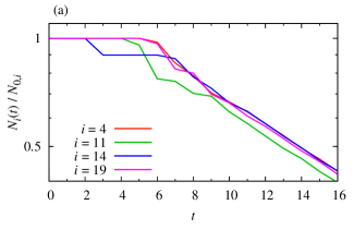
(a)

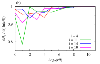
(b)

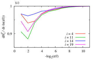
(c)

Figure 1: Examples for the depletion function (a) and for the slope of $H_{1}$ (b) and $\overline{H_{1}^{\prime}}$ (c) with respect to the logarithm of the minor-box size (the limit $\varepsilon\to 0$ is approached towards the right of the plot) as numerically obtained in the logistic map (11). Four different major boxes $\mathcal{B}_{i}$ are shown. $i$ increases from the left boundary of the interval $[-1,1]$, and the major-box size is $l=0.04$ (thus $l=w$). $T=7$ for panels (b) and (c).

We first present numerical results in Fig. 1a for the depletion function $N_{i}(t;t_{0})/N_{0,i}$ in some boxes selected as examples. The depletion function (Fig. 1a) tends to be constant at the beginning. While it becomes exponential for $t>11$ approximately, its shape between the initial constant and the asymptotic exponential regime varies much between different boxes and can be rather complicated. That is, the escape process is definitely not yet governed by the conditionally invariant measure for $t<11$.

For an example of the scaling of $\overline{H_{1}^{\prime}}$, we will take a time instant from the intermediate regime, $t=T=7$, when escape is already considerable but its properties are not yet asymptotic. For reference, we first show in Fig. 1b the corresponding scaling of the standard Rényi entropy $H_{1}$ (Eq. (7) with $f_{0}=0$ and $f_{k}=1$ for all $k\neq 0$) with $\varepsilon$. As expected, space-filling is observed for small $\varepsilon$ at our choice of a finite time. From the major-box size ($\varepsilon=l$) to the space-filling regime, however, scaling appears to be completely erratic. In view of this observation, it is remarkable to see in Fig. 1c that the scaling of $\overline{H_{1}^{\prime}}$ is much smoother. Typical properties seem to be a weaker slope for large $\varepsilon$ and a gradual approach of the space-filling regime. However, where this gradual, universal-looking approach begins depends on the chosen box $i$, and irregularities are still observable before the beginning of this gradual approach. These irregularities are most pronounced in the example of $i=14$, but also note the break at $\varepsilon/l=2^{-6}$ for $i=11$, and that the otherwise similar-looking lines for $i=4$ and $i=19$ cross each other. We explain in A that we use the gradual approach (which numerically turns out to be a power law with exponent $-1$) towards space-filling to identify $\varepsilon^{*}$ separately in each box but utilizing all accessible time intervals $T$, as already explained in Sect. 4.3. We also illustrate in A that the characteristic properties of the finite-time escape process are mainly linked to the irregular regime. This appears to be so in spite of the fact that the irregularities imply the absence of a self-similar scaling.

While the meaningful characterization of the asymptotic escape relies on the fractality of the conditionally invariant measure and on the corresponding exponential depletion of the domain, Fig. 1 suggests that the finite-time behavior is qualitatively different. See also the last paragraph of Section 3, where the particular choice of the definitions (5) and (6) is explained.

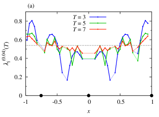
(a)

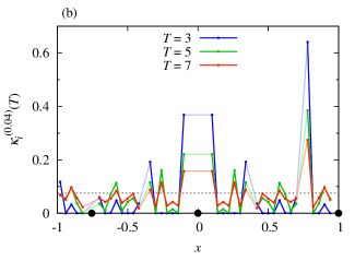
(b)

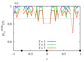
(c)

Figure 2: The coarse-grained local finite-time Lyapunov exponent (a), escape rate (b), and information dimension (c) in different major boxes $\mathcal{B}_{i}$ along the $x$ axis as numerically obtained in the logistic map (11). The positions $x^{(k)}$, $k\in\{1,2,3\}$, corresponding to the attracting period-3 trajectory, on which the leaks of width $w=0.04$ are centered, are marked by black dots. The box size for coarse-graining is $l=0.04$. The values are connected with lines to guide the eye (lines are fainter over ignored boxes, see text). Different values of $T$ are taken as indicated in the legend. The asymptotic global values, $\lambda=0.54$, $\kappa=0.075$ and $D_{1}=0.86$, are included as gray dashed horizontal lines.

Numerical results for the different local finite-time quantifiers are shown in the different panels of Fig. 2, for various $T$ but for a given $l$. Location dependence is indeed observed for all quantifiers and looks irregular, apart from the symmetry (except for the leaks) to the point $x=0$, which results from the invariance of the time evolution to the sign change of an initial condition. With increasing $T$, this location-dependence is generally attenuated, and the quantifiers approach the asymptotic global values, as expected. (The asymptotic global values have been computed by regarding the whole phase space as a single box. For $\lambda$ and $\kappa$, the formulae of B, (B.1) and (12), influenced less by initial transients, have been utilized with $T=80$. For $D_{1}$, the slope of $\overline{H_{1}^{\prime}}$ has been taken at $\varepsilon/l=2^{-15}$ for $T=40$.) There are a few boxes in Fig. 2c for which convergence is not observed. In these boxes and some further ones, most trajectories escape within a very short time, which makes numerical analyses difficult. We also have boxes $i$ from which no trajectories escape up to $T$ and where, consequently, $\kappa_{i}^{(l)}(T)=0$ and $D_{1,i}^{(l)}(T)=1$.

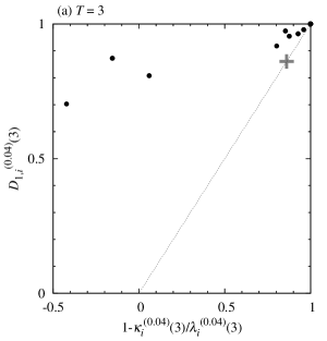
(a)

(b)

(c)

(d)

Figure 3: Relationship between the coarse-grained local finite-time version of the quantities appearing in the local Kantz–Grassberger relation (10) as numerically obtained in the logistic map (11), for $T=3,5,7,10$ as indicated in the panels. In every panel, each data point corresponds to a single major box $\mathcal{B}_{i}$ with $i$ running from $1$ to $50$ but skipping boxes overlapping with leaks or from which all trajectories escape by $T$. The size of the boxes is $l=0.04$. The Kantz–Grassberger relation is represented by the diagonal line. The gray cross marks the point that corresponds to the asymptotic global values $\lambda=0.54$, $\kappa=0.075$ and $D_{1}=0.86$.

In Fig. 3 we check the generalized Kantz–Grassberber relation for different times. It illustrates that for small $T$ there are boxes for which the quantifiers are rather far from satisfying the local Kantz–Grassberger relation, Eq. (10), biased to the upper side of the diagonal representing this relation. The largest biases, resulting in negative horizontal coordinates in some cases, correspond to boxes with rapid escape mentioned in the previous paragraph. (Note, however, that biases are generally still smaller than deviations in the plots of B.) Of course, the quantifiers of boxes without escaping trajectories fall to the upper right corner and thus satisfy the local Kantz–Grassberger relation. For increasing $T$, data points not falling to this corner generally get closer to the diagonal, which may be regarded natural in view of the convergence of all quantifiers to the asymptotic values as seen in Fig. 2. However, the pattern according to which the different boxes $\mathcal{B}_{i}$ approximate the relation is not at all erratic, especially for large $T$. In particular, the approximations originating from the different boxes are organized close to the diagonal (although still exhibiting a little bias), and for large $T$ (Figs. 3c-3d) they have a spread much broader than the distances of the individual data points from the diagonal, confirming the relevance of Eq. (10) to describe the still non-asymptotic behavior at this $T$. For increasing $T$, the spread of the data points along the diagonal somewhat decreases, too, as they get closer to the point representing the asymptotic values.

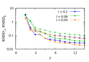
Figure 4: RMSD_⟂ (solid) and RMSD_∥ (dashed; see text) as a function of the integration time $T$, for different values of the box size $l$.

We quantify these last observations by considering the distance of each data point from the diagonal, and also the distance of its projected position on the diagonal from the point representing the asymptotic global values. (Numerically, both coordinates of the latter point are taken to be $1-\kappa/\lambda$ for this analysis, since it can be computed more precisely than $D_{1}$.) We then take the root mean square of these distances, RMSD_⟂ and RMSD_∥, over all boxes to obtain aggregated quantifiers of the deviation from the local Kantz–Grassberger relation and from the asymptotic values, respectively. According to Fig. 4, both quantifiers of deviation decay with increasing $T$, and RMSD_⟂ indeed decays faster than RMSD_∥, not only for $l=0.04$ as in Fig. 3, but also for other choices of $l$. Although the dependence on $l$ is not monotonic, the deviations are the smallest for the smallest $l$.

(a)

(b)

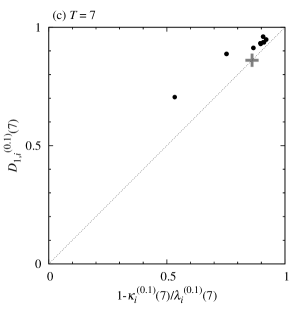
(c)

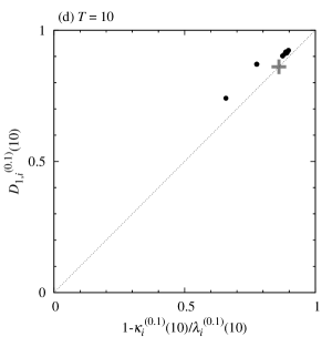
(d)

Figure 5: Same as Fig. 3 for $l=0.1$.

For a larger $l$, the general pattern of the scatter plot between the quantities on the two sides of Eq. (10), presented in Fig. 5, remains the same as in Fig. 3, indicating the robust nature of our numerical findings. However, as expected from Fig. 4, the Kantz–Grassberger relation is satisfied with less accuracy, which might suggest that properly resolving location dependence might be important.

6 Discussion

The construction of coarse-grained local finite-time quantifiers of transient chaos presented in this paper may appear somewhat ad-hoc, especially due to the lack of a firm theoretical foundation. The complete lack of exponential and power-law functional forms for the depletion function and the entropy scaling from $t_{0}$ to $t_{0}+T$ and from $l$ to $\varepsilon^{*}$, respectively, as numerically found in Fig. 1, may raise doubts if the quantifiers as defined in Section 4 are meaningful at all. The convergence to the asymptotic values and to satisfying the Kantz–Grassberger relation for increasing $T$ is just a minimal requirement. However, the numerical observation of Fig. 3 about the diagonal alignment of data points representing different boxes provides an indication of the existence of a non-asymptotic dynamical relationship, Eq. (10), in localized regions of the phase space. It is possible that this relationship is not best caught by our quantifiers, and one might be able to find more appropriate definitions. However, our numerical experience does imply that these quantifiers characterize some properties of chaotic escape at least when approaching but not reaching the asymptotic regime with $T$.

The existence of a non-asymptotic relationship Eq. (10), a dynamical law, may be even more interesting from a theoretical point of view. In a short formulation, this law states that coarse-grained but localized chaotic properties of finite time scales vary across the domain such that they approximately satisfy the Kantz–Grassberger formula everywhere. Unfortunately, we are not able to provide a firm demonstration for this. As a consequence, we are not able to assess the validity range.

We numerically show that the formula is satisfied better for increasing $T$. While this might suggest later behavior to be more relevant for the relationship, we recall that utilizing temporally instantaneous quantifiers (except for the fractal dimension) results in a worse agreement with the relationship for any $T$ (see B). This might indicate that encompassing the full history from the initial time $t_{0}$ would be important.

On the other hand, trajectories that escape the domain very early do not exhibit any chaotic behavior. Their time evolution and escape are expected to be determined by the global phase space structure of the system instead of properties of the non-attracting chaotic set. Therefore, it is quite plausible that no universal relationship exists between quantifiers of chaos for small $T$, and that these quantifiers do not really “tell” anything about the system in this case. Since, as mentioned in the introduction, most of the trajectories escape early, we might simply be lacking universal laws describing the behavior of the majority of the trajectories. The relationship discovered in this paper may prove to be a next-to-leading-order phenomenon before asymptotics is reached.

In our heuristic arguments we have assumed hyperbolic behavior for the open chaotic system. Theoretical considerations concerning non-hyperbolic systems are intrinsically more complex since they lack the universality of hyperbolic ones. Nevertheless, a feature of most non-hyperbolic open systems is that the exponential decay of the depletion function is replaced by power-law decay at long times, so that the asymptotic escape rate is zero. But still in this case the Kantz-Grassberger relationship is satisfied, because the chaotic saddle becomes locally space filling in non-hyperbolic regions and its dimension the one of the full domain [14]. In addition, the non-exponential decay appears only after a long transient during which the dynamics usually has the features of hyperbolic systems. We are considering a finite-time regime even earlier than that. For these reasons, and although we neither can provide a firm theoretical justification nor have performed numerical tests, we expect our conclusions on the validity of the generalization of the Kantz-Grassberger relationship to hold also in non-hyperbolic situations.

7 Outlook

Numerically, the coarse-grained local finite-time Lyapunov exponent and escape rate are straightforward to compute. Once local finite-time properties of the chaotic escape of trajectories are characterized by these quantifiers, one may use the discovered relationship to draw conclusions about the corresponding fractality, i.e., of the spatial organization of the trajectories involved. This relationship, a generalization of the Kantz-Grassberger relation, relates dynamical and geometrical quantities in chaotic flows in non-asymptotic regimes, and may thus be relevant in practical situations in which infinite-time limits are never reached.

From a practical point of view, these quantifiers might be even more useful to learn about differences in the rate of escape and the spatial organization of trajectories emanating from different regions of the domain in association with a given time scale $T$.

We envisage applications in the characterization of the structures generated during oceanic sedimentation processes [24, 25, 26] or atmospheric dispersion [27]. The approach is especially suited for the assessment of the spreading of pollutants originating from localized emissions [28].

Finally, we briefly remark on the relation of our quantifiers to network characteristics. As discussed in [11] (see also [12]), the boxes of the phase space used for coarse-graining can be regarded as nodes of a directed weighted network [29], where the link weights are defined by the number of trajectories starting in one box and finishing in the other one after a given integration time, properly normalized. For open systems, [13] already showed a correspondence between the box-based FTLE and the out-degree of the given box in this network. Our definition (6) for the coarse-grained local finite-time escape rate is recognized to be precisely the out-strength of the given box. As for the fractal dimensions (9), a network-theoretical counterpart can hardly be imagined, since our definition relies on internal properties of the box. However, the fulfillment of the Kantz–Grassberger relation between the coarse-grained local finite-time information dimension and the previous two quantities emphasizes the relevance of this dimension on scales above the box size and thus for the dynamics represented by the network. Potential applications of this framework are yet to be explored.

Data availability statement

The data that support the findings of this study are available upon reasonable request from the authors.

Appendix A How to identify $\varepsilon^{*}$

Our algorithm for the identification of an apparently suitable value of $\varepsilon^{*}$ is solely based on numerical results. Nevertheless, our numerical experience seems robust, and we believe that our algorithm, otherwise constructed along heuristic reasoning, provides a meaningful $\varepsilon^{*}$.

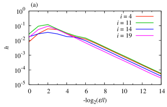
(a)

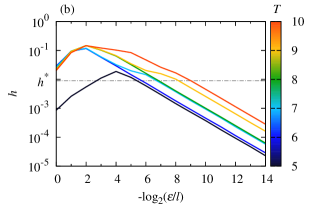
(b)

Figure 6: Examples for $h=1-\mathrm{d}\overline{H_{1}^{\prime}}/\mathrm{d}(-\ln(\varepsilon/l))$ as numerically obtained in the logistic map (11) in different boxes $\mathcal{B}_{i}$ for $T=7$ (a) and for different values of $T$ in box $i=11$ (b). The box size is $l=0.04$. $h^{*}$ is marked by a dot-dashed line in panel (b): below $h^{*}$, the lines appear completely straight for decreasing $\varepsilon^{*}$ for all values of $T$ (see text for details).

In Fig. 1b of Section 5, we found a gradual approach of the space-filling regime for decreasing $\varepsilon$ in the scaling of $\overline{H_{1}^{\prime}}$. In Fig. 6a, we plot the same data on a logarithmic scale transformed as $h=1-\mathrm{d}\overline{H_{1}^{\prime}}/\mathrm{d}(-\ln(\varepsilon/l))$ so that the nature of this gradual approach becomes clear: numerically, it is evident that $h$ converges to the space-filling regime for decreasing $\varepsilon$ according to a power law with exponent $-1$, independently of the chosen box $\mathcal{B}_{i}$. We prefer not providing with an explanation, but accepting this as numerical evidence.

Within the regime of this power-law approach, obviously, no crossover point can be defined where the scaling of $\overline{H_{1}^{\prime}}$ would enter the space-filling regime. Furthermore, since the approach follows the same power law for all boxes, it cannot give information about differences in the scaling of $\overline{H_{1}^{\prime}}$ between different locations within the domain. Consequently, it might appear to be reasonable to exclude the regime of power-law approach from the definition of the coarse-grained local finite-time fractal dimension, and place $\varepsilon^{*}$ where the power-law regime begins.

In Fig. 6b, we compare the scaling of $\overline{H_{1}^{\prime}}$ via its transform $h$ for different lengths $T$ for a single box chosen as an example. Apart from approaching the space-filling property at increasingly smaller values of $\varepsilon$ for increasing $T$ (the lines shift to the right), which is rather natural given that the shape of the ensemble of trajectories emanating from a box becomes more and more complicated with time evolution, it also becomes obvious that several different sections of apparent non-power-law and power-law approach may be present for a single $T$ (see e.g. $T=7$, where power-law sections are found near $\varepsilon/l=2^{-3}$ and below $\varepsilon/l=2^{-6}$ with non-power-law sections in between and for large $\varepsilon$) and that such sections may appear, disappear and reappear for different values of $T$. Since any deviation from a power law may carry unique information for a given box $\mathcal{B}_{i}$, only the last power-law section in $h$ can be relevant for the identification of $\varepsilon^{*}$. However, as Fig. 6b illustrates, the beginning of this last section varies very much between different values of $T$ due to the irregular introduction of non-power-law sections, so that it might well be that not the entirety of the last power-law section is relevant.

According to our numerical experience, like in Fig. 6b, there is a value $h=h^{*}$ below which one always (for all values of $T$) finds only power-law behavior. The section below $h^{*}$ should thus reliably reflect universal and scale-free properties of the approach of the space-filling pattern. We decided to identify $h^{*}$ based on the accessible lengths $T$ in our numerics and to choose $\varepsilon^{*}$ separately for each $T$ as the smallest value of $\varepsilon$ for which $h(\varepsilon;T)>h^{*}$.

For selecting $h^{*}$, we first fit least-squares lines (in logarithmic coordinates), separately for each $T$, of increasing length to the smallest numerically accessible part of $h(\varepsilon;T)$, and identify where the deviation from the linear shape increases the most between two consecutive fitting steps. [In particular, we compute the logarithm of the root mean square deviation in each fitting step (each step includes one more data point at the larger end of the $\varepsilon$ interval for fitting), and find the step where this logarithm increases the most such that the new fitted slope deviates from 1 more than the slope fitted in the previous step.] The value of $h$ that just neighbors the one where the largest increase has been identified gives a candidate for $h^{*}$ for each $T$. As the final $h^{*}$, we simply select the minimum of these individual values.

Appendix B Instantaneous definitions

B.1 Definitions

After long-enough time $T$ from initialization, trajectories remaining in the domain are distributed according to the conditionally invariant measure and are thus escaping the domain at a constant rate. This rate, not influenced by initial transients, is captured by the time derivative of the logarithm of the depletion function for any box. Therefore, as an extension of this concept, we define the instantaneous version of $\kappa_{i}^{(l)}(T;t_{0})$ for an arbitrary time interval $T>0$ as

$$\tilde{\kappa}_{i}^{(l)}(T;t_{0})=-\frac{\mathrm{d}}{\mathrm{d}t}\left.\left(\ln\frac{N_{i}(t;t_{0})}{N_{0,i}}\right)\right|_{t=t_{0}+T}.$$ (12)

The reason why a trajectory remains within the domain for a long time $T$ typically is that it stays long in the vicinity of the saddle (or repeller) before escaping, visiting different parts of the phase space according to the natural measure of the saddle. During such a time evolution, nearby trajectories diverge according to $\lambda$, the average largest positive Lyapunov exponent. Although the rate of divergence fluctuates in time for any given pair of trajectories, $\lambda$ can be recovered at a single time instant $t^{\prime}$ by averaging over an ensemble of trajectories. Such an ensemble can be obtained by initializing trajectories in any box but keeping only those that stay in the domain long after $t^{\prime}$ (one may consider e.g. those with $T=2(t^{\prime}-t_{0})$ with $T$ sufficiently large, cf. the sprinkler method for the visualization of the saddle, [30]). The rate of divergence can be computed via time differentiation instead of taking into account the complete interval from initialization. In this case, again, initial transients do not affect the behavior of trajectories at $t^{\prime}=t_{0}+T/2$ for large $T$. With this limiting case in mind, we define the instant-based counterpart of $\lambda_{i}^{(l)}(T;t_{0})$ for a specified box $\mathcal{B}_{i}$ as

$$\tilde{\lambda}_{i}^{(l)}(T;t_{0})=\frac{1}{N_{i}(t_{0}+T;t_{0})}\times$$

$$\sum_{j\mid\mathbf{x}_{0,j}\in\mathcal{B}_{i}\land\tau_{j}(t_{0})>T}\lim_{\Delta t\to 0}\frac{1}{2\Delta t}\ln\Lambda\left(t_{0}+\frac{T}{2}+\Delta t;\mathbf{x}_{j}\left(t_{0}+\frac{T}{2}\right),t_{0}+\frac{T}{2}\right).$$ (13)

Note that the quantity in the sum is a finite-time Lyapunov exponent, but evaluated over an infinitesimal time interval $\Delta t$ starting from the position of the trajectory $j$ at time $t_{0}+T/2$. While the above formulation is for flows, the time derivatives should be replaced by finite differences for maps.

B.2 Numerical observations

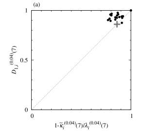
(a)

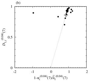
(b)

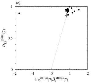
(c)

Figure 7: Same as Fig. 3c with intantaneous quantities as indicated on the axes. The gray cross marks the point that corresponds to the asymptotic global values $\lambda=0.54$, $\kappa=0.075$ and $D_{1}=0.86$.

In Fig. 7, we replace one or both of $\lambda_{i}^{(l)}(T;t_{0})$ and $\kappa_{i}^{(l)}(T;t_{0})$ by their instantaneous counterpart. Agreement with the generalized Kantz–Grassberger relation, Eq. (10), is much worse than in Fig. 3c in any combination. The cloud of points representing the different boxes generally looks unstructured, and signs of aligning to the Kantz–Grassberger relation are never observed, in contrary to Fig. 3c. When $\tilde{\lambda}_{i}^{(l)}(T;t_{0})$ is used in place of $\lambda_{i}^{(l)}(T;t_{0})$ (Figs. 7b and 7a), it turns out to be negative for some boxes. The observation of an unstructured cloud of points for $\tilde{\kappa}_{i}^{(l)}(T;t_{0})$ and $\lambda_{i}^{(l)}(T;t_{0})$ (Fig. 7a) stresses the non-triviality of the agreement observed in Fig. 3c: using quantifiers with a correct asymptotic limit is not sufficient to guarantee that Eq. (10) is satisfied in any pre-asymptotic regime.

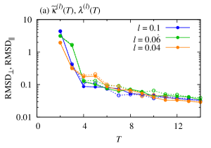
(a)

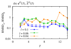
(b)

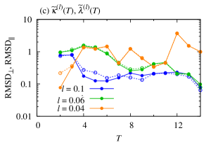
(c)

Figure 8: Same as Fig. 4 with intantaneous quantities as indicated in the panels.

The lack of the alignment of the cloud of points is also indicated by the nearly same magnitude of RMSD_⟂ and RMSD_∥ in Fig. 8 which is the analogue of Fig. 4 with different combinations of the instantaneous quantifiers. The deviation from the Kantz–Grassberger relation in RMSD_⟂ is generally larger in Fig. 8a than in Fig. 4, and there is no convergence with increasing $T$ to the asymptotic values in Figs. 8c and 8a. These observations justify the choices of Sect. 4.

References

References

- [1] Ott E 2002 Chaos in dynamical systems, 2nd Edition (Cambridge University Press, Cambridge, UK)
- [2] Tél T and Gruiz M 2006 Chaotic Dynamics: An Introduction Based on Classical Mechanics (Cambridge University Press, Cambridge, UK)
- [3] Boffetta G, Celani A, Cencini M, Lacorata G and Vulpiani A 2000 Chaos: An Interdisciplinary Journal of Nonlinear Science 10 50–60
- [4] Boffetta G, Cencini M, Falcioni M and Vulpiani A 2002 Physics Reports 356 367–474
- [5] Shadden S C, Lekien F and Marsden J E 2005 Physica D: Nonlinear Phenomena 212 271 – 304 ISSN 0167-2789
- [6] Wolff R C L 1992 Journal of the Royal Statistical Society: Series B (Methodological) 54 353–371
- [7] Pierini S, Ghil M and Chekroun M D 2016 Journal of Climate 29 4185–4202 ISSN 0894-8755
- [8] Haller G and Yuan G 2000 Physica D: Nonlinear Phenomena 147 352 – 370 ISSN 0167-2789
- [9] Peacock T and Dabiri J 2010 Chaos: An Interdisciplinary Journal of Nonlinear Science 20 017501
- [10] Neufeld Z and Hernández-García E 2010 Chemical and Biological Processes in Fluid Flows: A Dynamical Systems Approach (Imperial College Press, London, UK)
- [11] Ser-Giacomi E, Rossi V, López C and Hernández-García E 2015 Chaos: An Interdisciplinary Journal of Nonlinear Science 25 036404
- [12] Bollt E M and Santitissadeekorn N 2013 Applied and Computational Measurable Dynamics (SIAM, Philadelphia, USA)
- [13] Ser-Giacomi E, Rodríguez-Méndez V, López C and Hernández-García E 2017 The European Physical Journal Special Topics 226 2057–2068
- [14] Lai Y C and Tél T 2011 Transient chaos (Springer, New York, USA)
- [15] Kantz H and Grassberger P 1985 Physica D: Nonlinear Phenomena 17 75 – 86 ISSN 0167-2789
- [16] Pianigiani G and Yorke J A 1979 Trans. Amer. Math. Soc. 252 351–366
- [17] Altmann E G and Tél T 2009 Phys. Rev. E 79(1) 016204
- [18] Farmer J, Ott E and Yorke J A 1983 Physica D: Nonlinear Phenomena 7 153 – 180 ISSN 0167-2789
- [19] Aurell E, Boffetta G, Crisanti A, Paladin G and Vulpiani A 1997 Journal of Physics A: Mathematical and General 30 1–26
- [20] Bettencourt J H, López C and Hernández-García E 2013 Journal of Physics A: Mathematical and Theoretical 46 254022
- [21] Eden A 1989 ESAIM: Mathematical Modelling and Numerical Analysis - Modélisation Mathématique et Analyse Numérique 23 405–413
- [22] Grebogi C, Ott E and Yorke J A 1988 Phys. Rev. A 37(5) 1711–1724
- [23] Renyi A 1970 Probability theory (North-Holland, Amsterdam, the Netherlands)
- [24] Monroy P, Hernández-García E, Rossi V and López C 2017 Nonlinear Processes in Geophysics 24 293–305 URL https://npg.copernicus.org/articles/24/293/2017/
- [25] Monroy P, Drótos G, Hernández-García E and López C 2019 Journal of Geophysical Research: Oceans 124 4744–4762
- [26] Sozza A, Drótos G, Hernández-García E and López C 2020 Physics of Fluids 32 075104
- [27] Haszpra T 2019 Chaos: An Interdisciplinary Journal of Nonlinear Science 29 071103
- [28] Haszpra T and Tél T 2011 Journal of Physics: Conference Series 333 012008
- [29] Newman M 2010 Networks: An Introduction (Oxford University Press, Oxford, UK)
- [30] Hsu G H, Ott E and Grebogi C 1988 Physics Letters A 127 199 – 204 ISSN 0375-9601