Dirac particles on periodic quantum graphs

Abstract

We consider the Dirac equation on periodic networks (quantum graphs). The self-adjoint quasi periodic boundary conditions are derived. The secular equation allowing us to find the energy spectrum of the Dirac particles on periodic quantum graphs is obtained. Band spectra of the periodic quantum graphs of different topologies are calculated. Universality of the probability to be in the spectrum for certain graph topologies is observed.

I Introduction

Quantum graphs have attracted much attention as an effective tool for modeling particle and wave dynamics in branched quantum structures. The advantage of quantum graphs in modeling quantum transport in low-dimensional branched structures and networks comes from the fact that the description can be effectively reduced into a one-dimensional Schrödinger (Dirac) equation on metric graphs, which can be exactly solved in most of the cases. Quantum graphs are determined as the branched quantum wires, which are connected to each other at the nodes (vertices). Wave and particle dynamics in such systems are described in terms of quantum mechanical wave equations on metric graphs. Initially, quantum mechanical treatment of a particle motion in branched structures was considered in quantum chemistry of organic molecules. References Pauling ; Rud ; Alex , where the electron motion in branched aromatic molecules was studied, can be considered as a pioneering attempt for the study of particle motion in quantum graphs. However, the strict formulation of the quantum graph concept, where the latter was defined as a branched quantum wire, has been presented a few decades later by Exner and Seba in Exner1 . Further progress was made by Kostrykin and Schrader, who proposed general vertex boundary conditions providing self-adjointness of the Schrödinger equation on quantum graphs Kost . Later the quantum graph concept has been used in different contexts (see, Refs.Uzy1 ; Kuchment04 ; Uzy2 ; Gaspard ; Exner15 ; Grisha ; Barra ; Uzy3 ; Mugnolo ; Uzy4 ; Bolte1 ; Hul ; Jambul ; PTSQGR ) and an experimental realization in microwave networks was done Hul . Despite considerable progress made on the study of different aspects of quantum graph theory, most of the studies are limited by considering the nonrelativistic case, i.e., unlike its nonrelativistic counterpart, the study of relativistic quantum dynamics on graphs is still remaining out of focus in quantum graphs theory. The first, who treated Dirac equation on graphs, were Bulla and Trenkler in Bulla . Later this problem has been considered in Bolte ; Harrison , where strict formulation of the problem with the self-adjoint vertex boundary conditions were presented and spectral and scattering properties were studied. However, the research in this topic did not get further development. In Jambul2020 , the problem of reflectionless quasiparticle transport in quantum graphs were studied. In KarimBdG , the Bogoliubov-de Gennes equation on graphs modeling Majorana fermions in branched quantum wires were considered. Physical systems, which can be modeled in terms of the Dirac equation on periodic quantum graphs appear e.g., in polymer physics. The well known Su-Schriefer-Heeger (SSH) model SSH ; Heeger2 ; Heeger3 describing polaron dynamics in conducting polymers, such as, e.g., polyacethylene in its continuum version leads to the Dirac type equation Campbell1981 ; Campbell1982 . When one considers so-called (periodically) branched conducting polymers, polaron transport in such structures can be described in terms of the Dirac equation on periodic quantum graphs Exciton ; Polaron . Synthesis and study of electrophysical properties of such branched polymers have been reported recently in the literature BCP14 ; BCP15 ; BCP16 ; Chernyak43 . Another system where the Dirac equation on periodic quantum graphs can be applied comes from optics, where the optical emulation of one-dimensional (1D) Dirac fermions is possible Alex1 ; Alex2 .

In this paper, we address the problem of the Dirac equation on periodic quantum graphs. In particular, we present a model for Dirac quasiparticles in branched lattices, which can be mapped on to the periodic quantum graphs. We note that different aspects of the Schrödinger equation on periodic quantum graphs have been studied in detail in Refs.Grisha1 ; PQG1 ; PQG2 ; PQG3 ; PQG4 ; PQG5 ; PQG6 ; PQG06 ; Rabinovich ; Grisha2 ; Grisha4 ; PQG7 ; Grisha20 ; PQG8 . Some mathematical properties of the continuum and discrete Schrödinger operator on graphs are studied in PQG5 ; PQG6 ; PQG06 ; PQG7 . An effective numerical method for the determination of the spectra of the Schrödinger operator on periodic metric graphs is presented in Rabinovich . Physically acceptable models of quantum graphs and a very effective approach for the treatment of their band spectra and dispersion relations have been proposed in Grisha . Quantum transport in periodic quantum graphs is considered in a very recent paper PQG8 . It is important to note that during the past decade, the problem of wave dynamics in networks has been successfully extended to the case of the nonlinear wave equation (see, e.g., Refs. SGEEPL ; Adami17 ; dimarecent ; Karim2018 ; Chsol ; Exciton ; BJJEPL and references therein). The tight binding approach for studying band spectra of periodic quantum graphs is developed in Grisha20 . Bethe-Sommerfeld conjecture $\mathbb{Z}^{2}$-periodic graphs are studied in PQG2 .

The paper is organized as follows. In the next section we briefly recall the Dirac equation on quantum graphs. Section III presents the boundary conditions and general secular equation for the Dirac equation on periodic quantum graphs. In Sec. IV we compute and study the band spectra of the periodic graphs of different topologies. In Sec. V the probability that a randomly chosen momentum belongs to the spectrum of the periodic graph is investigated. Finally, Sec. VI presents some concluding remarks.

II Dirac equation on quantum graphs

As mentioned above, quantum graphs are determined as one- or quasi-one dimensional branched quantum wires, where the wave dynamics can be described in terms of quantum mechanical wave equations on metric graphs, for which the boundary conditions at the branching points (vertices) and bond ends are imposed. The metric graph itself is determined as a set of bonds with assigned length and which are connected to each other at the vertices according to a rule called the topology of a graph, which is given in terms of the adjacency matrix Uzy1 ; Uzy2 :

$$C_{ij}=C_{ji}=\begin{cases}1&\text{ if }\;i\;\text{ and }\;j\;\text{ are connected, }\\ 0&\text{ otherwise, }\end{cases}$$

for $i,j=1,2,\dots,N$.

Here, following Ref.Bolte , we briefly give the general description of the Dirac equation on quantum graphs. For the sake of simplicity we will do this for a star graph. However, extension to an arbitrary graph is rather trivial. Let’s consider the Dirac equation (in the units $\hbar=m=c=1$) on the star graph with $N$ bonds with finite lengths, $b_{j}\sim[0,L_{j}],\,j=1,2,...,N$, given by

$$\mathcal{D}\psi_{j}=E\psi_{j},$$ (1)

where $\psi_{j}=(\phi_{j},\chi_{j})^{\top}$, and the Dirac operator is given as

$$\mathcal{D}:=-i\sigma_{y}\partial_{x}+\sigma_{z},$$ (2)

with $\sigma_{y}$ and $\sigma_{z}$ being the Pauli matrices:

$$\sigma_{y}=\begin{pmatrix}0&-i\\ i&0\end{pmatrix}\,\,\,\,\,\text{ and }\,\,\,\,\,\sigma_{z}=\begin{pmatrix}1&0\\ 0&-1\end{pmatrix}.$$

To solve Eq.(1), one needs to impose the boundary conditions at the vertices. Such boundary conditions should keep the Dirac operator on a graph as self-adjoint. In the case of the Schrödinger equation on graphs general boundary conditions providing the self-adjointness have been derived in Kost . We introduce the following skew-Hermitian bilinear quadratic form for the above star graph:

$$\begin{split}\Omega(\psi,\varphi)=&\langle\mathcal{D}\psi,\varphi\rangle-\langle\psi,\mathcal{D}\varphi\rangle\\ =&\underset{j=1}{\overset{N}{\sum}}\left[\phi_{j}(0)v_{j}^{*}(0)-\phi_{j}(L_{j})v_{j}^{*}(L_{j})\right.\\ &-\left.\chi_{j}(0)u_{j}^{*}(0)+\chi_{j}(L_{j})u_{j}^{*}(L_{j})\right],\end{split}$$ (3)

where $\psi=\left(\psi_{1},\psi_{2},...,\psi_{N}\right)$, $\varphi=\left(\varphi_{1},\varphi_{2},...,\varphi_{N}\right)$, and $\psi_{j}=\left(\phi_{j},\chi_{j}\right)^{\top}$, $\varphi_{j}=\left(u_{j},v_{j}\right)^{\top}$.

Then one can prove (see, Bolte ) that the self-adjointness of the Dirac operator on graph is provided by the following requirement:

$$\Omega(\psi,\varphi)=0.$$ (4)

A set of vertex boundary conditions fulfilling this requirement can be written as

$$\begin{split}&\phi_{1}(0)=\phi_{2}(0)=...=\phi_{N}(0),\\ &\chi_{1}(0)+\chi_{2}(0)+...+\chi_{N}(0)=0,\\ &\phi_{1}(L_{1})=\phi_{2}(L_{2})=...=\phi_{N}(L_{N})=0.\end{split}$$ (5)

The choice of the vertex coupling comes from the physical motivation, i.e., from their relevance to real physical systems appearing in condensed matter physics.

The general secular equation for finding the eigenvalues, $k_{n}$, which are derived from the boundary conditions (5), can be written as Harrison

$$\det\left(\begin{array}[]{cc}{\bf A}&{\bf B}\\ e^{ik\mathbf{L}}&e^{-ik\mathbf{L}}\end{array}\right)=0,$$ (6)

where

$${\bf A}=\left(\begin{array}[]{cc}{\bf 1}_{N-1}^{T}&-{\bf I}_{N-1}\\ 1&{\bf 1}_{N-1}\end{array}\right),$$

$${\bf B}=\left(\begin{array}[]{cc}{\bf 1}_{N-1}^{T}&-{\bf I}_{N-1}\\ -1&-{\bf 1}_{N-1}\end{array}\right),$$

with ${\bf 1}_{N-1}=\underbrace{(1,1,...,1)}_{N-1}$, ${\bf I}_{N-1}$ is $(N-1)\times(N-1)$ the identity matrix, and $e^{ik\mathbf{L}}=\mathrm{diag}\left(e^{ikL_{1}},e^{ikL_{2}},...,e^{ikL_{N}}\right)$.

For positive energies $E$ the general solution of Eq.(1) can be written in the form of plane waves as

$$\psi_{j}(x,k)=\mu_{j}(k)\left(\begin{array}[]{cc}1\\ i\gamma(k)\end{array}\right)e^{ikx}+\hat{\mu}_{j}(k)\left(\begin{array}[]{cc}1\\ -i\gamma(k)\end{array}\right)e^{-ikx}$$ (7)

with $k>0$ and

$$\gamma(k):=\frac{E-1}{k},\,E=\sqrt{k^{2}+1}.$$ (8)

The coefficients $\mu_{j}(k)$ and $\hat{\mu}_{j}(k)$ are determined by imposed boundary conditions that provide self-adjointness of $\mathcal{D}$.

Similarly to that in Uzy1 , one can define also the bond scattering matrix, $\mathbf{S}=S_{(ij)(lm)}$, which describes scattering of the Dirac particle on bond $(ij)$ to that on bond $(lm)$ ($(ij)$ and $(lm)$ must be connect at $m$ Bolte ). The secular equation in terms of the scattering matrix can be written as Bolte

$$\det(\mathbf{I}-\mathbf{S})=0.$$

Spectral (with the focus on quantum chaos) and scattering properties of Dirac particles on graphs have been studied in Bolte using the above secular equations and properties of the $S$-matrix. Also, the analysis of the time-reversal symmetry in the transmission matrix and the properties of the trace formula have been considered in Bolte . A zeta function based study of the Dirac operator on graphs was presented in Harrison .

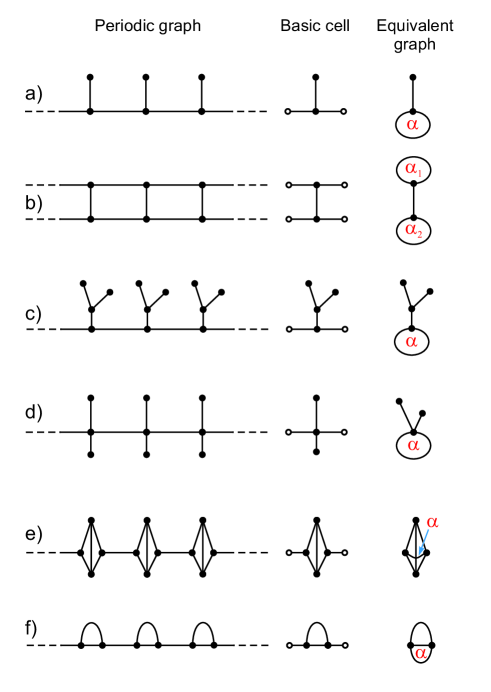
Figure 1: Some types of periodic graphs with their basic cells and corresponding equivalent graphs.

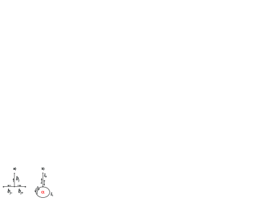
Figure 2: (a) Mapping of the $j$th basic cell of the comb graph on to its equivalent, (b) a loop vested with a magnetic flux . Arrows show directions of the assigned coordinates.

III Dirac particles on periodic quantum graphs

Here, using an extension of the approach, developed in Grisha1 , we consider a Dirac equation on a periodic graph by computing band spectra of different topologies. Within such an approach, one can treat a wide variety of periodic graphs. Although one can construct different types of periodic graphs using simple graphs as “unit cells,” we will focus on the types presented in Fig. 1. In our approach, a periodic graph is considered as a repeating structure of basic graphs, which can be called unit cells, i.e. the “graph lattice” is a periodic or quasiperiodic structure of basic graphs. We assume that in all cases, a periodic or quasi-periodic graph can be “mapped” onto the simple graphs, which (for each graph) are shown in the last column in Fig. 1. We note that there is well developed and powerful approach for the treatment of spatially periodic quantum systems, which is known under different names, such as the Bloch method, the Floquet method, and the Gelfand transformation. Within such an approach, the prescription for solving the Dirac equation on periodic graph can be formulated as follows:

1. Write Dirac equation on each bond of the basic cell;

2. Impose the vertex boundary conditions for each node of the basic cell;

3. Impose the “intercell” boundary conditions for the whole periodic graph;

4. Derive the secular equation in terms of the scattering matrix from the vertex and intercell boundary conditions;

5. Construct the scattering matrix and find eigenvalues from the secular equation.

Below we demonstrate the application of this prescription for the periodic comb graph presented in Fig. 1(a). We define the bonds of the graph as $b_{j\pm}\sim(0,l_{1}/2),\,b_{j}\sim(0,l_{2}),\,j=...,-1,0,1,...$ (see, Fig. 2). Directions of assigned coordinates on each bond are shown by arrows in Fig. 2(a). To each bond $b_{j}$ of the graph we assign a coordinate $x_{j}$, which indicates the position along the bond: for bond $b_{1}$ it is $x_{j}\in[0,l_{1}/2]$. One can use the shorthand notation $\Psi_{j}(x)$ for $\Psi_{j}(x_{j})$ and it is understood that $x$ is the coordinate on the bond $j$ to which the component $\Psi_{j}$ refers.

On each bond of this graph we have the following one-dimensional Dirac equation (in the units $\hbar=m=c=1$):

$$\begin{split}-\partial_{x}\chi_{b}+\phi_{b}&=E\phi_{b},\\ \partial_{x}\phi_{b}-\chi_{b}&=E\chi_{b},\end{split}$$ (9)

for $b\in\{b_{j-},b_{j+},b_{j}\}$.

The vertex boundary conditions for each basic cell are imposed as

$$\phi_{b_{j-}}(0) =\phi_{b_{j+}}(0)=\phi_{b_{j}}(0),$$ (10)

$$\chi_{b_{j-}}(0) +\chi_{b_{j+}}(0)+\chi_{b_{j}}(0)=0,$$ (11)

$$\chi_{b_{j}}(l_{2}) =0.$$ (12)

For the periodic graph presented in Fig. 1(a), one can impose the following quasiperiodic (inter-cell) conditions:

$$\phi_{b_{j+}}(l_{1}/2) =e^{i\alpha}\phi_{b_{j-}}(l_{1}/2),$$ (13)

$$\chi_{b_{j+}}(l_{1}/2) =-e^{i\alpha}\chi_{b_{j-}}(l_{1}/2).$$ (14)

Vertices with these boundary conditions are denoted by the empty circles in Figs. 1 and 2. It can be shown that the boundary conditions (13) and (14) do not break the self-adjointness of the Dirac operator on graph, since they are consistent with Eq.(4)

A general solution of the system of Eq. (9) can be written as

$$\left(\begin{array}[]{cc}\phi_{b}(x)\\ \chi_{b}(x)\end{array}\right)=\mu_{b}\left(\begin{array}[]{cc}1\\ i\gamma\end{array}\right)e^{ikx}+\hat{\mu}_{b}\left(\begin{array}[]{cc}1\\ -i\gamma\end{array}\right)e^{-ikx}.$$ (15)

For the whole periodic graph in Fig. 1(a), for the direction 1 [see Fig. 2(b)] the general solution can be written in terms of the following outgoing and incoming waves at the vertex:

$$\begin{split}\left(\begin{array}[]{cc}\phi_{1}(l_{1}-x)\\ \chi_{1}(l_{1}-x)\end{array}\right)&=e^{i\alpha}\left(\begin{array}[]{cc}\phi_{b_{j-}}(x)\\ -\chi_{b_{j-}}(x)\end{array}\right),\\ \left(\begin{array}[]{cc}\phi_{1}(x)\\ \chi_{1}(x)\end{array}\right)&=\left(\begin{array}[]{cc}\phi_{b_{j+}}(x)\\ \chi_{b_{j+}}(x)\end{array}\right).\end{split}$$ (16)

From the periodic boundary conditions given by Eqs.(13)-(14) and Eq.(15) we have

$$\left(\begin{array}[]{cc}\phi_{1}(y)\\ \chi_{1}(y)\end{array}\right) =\mu_{1}^{(1)}e^{i\alpha+ikl_{1}}\left(\begin{array}[]{cc}1\\ -i\gamma\end{array}\right)e^{-iky}$$ (21)

$$+\hat{\mu}_{1}^{(1)}e^{i\alpha-ikl_{1}}\left(\begin{array}[]{cc}1\\ i\gamma\end{array}\right)e^{iky},\frac{l_{1}}{2}\leq y\leq l_{1},$$ (24)

$$\left(\begin{array}[]{cc}\phi_{1}(y)\\ \chi_{1}(y)\end{array}\right) =\mu_{1}^{(2)}\left(\begin{array}[]{cc}1\\ i\gamma\end{array}\right)e^{iky}+\hat{\mu}_{1}^{(2)}\left(\begin{array}[]{cc}1\\ -i\gamma\end{array}\right)e^{-iky},$$ (31)

$$0\leq y\leq\frac{l_{1}}{2},$$ (32)

where

$$\hat{\mu}_{1}^{(1)}=\mu_{1}^{(2)}e^{-i\alpha+ikl_{1}},\,\hat{\mu}_{1}^{(2)}=\mu_{1}^{(1)}e^{i\alpha+ikl_{1}}.$$ (33)

For the direction 4 we have

$$\left(\begin{array}[]{cc}\phi_{4}(x)\\ \chi_{4}(x)\end{array}\right) =\mu_{4}\left(\begin{array}[]{cc}1\\ i\gamma\end{array}\right)e^{ikx}+\hat{\mu}_{4}\left(\begin{array}[]{cc}1\\ -i\gamma\end{array}\right)e^{-ikx}.$$ (40)

From the boundary conditions (10)-(12) we have

$$\begin{split}\mu_{1}^{(1)}&+\hat{\mu}_{1}^{(1)}=\mu_{1}^{(2)}+\hat{\mu}_{1}^{(2)}=\mu_{4}+\hat{\mu}_{4},\\ \mu_{1}^{(1)}&-\hat{\mu}_{1}^{(1)}+\mu_{1}^{(2)}-\hat{\mu}_{1}^{(2)}+\mu_{4}-\hat{\mu}_{4}=0,\\ \mu_{4}&e^{ikl_{2}}=\hat{\mu}_{4}e^{-ikl_{2}}.\end{split}$$ (41)

From Eqs.(33) and (41) we obtain the following secular equation for finding the eigenvalues of the relativistic spin-half quasiparticle on periodic quantum graph:

$$F(k;\alpha):=\det(\mathbf{I}-\mathbf{S})=0,$$ (42)

where $\mathbf{I}$ is the four dimensional identity matrix and $\mathbf{S}$ is the scattering matrix, which depends on the graph topology. For the comb graph in Fig. 1(a), the explicit form of $\mathbf{S}$ can be written as

$$\mathbf{S}=\left(\begin{array}[]{cccc}e^{-i\alpha+ikl_{1}}&0&e^{-i\alpha}-e^{ikl_{1}}&0\\ -1+e^{-i\alpha+ikl_{1}}&0&e^{ikl_{1}}-e^{-i\alpha}&e^{ikl_{2}}\\ -e^{ikl_{1}}&e^{i\alpha}&0&e^{i\alpha+ikl_{2}}\\ 0&e^{ikl_{2}}&0&0\end{array}\right).$$

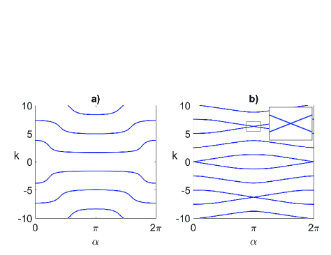
Figure 3: Band spectra of a Dirac particle on the periodic comb graph (presented in Fig. 2). Lengths are fixed by the relation $l_{1}=\beta l_{2}$, where $l_{2}$ is unit length ($l_{2}=1$) for the values $\beta=0.2$ (a) and $\beta=2.5$ (b).

IV Band spectra of the Dirac particles on periodic quantum graphs

An important characteristic of the periodic quantum structure is its band spectrum, which is the eigenenergy spectrum as a function of a system parameter. It characterizes most of the electronic properties, including electric conductance. Usually, for spatially periodic systems the band structure is symmetric with respect to the gap lying between the conductance and valence bands. This concerns also periodic branched structures described in terms of periodic quantum graphs. The periodicity of the graph is considered here with respect to basic cells. From the practical viewpoint, it is important to study dependence of the band spectra on the topology of a periodic graph and from different metric parameters of the basic cell. The latter implies the question how does the band spectrum change by changing the length of bonds connecting basic cells ($l_{1}$ in Fig. 2)?

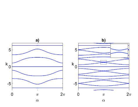
Figure 4: Band spectra of a Dirac particle on the periodic ladder graph. Lengths are fixed by the relation $l_{1}=\beta l_{2}$, where $l_{2}$ is unit length ($l_{2}=1$) for the values $\beta=0.2$ (a) and $\beta=2.5$ (b).

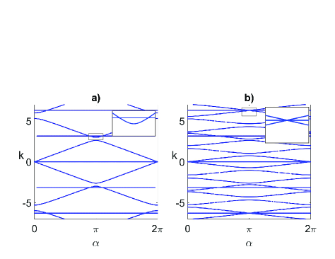
Figure 5: Band spectra of a Dirac particle on the periodic loop graph. Lengths are fixed by the relation $l_{1}=\beta l_{2}$, where $l_{2}$ is unit length ($l_{2}=1$) for the values $\beta=0.2$ (a) and $\beta=2.5$ (b).

Thus, using the secular equation (42) that holds true for an arbitrary periodic quantum graph, we calculate the band spectrum of a Dirac particle on the comb graph. We study the behavior of the band spectrum by fixing the length of $l_{2}$ as a unit and changing the length of $l_{1}$ given via the relation $l_{1}=\beta l_{2}$.

Figure 3 presents the band spectra of the comb graph [see Fig. 1(a)] plotted for two values of $\beta$: $\beta=0.2$ and $\beta=2.5$. One can observe that the gap between the levels decreases when $\beta$ increases, which means increasing the distance between ridges. Moreover, one can see level crossing (see, insets).

Similarly, one can calculate the band spectra for periodic ladder and loop graphs, presented in Figs. 1(b) and 1(f), respectively. For the sake of simplicity, for the ladder graph we choose $\alpha_{1}=\alpha_{2}=\alpha$, and for the loop graph we choose the equal lengths of the loop and the bond connecting the loop ends. The scattering matrices for these graphs can be written as

$$\mathbf{S}_{\text{ladder}}=\left(\begin{array}[]{cccccc}e^{-i\alpha+ikl_{1}}&0&0&e^{-i\alpha}-e^{ikl_{1}}&0&0\\ 0&e^{-i\alpha+ikl_{1}}&0&0&e^{-i\alpha}-e^{ikl_{1}}&0\\ 1&0&0&e^{ikl_{1}}&0&-e^{ikl_{2}}\\ -e^{i\alpha}+e^{ikl_{1}}&0&e^{i\alpha}&e^{i\alpha+ikl_{1}}&0&e^{i\alpha+ikl_{2}}\\ 0&-e^{i\alpha}+e^{ikl_{1}}&e^{i\alpha+ikl_{2}}&0&e^{i\alpha+ikl_{1}}&-e^{i\alpha}\\ 0&1&-e^{ikl_{2}}&0&e^{ikl_{1}}&0\end{array}\right),$$

$$\mathbf{S}_{\text{loop}}=\left(\begin{array}[]{cccccc}0&1&0&-e^{ikl_{1}}&e^{ikl_{2}}&0\\ 0&0&e^{-i\alpha+ikl_{3}}&0&-e^{ikl_{2}}&e^{-i\alpha}\\ e^{ikl_{1}}&0&0&1&0&-e^{ikl_{3}}\\ -e^{ikl_{1}}&e^{ikl_{2}}&0&0&1&0\\ e^{-ikl_{2}}&e^{-ikl_{2}}&-e^{-i\alpha+ikl_{3}-ikl_{2}}&-e^{ikl_{1}-ikl_{2}}&0&e^{-i\alpha-ikl_{2}}\\ -e^{ikl_{1}-ikl_{3}}&-e^{ikl_{2}-ikl_{3}}&e^{-ikl_{3}}&e^{-ikl_{3}}&e^{-ikl_{3}}&0\end{array}\right),$$

where $l_{2}=l_{3}$ according to our assumption above.

Figure 4 presents band spectra for the periodic ladder graph for the same values of $\beta$ and $l_{2}$ (the length of ladder steps). The spectral picture is the same as that for the comb graph, the gap between the levels decreases when $\beta$ increases. But the band spectrum manifests avoided crossing of the levels (see inset).

In Fig. 5 plots of the band spectra for periodic loop graph are presented for the same values of parameters as those for the comb and ladder graphs. For both values of $\beta$ a crossing of levels can be observed.

This study shows that the electronic properties of the periodic quantum structure strongly depend on the system parameter $\beta$, which in our case is the distance between basic cells.

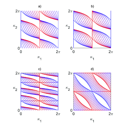
Figure 6: (color online) The zero sets of $\Phi(k_{1},k_{2};\alpha)$ for a range of values of $\alpha\in[0,\pi]$ for (a) the periodic comb, (b) ladder, (c) periodic graph shown in Fig. 2(c) and (d) loop graphs using color scale from blue ($\alpha=0$) to red ($\alpha=\pi$).

V Probability to be in the spectrum

A remarkable result of the Ref. Grisha1 , where a nonrelativistic counterpart of our problem is considered, is revealing the universal behavior of the probability that a randomly chosen momentum belongs to the spectrum of the periodic graph. Namely, the probability to be in the spectrum does not depend on the edge lengths and is also invariant within some classes of graph topologies. The basic cell classes, which manifest such a behavior are the decorations that attach to the base line by means of a single edge, e.g. as in Figs. 2(a)-2(c). Such behavior cannot be observed, for instance, in cases of decorations presented in Figs. 2(d)-2(f). Investigating such a probability and existence of universality properties for a relativistic case should be interesting both from fundamental as well as practical viewpoints.

The same trick used in Grisha1 (but originally belonging to Barra and Gaspard Barra ) can be directly applied to our case. To calculate the band spectrum of the considered periodic quantum graph: we introduce a new function

$$\Phi(\kappa_{1}=kl_{1},\kappa_{2}=kl_{2};\alpha):=F(k;\alpha),$$ (43)

where $\kappa_{1}$ and $\kappa_{2}$ need only be known modulo $2\pi$. In this way, for a fixed $\alpha$ we found solutions of

$$\Phi(\vec{\kappa};\alpha)=0,$$ (44)

where $\vec{\kappa}(k)=k\cdot(l_{1},l_{2})\mod 2\pi$ and $k$ belongs to the spectrum of the periodic graph.

Figure 6 presents dependence of $k_{2}$ on $k_{1}$ at different values of $\alpha$ calculated using Eq. (44) for the four periodic graph topologies depicted in Figs. 2(a)-2(c) and 2f.

Using the same approach used in Grisha1 , we calculate the probability $p_{\sigma}$ for a random $k$ to be in the spectrum $\sigma$. However, unlike the nonrelativistic counterpart where probability can be estimated analytically Grisha1 , in the relativistic case the secular equation has very complicated form. Therefore one should compute the probability numerically. Using the symmetry properties of the spectrum plotted in Fig. 6 one can calculate the probability by finding the area of $1/8$-th of the zero sets, which is the part in the lower left corner, bounded by the coordinate axes and the function $\kappa_{2}=\varphi(\kappa_{1};\pi)$. The numerical calculations of the probability to be in the spectrum show that for (a) comb and (b) ladder graphs and (c) the graph shown in Fig. 2(c) it takes the (same) value $p_{\sigma}\approx 0.64$, while for (d) the loop graph the probability is different, $p_{\sigma}\approx 0.73$. A similar situation was observed for the nonrelativistic counterpart considered in Grisha1 . Thus, for the relativistic case described by the Dirac equation on periodic graphs we observed similar universality for the decorations that attach to the base line by means of a single edge (at least for the topologies presented in Fig. 2).

VI Conclusions

We studied the Dirac equation on periodic quantum graphs with a focus on the eigenvalue problem. The secular equation allowing us to find a band spectrum of Dirac quasiparticles in networks is derived from quasiperiodic boundary conditions. It is shown that these latter do not break the self-adjointness of the Dirac operator on graphs. Band spectra of different periodic graphs are computed. Universality of the probability to be in the spectrum for certain graph topologies is shown by numerical calculations. The above model can find applications in the study of electronic properties of different quasi-one-dimensional branched (periodic) structures, such as, e.g., periodically branched conducting polymers, where transport of polarons can be described in terms of the Dirac equation on graphs.

References

- (1) L. Pauling, J. Chem. Phys. 4 673 (1936).
- (2) K. Ruedenberg and C.W. Scherr, J. Chem. Phys. 21 1565 (1953).
- (3) S. Alexander, Phys. Rev. B 27 1541 (1985).
- (4) P.Exner, P.Seba, P.Stovicek, J. Phys. A: Math. Gen. 21 4009 (1988).
- (5) V.Kostrykin and R.Schrader J. Phys. A: Math. Gen. 32 595 (1999)
- (6) T.Kottos and U.Smilansky, Ann.Phys., 76 274 (1999).
- (7) P.Kuchment, Waves in Random Media, 14 S107 (2004).
- (8) S.Gnutzmann and U.Smilansky, Adv.Phys. 55 527 (2006).
- (9) N.Goldman and P.Gaspard, Phys. Rev. B 77, 024302 (2008).
- (10) P.Exner and H.Kovarik, Quantum waveguides. (Springer, 2015).
- (11) G.Berkolaiko, P.Kuchment, Introduction to Quantum Graphs, Mathematical Surveys and Monographs AMS (2013).
- (12) F. Barra and P. Gaspard, J. Statist. Phys.101, 283 (2000).
- (13) S.Gnutzmann, J.P.Keating, F. Piotet, Ann.Phys., 325 2595 (2010).
- (14) D.Mugnolo. Semigroup Methods for Evolution Equations on Networks. Springer-Verlag, Berlin, (2014).
- (15) S.Gnutzmann, H.Schanz and U.Smilansky, Phys. Rev. Lett., 110 094101 (2013).
- (16) J.Bolte, G.Garforth, J. Phys. A: Math. Theor. it 50 105101 (2017).
- (17) O. Hul et al, Phys. Rev. E 69, 056205 (2004).
- (18) J.R. Yusupov, K.K. Sabirov, M. Ehrhardt and D.U. Matrasulov, Phys. Lett. A, 383, 2382 (2019).
- (19) D.U. Matrasulov, J.R. Yusupov and K.K. Sabirov, J. Phys. A, 52, 155302 (2019).
- (20) W. Bulla and T. Trenkler, Journal of Mathematical Physics 31, 1157 (1990).
- (21) J.Bolte and J.Harrison, J. Phys. A: Math. Gen. 36 L433 (2003).
- (22) J.Harrison, T.Weyand, and K.Kirsten, J. Math. Phys. 57 102301 (2016).
- (23) J.R. Yusupov, K.K. Sabirov, Q.U. Asadov, M. Ehrhardt and D.U. Matrasulov,Phys. Rev. E, 101(6) 062208 (2020).
- (24) K.K.Sabirov, J.Yusupov, D. Jumanazarov, D. Matrasulov, Phys.Lett. A, 382, 2856 (2018).
- (25) W.P. Su, Schrieffer, A.J. Heeger, Phys. Rev. Lett., 42 1698 (1979).
- (26) A.J. Heeger, Rev. Mod.Phys. 73 681 (2001).
- (27) A.J. Heeger, S. Kivelson, J.R. Schrieffer, W.-P. Su, Rev. Mod.Phys. 60 781 (1988).
- (28) D. K. Campbell and A. R. Bishop, Phys. Rev. B, 24, 8 (1981).
- (29) D. K. Campbell and A. R. Bishop, Nuclear Physics B, 200, 297 (1982).
- (30) K.K. Sabirov, J.R. Yusupov, Kh.Sh. Matyokubov, NANOSYSTEMS: Phys., Chem., Math. 11, 183 (2020).
- (31) M. Goll, A. Ruff, E. Muks, F. Goerigk, B. Omiecienski, I. Ruff, R. C. Gonzalez-Cano, J. T. L. Navarrete, M. C. R. Delgado and S. Ludwigs, Beilstein J. Org. Chem., 11, 335 (2015).
- (32) H Higginbotham, K. Karon, P. Ledwon and P. Data, Display and Imaging, 2, 207 (2017).
- (33) T. Soganci, O. Gumusay, H. C. Soyleyici , M. Ak, Polymer 134, 187 (2018)
- (34) H. Li, M.J. Catanzaro, S. Tretiak, V.Y. Chernyak, J. Phys. Chem. Lett., 5(4), pp.641-647 (2014).
- (35) F. Dreisow, M. Heinrich, R. Keil, et.al, Phys. Rev. Lett., 105, , 143902 (2010).
- (36) J. M. Zeuner, N. K. Efremidis, R. Keil, et.al., Phys. Rev. Lett., 109, 023602 (2012).
- (37) R.Band, G.Berkolaiko, Phys. Rev. Lett., 111 130404 (2013).
- (38) Yu-Ch. Luo, E. O. Jatulan, Ch.-K. Law, J. Phys. A, 52 165201 (2019).
- (39) P. Exner, O. Turek, J. Phys. A: Math. Theor. 50 455201 (2017).
- (40) D. Barseghyan, A. Khrabustovskyi, J. Phys. A: Math. Theor. 48(25) 255201 (2015).
- (41) G. Berkolaiko, M. Kha, Lett. Math. Phys. 32 (2020).
- (42) E Korotyaev, N Saburova, J. Math. Anal. Appl. 420 576 (2014).
- (43) E Korotyaev, N Saburova, J. Math. Anal. Appl. 436 104 (2016).
- (44) E Korotyaev, N Saburova, J. Funct. Anal. 272 1625 (2017).
- (45) V.Barrera-Figueroa, V.S.Rabinovich, J. Phys. A: Math. Theor. 50 215207 (2017).
- (46) L. Alon, R. Band, G. Berkolaiko, Commun. Math. Phys., 362 909–948 (2018).
- (47) G. Berkolaiko, Y. Latushkin, S. Sukhtaiev, Adv. Math. 352 632 (2019).
- (48) E Korotyaev, N Saburova, Math. Annal. 377 723 (2020).
- (49) G. Berkolaiko, Y. Canzani, G. Cox, J.L. Marzuola, preprint in arXiv:2004.12931v2, (2020).
- (50) P. Exner, J. Lipovský, Phys. Lett. A, 384 (18), 126390, (2020)
- (51) Z. Sobirov, D. Babajanov, D. Matrasulov, K. Nakamura, H. Uecker, , EPL 115 50002 (2016).
- (52) R Adami, E Serra, P Tilli, Commun. Math. Phys., 352, 387 (2017).
- (53) A. Kairzhan, D.E. Pelinovsky, J. Phys. A: Math. Theor. 51, 095203 (2018).
- (54) K.Sabirov, S. Rakhmanov, D. Matrasulov and H. Susanto, Phys.Lett. A, 382, 1092 (2018).
- (55) D. Babajanov, H. Matyoqubov and D. Matrasulov, J. Chem. Phys., 149, 164908 (2018).
- (56) J.R. Yusupov, Kh.Sh. Matyokubov, K.K. Sabirov and D.U. Matrasulov, Chem. Phys., 537, 110861 (2020).
- (57) D. Matrasulov, K. Sabirov, D. Babajanov, H. Susanto, EPL, 130 67002 (2020).