Accelerating Coupled Cluster Calculations with Nonlinear Dynamics and Shallow Machine Learning

Abstract

The dynamics associated with the time series of the iteration scheme of coupled cluster theory has been analysed. The phase space analysis indicates the presence of a few significant cluster amplitudes, mostly involving valence excitations, which dictate the dynamics, while all other amplitudes are enslaved. Starting with a few initial iterations to establish the inter-relationship among the cluster amplitudes, a supervised Machine Learning scheme with polynomial Kernel Ridge Regression model has been employed to express each of the enslaved variables uniquely in terms of the master amplitudes. The subsequent coupled cluster iterations are restricted to a reduced dimension only to determine those significant excitations, and the enslaved variables are determined through the already established functional mapping. We will show that our scheme leads to tremendous reduction in computational time without sacrificing the accuracy.

I Introduction

Coupled Cluster (CC)C̆íz̆ek (1966, 1969); Čížek and Paldus (1971); Bartlett and Musiał (2007) has established itself as an accurate tool for computing the structure and properties of atomic and molecular systems. In the CC method, one introduces an exponential wave operator $\Omega$ which folds in the effects of excited determinants on to the reference function, often taken to be the Hartree-Fock determinant; $\Omega=e^{T}$, where $T$ is a sum of many-body hole-particle excitation operators. The unknown cluster amplitudes are determined by projecting the similarity transformed Hamiltonian $G=e^{-T}He^{T}$ against the excited determinants. The correlated ground state energy is computed by evaluating the expectation value of effective Hamiltonian with respect to the chosen reference function, $E_{corr}=\langle H_{eff}\rangle=\langle e^{-T}He^{T}\rangle$. Due to the exponential wave operator, the amplitude determining equations are nonlinear and hence, one almost universally employs the iterative scheme to find the fixed points. The amplitude $t_{\mu}$ associated with the excitation operators, $T_{\mu}$ is determined by demanding $g_{\mu}=0$. Here $g$ represents the amplitudes of the similarity transformed Hamiltonian $G$, and $\mu$ is the combined hole-particle labels associated with the excited function. Clearly, in a CC scheme with single and double excitations (CCSD), the dimension of $t$’s becomes ($n_{o}n_{v}+n_{o}^{2}n_{v}^{2}$), where $n_{o}$ and $n_{v}$ are the number of hole and particle orbitals respectively, and determining these many amplitudes requires an iterative $n_{o}^{2}n_{v}^{4}$ scaling.

In a recent paperAgarawal, Chakraborty, and Maitra (2020) by the present authors, a posteriori analysis of the time series associated with the iterative scheme of a different version of the CC theory was presented. The authors introduced an input perturbation to the amplitude determining equations to probe the nonlinearity associated with the discrete-time dynamics of the iterative scheme. It was established that such equations show interesting features of the universal chaotic dynamics characterized by a full period-doubling bifurcation cascade, and that there exist nontrivial inter-relationships among the different cluster amplitudes. As such, the macroscopic features of the dynamics is solely dictated by a few large significant cluster operators (vide infra), which span a much smaller space. These cluster amplitudes behave as the order parameters, while the remaining cluster amplitudes are enslaved under the former set. Taking insight from nonlinear dynamics and SynergeticsHaken (1989); Haken and Wunderlin (1982); Haken (1983), the authors predicted a mapping of the enslaved amplitudes in terms of those significant master amplitudes. In this work, we further extend the analysis and show that it is indeed possible to exploit the master-slave multivariate dynamics to numerically map the enslaved amplitudes as functions of those significant ones. In order to establish such a mapping, we have employed a supervised machine learning (ML) strategy, based on the Kernel Ridge Regression (KRR)Murphy (2012) model and come up with a hybrid CC-ML algorithm for solving CC theory with excellent savings of computation time.

One may also note that the ML algorithm is employed to establish the synergy and inter-relationship among the cluster operators, which are predicted by the multivariate nonlinear dynamics. The methodology is solely based on the time-series dynamics associated with the iteration process, and is specific to the individual many-body system. Hence, unlike other ML methods, particularly those based on the neural network which provides data-driven solutions to CC theory, Cheng et al. (2019); Margraf and Reuter (2018); Townsend and Vogiatzis (2019); Peyton et al. (2020); Folmsbee and Hutchison (2020); Schran, Behler, and Marx (2019); Welborn, Cheng, and Miller III (2018); Schütt et al. (2019), our scheme does not require any prior computation to train the model. Contrary to that, our method is physically motivated and its origin is grafted in the dynamics of the iteration process, which allows one to map the the dependency of the cluster operators via supervised ML.

The paper is organized as follows: In Sec II we establish, via a phase space analysis, that a few large cluster amplitudes dictate the dynamics, and that the variation of all other amplitudes is suppressed. This master-slave the relationship among the cluster operators allow us to express the dependent enslaved variables as functions of the master amplitudes and we shall outline the hybrid CC-ML iterative scheme in Sec. III. We present the essential aspects of the KRR ML model in III.1, and the following section, we show how one may construct the CC equations for selected variables with much lower scaling. We will present the efficacy of our scheme in Sec. IV, and conclude our findings in Sec V.

II Establishing Master-Slave Dynamics

In order to establish the significance of the master amplitudes in the dynamics, we analyze the phase space trajectory associated with the iteration scheme. The iteration procedure is considered as a time-discrete dynamics. To visualize the multidimensional phase space in two dimensions, one may resort to the distance matrix (DM)Eckmann, Kamphorts, and Ruelle (1987); Marwan et al. (2007, 2020), which is defined as $DM_{i,j}=||\vec{x_{i}}-\vec{x_{j}}||$. Here each iteration is embedded as a single time step and $\vec{x_{i}}$ and $\vec{x_{j}}$ are the amplitude vectors at time step $i$ and $j$ respectively. Thus the $\vec{x_{k}}=(t_{1_{k}}\oplus t_{2_{k}})^{T}$. DM represents the closeness of the trajectory at two different time steps. Figure 1A depicts the DM for $H_{2}O$ at bond length = 2.6741 Bohr, bond angle = 96.774^∘ in cc-pVTZ basis. The bias in the DM towards the lower right corner indicates that the dynamics associated with the iterative scheme is convergent towards a unique set of fixed points. Such DM, however, under large input perturbation shows repetitive or chaotic phase space trajectory, as previously established by Agarawal et al.Agarawal, Chakraborty, and Maitra (2020).

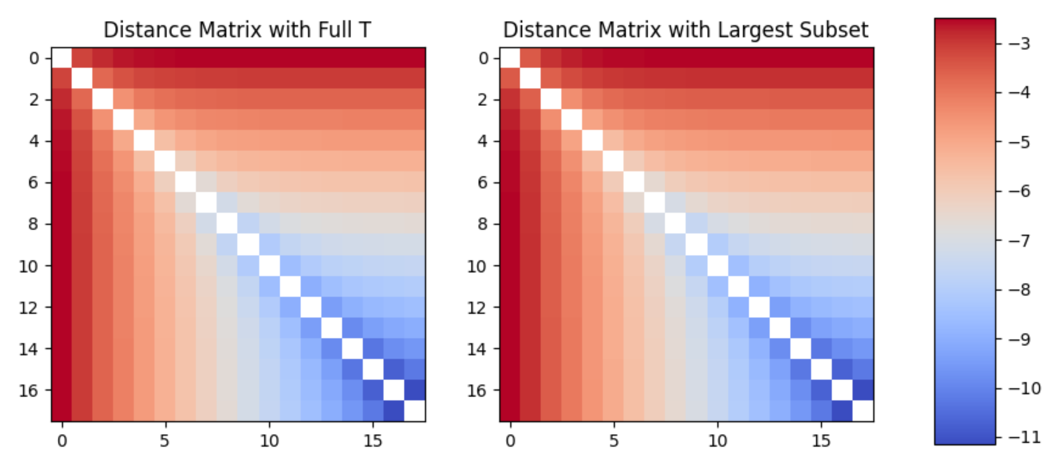
Figure 1: Distance matrix (in logarithm scale) associated with the iteration time series. The bias in the distance matrix towards the right lower corner signifies the drift towards the fixed point. Note that the diagonal will be zero, so there is no graph plotted there. Both the vertical and horizontal axes represent iteration steps.

To establish our hypothesis of a slaving dynamics, we have further constructed the amplitude vectors with only those cluster amplitudes whose magnitudes are greater than a predefined large threshold $\epsilon$. We will generically denote these amplitudes as $t^{L}$, where the superscript denotes that these set of amplitudes include only large ones and would refer to this set as the largest subset (LS). Note that the LS may include both one- and two-body excitations depending on the multi-reference nature of the molecular system under consideration. For CC theory with singles, doubles, and triples excitation scheme (CCSDT), the LS may include triple excitation as well. From a theoretical perturbation point of view, it is obvious that the excitations belonging to the LS mostly involve valence electrons. In this analysis, the choice of the threshold $\epsilon$ for selecting the LS is taken arbitrarily at 0.02 at the moment, although a more robust choice may be made through maximization of mutual information. One may note that $\{t^{L}\}$ is only a very tiny subset of the full set of cluster operators, while all other cluster amplitudes with smaller magnitudes are grouped into the smaller subset (SS), denoted by $\{t^{S}\}$. In what follows, we further construct the DM by taking into account only the LS amplitudes: $DM_{i,j}=||\vec{x^{L}_{i}}-\vec{x^{L}_{j}}||$, where $\vec{x^{L}_{k}}=(t_{1_{k}}^{L}\oplus t_{2_{k}}^{L})^{T}$ and the corresponding DM is shown in Figure 1B. It is evident from the two nearly identical DM’s that the LS qualitatively and quantitatively replicate the dynamics exhibited by the full set of cluster amplitudes. A lower choice of the threshold $\epsilon$ makes the DMs exactly identical. The choice of the molecule and the threshold discussed above is presented as a prototypical case. A similar analysis can be made for other systems as well. In other words, such an analysis is not system-specific. In a previous paperAgarawal, Chakraborty, and Maitra (2020), a similar analysis was put forward for studying the iteration dynamics under an input perturbation for regions where linear stability is lost. Thus the current work may be considered as a generalization for multivariate iteration dynamics for regions which are characterized by a unique set of fixed-point solutions.

III Synergetic Mapping of the Largest Subset to the Smaller Subset and the Feedback Coupling:

It has been established in the previous section via the full and the reduced space DMs that the macroscopic features of the iteration process is almost quantitatively governed by the LS. As such, the variation of very large number of smaller amplitudes are suppressed and thus their microscopic sub-dynamics is asymptotically negligible. The amplitudes belonging to the LS, $\{t^{L}\}$, may be considered as the order parameter of the system, which enslave the smaller ones. Let us denote the dimension of the LS by $n_{l}$. In such multivariate cases, in the regions away from fixed-point equilibrium, one may map the smaller amplitudes as unique functions of the order parameters. In other words, one may consider the elements of the LS, $\{t^{L}\}$, as independent variables of the dynamics, while those belonging to $\{t^{S}\}$ may be considered as the dependent slave variables. The dimension of the enslaved smaller amplitudes is denoted by $n_{s}$. Note that $n_{l}\textless\textless n_{s}$. For convergent regions with fixed-point equilibrium, we conjecture that for a given time step, one may write:

$$t^{S}_{\mu,k}=F_{\mu}(\{t^{L}_{k}\})$$ (1)

where $k$ represents a particular iteration step and $\mu$ is the shorthand notation of hole and particle indices associated with the excitation. Eq.1 is in principle exact for away from fixed point equilibrium regions and can be determined analytically for systems with few variables. However, it is impossible to predict this exact mapping for high dimensional cases. We have employed a supervised ML model to construct the functional form of $F_{\mu}$. In what follows, we have performed a few initial CC iterations in full dimension (space spanned by $\{t^{L}\oplus t^{S}\}$) and considered the cluster amplitudes of these initial iterations as the training data set. The polynomial regression based supervised ML model has been employed to express the small dependent amplitudes as functions of the independent order parameters. We have assumed that the exact inter-relationship among these two sets of amplitudes are established within the first few iterations and it remains unchanged over the subsequent iteration steps. Our numerical results would strongly suggest this to be a good approximation. Only the cluster amplitudes belonging to the LS, on the other hand, are determined via the conventional algebraic or diagrammatic techniques, where both sets of cluster operators couple. The coupling of the cluster operators belonging to the smaller subset (which are determined via the ML) to the equations of the amplitudes of LS may be termed as the feedback coupling. We shall show that the construction of the diagrams for the cluster amplitudes belonging to the LS can be achieved at a much cheaper scaling than the conventional way. This reduction of the independent degrees of freedom leads to the enormous savings in computational time.

In short, the overall scheme starts with $m$ conventional iterations, which are used to train the model to determine the function $F$. The accuracy of the model depends on the value of $m$. This is followed by the CC-ML hybrid iterative algorithm, which is schematically represented in Figure 2. The hybrid CC-ML algorithm involves two major steps. Step 1 performs the forward mapping of the LS amplitudes (order parameter) on to the smaller enslaved subset via Machine learning (ML), and in step 2, the enslaved variables provide the feedback coupling to determine the order parameters (LS). This is commonly referred to as the circular causality in Synergetics. In the following section, we briefly present the idea of Kernel Ridge polynomial Regression (KRR) method which maps the order parameters to the enslaved variables (step 1), and refer the readers to other ML textsMurphy (2012) for details. The next subsection will deal with the essential aspects of CC diagrammatic construction for the LS of amplitudes (step 2).

Figure 2: The circular causality loop employed in this work. The subscript quantity denotes the iteration time step. The numerous enslaved variables are determined via the functional mapping (step 1) with polynomial regression that has been established apriori via ML. The CC iterations are restricted only to determine the elements belonging to the LS (step 2).

III.0.1 Brief Account of Kernel Ridge Regression based ML Model:

As previously mentioned, the forward mapping (step 1) of the amplitudes of the LS to the smaller subset is done via polynomial Regression-based supervised ML coupled with Ridge Kernelization. This regression algorithm is based on the linear regression model, where the nonlinear terms of the independent variables are also considered as independent parameters. As we discussed, the initial few iterations were performed in the full space spanned by the entire $\{t^{L}\oplus t^{S}\}$ amplitudes and these exact amplitudes were used for training the model. As expected for any supervised machine learning algorithm, the accuracy of the model would depend on the dimension of the training data set ($N_{T}$). The linear regressor fits a set of independent variables to a set of dependent variables using the inter-dependency of the data structure. Such a generalised regression relationship can be written in a matrix form as $T^{S}=T^{L}\beta$. Here $T^{L}$ is the matrix of independent variables, which are the cluster amplitudes belonging to the LS.

$$T^{L}=\begin{pmatrix}1&t^{L}_{11}&t^{L}_{21}&...&t^{L}_{{n_{l}}1}\\ 1&t^{L}_{12}&t^{L}_{22}&...&t^{L}_{{n_{l}}2}\\ 1&t^{L}_{13}&t^{L}_{23}&...&t^{L}_{{n_{l}}3}\\ ...&...&...&...&...\\ 1&t^{L}_{1m}&t^{L}_{2m}&...&t^{L}_{{n_{l}}m}\\ \end{pmatrix}$$ (2)

Here each row signifies the independent cluster amplitudes for a fixed iteration. With $m$ number of training iterations were performed to construct the $T^{L}$ matrix, it is of the dimension $m*(n_{l}+1)$. The extra column in $T^{L}$ is added to take care of the intercept term.

Similarly, the coefficient matrix $\beta$ may be defined as:

$$\beta=\begin{pmatrix}\beta_{01}&\beta_{02}&\beta_{03}&...&\beta_{0{n_{s}}}\\ \beta_{11}&\beta_{12}&\beta_{13}&...&\beta_{1{n_{s}}}\\ \beta_{21}&\beta_{22}&\beta_{23}&...&\beta_{2{n_{s}}}\\ ...&...&...&...&...\\ \beta_{{n_{l}}1}&\beta_{{n_{l}}1}&\beta_{{n_{l}}2}&...&\beta_{{n_{l}}{n_{s}}}\\ \end{pmatrix}$$ (3)

where $n_{S}$ is the size of the dependent variable vector $T^{S}$, which is given by:

$$T^{S}=\begin{pmatrix}t^{S}_{11}&t^{S}_{21}&...&t^{S}_{n_{s}1}\\ t^{S}_{12}&t^{S}_{22}&...&t^{S}_{n_{s}2}\\ t^{S}_{13}&t^{S}_{23}&...&t^{S}_{n_{s}3}\\ ...&...&...&...\\ t^{S}_{1m}&t^{S}_{2m}&...&t^{S}_{n_{s}m}\\ \end{pmatrix}$$ (4)

Starting with a guess coefficient matrix is $\hat{\beta}$, the coefficients may be obtained by minimizing the loss function $\eta^{T}\eta$, where the error $\eta$ is given by: $\eta=T^{S}-\hat{T^{S}}$ where $\hat{T^{S}}=T^{L}\cdot\hat{\beta}$. Here $\hat{T^{S}}$ is the predicted small subset amplitudes.

Often, a linear model may not be enough to capture the features of a data set, and hence, a quadratic, cubic or some other polynomial model is used. Naturally, it leads to increase the dimension on the independent variables, and hence provide better flexibility to have a better chance of getting a good fit. One may increase the total feature vectors from $n_{l}$ to much higher dimensional space by including polynomial terms, and then each of the linear and nonlinear terms are treated as independent variables to solve using the linear regression technique. One may define a function $\phi$, which maps the given set of feature vectors to a higher dimension space by including the non linear terms:

$$\phi:\{t^{L}_{\mu},\mu\in n_{l}\}\rightarrow\{t^{L}_{\mu},t^{L}_{\mu}t^{L}_{\nu},...,(t^{L}_{\mu})^{d},\mu,\nu\in n_{l}\}$$ (5)

where $d$ is the degree of the polynomial. One may minimize the loss function with respect to $\hat{\beta}$ to arrive at an expression $\hat{\beta_{\mu}}=\phi^{T}(\phi\phi^{T})^{-1}(T^{S}_{\mu})$. However, a direct expansion to a nonlinear expressions and determination of the coefficient matrix by evaluating the above expression is computationally expensive, and hence, one often uses Kernelization technique instead, which allows evaluating the expression without explicit knowledge of the function $\phi$.

According to the Mercer theorem, one may define the Kernel Function $K=\phi\phi^{T}$ for every symmetric positive definite matrix. Thus one may write $\hat{\beta_{\mu}}=\phi^{T}(K)^{-1}(T^{S}_{\mu})$. Once the model is trained, the SS amplitudes for the $i$-th iteration are predicted using the coefficient matrix and the LS vector obtained from the same iteration.

$$t_{\mu,i}^{S}(predicted)=\phi(\{t^{L}_{i}\})\hat{\beta}_{\mu}$$ (6)

Towards this, let us define a new kernel function $K_{L}$, which takes all the previous training amplitudes and the new set of LS amplitudes of a given $i-th$ iteration to predict the new set of amplitudes $t^{S}$. Thus, $K_{L}=\phi\phi(t^{L}_{i})^{T}$, where the function $\phi$ appearing to the right is a function of the new LS amplitudes, which has been shown explicitly. Using $K_{L}$, one may obtain the predicted elements of the small component as:

$$t^{S}_{pred}=(K_{L})^{T}K^{-1}T^{S}$$ (7)

Here the subscript indicates that these are the predicted SS amplitudes.

Sometimes, the model may get unphysical underfitting or overfitting due to erroneous weight in the training data set. In order to control that, a regularization parameter is often introduced which penalizes the model each time a certain term gets unphysical weight. Thus one may modify Eq 7 by adding a regularization term to

$$t^{S}_{pred}=(K_{L})^{T}(K+\lambda I)^{-1}T^{S}$$ (8)

. Following the conventional notation used in Ridge regularization, we will denote the regularization parameter with $\alpha$. Here $\lambda=\alpha/2$. The value of $\lambda(\alpha)$ manages overfitting at the cost of rate of learning. Very small value of $\alpha$ trains the model too fast and overfits the data points, which results in slight inaccuracy with few training data sets. On the other hand, a large $\alpha$ slows down the learning process, and the model takes a larger number of training data sets to produce accurate results. Thus an optimized value of $\alpha$ is warranted for the numerical accuracy of the model.

In Eq. 8, we note that the quantity $(K+I\lambda)^{-1}T^{S}$ can be computed only once for all after the training data set is produced. Thus all the $t^{S}$ amplitudes may be computed each iteration via a single matrix multiplication of $(K_{L})^{T}$ and $(K+I\lambda)^{-1}T^{S}$, which results in huge computational time savings.

It should be noted that the method is now readily available in ML libraries and can directly be usedPedregosa et al. (2011). Therefore, while training, the inputs are a matrix of independent variables ($\{t^{L}\}$ amplitudes), and a matrix of the dependent variables ($\{t^{S}\}$ amplitudes). While predicting, the input is simply the new LS cluster amplitudes, and the output is the vector of dependent SS amplitudes.

III.0.2 Exact Determination of Order Parameters via Coupled Cluster Theory:

As previously mentioned, the LS amplitudes are determined using CC theory (step 2). Once the SS of amplitudes is generated, one may update the LS cluster amplitudes via usual Jacobi or conjugate gradient methodology.

$$t^{L}_{\mu,i+1}=t^{L}_{\mu,i}+\frac{g^{L}_{\mu,i}}{\Delta D_{\mu}}\;\;\;\;\;\;\;\;\forall\mu\in LS$$ (9)

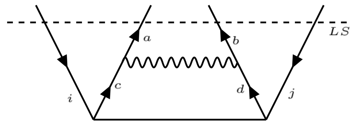
Figure 3: A representative CC linear diagram. The wiggly line denotes the two electron interaction and the solid horizontal line denotes a $T_{2}$ operator. The set of external uncontracted indices is restricted only to those sets which constitute the LS and is depicted by the dashed line, enabling a scaling reduction to $n_{l}n_{v}^{2}$ from the usual scaling of $n_{o}^{2}n_{v}^{4}$.

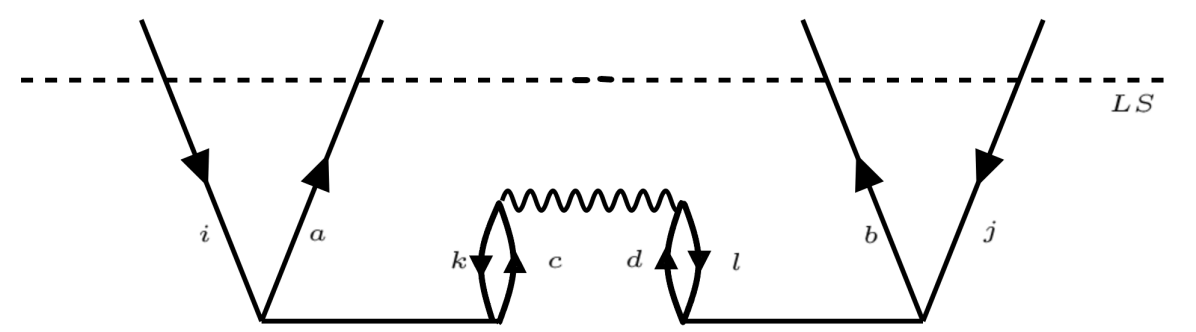
Figure 4: A representative CC nonlinear diagram. The set of uncontracted indices are restricted to only those which belong to the LS, enabling construction of the entire diagram at a scaling of $n_{l}n_{o}^{2}n_{v}^{2}$ without constructing it in a step-wise manner.

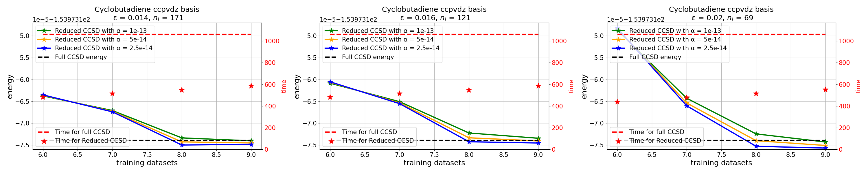
Figure 5: Predicted energies and the time taken for cyclobutadiene in cc-pVDZ basis (C-C bond = 1.88 Bohr, C-H bond = 1.313 Bohr) as functions of the training data set size (number of training iterations, $m$). The LS dimension, $n_{l}$, is explicitly mentioned for different values of $\epsilon$, and there are total 112720 nonzero cluster amplitudes. With sufficiently small $\alpha$, one gets sub $\mu E_{h}$ accuracy with 45$\%$-50$\%$ reduction in overall computation time. Note that the grid size is 5 $\mu E_{h}$. Change of $\alpha$ does not require any extra time for the calculations.

Here the orbital labels ’$\mu$’ associated with the excitations are necessarily restricted to those belonging to the LS and hence it carries the superscript $L$. The quantity $g^{L}_{\mu}$ is the residue associated with the excitation $\mu\in LS$, and $\Delta D_{\mu}$ is the usual orbital energy difference. One may note that $g^{L}_{\mu}$ can be evaluated either algebraically or diagrammatically via the Baker-Campbell-Hausdorff (BCH) multi-commutator expansions where the entire set of cluster amplitudes contribute. However, the set of external (uncontracted) indices take up only those tuples which belong to the LS. We discuss below how such a restriction simplifies the construction of CC diagrams at a cheaper computational scaling.

Let us consider the most expensive CC diagram, where two virtual orbital indices contract. In the conventional CC theory, this diagram scales as $n_{o}^{2}n_{v}^{4}$. In our modified scheme, we construct such diagrams for only those excitations where the set of uncontracted indices belong to the LS. Fig. 3 shows the diagram where the dotted line labelled $LS$, intersecting the uncontracted indices indicates the set $\{ijab\}$ necessarily belongs to the $LS$. Note that the dimension of such amplitudes is $n_{l}$. However, the cluster operators that contribute to this diagram, $t_{ijcd}$, can take any hole and particle indices. That implies $t_{ijcd}$ can belong to either the LS or SS. Thus, the total scaling to construct the diagram is simply $n_{l}n_{v}^{2}$. Note that the circular causality demands the coupling of smaller amplitudes to the equations for the LS amplitudes, and hence there is non-trivial coupling of the different amplitudes to ensure the clustering effect.

We now turn our attention to a representative nonlinear diagram. Let us consider the diagram as shown in Fig. 4. Note that in such a case, the external indices arise from two different cluster amplitudes and hence it is convenient to construct the entire diagram at once. Like the linear diagram discussed previously, the external indices are restricted to only those sets of orbitals which belong to the LS. That means the entire diagram may now be constructed at once with a scaling of $n_{l}n_{o}^{2}n_{v}^{2}$ at worst. On top of the scaling reduction, each of the nonlinear terms can be constructed at a single step, without any requirement of constructing the optimal intermediate. This further reduces the number of matrix operations by almost a factor of half. One may note that the cluster operators contributing to the nonlinear terms may belong to either the LS or the SS, and one may further judiciously approximate by including only those nonlinear terms where all the cluster operators belong to the LS. That implies that one may consider the cluster amplitudes of the SS up to the linear terms to provide the feedback coupling. We shall demonstrate in the next section that the hybrid CC-ML algorithm would enable us to compute the energetics of molecular systems with sub-microHartree ($\mu E_{h}$) accuracy with tremendous savings in computational time.

IV Results

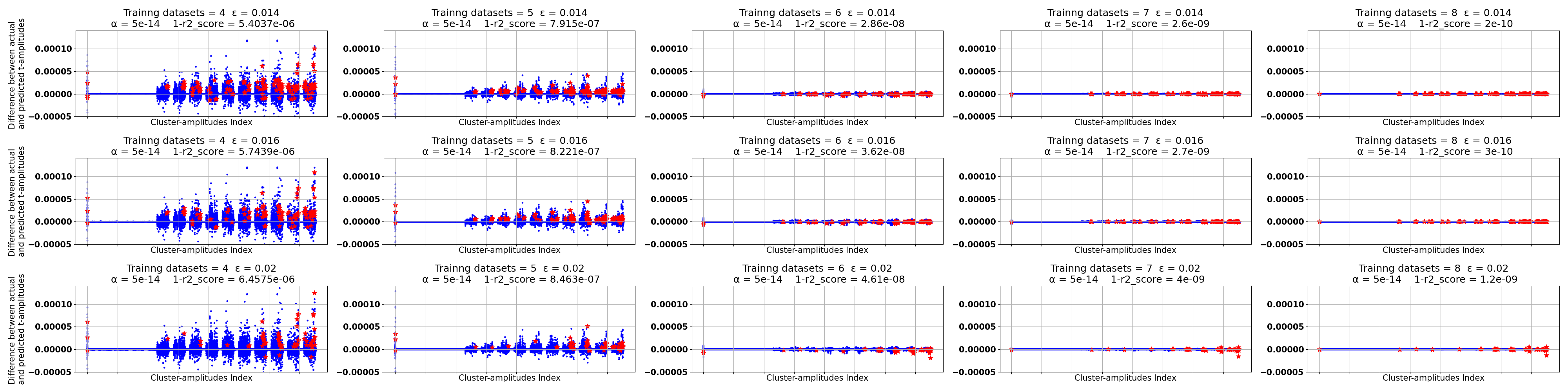
Figure 6: Difference between predicted and actual cluster amplitudes vs cluster amplitude index. Red dots denote the difference between the predicted and actual LS amplitudes, while the blue dots are for the SS amplitudes. Note the increase in accuracy of r2 score, which is represented as the difference from 1. r2 score = 1 represents perfectly accurate prediction.

In this section, we demonstrate the efficacy of our scheme with a few pilot numerical examples. We shall show that it is indeed possible to achieve very high accuracy with the hybrid CC-ML algorithm discussed previously, with a tremendous reduction in overall computation time. We first consider the case of cyclobutadiene molecule (C-C bond length = 1.88 Bohr and the C-H bond length = 1.313 Bohr), in the cc-pVDZ basis. The convergence of the predicted energy with respect to the training data set size $m$ is presented in Fig. 5 with three different threshold value $\epsilon$. Note that a lower value of the threshold $\epsilon$ signifies a larger LS dimension, $n_{l}$. Clearly, a larger LS dimension provides much more flexibility to fit the SS amplitudes as functions of those of the LS. As evident from Fig. 5, it is indeed the case as the predicted energy gets more accurate with lower $\epsilon$. The exact CCSD energy is shown with the black dashed line. Furthermore, for each value of $\epsilon$, we have plotted the predicted energy as a function of $n_{l}$ for three different regularization parameter $\alpha$. Note that for any sufficiently small $\alpha$, the predicted energy reaches sub $\mu E_{h}$ accuracy within a training data set size of eight. However, as an artifact of any regression technique, too low value of alpha leads to overfitting the model due to fast learning process, which may lead to slight inaccuracy and non-monotonic nature of energy convergence, particularly with lower training set size. On the other hand, a relatively larger $\alpha$ leads to a slow learning process, which often results in a large number of training steps to achieve similar accuracy.

We have further plotted the overall time taken by our hybrid CC-ML algorithm for different training set dimensions, and compared those against the time taken for the exact CCSD calculations with same convergence threshold and same computer architecture. The time scale is shown on the right-hand side of each plot, and the time taken by exact CCSD is denoted by the red dashed line, while the time taken by our method is shown by red dots. Note that for a given $\epsilon$ and fixed training data set dimension $m$, the time taken by our method for different $\alpha$ is almost the same and hence they are denoted by a single red dot in each plot. Clearly, with for all the threshold values $\epsilon$ reported here, our method reaches sub $\mu E_{h}$ accuracy (with training set dimension $m=8$) with almost 48$\%$ less time (with $\epsilon=0.016$, and even better time savings for larger $\epsilon$ values) compared to the time taken by the exact CCSD methods. With $m=9$, our model takes about 45$\%$ less time (with $\epsilon=0.016$) compared to the exact method for similar accuracy.

In order to gain insights into the accuracy of the predicted cluster amplitudes via the ML algorithm, in Fig 6, we have plotted the difference between our predicted cluster amplitudes and the exact converged amplitudes. Therefore, a plot with less scattered points suggests a good fit. Three different rows of the plot are for three different $\epsilon$ values, and for each $\epsilon$, we have plotted the difference in the amplitudes for different training set size with $\alpha=5\times 10^{-14}$. Clearly, for any given $\epsilon$, as we increase the training set size, the scattered points get more aligned along the $y=0$ line, signifying a high accuracy in the prediction. As evident from Fig. 2, the predicted SS amplitudes contribute to determining the LS amplitudes via the circular causality loop. Therefore, any error in prediction leads to accumulation of the error, which in turn contaminates both the LS and SS amplitudes. We note from the scatter plot that both LS amplitudes, denoted by the red dots and the SS amplitudes (denoted by the blue dots) get extremely accurate with sufficient training set size. This results in excellent accuracy in the predicted energy, as we had shown earlier. The accuracy in the prediction is also validated by computing the r2 score, which tends to one as we include more training sets into the algorithm.

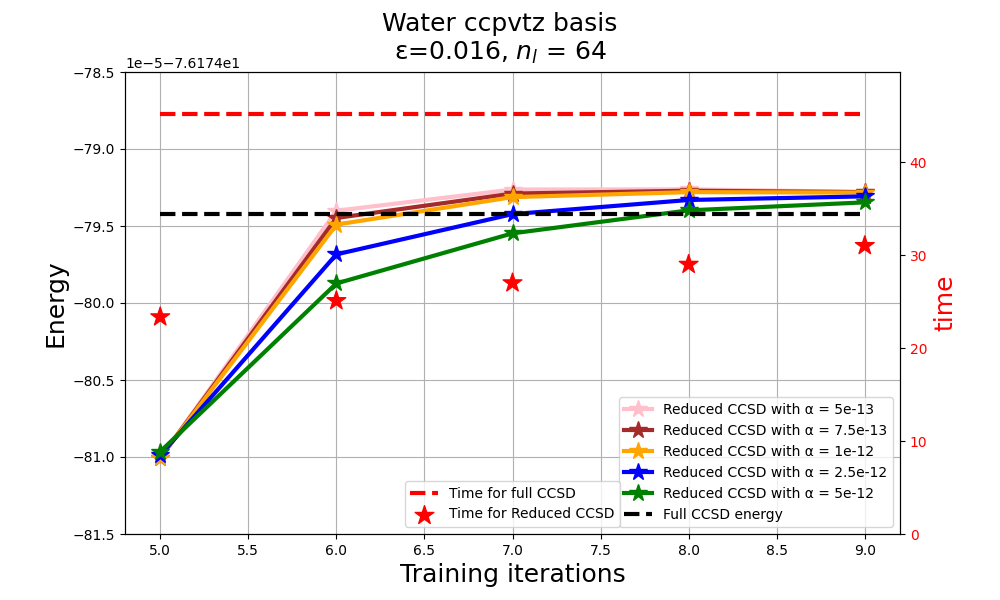
Figure 7: Predicted energies and the time taken for Water in cc-pVTZ basis (O-H bond = 2.6741 Bohr, H-O-H angle = $96.774^{\circ}$) as functions of the training data set size (number of training iterations, $m$). Note that the grid size is 5 $\mu E_{h}$.

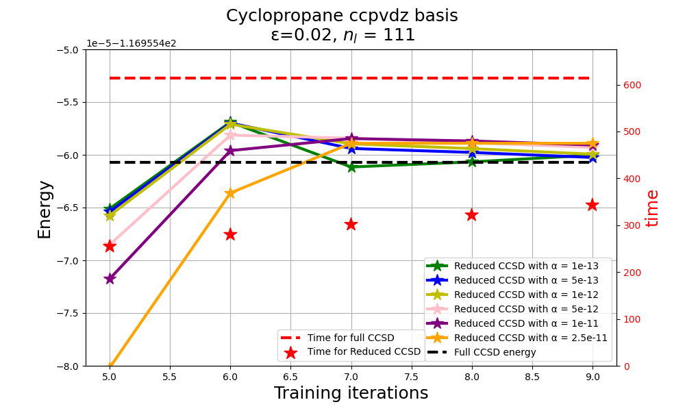
Figure 8: Predicted energies and the time taken for cyclopropane in cc-pVDZ basis (C-C bond = 2.13 Bohr, C-H bond = 1.53 Bohr, C-C-C bond angle = $60^{\circ}$, H-C-H bond angle = $114.6^{\circ}$) as functions of the training data set size (number of training iterations, $m$). Note that the grid size is 5 $\mu E_{h}$

To prove the efficacy of the algorithm across different molecules, we have also shown the accuracy of our method for water in cc-pVTZ basis (Fig. 7) and cyclopropane in cc-pVDZ basis (Fig. 8). The corresponding geometries are given along with the figures. In both the cases, one gets $\mu E_{h}$ level accuracy within 7 training set size and at 35$\%$-45$\%$ reduction in overall computation time. The slight inaccuracy and non-monotonic nature of the plot with very small $\alpha$ for cyclopropane is an artifact of overfitting due to the fast learning process. One may note that for larger molecules, further savings in computation time is expected as the LS dimension, $n_{l}$ grows sub-linearly with the system size, which makes the entire scheme a scalable one. For systems which take fewer iterations to converge, the mutual dependency among the cluster operators during the iteration process is established much earlier, which results in fewer training iteration for accurate results.

One may also note that the model involves no hidden training costs. Unlike most of the CC methods based on ML which pre-train their models on thousands of molecules to predict, our method does not require any prior training on any molecular data set, and is entirely based on the physically motivated method of multivariate dynamics and Synergetics. We argue that although the former methodologies may be faster, it hides the cost of generating the data sets via the apriori training over several molecules. Our methodology, on the other hand, has no such requirements. It is, in that sense, a standalone process, and can be executed from start to end in one go, without any prior training process.

V Conclusion

In this work, we demonstrate that the dynamics of the CC nonlinear iterative scheme is dictated by a few significant excitations, whereas thousands of cluster amplitudes are enslaved. Exploiting the basic principle of Synergetics, we employed a supervised ML scheme based on KRR model to express the enslaved dependent amplitudes in terms of the independent master amplitudes. This leads us to develop a hybrid CC-ML algorithm where only the significant master amplitudes are selectively determined via BCH multi-commutator expansion. This leads to a significant reduction in scaling for these iterations, leading to enormous savings in the overall time taken for the computation. The enslaved amplitudes, on the other hand, are predicted via the KRR model as unique functions of the master amplitudes. Our pilot numerical study demonstrates a sub $\mu E_{h}$ accuracy of the predicted energy with 40%-50% reduction in overall computation time. The method is based on physically motivated approximate schemes and does not require any apriori training on different molecules. This makes the algorithm standalone, and free of any hidden cost. Furthermore, the algorithm is based on the CC time-series dynamics, and hence it can easily be generalized to include triple, quadruple or higher excitations. Also, convergence can easily be further accelerated by using DIIS. One may further test the efficacy of other supervised or unsupervised ML schemes as there are many readily available plug-and-play ML models. This opens up the possibility of interfacing different ML models in our algorithm, which will occupy us in near future.

Data Availablity

The data to support the findings of this study are available from the corresponding author upon reasonable request.

References

- C̆íz̆ek (1966) J. C̆íz̆ek, “On the correlation problem in atomic and molecular systems. calculation of wavefunction components in ursell-type expansion using quantum-field theoretical methods,” J. Chem. Phys. 45, 4256–4266 (1966).
- C̆íz̆ek (1969) J. C̆íz̆ek, “On the use of the cluster expansion and the technique of diagrams in calculations of correlation effects in atoms and molecules,” Adv. Chem. Phys. 14, 35–89 (1969).
- Čížek and Paldus (1971) J. Čížek and J. Paldus, “Correlation problems in atomic and molecular systems iii. rederivation of the coupled-pair many-electron theory using the traditional quantum chemical methods,” Int. J. Quantum Chem. 5, 359–379 (1971).
- Bartlett and Musiał (2007) R. J. Bartlett and M. Musiał, “Coupled-cluster theory in quantum chemistry,” Reviews of Modern Physics 79, 291 (2007).
- Agarawal, Chakraborty, and Maitra (2020) V. Agarawal, A. Chakraborty, and R. Maitra, “Stability analysis of a double similarity transformed coupled cluster theory,” The Journal of Chemical Physics 153, 084113 (2020).
- Haken (1989) H. Haken, “Synergetics: an overview,” Rep. Prog. Phys. 52, 515–553 (1989).
- Haken and Wunderlin (1982) H. Haken and A. Wunderlin, “Slaving principle for stochastic differential equations with additive and multiplicative noise and for discrete noisy maps,” Z. Phys. B 47, 179–187 (1982).
- Haken (1983) H. Haken, “Nonlinear equations. the slaving principle,” in Advanced Synergetics: Instability Hierarchies of Self-Organizing Systems and Devices (Springer Berlin Heidelberg, Berlin, Heidelberg, 1983) pp. 187–221.
- Murphy (2012) K. P. Murphy, Machine learning: a probabilistic perspective (MIT press, 2012).
- Cheng et al. (2019) L. Cheng, N. B. Kovachki, M. Welborn, and T. F. Miller III, “Regression clustering for improved accuracy and training costs with molecular-orbital-based machine learning,” Journal of Chemical Theory and Computation 15, 6668–6677 (2019).
- Margraf and Reuter (2018) J. T. Margraf and K. Reuter, “Making the coupled cluster correlation energy machine-learnable,” The Journal of Physical Chemistry A 122, 6343–6348 (2018).
- Townsend and Vogiatzis (2019) J. Townsend and K. D. Vogiatzis, “Data-driven acceleration of the coupled-cluster singles and doubles iterative solver,” The journal of physical chemistry letters 10, 4129–4135 (2019).
- Peyton et al. (2020) B. G. Peyton, C. Briggs, R. D’Cunha, J. T. Margraf, and T. D. Crawford, “Machine-learning coupled cluster properties through a density tensor representation,” The Journal of Physical Chemistry A (2020).
- Folmsbee and Hutchison (2020) D. Folmsbee and G. Hutchison, “Assessing conformer energies using electronic structure and machine learning methods,” International Journal of Quantum Chemistry , e26381 (2020).
- Schran, Behler, and Marx (2019) C. Schran, J. Behler, and D. Marx, “Automated fitting of neural network potentials at coupled cluster accuracy: Protonated water clusters as testing ground,” Journal of Chemical Theory and Computation 16, 88–99 (2019).
- Welborn, Cheng, and Miller III (2018) M. Welborn, L. Cheng, and T. F. Miller III, “Transferability in machine learning for electronic structure via the molecular orbital basis,” Journal of chemical theory and computation 14, 4772–4779 (2018).
- Schütt et al. (2019) K. Schütt, M. Gastegger, A. Tkatchenko, K.-R. Müller, and R. J. Maurer, “Unifying machine learning and quantum chemistry with a deep neural network for molecular wavefunctions,” Nature communications 10, 1–10 (2019).
- Eckmann, Kamphorts, and Ruelle (1987) J.-P. Eckmann, S. Kamphorts, and D. Ruelle, “Recurrence plots of dynamical systems,” Europhys. Lett. 4, 937–977 (1987).
- Marwan et al. (2007) N. Marwan, M. C. Romano, M. Thiel, and J. Kurths, “Recurrence plots for the analysis of complex systems,” Phys. Rep. 438, 237–329 (2007).
- Marwan et al. (2020) N. Marwan, M. C. Romano, M. Thiel, and J. Kurths, “www.recurrence-plot.tk recurrence plots,” (accessed May 19, 2020).
- Pedregosa et al. (2011) F. Pedregosa, G. Varoquaux, A. Gramfort, V. Michel, B. Thirion, O. Grisel, M. Blondel, P. Prettenhofer, R. Weiss, V. Dubourg, J. Vanderplas, A. Passos, D. Cournapeau, M. Brucher, M. Perrot, and E. Duchesnay, “Scikit-learn: Machine learning in Python,” Journal of Machine Learning Research 12, 2825–2830 (2011).